The SCUBA-2 Cosmology Legacy Survey: The EGS deep field I– Deep number counts and the redshift distribution of the recovered Cosmic Infrared Background at 450 and 850​ $\mn@boldsymbol{\mu}$m

Abstract

We present deep observations at 450 $\mu\rm m$ and 850 $\mu\rm m$ in the Extended Groth Strip field taken with the SCUBA-2 camera mounted on the James Clerk Maxwell Telescope as part of the deep SCUBA-2 Cosmology Legacy Survey (S2CLS), achieving a central instrumental depth of $\sigma_{450}=1.2$​ mJy​ beam^-1 and $\sigma_{850}=0.2$​ mJy​ beam^-1. We detect 57 sources at 450​ $\mu\rm m$ and 90 at 850​ $\mu\rm m$ with S/N​ $>3.5$ over $\sim 70$ arcmin². From these detections we derive the number counts at flux densities $S_{450}>4.0$​ mJy and $S_{850}>0.9$​ mJy, which represent the deepest number counts at these wavelengths derived using directly extracted sources from only blank-field observations with a single-dish telescope. Our measurements smoothly connect the gap between previous shallower blank-field single-dish observations and deep interferometric ALMA results. We estimate the contribution of our SCUBA-2 detected galaxies to the cosmic infrared background (CIB), as well as the contribution of 24​ $\mu\rm m$-selected galaxies through a stacking technique, which add a total of $0.26\pm 0.03$ and $0.07\pm 0.01$​ MJy​ sr^-1, at 450​ $\mu\rm m$ and 850​ $\mu\rm m$, respectively. These surface brightnesses correspond to $60\pm 20$ and $50\pm 20$ per cent of the total CIB measurements, where the errors are dominated by those of the total CIB. Using the photometric redshifts of the 24​ $\mu\rm m$-selected sample and the redshift distributions of the submillimetre galaxies, we find that the redshift distribution of the recovered CIB is different at each wavelength, with a peak at $z\sim 1$ for 450​ $\mu\rm m$ and at $z\sim 2$ for 850​ $\mu\rm m$, consistent with previous observations and theoretical models.

1 Introduction

Early studies of the cosmic infrared background (CIB) showed that the Universe emits a comparable energy density at infrared (IR) and submillimetre wavelengths as it does at optical and ultraviolet wavebands, which suggests that roughly half of the star light emission is absorbed and re-emitted by dust in galaxies (e.g. Soifer et al. 1987; Puget et al. 1996; Fixsen et al. 1998). The first attempt to resolve this background resulted in the discovery of a new population of high-redshift ($z\sim 2-3$) galaxies (hereafter submillimetre galaxies, SMGs) through single-dish telescope observations at submillimetre wavelengths (e.g. Smail et al. 1997; Barger et al. 1998; Hughes et al. 1998).

The discovery of copious numbers of SMGs has proven to be a significant challenge for theoretical models of galaxy evolution. However, despite their large far-infrared (FIR) luminosities ($\ga 10^{12}$ L_⊙) and their large space density (higher than local ULIRGs), these galaxies only represent a fraction of the measured CIB (see reviews by Blain et al. 2002 and Casey et al. 2014). Previous blank field surveys resolved 20–40 per cent of the CIB at 850​ $\mu\rm{m}$ (e.g., Eales et al. 2000; Coppin et al. 2006). Meanwhile, in cluster fields 50–100 per cent of the CIB is resolved, thanks to the effect of gravitational lensing (e.g. Smail et al. 1997; Cowie et al. 2002; Knudsen et al. 2008; Chen et al. 2013), suggesting that a large fraction of this background originates from faint sources ($S_{850}<3$​ mJy) whose number counts are not yet well constrained. At shorter wavelengths, closer to the peak of the CIB ($\lambda\approx 200$​ $\mu\rm{m}$; Fixsen et al. 1998), observations with the Herschel Space Observatory have resolved $\sim 75$ per cent of the CIB at 100 and 160​ $\mu\rm{m}$ (Berta et al. 2011; Magnelli et al. 2013). Nevertheless, at 250, 350 and 500​ $\mu\rm{m}$ only a small fraction ($<25$ per cent; Oliver et al. 2010, 2012) has been resolved in individual galaxies, due to its much higher confusion limit, although, using statistical methods such as stacking and P(D), a significant larger fraction ($\approx 40-70$ per cent) can be associated with discrete sources (e.g. Glenn et al. 2010; Béthermin et al. 2012a; Viero et al. 2013b), with recent study suggesting a resolved fraction greater than 90 per cent (Viero et al. 2015; see also §5.1).

Consequently, deeper observations with higher angular resolution are still required to directly resolve and to completely understand the nature of this emission, as well as to fully determine the number counts of SMGs at fainter flux densities. These are some of the key science drivers for the SCUBA-2 Cosmology Legacy Survey (S2CLS), which exploits the capabilities of the SCUBA-2 camera (Holland et al., 2013), efficiently achieving large and deep (confusion limited) maps at both 450 and 850​ $\mu\rm{m}$, simultaneously. At the shorter wavelength, the angular resolution is $\theta_{\rm FWHM}\sim 8$​ arcsec, a factor of about 5 better than Herschel at $500$​ $\mu\rm{m}$ ($\theta_{\rm FWHM}\sim 36.6$​ arcsec), which results in a confusion limit around 7 times deeper.

On the other hand, the interferometric technique combined with the high sensitivity of ALMA has allowed the exploration of a range of flux densities unreachable through single-dish telescopes (e.g. Hatsukade et al. 2013; Ono et al. 2014; Carniani et al. 2015; Oteo et al. 2015; Aravena et al. 2016; Dunlop et al. 2016; Fujimoto et al. 2016). However, because of its relatively small field of view, it is observationally expensive to map large areas of blank sky with ALMA, and therefore difficult to constrain the less abundant population of bright galaxies. For these reasons, deep single dish telescope observations are still necessary to bridge the gap between new deep interferometric results and the past single-dish shallower studies.

Here we present 450 and 850​ $\mu\rm{m}$ observations taken in the Extended Groth Strip (EGS) field as part of the deep tier of the S2CLS (the wide tier of the survey has been presented by Geach et al. 2016). This field has been the target of the All-wavelength Extended Groth strip International Survey (AEGIS), which includes observations of some of the world’s most powerful telescopes, from X-rays to radio wavelengths. James Clerk Maxwell Telescope (JCMT) observations were scheduled to take advantage of excellent conditions ($\tau_{\rm 225GHz}<0.05$) at the top of Manua Kea, which results in the deepest single-dish telescope blank-field observations achieved at these wavelengths, comparable to the deep S2CLS maps in COSMOS and UDS (Geach et al. 2013; Roseboom et al. 2013; Koprowski et al. 2016).

In this paper we report the first results of the EGS deep study. We describe the observations and data reduction in §2. The maps and source extraction are described in §3. In §4 we report the estimated number counts at each wavelength, and in §5 the CIB fraction recovered. Finally, our results are summarized in §6. The multi-wavelength analysis, as well as a description of the physical properties of these galaxies will be presented in a subsequent paper (Zavala et al. in preparation).

All calculations assume a standard $\Lambda$ cold dark matter cosmology with $\Omega_{\Lambda}=0.68$, $\Omega_{\rm m}=0.32$, and $H_{0}=67$ kms^-1Mpc^-1 (Planck Collaboration et al. 2014).

2 Observations and data reduction

Observations at 450 and 850​ $\mu\rm{m}$ were taken, simultaneously, with the SCUBA-2 camera on the JCMT between 2012 and 2015 under the best weather conditions (band 1, $\tau_{\rm 225GHz}<0.05$) as part of the deep S2CLS in the extragalactic EGS field. A standard $\sim$5 arcmin diameter ‘DAISY’ mapping pattern (Bintley et al. 2014) was used, which keeps the pointing centre on one of the four SCUBA-2 sub-arrays during the scanning. All data were reduced using the standard SMURF package (Jenness et al. 2011; Chapin et al. 2013) with the default ‘blank field’ configuration, although the procedure for map-making (standardized across the S2CLS project) differs slightly from that described in Section 4.2 of Chapin et al. (2013). This process is described in detail in Geach et al. (2013) and Geach et al. (2016) which we summarize here, emphasizing the differences with Chapin et al. (2013).

The signal recorded by each bolometer is assumed to be a linear combination of atmospheric emission, astronomical signal (attenuated by atmospheric extinction), and a noise term. While extinction may be corrected directly using external measurements (i.e., extrapolating from $\tau_{\rm 225GHz}$ measured at the adjacent Caltech Submillimeter Observatory), the dynamic iterative map maker attempts to solve for the remaining components, refining the model until convergence is met, at which either an acceptable tolerance has been reached, or a fixed number of iterations has been completed. First, all of the bolometer data are re-sampled to a lower data rate corresponding to the Nyquist frequency for the chosen pixel size, and filtered to retain only frequencies relevant to point-sources scales, which results in a band-pass filter defined as $v/150\ {\rm arcsec}<f<v/4\ {\rm arcsec}$, where $f$ is in Hz, and $v$ is the scan speed in $\rm arcsec\ s^{-1}$. Then, each iteration consists of the following essential steps: (i) removing inter-bolometer correlated noise (primarily sky emission) via common-mode suppression (subtracting a time-varying template created from the average of all bolometer signals in a given subarray, using per-bolometer gains and offsets to fit it to the signal in question prior to removal); (ii) producing maps (on 2​ arcsec $\times$ 2​ arcsec pixel grids) from the resulting time streams which should, ideally, consist only of astronomical sources and higher-frequency (un-correlated) noise; and finally (iii) re-projecting the map back into the time-domain to estimate the contribution of astronomical sources to the bolometer signals (e.g., ‘scanning’ the detectors across the current map estimate), and then subtracting these signals, leaving primarily high-frequency, un-correlated noise from which a time-domain variance can be measured for each bolometer. The variance measured in step (iii) is used to weight the data in step (ii) in subsequent iterations. We also note that the common-mode subtraction step in (i) provides an efficient mechanism for flagging bad data: portions of bolometer signals that do not resemble the common-mode are simply masked and ignored in the remaining analysis. Since the signal-to-noise ratio (S/N) of astronomical sources is low in these fields (generally undetectable in a single bolometer signal), the solutions converge quickly. The map-maker halts when the reduced $\chi^{2}$ changes by less than 0.05, or a maximum of 20 iterations has been reached. We note that the maps are quite insensitive to the values of these convergence criteria provided that a handful of iterations are completed.

The maps produced by this procedure continue to exhibit weak large-scale noise features (though on scales smaller than the 150 arcsec cutoff in the initial band-pass filter) due to any non-white noise that may have gotten through the common-mode subtraction step. Chapin et al. (2013) advocates using jackknife maps at this stage to empirically measure this noise (i.e., dividing the data into two halves, producing maps of each, and then taking their difference to yield a map containing only noise without astronomical sources), and then constructing a ‘whitening filter’ to flatten the map to assist with source detection. While in some sense optimal, this procedure will produce a different effective PSF for each observation, making comparison between this field and others in the S2CLS more complicated. For this reason, across the S2CLS, we have opted to use a slightly more conservative (and uniform) method of large-scale noise suppression which involves subtracting a low-pass filtered map (accomplished by smoothing the map with a 30 arcsec FWHM Gaussian kernel). This method has been used by virtually all groups analyzing fields of point sources observed with SCUBA-2 data to date. In other areas of astronomy, this procedure is known as a linear unsharp mask.

Finally, in order to detect sources, we apply a matched filter to the maps, using an effective PSF constructed from an estimate of the diffraction-limited SCUBA-2 beams (Gaussians, with $\theta_{\rm FWHM}\approx 8$ and 14.5 arcsec for the 450 and 850​ $\mu\rm{m}$ bands, respectively, Dempsey et al. 2013), filtered using the same 30 arcsec FWHM background subtraction kernel (which introduces negative sidelobes). Note that this procedure is only optimal in the case that point sources are isolated in fields of uncorrelated white noise. A more sophisticated ‘confusion-compensating’ matched filter was proposed in Chapin et al. (2011) in which the effects of source blending are included explicitly in the estimate of the noise power spectrum, which in turn leads to a point-source detection kernel that behaves as the PSF described here in the low-S/N regime (when considering only instrumental noise), and smoothly converges to a de-convolution operator in the limit of infinite S/N. However, since this more optimal filter is a function of both the S/N of the observations and an estimate of the source counts in the field, it would again lead to complications when comparing different S2CLS fields. For this reason, we have opted for this simpler, uniform source-finding kernel across the project.

2.1 Astrometry

The identification of radio counterparts has been used to improve the astrometric accuracy of the submillimetre maps and to measure positional uncertainty of SMGs (e.g. Ivison et al. 2002; Chapman et al. 2005). We use the VLA/EGS 20-cm survey (Ivison et al., 2007b) for this purpose. The position of the sources in this catalogue are adopted to stack the signal in our beam-convolved SCUBA-2 maps. Figure 1 shows 30​ arcsec $\times$ 30​ arcsec postage stamps extracted from regions centred at the radio positions and stacked together. The stacked signal peaks at the central pixel in the co-added postage stamps, indicating that there is no systematic offset between the SCUBA-2 data and the radio catalogue, or it if exists, is less than our pixel size (2​ arcsec $\times$ 2​ arcsec). Therefore, no positional correction was applied.

Since the stacking could be dominated by a few bright sources, we repeated the procedure but re-normalizing each image to a constant peak brightness, finding consistent results.

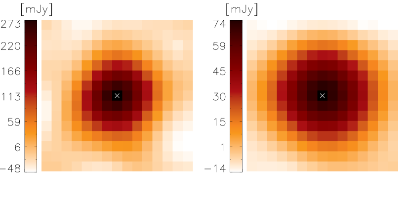
Figure 1: 30​ arcsec $\times$ 30​ arcsec co-added postage stamps of the SCUBA-2 450 and 850​ $\mu\rm{m}$ flux maps (left and right, respectively) extracted from regions centred at 39 radio source positions that lie within the SCUBA-2 map boundary (Ivison et al., 2007b). The stacked signal peaks at the central pixel for each map (white cross) which means that the astrometry of the observations is better than the 2​ arcsec pixel-size. The FHWM of the best-fit Gaussian at 450​ $\mu\rm{m}$ is 11​ arcsec $\times$ 12​ arcsec, and 14.5​ arcsec $\times$ 16​ arcsec at 850​ $\mu\rm{m}$. The $\sim$30 per cent broadening over the nominal 450​ $\mu\rm{m}$ FWHM of the PSF can be explained by a multiplicity of 20–30 per cent (as previously reported by interferometric results, e.g. Ivison et al. 2007a; Wang et al. 2011; Hodge et al. 2013) where the secondary source only contributes $\sim 20$ per cent of the total flux density.

3 Maps and source catalogue

3.1 Maps

The 450 and 850​ $\mu\rm{m}$ signal-to-noise ratio maps of EGS acquired with SCUBA-2 on the JCMT are shown in Figure 2. Each map has a radially varying coverage (see contours in Figure 2), which is roughly uniform over the central $\sim 2$ arcmin and increases radially towards the edge of the map as the effective exposure time decreases. The maximum instrumental depth achieved in the centre of each map is 1.2 and 0.2​ mJy​ beam^-1 at 450 and 850​ $\mu\rm{m}$, respectively. The noise has been estimated through a jackknife procedure where 50 per cent of the individual scans are inverted. The total area considered for source extraction is $\approx 70$ arcmin², where the r.m.s noise is below 2.5 and 0.5​ mJy​ beam^-1, respectively.

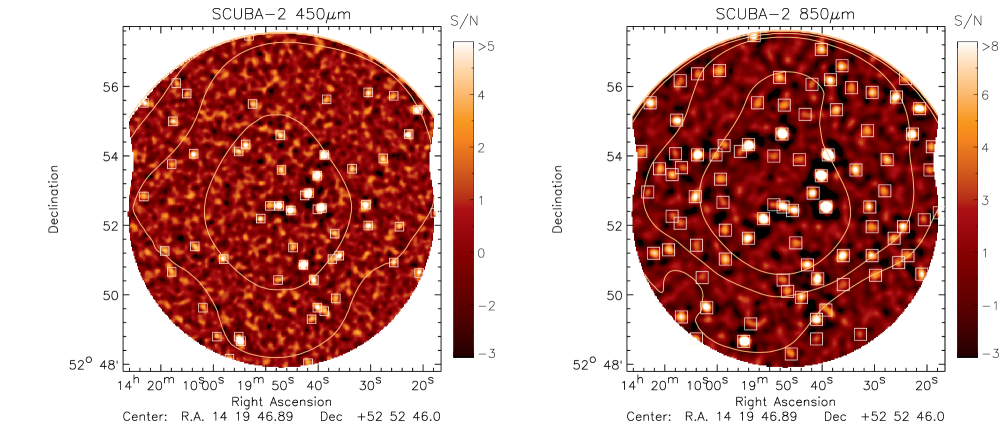
Figure 2: The 450 and 850​ $\mu\rm{m}$ Extended Groth Strip SCUBA-2 signal-to-noise ratio maps over an area of $\approx$70 arcmin². The yellow contours show the variation in the noise level, and are spaced at 0.4 and 0.05​ mJy for the 450 and 850​ $\mu\rm{m}$ maps and starting at 1.5 and 0.25​ mJy, respectively. The identified S/N$>$3.5 sources candidates are marked with yellow squares in both maps. The maps have been scaled to emphasize the visibility of the detected sources.

3.2 Source extraction and source catalogue

To identify source candidates, we search for pixels in the (beam convolved) S/N map with values $>3.0$. If a peak is found, we adopt the celestial coordinates of the pixel, the flux density and the noise, and subtract the PSF estimated in the map-making procedure scaled to the S/N measured at this position. The process is repeated until there are no more pixels with S/N​ $>3.0$. All the source candidates above this threshold are listed in Table LABEL:catalogue, together with their coordinates, measured S/N, raw flux densities, and deboosted flux densities (see §3.4). However, a conservative threshold of S/N​ $>3.5$ has been adopted to define a more robust sample. The 3.5 threshold value is chosen to be the S/N level at which the contamination rate due to false detection is estimated to be less than 5 per cent at 850​ $\mu\rm{m}$ and less than 10 per cent at 450​ $\mu\rm{m}$. At this threshold we detect 57 sources at 450 $\mu\rm m$ and 90 at 850 $\mu\rm m$. These sources are marked with squares in Figure 2.

3.3 Completeness and positional uncertainty

The detection rate for a given source within a flux density range is affected by both confusion noise from the underlying population of faint sources and instrumental Gaussian noise in the map. To account for these effects, we estimate the completeness of source detection using simulations in which mock sources with different flux densities are inserted into the observed EGS/SCUBA-2 signal maps, and then recovered with the same source extraction procedure used for the real catalogue. As described in detail by Scott et al. (2008, 2010), this method has the benefit of taking into account the effects of random and confusion noise in the signal map and, since the sources are inserted one at a time, it does not modify the properties of the real map. We insert 10,000 sources in each flux density bin, ranging from 1 to 20​ mJy (in bins of 0.5​ mJy) for the 450​ $\mu\rm{m}$ map and from 0.1 to 5​ mJy (in bins of 0.1​ mJy) for the 850​ $\mu\rm{m}$ map. A source is considered recovered if it is extracted with S/N​ $>3.5$ at a radius $<1.5$ times the size of the corresponding beam of its input position. Figure 3 shows the completeness fraction as a function of flux density for this survey.

On the other hand, the relatively large beam–size combined with the low S/N of the detections results in a significant error on the position of the source candidates. We characterize the positional uncertainty as a function of S/N from the same simulations, where now we focus on the distance at which the artificial sources were extracted. The positions of the simulated sources are chosen randomly within a pixel (instead of adopting the pixel centre) in order to take into account the 2​ arcsec $\times$ 2​ arcsec pixel size. Figure 3 also shows the median positional offset between the measured output source position and its input position as a function of S/N.

3.4 Flux deboosting

When sources are detected at low S/N, their measured flux densities are systematically larger than their intrinsic flux densities if the number of sources increases while decreasing flux (e.g. Hogg & Turner 1998). In this case it becomes more likely that the numerous faint sources are boosted high than the rarer bright sources to lower fluxes. This is particularly important in surveys of SMGs since the intrinsic population is known to have a steep distribution of counts, and also because the galaxies are typically detected at low S/N.

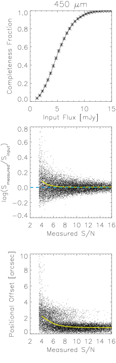
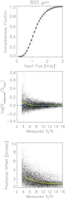
Figure 3: Top: Completeness of the 450 (left) and 850​ $\mu\rm{m}$ (right) source catalogues as a function of flux density. The points and error bars show the completeness estimated by inserting sources of known flux density one at a time into the observed signal maps and then finding them with the same source extraction algorithm used to create the source catalogue. Middle: The boosting factor estimated from the same set of simulations, measured as the ratio of output measured flux density and input flux density. The yellow solid line represents the median boosting factor in each bin of S/N and the blue dashed line represents no flux boosting. Bottom: Positional uncertainty as a function of S/N, calculated as the offset between the measured output position and its input position. The yellow line represents the median value in each bin of S/N.

In addition to the completeness and positional uncertainties, the simulations described above allow us to calculate the boosting factor. This ‘flux boosting’ is measured as the ratio of the output measured flux density and the input flux density, as shown in Figure 3. The boosting factor can also be estimated as a function of both S/N and the local noise in the map, selecting only the simulated sources that have been inserted in specific regions within a specific noise range. This selection is important, as we know that our maps have radially varying sensitivity. The error in the deboosting factor is estimated as the standard deviation in each bin of S/N and noise, and then is propagated to estimate the error in the deboosted flux density.

An alternative statistical method has been developed to correct the flux boosting. For each source candidate we can estimate a posterior flux distribution (PFD) which describes the intrinsic flux density of the source in terms of probabilities. The PFD is calculated using the Bayesian approach of Coppin et al. (2005); Coppin et al. (2006). For an individual source detected with measured flux density $S_{\rm m}\pm\sigma_{\rm m}$, the probability distribution for its intrinsic flux density $S_{\rm i}$ is given by

$$p(S_{\rm i}|S_{\rm m},\sigma_{\rm m})=\frac{p(S_{\rm i})p(S_{\rm m},\sigma_{\rm m}|S_{\rm i})}{p(S_{\rm m},\sigma_{\rm m})},$$ (1)

where $p(S_{\rm i})$ is the prior distribution of flux densities, $p(S_{\rm m},\sigma_{\rm m}|S_{\rm i})$ is the likelihood of observing the data and $p(S_{\rm m},\sigma_{\rm m})$ is a normalization factor. We assume a Gaussian noise distribution for the likelihood of observing the data, where

$$p(S_{\rm m},\sigma_{\rm m}|S_{\rm i})=\frac{1}{\sqrt{2\pi\sigma_{\rm m}^{2}}}\exp[\frac{-(S_{\rm m}-S_{\rm i})^{2}}{2\sigma_{\rm m}^{2}}]$$ (2)

This assumption is justified by the Gaussian flux distribution observed in jackknife noise maps of our EGS data (see also Geach et al. 2013).

The prior distribution of flux densities $p(S_{\rm i})$ is estimated by generating 10000 noiseless sky realizations, where sources are inserted with a uniform spatial distribution into a blank map according to a number counts distribution. Each source is assume to be the PSF scaled by the flux density. The pixel histogram of flux values from all these realizations gives an estimate of $p(S_{\rm i})$. We assume the prior number counts to be a Schechter function with the best-fitting parameters for the SCUBA-2 450 and 850​ $\mu\rm{m}$ COSMOS number counts from Casey et al. (2013) or Geach et al. (2013). We find no significant differences between the PFDs of sources estimated when using these different priors.

The deboosted flux density for each source is assumed to be the maximum value of the PFD and its associated 68 per cent confidence interval. We have compared the deboosted flux density for each source estimated using both methods, i.e. Monte Carlo simulations and the Bayesian PFD. As we can see in Figure 4, the results of both methods are in good agreement.

Finally, from the PFD, we measure the probability that each source candidate will be deboosted to less than 0​ mJy. This value could be used to exclude candidates that exceed some probability threshold, and therefore decrease the contamination of false sources in our catalogue (see Section 4).

Figure 4: Comparison between the deboosted flux density of the source candidates detected at S/N$>3.5$ (top: 450​ $\mu\rm{m}$, bottom: 850​ $\mu\rm{m}$), estimated through Monte Carlo simulations and the Bayesian method.

4 Number counts

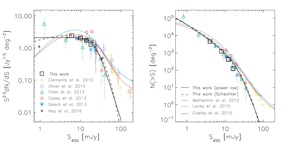
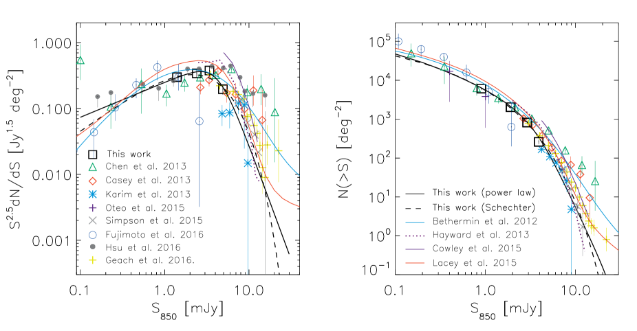
Figure 5: Left: Euclidean-normalized differential number counts of galaxies detected at 450 (top) and 850​ $\mu\rm{m}$ (bottom). Error bars indicate the 68 per cent confidence intervals. The solid black line represents the best fit using a double–power law, and the dashed black line is the best-fit using a Schechter-like function to the data described in §4. For comparison, we also plot the results from other studies and some theoretical predictions from the literature. Right: Corresponding cumulative number counts at 450 (top) and 850​ $\mu\rm{m}$ (bottom) together with integrated fits.

The cumulative number counts (also called ‘source counts’) describe the number density of galaxies as a function of flux density. To derive this quantity, we adopt the standard bootstrap sampling method that has been extensively used by different authors (e.g. Coppin et al. 2005; Coppin et al. 2006; Austermann et al. 2009, 2010). While other techniques commonly used for the extraction of number counts can in principle estimate the counts at fainter flux densities (for example the ‘P(D)’ technique; Patanchon et al. 2009; Glenn et al. 2010), it has been claimed that they are more dependent on the assumed model (see discussion in Scott et al. 2010), require constant instrumental noise across the image (which is not our case) and a good understanding of the instrumental PSF and source clustering (e.g. Vernstrom et al. 2014). On the other hand, with the Bayesian approach, the estimated counts are only weakly dependent on the assumed model of the prior distribution (Austermann et al. 2009, 2010). Since this method is described in detail in the aforementioned papers, we only briefly summarize it here.

Using the source catalogue constructed from all the source candidates with S/N​ $>3.0$ and following the procedure described in Section 3.4, we derive the PFD for each source candidate. In each realization, we randomly assign flux densities to the sources in the catalogue according to their respective PFD, and then the sources are binned to derive the differential ($dN/dS$) and cumulative [$N$($>S\rm$)] number counts, correcting each bin by the corresponding completeness and dividing by the survey area. To avoid including a large number of false positives, we only include sources whose posterior flux distribution indicates a probability of less than 5 per cent of having a negative intrinsic flux, $P$($S<0$) $\leq 0.05$. This process is repeated 500 times, also taking into account the error in completeness, in order to sufficiently sample the number count probability distribution.

We calculate the number counts at 450​ $\mu\rm{m}$ for flux densities $\geq 4$​ mJy and at 850​ $\mu\rm{m}$ for flux densities $\geq 0.9$​ mJy. At lower flux densities, the level of completeness is too low ($\leq 25$ per cent), and therefore, the errors could be large. These represent the deepest number counts derived from single-dish telescope observations towards a blank-field (i.e. without the benefit of lens amplification). It is important to remark that the confusion noise in this map has been measured to be $\sigma_{c}\approx 0.4$​ mJy​ beam^-1 at 850​ $\mu\rm{m}$, which is comparable to the instrumental noise in the map, and therefore should be taken into account. Following the results of Scott et al. (2010) we have estimated the completeness by inserting mock sources one at a time in the real flux maps (see §3.3). This method has the advantage of taking into account the confusion effects, since the sources are inserted in the real map, and does not over-predict the completeness, as when the sources are inserted into noise maps, as is commonly done in the literature.

Table 1 lists the resulting bin centres, differential and cumulative number counts, and 68 per cent confidence interval uncertainties. Figure 5 shows the cumulative and differential number counts at each wavelength.

Table 1: Differential and cumulative number counts at 450 and 850​ $\mu\rm{m}$, calculated as described in Section 4, along with the best-fit parameters.

450​ $\mu\rm{m}$-number counts					850​ $\mu\rm{m}$-number counts
S	dN/dS †	S	N ($>$S)		S	dN/dS †	S	N($>$S)
(mJy)	(mJy-1deg-2)	(mJy)	(deg-2)		(mJy)	(mJy-1deg-2)	(mJy)	(deg-2)
6.0	$873\pm 100$	4.0	$4742\pm 360$		1.4	$4076\pm 400$	0.9	$6106\pm 450$
10	$207\pm 45$​	8.0	$1250\pm 186$		2.4	$1210\pm 180$	1.9	$2030\pm 140$
14	$76\pm 20$	12	$423\pm 104$		3.4	$559\pm 100$	2.9	$820\pm 90$
18	$29\pm 16$	16	$119\pm 40$		4.9	$117\pm 20$	3.9	$261\pm 33$
Best-fit Schechter function using all data
$N_{0}$	$S_{0}$	$\alpha$			$N_{0}$	$S_{0}$	$\alpha$
$7100\pm 600$	$8.9\pm 1.5$	$2.6\pm 0.2$			$8300\pm 300$	$2.3\pm 0.5$	$2.6\pm 0.8$
Best-fit double-power law using all data
$N_{0}$	$S_{0}$	$\alpha$	$\beta$		$N_{0}$	$S_{0}$	$\alpha$	$\beta$
$600\pm 140$	$23\pm 4$	$2.5\pm 0.2$	$6.5\pm 0.2$		$1900\pm 600$	$4.3\pm 0.5$	$2.0\pm 0.4$	$6.0\pm 0.3$
Best-fit Schechter function using only S2CLS data
$N_{0}$	$S_{0}$	$\alpha$			$N_{0}$	$S_{0}$	$\alpha$
$4400\pm 2300$	$11\pm 4$	$3.1\pm 0.3$			$16000\pm 4000$	$1.3\pm 0.5$	$1.7\pm 0.8$
† The differential number counts reported in the table are not Euclidean-normalized.

We describe the differential number counts by a Schechter-like function of the form

$$\frac{dN}{dS}=\left(\frac{N_{0}}{S_{0}}\right)\left(\frac{S}{S_{0}}\right)^{1-\alpha}\exp\left(-\frac{S}{S_{0}}\right).$$ (3)

Alternatively, the number counts can also be fit with a double–power law described by

$$\frac{dN}{dS}=\frac{N_{0}}{S_{0}}\left[\left(\frac{S}{S_{0}}\right)^{\alpha}+\left(\frac{S}{S_{0}}\right)^{\beta}\right]^{-1},$$ (4)

where $N_{0}$, $S_{0}$, $\alpha$ and $\beta$ describe the normalisation, break, and slope of the power laws, respectively.

To determine the best-fit parameters we perfom a $\chi^{2}$ optimisation using a Levenberg–Marquardt algorithm. In order to better determine the best-fit parameters, we include the results from other surveys in the fitting. At 450​ $\mu\rm{m}$ we use all the SCUBA-2 measurements (Chen et al. 2013; Geach et al. 2013; Casey et al. 2013), which cover a flux density range of $S_{450}\approx 1-40$​ mJy. We exclude results from Herschel surveys at higher flux densities, since these estimates are dominated by the lensed population. At 850​ $\mu\rm{m}$ we complement our measurements at fainter flux densities with the results from SCUBA-2 observations in lensed fields (Chen et al. 2013). However, we exclude the estimates of Fujimoto et al. (2016) because of the additional uncertainty in the 1.2​ mm-to-850​ $\mu\rm{m}$ scale factor. At higher flux densities we complement our measurements with the results of ALMA observations (Karim et al. 2013; Simpson et al. 2015), and exclude the rest of the single-dish measurements, since effects of blending are more significant at these high flux densities.

The best-fit parameters for both models are listed in Table 1 and plotted in Figure  5. The errors were estimated through Monte Carlo simulations. We find that both functional forms (Schechter-like and double–power law) produce similar fits.

The last bin of our 450​ $\mu\rm{m}$ cumulative number counts lies below of our best-fit function. This is beacuse we did not find any source with $S_{450}>18$​ mJy, most likely due to cosmic variance in our relatively small map.

4.1 Comparison to other surveys

We compare our number counts at both wavelengths to the results of previously published surveys in Figure 5.

At 450​ $\mu\rm{m}$ our results are in very good agreement with the counts from the previous S2CLS map in the COSMOS field (Geach et al., 2013), which has similar depth and area. In the same field Casey et al. (2013) presented wider but shallower observations, which allowed them to estimate the number counts to brighter flux densities, and are also consistent with our values. Chen et al. (2013) and Hsu et al. (2016) combined data from cluster lensed fields and blank fields, measuring the counts over a wide flux density range. Our estimates are consistent with their results, as well as with our extrapolation of the Schechter function. At flux densities above $\sim 20$​ mJy, the number counts from our observations could be compared with the results from Herschel surveys, which mapped wider areas at 500​ $\mu\rm{m}$ to shallower depths. Our results are in agreement with the values reported by Oliver et al. (2010) and Clements et al. (2010) at $\sim 20$​ mJy, where the distributions meet. At higher flux densities the counts estimated using Herschel are dominated by rare bright and lensed galaxies that our smaller area map cannot constrain.

At 850​ $\mu\rm{m}$ the measurements from our survey are in agreement with the values of Chen et al. (2013) and Hsu et al. (2016), which came from both lensed and blank fields, except for the brighter flux density bins ($\ga 7$​ mJy), in which our extrapolation of the Schechter function lies below their estimates. The same is true for the Casey et al. (2013) results. On the other hand, at such high flux densities our extrapolation of the Schechter function is in good agreement with recently results from follow-up ALMA observations of SMGs detected with single dish telescopes (Karim et al. 2013; Simpson et al. 2015), and with the number counts derived from $\sim 5$ deg² SCUBA-2 observations (the largest and deepest single survey at 850​ $\mu\rm{m}$ so far; Geach et al. 2016). At fainter flux densities, our results overlap with the deep 870​ $\mu$m ALMA observations presented by Oteo et al. (2015) in excellent agreement, although their uncertainties are large because of the small number of sources detected (11 sources in $\sim 6$ arcmin² combining ALMA observations at different depths). At the same time, our estimations are consistent with the results at 1.2​ mm (scaled to 850​ $\mu\rm{m}$ by a factor of 2.3, assuming a typical SED at $z\sim 2$) by Fujimoto et al. (2016), which include all the archival deep data at that time (including data from other deep ALMA observations, e.g. Hatsukade et al. 2013; Ono et al. 2014; Carniani et al. 2015), compiling a sample of 133 sources within $\sim 10$ arcmin².

Excluding the results from Chen et al. (2013) and Hsu et al. (2016), which use the benefit of lensing amplification, this is the first time that single-dish blank field observations have connected with the results from deep interferometric measurements. This results in a better understanding of the number counts towards fainter flux densities.

Since we have included previously reported number counts in our fits, may not be surprising that our results are in agreement with previous estimates of the number counts. To test if our data alone are in good agreement with previous results, we again run the fitting procedure, but just using our measurements. Here we only apply the Schechter function since the double–power law has one more free parameters, making it impractical to fit to just four bins. The best-fit parameters are listed in Table 1. At 450​ $\mu\rm{m}$, although the parameters of the Schechter function are different, the fit is in very good agreement with the values in the literature, from about $1-40$​ mJy. At 850​ $\mu\rm{m}$, our measurements are in good agreement with the brighter flux density estimations, however, at fainter flux densities ($<0.5$​ mJy) our extrapolation of the Schechter function is below the measurements of Chen et al. (2013) (although still consistent within the error bars), but in very good agreement with the ALMA estimates of Oteo et al. (2015).

4.2 Comparison to models

In this section, we compare the 450 $\mu$m and 850 $\mu$m number counts presented in this work to the results of recent galaxy formation models. Lacey et al. (2015), presented a new version of the GALFORM semi-analytical model, which includes improvements to the prescription for AGN feedback, disk–instability–driven starbursts, and stellar population models. Cowley et al. (2015) implemented also the effect of the beam–size on the observed number counts on the GALFORM model to study the possible bias introduced by the source blending of individual sources. However, they conclude that the beam size at 450​ $\mu\rm{m}$ does not produce any significant enhancement of the source density. In Figure 5, it can be seen that the number counts predicted by GALFORM appear to be in broad agreement with the results presented here within the 450 $\mu$m flux density range of $S_{450}$ = 3–30 mJy. However, while the shape of the number counts are broadly similar we identify a small offset between the observed counts and the theoretical predictions, where the GALFORM source density lie a factor of $\sim 1.3$ above of our integrated measurements. In contrast, at the faintest flux the model underpredict the number of sources (a factor $\sim 2$ in the cumulative number counts at $S_{450}\approx 0.6$​ mJy). At higher flux densities, the number counts become dominated by the lensed population that, as described in the previous section, our survey has insufficient area coverage to constrain accurately. We also compare to the Béthermin et al. (2012b) model, which is based on the evolution of the main-sequence of star-forming galaxies and a second population of starburst galaxies, assuming some spectral energy distribution templates. The results of Béthermin et al. (2012b) are similar to the GALFORM model and therefore are in reasonable agreement with our measurements, albeit with a marginally larger offset of $\sim 1.7$ above our cumulative counts (Figure 5.)

At 850​ $\mu\rm{m}$ the number counts predicted by the GALFORM model (Lacey et al. 2015) also follow the behavior of our best-fit source counts at flux density of $S_{850}$ = 0.2–10 mJy. Although, we again note that the theoretical counts are systematically a factor $\sim 1.5$ above the observed values. Interferometric observations have shown that the source blending at this wavelength is more important due to the larger beam–size (e.g. Wang et al. 2011; Hodge et al. 2013). This effect is also predicted by Cowley et al. (2015) when taking into account the coarser angular resolution in the GALFORM model. The Béthermin et al. (2012b) predictions are also in agreement (but also a factor $\sim 1.4$ above our best-fit integrated functions), nevertheless, when compared with our estimates and the Geach et al. (2016) results, the model overpredicts the counts at $S_{850}\ga 8$​ mJy, for example, by a factor of $\sim 5$ in the cumulative counts at $S_{850}\approx 16$​ mJy (see Figure 5). Finally, we also compare our measurements to the model of Hayward et al. (2013) based on the bolshoi cosmological simulation, which also takes into account the blending in single-dish observations. The predictions for a 15^′′ beam are consistent with our number counts, however, this model predicts that the multiplicity caused by blending increases the number counts by more than an order of magnitude. This has been ruled out by recent interferometric results which found that the number counts are boosted by only 20 per cent at $S_{870}>7.5$​ mJy, and 60 per cent at $S_{870}>12$​ mJy (Simpson et al. 2015).

5 Contribution to the Cosmic Infrared Background

5.1 The resolved CIB

Once we have extracted the point sources with S/N​ $>3.5$ from our maps, we can estimate the contribution of these sources to the CIB at each wavelength, corrected for completeness, by integrating the number counts above our flux density limit. To do this we integrate the best-fit number counts (those derived when used all the data) at $S_{450}>4.0$​ mJy and $S_{850}>0.9$​ mJy. At these flux densities the integration of both the double-power law and the Schechter function give us the same results. The integrated intensities of our detected galaxies are $I_{\nu}(450\mu\rm{m})=(0.13\pm 0.03$​ MJy​ sr^-1 and $I_{\nu}(850\mu\rm{m})=0.04\pm 0.01$​ MJy​ sr^-1, which correspond to $28\pm 13$ and $28\pm 14$ per cent, respectively, of the CIB measured by the COBE Far-Infrared Absolute Spectrophotometer (FIRAS, Fixsen et al. 1998), where the uncertainties are dominated by those of the total CIB values. Extrapolating the number counts below our detection limits, we find that the total CIB is resolved at $S_{450}\approx 0.6$​ mJy and $S_{850}\approx 0.02$​ mJy, respectively.

There have been other measurements of the total values of the CIB based on both direct measurements, for example of COBE Difuse Infrared Background Experiment (DIRBE, Hauser et al. 1998) and COBE FIRAS (Lagache et al. 1999), and integrated galaxy-counts derived from Spitzer and Herschel (e.g. Dole et al. 2006; Berta et al. 2011; Béthermin et al. 2012a; see also recent compilation by Driver et al. 2016). However, the uncertainties remain large, and therefore, better estimates of the absolutes CIB values are still required to better constrain the fraction contributed by these galaxies. Here we adopt the values of Fixsen et al. (1998) in order to consistently compare our results to previous similar studies (e.g. Viero et al. 2015).

To measure the contribution to the CIB by galaxies fainter than our detection threshold, we stack the maps at the positions of 24​ $\mu\rm{m}$ galaxies selected from a Spitzer catalogue in the EGS field (Barro et al., 2011a, b). This technique has been implemented before by different authors (e.g. Marsden et al. 2009; Béthermin et al. 2012a; Viero et al. 2013b; and references therein), and used by Geach et al. (2013) in the COSMOS/S2CLS survey. First, we remove point sources detected with S/N$>3.5$ from the maps using a point spread function (PSF) normalized to the flux of each individual source in our catalogue. Then, we subtract the mean of the SCUBA-2 maps, which yields a residual map, where the flux corresponds to sources that are not present in our catalogues (in addition to noise). Finally, the 450 and 850​ $\mu\rm{m}$ maps are stacked at the position of the 24​ $\mu\rm{m}$ sources, averaging the flux at each position.

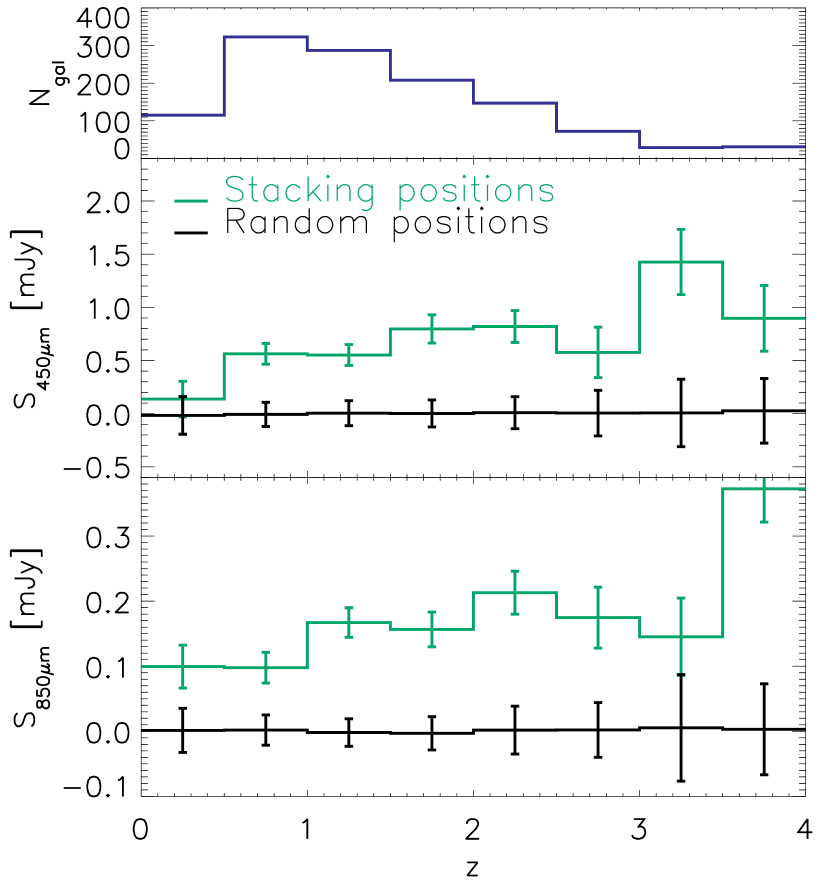
Figure 6: Stacked average flux density at 450 and 850​ $\mu\rm{m}$ (green line in the middle and bottom panels, respectively) as a function of redshift at the position of the 24​ $\mu\rm{m}$-selected galaxy sample. The top panel represents the number of galaxies in bins of redshift used in the stacking procedure. The black lines represent the results of null tests, in which the stacking was done at random positions, finding an average stacked flux of zero.

Since the 24​ $\mu\rm{m}$ source catalogue includes photometric redshifts, we can estimate the stacked flux density as a function of redshift, as shown in Figure 6. The uncertainty is estimated as $\sigma/\sqrt{N}$, with $\sigma$ is the standard deviation in the stack and $N$ the sample size (which is represented in the top panel of Figure 6). To ensure that the recovered stacked flux comes from the 24​ $\mu\rm{m}$ sample and not from noise or other contaminants, we repeat the same procedure but at random positions, conserving the number of stacked positions in each redshift bin. As shown in Figure 6, the average stacked flux from the random positions is zero, which means that the recovered fluxes are actually associated with the 24​ $\mu\rm{m}$ population.

The total intensities recovered by the stacking are $I_{\nu}(450\mu\rm{m})=0.13\pm 0.01$ MJy sr^-1 and $I_{\nu}(850\mu\rm{m})=0.03\pm 0.003$ MJy sr^-1, which corresponds to $28\pm 11$ and $21\pm 9$ per cent of the CIB, respectively, including the uncertainties in the absolute CIB values

The contribution of the directly detected sources and the stacking of 24​ $\mu\rm{m}$ galaxies amount a total $0.26\pm 0.03$ and $0.07\pm 0.01$ MJy sr^-1 at 450 and 850​ $\mu\rm{m}$, respectively, which correspond to $\sim 60\pm 20$ and $50\pm 20$ per cent of the total CIB measurements. This is in excellent agreement with the estimations by Béthermin et al. (2012a), who using the 24​ $\mu\rm{m}$ sources as priors, estimating that the emission of galaxies down to $\sim 2$​ mJy at 500​ $\mu\rm{m}$ contributed $\sim 55$ per cent of the CIB.

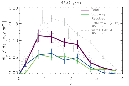
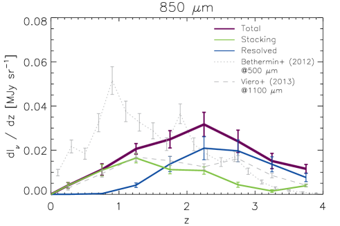
Figure 7: Redshift distributions of the recovered intensity, $dI_{\nu}/dz$, at 450​ $\mu\rm{m}$ (left) and 850​ $\mu\rm{m}$ (right). The blue line represents the contribution of the point sources directly detected in the SCUBA-2 maps and the green line represents the contribution from stacking 24​ $\mu\rm{m}$-detected galaxies. The total contribution is plotted as a purple line. For comparison we plot the results from Béthermin et al. (2012a) at 500​ $\mu\rm{m}$ and from Viero et al. (2013b) at 500 and 1100​ $\mu\rm{m}$. The 500​ $\mu\rm{m}$ values have been multiplied by a factor of 1.2 and 0.36 to scale their total intensities to match our 450 and 850​ $\mu\rm{m}$ maps, while the 1100​ $\mu\rm{m}$ are scaled by 1.75 to match our 850​ $\mu\rm{m}$ measurements, according to the absolute values measured by Fixsen et al. (1998),

An important concern in the stacking technique is the possible bias due to clustering, which can result in a boosted average flux density arising from faint, companion (or clustered) galaxies (e.g. Serjeant et al. 2008; Kurczynski & Gawiser 2010; Heinis et al. 2013). This effect increases with the size of the beam. However, using a 24​ $\mu\rm{m}$ catalogue and the Herschel maps, Béthermin et al. (2012a) found that this bias is only $5-7$ per cent at 250​ $\mu\rm{m}$, which has ${\rm FWHM}=18.1$ arcsec. Our 850​ $\mu\rm{m}$ beam has ${\rm FWHM}=14.5$ arcsec, and therefore, the expected bias due to clustering should be less than 5 per cent (and even less at 450​ $\mu\rm{m}$ with a beamsize of ${\rm FWHM}=8$ arcsec). Given the uncertainties in our measurements and the absolute values of the CIB, we have not included any clustering correction in our estimations

Considering that roughly half of the CIB is still missing at both wavelengths it is important to discuss the possible origin for this missing fraction. The first point to consider is that we do not correct our stacking measurements for the completeness of the 24​ $\mu\rm{m}$-selected catalogue. As discussed in earlier studies (e.g. Béthermin et al. 2012a), the stacking of an incomplete catalogue biases the result, missing a significant fraction of the intensity. Béthermin et al. (2013) show that an $S_{24\mu\rm m}>80$​ $\mu\rm{Jy}$ selection could miss up to half of the intensity expected from all galaxies, which could account for the remaining CIB.

Actually, Viero et al. (2015) studied the contribution of galaxies which are not detected in current near-infrared surveys, for example, very low-mass or very dusty galaxies, but which are correlated (i.e. clustered) with the detected galaxies. To account for these uncatalogued sources they intentionally smoothed and stacked Herschel observations. They found that the contribution of these galaxies is very important, especially in the $1<z<4$ range (where the completeness is low), and could fully explain the rest of CIB at 250 – 500​ $\mu\rm{m}$. However, at longer wavelengths (i.e. $\lambda\ga 850$​ $\mu\rm{m}$), deep interferometric observations (e.g Chen et al. 2014; Fujimoto et al. 2016) have shown that only $\sim 50$ per cent of the faint submillimetre galaxies ($S_{850}\la 2$​ mJy) are detected in deep optical/NIR surveys, suggesting that many of these sources, which also contribute to the CIB, are high redshift galaxies ($z\ga 3$).

5.2 The redshift distribution of the recovered CIB

As described above, the stacking analysis was performed in bins of redshifts, which allowed us to estimate the contribution of these galaxies as a function of redshift. The green line in Figure 7 represents the redshift distribution of the recovered intensity from the stacking of 24​ $\mu\rm{m}$ prior positions at 450 and 850​ $\mu\rm{m}$.

To estimate the redshift distribution of the intensity produced by the galaxies formally detected in our SCUBA-2 maps we adopt previously published redshift distributions of similar populations. For the 450​ $\mu\rm{m}$-detected galaxies we use the distribution of Roseboom et al. (2013), which comprises photometric redshifts of 450​ $\mu\rm{m}$-selected galaxies detected in deep SCUBA-2 observations ($\sigma_{450}=1.5$​ mJy), similar to the depth of our map, and therefore, galaxies with similar flux densities. This redshift distribution shows a broad peak in the range $1<z<3$, and a median of $z=1.4$ (Roseboom et al., 2013). For the 850​ $\mu\rm{m}$ galaxies we consider the redshift distribution of Chen et al. (2016), derived from a large sample of SCUBA-2-detected galaxies with $S_{850}>1$​ mJy, which has a median redshift of $2.6\pm 0.1$, in consistency with the deep ($\sigma_{850}=0.25$​ mJy) S2CLS COSMOS map (Koprowski et al. 2016) and with previous observations of brighter sources (e.g. Chapman et al. 2005). Figure 7 indicates the intensity as a function of redshift which is contributed by the galaxies detected in our maps at both wavelengths, this being the result of scaling the redshift distribution to the corresponding intensity. The redshift distribution of the total intensity (stacked plus directly detected sources) is also and is reported in Table LABEL:diff_CIB.

As shown in Figure 7 the redshift distribution of the recovered CIB is different at the two wavelengths, with sources at higher redshifts contributing more at 850​ $\mu\rm{m}$. At 450​ $\mu\rm{m}$ our results show a peak at $z\sim 1$, in very good agreement with the measurements at 500​ $\mu\rm{m}$ by Béthermin et al. (2012a), which come from 24​ $\mu\rm{m}$ catalogues, and with Viero et al. (2013b), who stacked K band–selected sources in Herschel maps. Their values have been plotted in Figure 7 (left panel) multiplied by a factor of 1.2 to scale the 500​ $\mu\rm{m}$ estiamtes to our 450​ $\mu\rm{m}$ measurements, according to the flux density ratio of the CIB spectrum (Fixsen et al. 1998). At 850​ $\mu\rm{m}$ the redshift distribution of the recovered intensity peaks at $z\sim 2$ (see right panel of Figure 7). We have again plotted the values of Béthermin et al. (2012a) (scaled to 850​ $\mu\rm{m}$ by a factor of 0.36) as a comparison. As shown in this Figure, the Béthermin et al. redshift distribution is inconsistent with our values, clearly showing that the contribution of higher redshift sources is more important at longer wavelengths. Our estimated redshift distribution is, on the other hand, similar to the one found by Viero et al. (2013b) but at 1100​ $\mu\rm{m}$. Their results (scaled at 850​ $\mu\rm{m}$ by a factor of 1.75) are also plotted in Figure 7.

Our results, highlight that the redshift distribution of the CIB depends on wavelength, with the peak shifting to higher redshifts for longer wavelength bands, and vice versa, as also measured by Marsden et al. (2009), Berta et al. (2011), Béthermin et al. (2012a), and Viero et al. (2013b). This is also consistent with the predictions of different theoretical models of the CIB (e.g. Valiante et al. 2009; Béthermin et al. 2013; Viero et al. 2013a; Mancuso et al. 2016). This selection effect has also been observed in the redshift distributions of submillimetre galaxies selected at different wavelengths, in which shorter wavelengths select lower-$z$ galaxies (and hotter sources), and can be explained with a single population of galaxies (Zavala et al. 2014, Béthermin et al. 2015)

On the other hand, Schmidt et al. (2015), using Planck data, have measured a peak at $z\sim 1.2$ for 350, 550 and 850​ $\mu\rm{m}$ observations, with no obvious wavelength dependence, however, the uncertainties around the peak are large enough to hide or mask out the possible evolution as a function of wavelength, as discussed by these authors.

As discussed above, most of the remaining CIB is expected to be emitted by obscured or low-mass galaxies at $z<4$ that are not present in the optical/NIR catalogues due to incompleteness, as suggested by the recent work of Viero et al. (2015). However, they also found tentative evidence of higher redshift ($z>4$) contributions to the CIB at 500​ $\mu\rm m$. This population of high-$z$ galaxies, which is unreachable with the current optical/NIR surveys (e.g. Kohno et al. 2016), may also contribute to the CIB (although to a lesser extent), especially at longer wavelengths. Actually, Fujimoto et al. (2016) found that the full CIB at 1.2​ mm is explained by sources with $S_{1.2}>0.02$ mJy, but only half of the faintest galaxies ($0.02<S_{1.2}<1.2$​ mJy) has an optical/NIR counterpart, and none has a radio, suggesting a high-redshift ($z>3$) nature.

Table 2: Differential recovered intensity as a function of redshift at 450 and 850​ $\mu\rm{m}$ (as plotted in Figure 7).

Redshift	450​ $\mu\rm{m}$	850​ $\mu\rm{m}$
	($\times 10^{-2}$ MJy sr-1)
$0.0<z<0.5$	$3.0^{+1.3}_{-1.1}$	$0.3^{+0.1}_{-0.1}$
$0.5<z<1.0$	$12.3^{+2.5}_{-2.0}$	$0.9^{+0.3}_{-0.3}$
$1.0<z<1.5$	$12.3^{+2.5}_{-2.0}$	$2.3^{+1.1}_{-0.6}$
$1.5<z<2.0$	$9.0^{+1.8}_{-1.5}$	$3.0^{+2.6}_{-1.3}$
$2.0<z<2.5$	$9.4^{+2.1}_{-1.6}$	$3.5^{+3.0}_{-1.4}$
$2.5<z<3.0$	$4.4^{+1.1}_{-0.9}$	$2.2^{+2.2}_{-1.1}$
$3.0<z<3.5$	$1.8^{+0.4}_{-0.4}$	$1.1^{+1.3}_{-0.6}$
$3.5<z<4.0$	$1.0^{+0.3}_{-0.3}$	$0.7^{+0.6}_{-0.3}$

6 Summary

We have presented deep SCUBA-2 observations at 450 and 850​ $\mu\rm{m}$ in the EGS field as part of the SCUBA-2 Cosmology Legacy Survey. This survey, together with other similarly deep S2CLS maps, represents one of the deepest blank-field observations achieved with single-dish telescopes, reaching a depth of $\sigma_{450}=1.2$​ mJy and $\sigma_{850}=0.2$​ mJy, respectively. Using 57 sources detected above $3.5\sigma$ at 450​ $\mu\rm{m}$ and 90 at 850​ $\mu\rm{m}$ we estimate the number counts and the contribution of these galaxies to the cosmic infrared background.

Our number counts at 450​ $\mu\rm{m}$, at a flux density limit of $S_{450}>4.0$​ mJy, are in good agreement with the previous estimation by Geach et al. (2013) derived from S2CLS observations in the COSMOS field. Our result is also consistent with previous shallower observations in blank and gravitational lensed fields.

At 850​ $\mu\rm{m}$ our results are the first number counts reported from the deep tier of the S2CLS, and therefore these represent the deepest number counts derived from single-dish blank-field observations using only directly-detected sources. Our estimations are in agreement with the number counts achieved through the benefit of gravitational lensing and with the recent results from interferometric observations with ALMA.

We have also estimated the contribution of the detected sources to the CIB and the contribution of 24​ $\mu\rm{m}$-detected galaxies throughout a stacking technique, which give a total of $0.26\pm 0.03$ and $0.07\pm 0.01$ MJy sr^-1, at 450​ $\mu\rm m$ and 850​ $\mu\rm m$, respectively, corresponding to $60\pm 20$ and $50\pm 20$ per cent of the CIB. Using the photometric redshifts available for the 24​ $\mu\rm{m}$-detected sample and previously published redshift distributions of the 450 and 850​ $\mu\rm{m}$ blank-field population, we decompose this emission into bins of redshift, finding an evolution of the redshift distribution of the recovered CIB as a function of wavelength, which peaks at $z\sim 1$ at 450​ $\mu\rm{m}$, whereas at 850​ $\mu\rm{m}$ it peaks at $z\sim 2$, in agreement with theoretical models and previous observations.

The remaining CIB is expected to be emitted by galaxies that are too faint at 24​ $\mu\rm{m}$ to have been detected in Spitzer surveys, as discussed by other authors, although a contribution of high-redshift ($z>4$) galaxies could also be important, especially at the longer wavelength.

Appendix A Source catalogues

The catalogues will be released in the published version.

References

- Aravena et al. (2016) Aravena M., et al., 2016, preprint, (arXiv:1607.06769)
- Austermann et al. (2009) Austermann J. E., et al., 2009, MNRAS, 393, 1573
- Austermann et al. (2010) Austermann J. E., et al., 2010, MNRAS, 401, 160
- Barger et al. (1998) Barger A. J., Cowie L. L., Sanders D. B., Fulton E., Taniguchi Y., Sato Y., Kawara K., Okuda H., 1998, Nature, 394, 248
- Barro et al. (2011a) Barro G., et al., 2011a, ApJS, 193, 13
- Barro et al. (2011b) Barro G., et al., 2011b, ApJS, 193, 30
- Berta et al. (2011) Berta S., et al., 2011, A&A, 532, A49
- Béthermin et al. (2012a) Béthermin M., et al., 2012a, A&A, 542, A58
- Béthermin et al. (2012b) Béthermin M., et al., 2012b, ApJ, 757, L23
- Béthermin et al. (2013) Béthermin M., Wang L., Doré O., Lagache G., Sargent M., Daddi E., Cousin M., Aussel H., 2013, A&A, 557, A66
- Béthermin et al. (2015) Béthermin M., De Breuck C., Sargent M., Daddi E., 2015, A&A, 576, L9
- Bintley et al. (2014) Bintley D., et al., 2014, in Millimeter, Submillimeter, and Far-Infrared Detectors and Instrumentation for Astronomy VII. p. 915303, doi:10.1117/12.2055231
- Blain et al. (2002) Blain A. W., Smail I., Ivison R. J., Kneib J.-P., Frayer D. T., 2002, Phys. Rep., 369, 111
- Carniani et al. (2015) Carniani S., et al., 2015, A&A, 584, A78
- Casey et al. (2013) Casey C. M., et al., 2013, MNRAS, 436, 1919
- Casey et al. (2014) Casey C. M., Narayanan D., Cooray A., 2014, Phys. Rep., 541, 45
- Chapin et al. (2011) Chapin E. L., et al., 2011, MNRAS, 411, 505
- Chapin et al. (2013) Chapin E. L., Berry D. S., Gibb A. G., Jenness T., Scott D., Tilanus R. P. J., Economou F., Holland W. S., 2013, MNRAS, 430, 2545
- Chapman et al. (2005) Chapman S. C., Blain A. W., Smail I., Ivison R. J., 2005, ApJ, 622, 772
- Chen et al. (2013) Chen C.-C., Cowie L. L., Barger A. J., Casey C. M., Lee N., Sanders D. B., Wang W.-H., Williams J. P., 2013, ApJ, 776, 131
- Chen et al. (2014) Chen C.-C., Cowie L. L., Barger A. J., Wang W.-H., Williams J. P., 2014, ApJ, 789, 12
- Chen et al. (2016) Chen C.-C., et al., 2016, ApJ, 820, 82
- Clements et al. (2010) Clements D. L., et al., 2010, A&A, 518, L8
- Coppin et al. (2005) Coppin K., Halpern M., Scott D., Borys C., Chapman S., 2005, MNRAS, 357, 1022
- Coppin et al. (2006) Coppin K., et al., 2006, MNRAS, 372, 1621
- Cowie et al. (2002) Cowie L. L., Barger A. J., Kneib J.-P., 2002, AJ, 123, 2197
- Cowley et al. (2015) Cowley W. I., Lacey C. G., Baugh C. M., Cole S., 2015, MNRAS, 446, 1784
- Dempsey et al. (2013) Dempsey J. T., et al., 2013, MNRAS, 430, 2534
- Dole et al. (2006) Dole H., et al., 2006, A&A, 451, 417
- Driver et al. (2016) Driver S. P., et al., 2016, preprint, (arXiv:1605.01523)
- Dunlop et al. (2016) Dunlop J. S., et al., 2016, preprint, (arXiv:1606.00227)
- Eales et al. (2000) Eales S., Lilly S., Webb T., Dunne L., Gear W., Clements D., Yun M., 2000, AJ, 120, 2244
- Fixsen et al. (1998) Fixsen D. J., Dwek E., Mather J. C., Bennett C. L., Shafer R. A., 1998, ApJ, 508, 123
- Fujimoto et al. (2016) Fujimoto S., Ouchi M., Ono Y., Shibuya T., Ishigaki M., Nagai H., Momose R., 2016, ApJS, 222, 1
- Geach et al. (2013) Geach J. E., et al., 2013, MNRAS, 432, 53
- Geach et al. (2016) Geach J. E., et al., 2016, preprint, (arXiv:1607.03904)
- Glenn et al. (2010) Glenn J., et al., 2010, MNRAS, 409, 109
- Hatsukade et al. (2013) Hatsukade B., Ohta K., Seko A., Yabe K., Akiyama M., 2013, ApJ, 769, L27
- Hauser et al. (1998) Hauser M. G., et al., 1998, ApJ, 508, 25
- Hayward et al. (2013) Hayward C. C., Behroozi P. S., Somerville R. S., Primack J. R., Moreno J., Wechsler R. H., 2013, MNRAS, 434, 2572
- Heinis et al. (2013) Heinis S., et al., 2013, MNRAS, 429, 1113
- Hodge et al. (2013) Hodge J. A., et al., 2013, ApJ, 768, 91
- Hogg & Turner (1998) Hogg D. W., Turner E. L., 1998, PASP, 110, 727
- Holland et al. (2013) Holland W. S., et al., 2013, MNRAS, 430, 2513
- Hsu et al. (2016) Hsu L.-Y., Cowie L., Chen C.-C., Barger A., Wang W.-H., 2016, preprint, (arXiv:1605.00046)
- Hughes et al. (1998) Hughes D. H., et al., 1998, Nature, 394, 241
- Ivison et al. (2002) Ivison R. J., et al., 2002, MNRAS, 337, 1
- Ivison et al. (2007a) Ivison R. J., et al., 2007a, MNRAS, 380, 199
- Ivison et al. (2007b) Ivison R. J., et al., 2007b, ApJ, 660, L77
- Jenness et al. (2011) Jenness T., Berry D., Chapin E., Economou F., Gibb A., Scott D., 2011, in Evans I. N., Accomazzi A., Mink D. J., Rots A. H., eds, Astronomical Society of the Pacific Conference Series Vol. 442, Astronomical Data Analysis Software and Systems XX. p. 281 (arXiv:1011.5876)
- Karim et al. (2013) Karim A., et al., 2013, MNRAS, 432, 2
- Knudsen et al. (2008) Knudsen K. K., van der Werf P. P., Kneib J.-P., 2008, MNRAS, 384, 1611
- Kohno et al. (2016) Kohno K., et al., 2016, preprint, (arXiv:1601.00195)
- Koprowski et al. (2016) Koprowski M. P., et al., 2016, MNRAS, 458, 4321
- Kurczynski & Gawiser (2010) Kurczynski P., Gawiser E., 2010, AJ, 139, 1592
- Lacey et al. (2015) Lacey C. G., et al., 2015, preprint, (arXiv:1509.08473)
- Lagache et al. (1999) Lagache G., Abergel A., Boulanger F., Désert F. X., Puget J.-L., 1999, A&A, 344, 322
- Magnelli et al. (2013) Magnelli B., et al., 2013, A&A, 553, A132
- Mancuso et al. (2016) Mancuso C., Lapi A., Shi J., Gonzalez-Nuevo J., Aversa R., Danese L., 2016, preprint, (arXiv:1604.02507)
- Marsden et al. (2009) Marsden G., et al., 2009, ApJ, 707, 1729
- Oliver et al. (2010) Oliver S. J., et al., 2010, A&A, 518, L21
- Oliver et al. (2012) Oliver S. J., et al., 2012, MNRAS, 424, 1614
- Ono et al. (2014) Ono Y., Ouchi M., Kurono Y., Momose R., 2014, ApJ, 795, 5
- Oteo et al. (2015) Oteo I., Zwaan M. A., Ivison R. J., Smail I., Biggs A. D., 2015, preprint, (arXiv:1508.05099)
- Patanchon et al. (2009) Patanchon G., et al., 2009, ApJ, 707, 1750
- Planck Collaboration et al. (2014) Planck Collaboration et al., 2014, A&A, 571, A16
- Puget et al. (1996) Puget J.-L., Abergel A., Bernard J.-P., Boulanger F., Burton W. B., Desert F.-X., Hartmann D., 1996, A&A, 308, L5
- Roseboom et al. (2013) Roseboom I. G., et al., 2013, MNRAS, 436, 430
- Schmidt et al. (2015) Schmidt S. J., Ménard B., Scranton R., Morrison C. B., Rahman M., Hopkins A. M., 2015, MNRAS, 446, 2696
- Scott et al. (2008) Scott K. S., et al., 2008, MNRAS, 385, 2225
- Scott et al. (2010) Scott K. S., et al., 2010, MNRAS, 405, 2260
- Serjeant et al. (2008) Serjeant S., et al., 2008, MNRAS, 386, 1907
- Simpson et al. (2015) Simpson J. M., et al., 2015, ApJ, 807, 128
- Smail et al. (1997) Smail I., Ivison R. J., Blain A. W., 1997, ApJ, 490, L5
- Soifer et al. (1987) Soifer B. T., Neugebauer G., Houck J. R., 1987, ARA&A, 25, 187
- Valiante et al. (2009) Valiante E., Lutz D., Sturm E., Genzel R., Chapin E. L., 2009, ApJ, 701, 1814
- Vernstrom et al. (2014) Vernstrom T., et al., 2014, MNRAS, 440, 2791
- Viero et al. (2013a) Viero M. P., et al., 2013a, ApJ, 772, 77
- Viero et al. (2013b) Viero M. P., et al., 2013b, ApJ, 779, 32
- Viero et al. (2015) Viero M. P., et al., 2015, ApJ, 809, L22
- Wang et al. (2011) Wang W.-H., Cowie L. L., Barger A. J., Williams J. P., 2011, ApJ, 726, L18
- Zavala et al. (2014) Zavala J. A., Aretxaga I., Hughes D. H., 2014, MNRAS, 443, 2384