Surface Forces on a Deforming Ellipsoid in Shear Flow

Abstract

We present a model for computing the surface force density on a fluid ellipsoid in simple shear flow, which we derive by coupling existing models for the shape of a fluid droplet and the surface force density on a solid ellipsoid. The primary contribution of this coupling is to develop a method to compute the force acting against a plane intersecting the ellipsoid, which we call the fragmentation force. The model can be used to simulate the motion, shape, surface force density, and breakage of fluid droplets and colloidal aggregates in shear flow.

I Introduction

Emulsions, in which one fluid (the dispersion phase) is dispersed in another (the continuous phase), are central to many industrial applications, such as the production of polymer blends Cooper (2000), dielectric materials Jiang et al. (1999), and drug manufacturing and delivery Soppimath et al. (2001); Muller et al. (2000). In these applications it is often desirable to describe the behavior of the dispersion phase as a function of the physical properties and flow regime of the continuous phase. In particular, significant efforts have been devoted to modeling the breakage and resulting size distributions of dispersed droplets (see Solsvik et al. (2013) for a review). These phenomena can depend upon the motion and shape of the dispersed droplets, topics which have therefore also received considerable attention (see Minale (2010) for a review).

Many of these models treat the dispersed particles as ellipsoidal droplets and perform analyses of motion and breakage on individual ellipsoids. Such models are designed primarily to simulate two-fluid emulsions, such as oil in water, but there exist many industrial applications in which the dispersion phase is itself an inhomogenous colloid. A major class of such applications involves microbial aggregates in suspension Bratby (2008); Liss et al. (2007); Nopens (2005); Bortz et al. (2008). These aggregates may be treated like ellipsoidal droplets for the purposes of approximating their shape and motion Blaser (2000a); James et al. (2003); Blaser (2000b); Kobayashi (2005, 2004), but it is not clear that the corresponding breakage and size-distribution models from the rheology literature on emulsions are equally applicable. The inhomogenous nature of such aggregates may mean that some breakage patterns are more likely than others, and we may wish to use knowledge about the structure and composition of the colloid when modeling how and where they break.

To this end, we present a model to compute the force acting to break an ellipsoidal droplet at a specified location, which we call a fragmentation force. This is an extension of our earlier work in which we began to develop a framework for identifying likely breakage locations in suspended microbial aggregates Byrne et al. (2011). The present work expands upon this by introducing deformation to the model and by refining the computation of the fragmentation force. We construct our model by coupling a model for the deformation of a fluid droplet Jackson and Tucker III (2003); Wetzel and Tucker III (2001) (hereafter, the Deformation Constituent Model or DCM) with one that computes the surface force density on a solid ellipsoid Blaser (2002) (hereafter, the Force Constituent Model or FCM). We restrict ourselves to the case of viscous shear under the assumption of Stokes’ flow, and our choice of deformation model is further guided by the requirements that (1) the shape of the droplet remain ellipsoidal and (2) there be a restorative force (in this case interfacial tension) acting to oppose the deformation imposed by the shear field.

In Section II we describe the deformation (II.1) and force (II.2) constituent models, discuss the scheme by which we couple them (II.3), define the fragmentation force (II.3), and introduce the parameters of the model (II.5). In Section III we present simulations of the model, first discussing some characteristic behaviors of the DCM and comparing the motion of a deforming ellipsoid to that of a solid ellipsoid as prescribed in the FCM (III.1), and then examining the behavior of the surface force density and the fragmentation force (III.2). Finally, in Section IV, we conclude with a discussion of the future application of this model to our work on microbial fragmentation.

II Model

II.1 Deformation constituent model

The DCM is the model we use to describe the deformation and rotation motion of a fluid ellipsoid in a flow. This model is developed in Wetzel and Tucker III (2001); Jackson and Tucker III (2003), and in the remainder of this section we summarize the work therein. An arbitrary ellipsoid centered at the origin can be represented by a shape tensor, a symmetric $3\times 3$ tensor $\mathbf{G}$ such that $\mathbf{x}^{T}\mathbf{G}\mathbf{x}=1$ for any point $\mathbf{x}$ on the surface of the ellipsoid. The shape tensor is orthogonally diagonalizable, so that

$$\mathbf{D}=\mathbf{R}^{T}\mathbf{G}\mathbf{R}$$ (1)

where $\mathbf{D}$ is diagonal and $\mathbf{R}$ is a rotation. We can choose to construct $\mathbf{G}$ such that the diagonal entries of $\mathbf{D}$ (the eigenvalues of $\mathbf{G}$) $\lambda_{i}$ are defined by $\lambda_{i}=1/a_{i}^{2}$ where $\mathbf{a}=(a_{1},a_{2},a_{3})$ are the axes lengths of the ellipsoid.

The deformation constituent model consists of an ODE we can solve for such a shape tensor $\mathbf{G}(t)$. Assuming constant volume and Stokes flow in an incompressible Newtonian fluid the governing equation for shape of the ellipsoid is:

$$\mathbf{\dot{G}}+\mathbf{L}_{d}^{\text{T}}\cdot\mathbf{G}+\mathbf{G}\cdot\mathbf{L}_{d}=0$$ (2)

where $\mathbf{G}$ is the shape tensor of the ellipsoid, as described in the above, $\mathbf{\dot{G}}$ is the material derivative of $\mathbf{G}$, and $\mathbf{L}_{d}$ is the velocity gradient inside the droplet.

In order to solve equation (2) for $\mathbf{G}$, an expression for $\mathbf{L}_{d}$ is required; this expression must depend only on the external velocity gradient $\mathbf{L}$, the shape and orientation of the ellipsoid, and the input parameters. Because of the assumption of Stokes’ flow, the Navier-Stokes equations are linear and so a solution may be obtained by a superposition of solutions to the separate problems of (i) a droplet retracting in a vacuum and of (ii) a droplet deforming in the absence of interfacial tension. The reader is referred to Wetzel and Tucker III (2001); Jackson and Tucker III (2003) for derivations and the precise form of $\mathbf{L}_{d}$.

II.2 Force constituent model

Here we summarize the FCM applied to simple shear flow, which is developed in Blaser (2002). Given an ellipsoid with axes lengths $a_{i}$, such that $a_{1}\geq a_{2}\geq a_{3}$, under the assumption of Stokes’ flow, the force density on the surface of a solid ellipsoid in simple shear can be written as

$$\mathbf{f}=\left(-p_{0}\mathbf{I}-4\mu\sum_{j=0}^{3}\chi_{j}A_{j}^{j}\mathbf{I}+\frac{8\mu}{a_{1}a_{2}a_{3}}\mathbf{A}^{T}\right)\mathbf{n}$$ (3)

where $p_{0}$ is pressure, $\mu$ is the matrix viscosity, $a_{i}$ are the axes lengths, and $\mathbf{n}$ is normal to the surface of the ellipsoid. The matrix $\mathbf{A}$ in equation (3) is defined by

$$A_{k}^{i}=\begin{cases}\frac{3\chi_{i}^{\prime\prime}E_{i}^{i}-\sum_{l=1}^{3}\chi_{l}^{\prime\prime}E_{l}^{l}}{6(\chi_{1}^{\prime\prime}\chi_{2}^{\prime\prime}+\chi_{1}^{\prime\prime}\chi_{3}^{\prime\prime}+\chi_{2}^{\prime\prime}\chi_{3}^{\prime\prime})}&\text{ for }i=k,\\ \frac{\chi_{i}E_{k}^{i}+a_{k}^{2}\sum_{l=1}^{3}\varepsilon^{ikl}\chi_{l}^{\prime}(\varepsilon^{ikl}\Omega_{k}^{i}+\omega_{l})}{2(a_{k}^{2}\chi_{k}+a_{i}^{2}\chi_{i})\sum_{l=1}^{3}|\varepsilon^{ikl}|\chi_{l}^{\prime}}&\text{ for }i\neq k\end{cases}$$ (4)

where $\mathbf{E}=\frac{1}{2}(\mathbf{L}+\mathbf{L}^{\text{T}})$ is the rate-of-strain tensor, $\mathbf{\boldsymbol{\Omega}}=\frac{1}{2}(\mathbf{L}-\mathbf{L}^{\text{T}})$ is the vorticity tensor, and $\omega_{l}$ is the $l$th component of the angular velocity $\boldsymbol{\omega}$ of the ellipsoid. The elliptic integrals $\chi_{j}$ used in equation (4) are defined by

$$\chi_{j}=\intop_{0}^{\infty}\frac{d\xi}{(a_{j}^{2}+\xi)\sqrt{(a_{1}^{2}+\xi)(a_{2}^{2}+\xi)(a_{3}^{2}+\xi)}}$$ (5)

with

$$\chi_{i}^{{}^{\prime}}=\frac{\sum_{k,l=1}^{3}\varepsilon^{ikl}(\chi_{l}-\chi_{k})}{\sum_{k,l=1}^{3}\varepsilon^{ikl}(a_{k}^{2}-a_{l}^{2})}$$ (6)

$$\chi_{i}^{\prime\prime}=\frac{\sum_{k,l=1}^{3}\varepsilon^{ikl}(a_{k}^{2}\chi_{k}-a_{l}^{2}\chi_{l})}{\sum_{k,l=1}^{3}\varepsilon^{ikl}(a_{k}^{2}-a_{l}^{2})}$$ (7)

II.3 Coupling the models

The matrix $\mathbf{A}$ depends upon the matrix velocity gradient $\mathbf{L}$ and the angular velocity $\boldsymbol{\omega}$ of the ellipsoid, both of which must be expressed in a frame of reference relative to the center of the ellipsoid; i.e., one that rotates with respect to the external frame of reference. In the case of a solid ellipsoid in shear flow, there are analytic representations for both of these quantities Blaser (2002), but in our model, the motion of the ellipsoid is dictated by the deformation constituent model, and we must therefore compute $\mathbf{L}$ and $\boldsymbol{\omega}$ numerically as they do not have closed-form solutions. The rotation connecting the two reference frames is represented by the matrix $\mathbf{R}(t)$ in equation (1) which we obtain by diagonalizing the solution $\mathbf{G}(t)$ to the DCM, equation (2). In simple shear flow, the velocity gradient $\mathbf{L}$ is constant in time in an external frame of reference. If the ellipsoid rotates according to $\mathbf{R}(t)$ in the external frame, then the shear field rotates according to $\mathbf{R}^{T}(t)$ in the ellipsoid frame. Thus we set $\mathbf{L}_{R}(t)=\mathbf{R}(t)\mathbf{L}\mathbf{R}^{T}(t)$, and use $\mathbf{L}_{R}$ in equation 3. Writing the angular velocity in the anti-symmetric matrix

$$[\boldsymbol{\omega}(t)]_{\times}\equiv\left(\begin{array}[]{ccc}0&-\omega_{z}&\omega_{y}\\ \omega_{z}&0&-\omega_{x}\\ -\omega_{y}&\omega_{x}&0\end{array}\right)$$

a straightforward calculation tracking the motion of an arbitrary point on the ellipsoid surface yields the relation

$$[\boldsymbol{\omega}(t)]_{\times}=\left(\mathbf{R}(t)\mathbf{R}^{\prime}(t)\right)^{T}.$$ (8)

We approximate $\mathbf{R}^{\prime}(t)$ using the discretized solution $\mathbf{R}(t_{i})$ to equation (2) and then use equation (8) to compute $[\boldsymbol{\omega}(t)]_{\times}$, giving $\boldsymbol{\omega}$, the angular velocity of the ellipsoid in the external frame. In the ellipsoid frame, the shear field is rotating in the opposite direction, with angular velocity $-\boldsymbol{\omega}$. This is the quantity we use in equation (3).

II.4 Fragmentation Force

We want a way to check for breakage in a fluid ellipsoid given some additional information about where we expect the ellipsoid might be more likely to break. To do this we expand upon our previous work in which we check for breakage along the intersection of a plane with the ellipsoid Byrne et al. (2011). In practice, the location and orientation of the plane is to be chosen based upon structural information about the colloidal ellipsoid. In our aforementioned application, we preferentially chose planes corresponding to locations where we expected the surface of the microbial aggregate to exhibit a more negative Gaussian curvature.

Suppose that we have chosen some plane $P$ defined by defined by $\mathbf{n}_{p}\cdot(\mathbf{x}_{p}-\mathbf{x})=0$ where $\mathbf{n}_{p}$, $\mathbf{x}_{p}$ are a normal vector and interior point to $P$. Let $\mathbf{f}(\mathbf{x})$ be the force density at point $\mathbf{x}$ on the surface $\mathcal{E}(t)$ to an ellipsoid at time $t$, both computed as described the preceding section. The fragmentation force is defined as

$$F=\int_{\mathcal{E}(t)}s(\mathbf{x},P)\,|\mathbf{f}(\mathbf{x})\cdot\mathbf{n}_{p}|\,d\mathbf{x}$$ (9)

where

$$s(\mathbf{x},P)=\begin{cases}1&\text{if }\mathbf{f}(\mathbf{x})\text{ acts to pull against }P\\ -1&\text{if }\mathbf{f}(\mathbf{x})\text{ acts to push into }P\end{cases}$$ (10)

The integrand is thus the signed magnitude of the component of $\mathbf{f}$ acting against $P$, where $s$ indicates whether this component acts to pull against or push into the plane. This is a significant departure from our earlier concept of a fragmentation force presented in Byrne et al. (2011) in that $s$ explicitly accounts for the fact that some of the surface force density may in fact compress against the plane and thus oppose breakage. A visualization of this phenomenon, as well as the mathematical constructs used to compute $F$, can be seen in Figure 1.

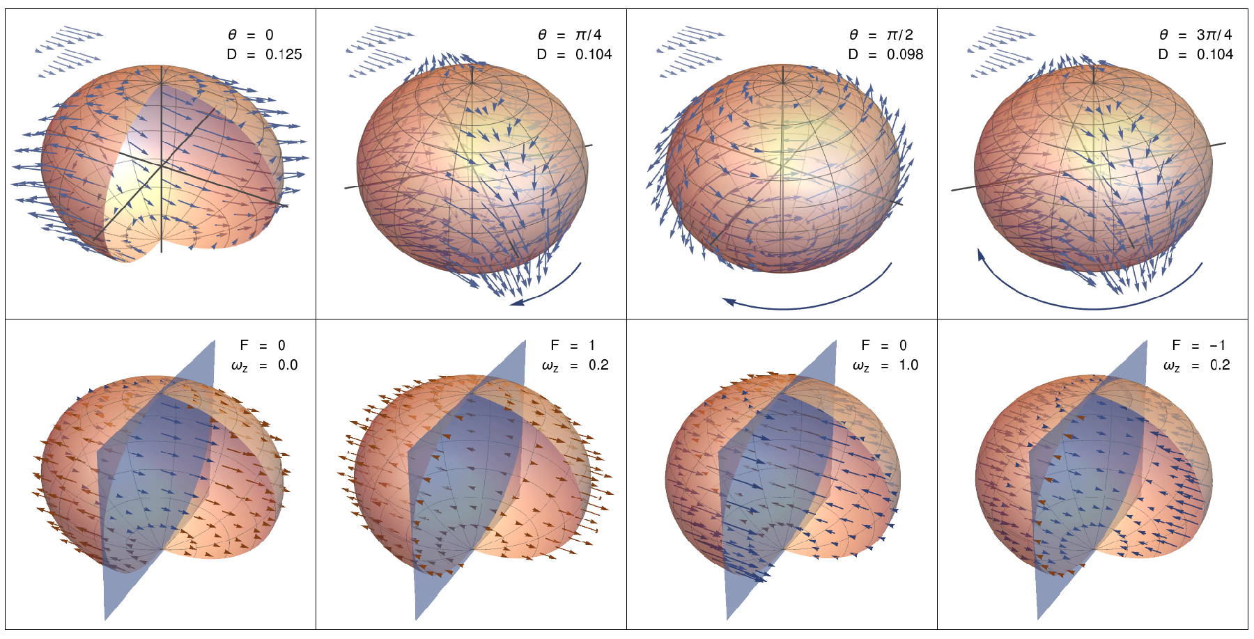
Figure 1: A sample ellipsoid shown at four characteristic time points. The ellipsoid is undergoing periodic tumbling with mild deformation. First row: view from an external reference frame, with surface forces and flow field. $D=(a_{1}-a_{3})/(a_{1}+a_{3})$ is the Taylor deformation parameter , $\theta$ is the angle through which the ellipsoid has rotated. Second row: view from the ellipsoid reference frame, with components of the surface force acting to push into (blue) and pull against (red) a sample fragmentation plane. $F$ is the relative fragmentation force with respect to the plane, and $\omega_{z}$ is the relative angular velocity.

II.5 Parameters of the models

The model parameters are described in Table 1. The DCM depends upon the initial axes lengths $a_{i}$ of the ellipsoid, the velocity gradient $\mathbf{L}$, the matrix viscosity $\mu$, the viscosity ratio $\lambda$, which is the ratio of the droplet viscosity over the matrix viscosity, and the interfacial tension $\Gamma.$ The FCM depends upon the axes lengths $a_{i}(t)$ at each time point, the angular velocity of the ellipsoid $\boldsymbol{\omega}(t)$, and the velocity gradient $\mathbf{L}(t)$, which now also has a dependence on time due to the rotating frame of reference.

Symbol	Parameter	Model	Range	Units
$\mathbf{a}(t)$	axes lengths	D, F	1-1000$\times 10^{-6}$	m
$\boldsymbol{\omega}(t)$	angular velocity	F	0-100	1/s
$\mathbf{L}(t)$	velocity gradient	D, F	0-10	1/s
$\mu$	matrix viscosity	D, F	$8.95\times 10^{-4}$	Pa s
$\lambda$	viscosity ratio	D	1-1000	-
$\Gamma$	interfacial tension	D	$10^{-9}-10^{-7}$	N / m

Table 1: Model parameters.

III Results

III.1 Deformation constituent model

An ellipsoid evolving according to the DCM follows one of three characteristic behaviors: it can (1) collapse smoothly to a steady-state orientation and shape (Fig 2a), (2) collapse while oscillating to a steady-state orientation (Fig 2b), or (3) oscillate periodically (Fig 2c). The angular velocity of the oscillating collapse (Fig 2b) can often exhibit a sudden “flip” in which the direction of rotation of the ellipsoid changes. This occurs when two of the axes lengths are close in magnitude. This interesting behavior will be the topic of future research, and in the remainder of the present work we restrict ourselves to the case of periodic tumbling.

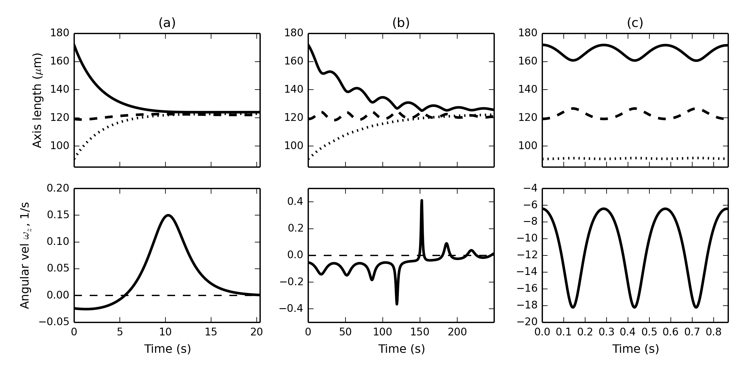
Figure 2: Characteristic behaviors of ellipsoids evolving in the DCM: (a) collapse (Ca$\sim.294$), (b) oscillating collapse (Ca$\sim 13.2$), and (c) periodic tumbling (Ca$\sim 3441$).

In the oscillatory regime shown in Fig 2c, the behavior of the deforming ellipsoid approaches that of a solid ellipsoid. In simple shear defined by $d\mathbf{u}/dy=\dot{\gamma}$, the angle $\theta(t)$ in the $xy$ plane of a solid ellipsoid is given (Yarin et al. (1997) c.f. Blaser (2002)) by

$$\theta_{solid}(t)=-\arctan\frac{a_{1}}{a_{2}}\tan\left(\frac{2\pi t}{T}\right)$$ (11)

where

$$T=\frac{2\pi(a_{1}^{2}+a_{2}^{2})}{a_{1}a_{2}\dot{\gamma}}$$ (12)

is the period of the rotation. From this we can compute the angular velocity component $\omega_{z}$ as

$$\omega_{z,solid}=-\frac{2\pi}{T}\frac{a_{1}a_{2}\sec^{2}\left(2\pi t/T\right)}{a_{2}^{2}+a_{1}^{2}\tan^{2}\left(2\pi t/T\right)}.$$ (13)

In the limit $\lambda\to\infty$, a fluid droplet becomes a solid, in which case we expect tthat the axes lengths will become constant and the angular velocity computed using equation (8) will approach that given in equation (13). This is indeed what we observe; as the viscosity ratio increases, the axis length oscillations decrease (Figure 3a) and the angular velocity converges to that of a solid ellipsoid (Figure 3b).

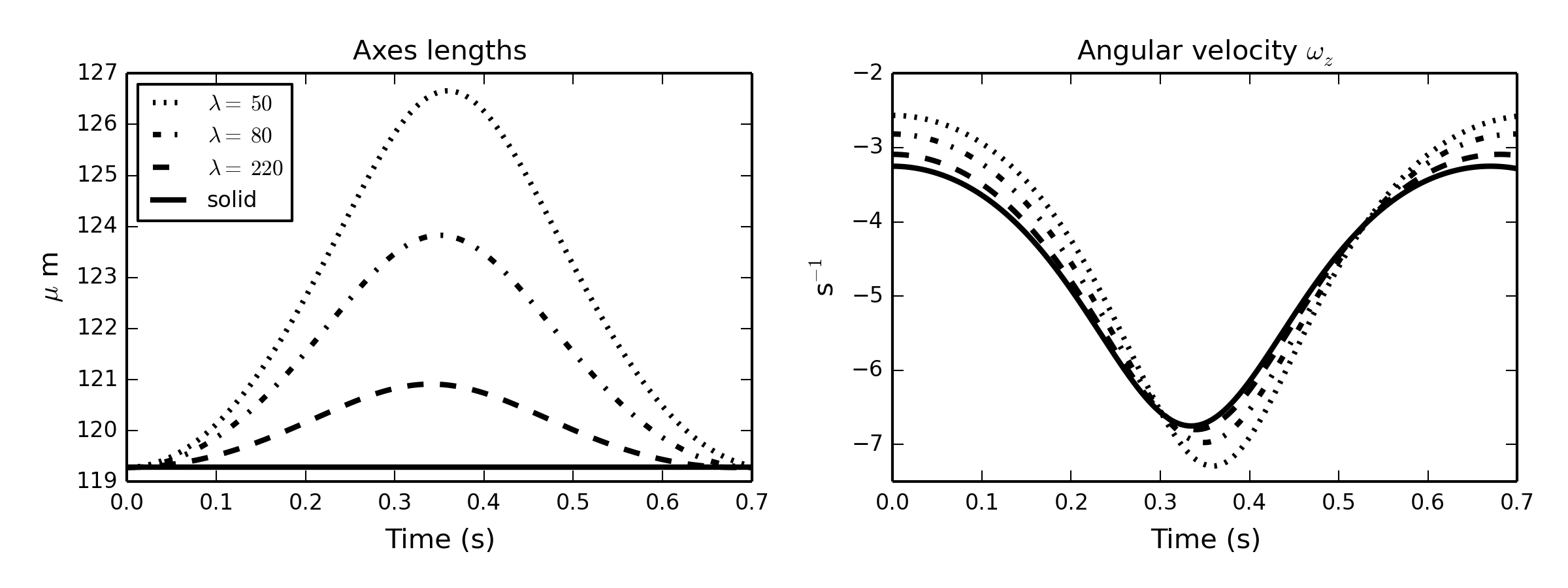
Figure 3: Asymptotic behavior of the DCM as $\lambda\to\infty$ (dashed lines) compared to the behavior of a solid ellipsoid with angular velocity given by equation (13) (solid line). Left: second axis length ($a_{2})$ over time, right: angular velocity component $\omega_{z}$ over time.

III.2 Fragmentation force

Figure (1) shows the evolution in time of a generic ellipsoid at four time-points, including the surface force density as well as the component of this density acting normal to a sample fragmentation plane. This ellipsoid is undergoing periodic tumbling, as in Figure (2)c, with mild deformation. In the first frame, at the initial time, we observe that the surface force density points both outwards and inwards. This feature is responsible for the fact that at the third time point, when the angular velocity is maximized which in turn causes the surface force density magnitudes to be maximized, we nevertheless observe a net fragmentation force of 0. The maximum fragmentation force is observed at the second time-point, when all of the force vectors act against the plane, and the minimum, which is negative, occurs at the fourth time point, when all of the surface force vectors push into the plane.

We examine the behavior of the fragmentation force on a generic ellipsoid $\mathcal{E}$. We intersect $\mathcal{E}$ with a plane $P$ defined by the normal $\mathbf{n}_{p}=(1,0,0)$ and interior point $\mathbf{x}_{p}=(0,0,0)$; i.e., a plane in the $yz$ plane passing through the origin and normal to the longest major axis of $\mathcal{E}$. We first explore the dependence of the fragmentation force, equation (9), on the system parameters. We compute the maximum fragmentation force as a function of the shear rate $\dot{\gamma}$, the viscosity ratio $\lambda$ (which we vary while holding the matrix viscosity $\mu$ constant, changing only $\mu^{*}$), and the interfacial tension $\Gamma$. As can be seen in Figure 4(a), the fragmentation force increases with the shear rate. The shear rate appears directly in the computation of the surface force density in equation 3, and indirectly as it affects the angular velocity $\boldsymbol{\omega}$. At higher shear rates there is a greater dependence of $f_{max}$ on the viscosity ratio, and its dependence on $\lambda$ is non-linear, changing more for smaller values of $\lambda$ while being constant at higher values of $\lambda$. The dependence of $f_{max}$ on $\Gamma$ and $\lambda$ is shown in Figure 4(b). Again, $f_{max}$ increases with $\lambda$; in addition, it can be seen to decrease with $\Gamma$. Neither of these terms appear directly in the force equation (3), and so their influence on $f_{max}$ manifests through their role in shaping the motion and deformation of the ellipsoid as in equation 2.

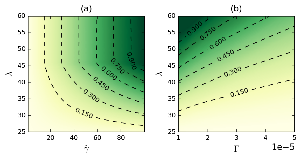
Figure 4: Maximum normalized fragmentation force experienced by a sample ellipsoid as a function of the shear rate $\dot{\gamma}$ and the viscosity ratio $\lambda$ (a) and the interfacial tension $\Gamma$ and the viscosity ratio (b). In (a), $\Gamma=4\times 10^{-9}$ N/m, and in (b) $\dot{\gamma}=10$ m/s.

We next consider the fragmentation force as a function of time and position of the intersecting plane. We construct the ellipsoid as above, except that now we will slide the intersecting plane along the $x$ axis. These results are shown in Figure 5. The $x$ axis corresponds to the position of the interior point on the intersecting plane, so that at a point $x$ on this axis, the intersecting plane is defined by normal $\mathbf{n}_{p}=(1,0,0)$ and $\mathbf{x}_{p}=(x,0,0)$. The $y$ axis corresponds to time. The fragmentation force is anti-symmetric about its horizontal center, which corresponds to the point in time at which the ellipsoid has rotated through an angle of $\pi/2$. Past this point, the symmetry of the system results in the surface forces being equal in magnitude but opposite in sign. As the plane slides along the $x$ axis to the midpoint, the fragmentation force increases, and then decreases again as the plane moves from the center to the other end; again due to the symmetries of the system.

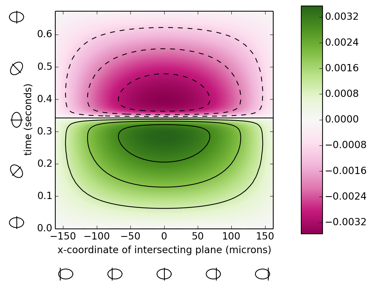
Figure 5: Fragmentation force experienced by a sample ellipsoid deforming according to the DCM, as a function of time ($y$ axis) and the position of the intersecting plane ($x$ axis). In this simulation, $\dot{\gamma}=1$ 1/s, $\lambda=50$, $\mu=8.953\times 10^{-4}$ Pa s, and $\Gamma=4.1\times 10^{-9}$ N/m. Initial ellipsoid axes are $\mathbf{a}=(180,160,140)\mu$m.

IV Conclusion

We presented a unification of theories used to describe the deformation of a fluid droplet and the surface forces on a solid ellipsoid in shear flow. We investigated the qualitative behavior of the forces on the droplet and its motion, and compared this behavior to the simpler case of a solid ellipsoid. We introduced the concept of a fragmentation force, which is the integral of the component of the surface force density acting against an intersecting plane, and saw how this force responds to the placement of the intersecting plane and to the deformation and motion of the droplet. We intend to use the model developed here to simulate the fragmentation of microbial aggregates; in so doing, we will extend our previous work Byrne et al. (2011) by permitting the aggregates to deform and by using the more sophisticated definition of fragmentation force that we have developed here. We expect the work herein to be applicable more generally to simulations of colloidal breakage in which it is desirable to preferentially choose breakage locations, for example in the case of inhomogenous composition. Code for this work (Python and C) is available on GitHub at https://github.com/MathBioCU/fragforce.