Dipole modes with depressed amplitudes in red giants are mixed modes

Abstract

Context. Seismic observations with the space-borne Kepler mission have shown that a number of evolved stars exhibit low-amplitude dipole modes, which are referred to as depressed modes. Recently, these low amplitudes have been attributed to the presence of a strong magnetic field in the stellar core of those stars.

Aims. We intend to study the properties of depressed modes in evolved stars, which is a necessary condition before concluding on the physical nature of the mechanism responsible for the reduction of the dipole mode amplitudes.

Methods. We perform a thorough characterization of the global seismic parameters of depressed dipole modes and show that these modes have a mixed character. The observation of stars showing dipole mixed modes that are depressed is especially useful for deriving model-independent conclusions on the dipole mode damping.

Results. Observations prove that depressed dipole modes in red giants are not pure pressure modes but mixed modes. This result invalidates the hypothesis that the depressed dipole modes result from the suppression of the oscillation in the radiative core of the stars. Observations also show that, except for the visibility, the seismic properties of the stars with depressed modes are equivalent to those of normal stars.

Conclusions. The mixed nature of the depressed modes in red giants and their unperturbed global seismic parameters carry strong constraints on the physical mechanism responsible for the damping of the oscillation in the core. This mechanism is able to damp the oscillation in the core but cannot fully suppress it. Moreover, it cannot modify the radiative cavity probed by the gravity component of the mixed modes. The recent mechanism involving high magnetic field proposed for explaining depressed modes is not compliant with the observations and cannot be used to infer the strength and the prevalence of high magnetic fields in red giants.

1 Introduction

Asteroseismic observations by the CoRoT and Kepler space-borne missions have provided new insights in stellar and Galactic physics (e.g., Michel et al., 2008; Miglio et al., 2009; Chaplin et al., 2011). The ability to derive fundamental stellar parameters such as masses and radii over a wide range of stellar evolutionary states from the main sequence to the asymptotic giant branch is certainly one of the strongest impacts (e.g., Kallinger et al., 2010). The rich nature of the red giant oscillation spectrum was largely unexpected (De Ridder et al., 2009; Mosser & Miglio, 2016). Red giant asteroseismology has been boosted by the observation of dipole modes that, due to their mixed nature, probe the stellar core. They behave as gravity modes in the core and as pressure modes in the envelope. The pressure components carry information on the mass and radius of stars (e.g., Mosser et al., 2013), while the gravity components of these mixed modes are directly sensitive to the size and mass of the helium core (Montalbán & Noels, 2013; Lagarde et al., 2016), to the evolutionary stage differing by the nuclear reaction at work (Bedding et al., 2011; Mosser et al., 2011), and to the mean core rotation (Beck et al., 2012; Mosser et al., 2012b; Deheuvels et al., 2012, 2014).

Due to the homology of the red giant interior structure, red giant seismology is characterized by the many scaling relations between global seismic parameters along stellar evolution (e.g., Stello et al., 2009; Mosser et al., 2010; Mathur et al., 2011; Kallinger et al., 2012). Exceptions to these relations are rare and most often explained by specific features, as for instance the damping of the oscillation in close binaries (Gaulme et al., 2014) or very low metallicity (Epstein et al., 2014). However, observations have revealed that a family of red giants exhibit peculiar dipole modes with low amplitudes (Mosser et al., 2012a). In some extreme cases, dipole modes are not even detectable. Consequently, these dipole modes have been called depressed modes.

The first in-depth study of a star with depressed modes could not explain this phenomenon (García et al., 2014). Then, Fuller et al. (2015) addressed this issue by using a twofold approach. First, the authors expressed the dipole mode visibilities in the limit of full suppression of the oscillation in the red giant core. In other words, they assumed that the mode energy that leaks in the radiative interior of red giants is totally lost. As a consequence, dipole modes are no longer mixed modes but only lie in the upper (acoustic) cavity of red giants. This assumption is validated by the authors by means of a comparison between observed and computed mode visibilities. Second, it is conjectured that the extra loss of the mode energy is caused by a strong magnetic field, which scatters waves leaking in the core. This prevents them from constructing a standing wave in the inner resonant cavity of those stars. This has been named as the magnetic greenhouse effect. The angular degree dependence of the energy leakage has been verified with the quadrupole modes (Stello et al., 2016a). This appealing scenario has then been taken as granted by Stello et al. (2016b) and Cantiello et al. (2016) to infer the prevalence of magnetic fields in the core of oscillating red giant stars observed by Kepler.

However, before firmly concluding about the presence of a magnetic field in the core of red giants with depressed modes, the hypothesis of the suppression of the oscillation in the core has to be validated. In fact, the nature of the physical mechanism responsible for the reduction of dipole mode visibilities is not directly inferred by the observation of low mode visibilities. Therefore, the identification of a magnetic field as the physical mechanism responsible for the suppression of the oscillation in the core of those stars demands further direct observational confirmations. A strong magnetic field is a possible solution, but not the only one. Fuller et al. (2015) note that rapid core rotation should have the same effect, but would require much larger rotation rates than observed in red giants (Mosser et al., 2012b; Deheuvels et al., 2014). Indeed, any strong damping in the core such as radiative damping or gravity wave reflection, caused for instance by a steep composition gradient above the hydrogen burning shell, could also explain the depressed modes (Dziembowski, 2012).

In this work, we aim at providing a complete characterization of the population of red giants with depressed modes, using Kepler observations. This study is motivated by the observation of stars showing dipole modes that are both mixed and depressed. We argue that the full characterization of stars with depressed visibilities can provide strong constraints on the physical mechanism responsible for the damping of the oscillation.

The article is organized as follows. Section 2 presents the theoretical background of mode visibility, with an emphasis on the distinction between full and partial mode damping in the core of red giants. In Section 3, we undertake the characterization of depressed modes with a mixed character, hereafter named depressed mixed modes. We first explain how they were identified, then exploit their observations with the determination of their global seismic properties. We also consider stars where, owing to the too low visibility of dipole modes, the gravity-dominated mixed modes are apparently absent. Global properties of stars are then used to test the depressed visibilities predicted when the oscillation is suppressed in the stellar core (Section 4). Section 5 is devoted to discussion, with particular attention to the nature of the mechanism responsible for the extra-damping of depressed modes. Finally, Section 6 is dedicated to conclusions.

2 Dipole mode visibilities

2.1 General case

The mode visibility is a way to express the mean value of the squared amplitude of modes with a given degree compared to radial modes. For a dipole mode, we define

$$V_{1}^{2}={A_{1}^{2}\over A_{0}^{2}}\ \tilde{V}_{1}^{2},$$ (1)

where $\tilde{V}_{1}^{2}$ includes the contributions of several physical effects: a geometrical factor that depends on the angular degree, the limb-darkening, and the bolometric correction. $A_{0}$ and $A_{1}$ are the intrinsic amplitudes of the radial and dipole modes, respectively. For stars exhibiting stochastically excited pure acoustic modes, these amplitudes are supposed to be equal (Belkacem et al., 2008). In such a case, the visibility $V_{1}^{2}$ reduces to $\tilde{V}_{1}^{2}$.

A simple way to address the depressed modes consists in normalizing the dipole visibility with respect to the nominal expected value. We therefore use the same definition as Fuller et al. (2015) for expressing the relative visibility of depressed modes. In a first step, we consider the individual visibilities of the mixed modes

$$v_{{n_{\mathrm{m}}}}={{V_{1}^{2}}_{\mathrm{depressed}}\over\tilde{V}_{1}^{2}}.$$ (2)

where the mixed order ${n_{\mathrm{m}}}$ labels the mixed mode (Eqs. (4.60)-(4.63) of Mosser, 2015). Strictly speaking, $v_{{n_{\mathrm{m}}}}$ should be referred to as a ratio of the squared amplitudes of dipole modes compared to radial modes, since the contribution of the different visibility terms (aspect ratio of the spherical harmonics and limb-darkening coefficients) is removed by the ratio to $\tilde{V}_{1}^{2}$. However, we keep the term visibility for the sake of simplicity.

For red giants, Ballot et al. (2011) computed $\tilde{V}_{1}^{2}\simeq 1.54$, assuming that only acoustic modes are present. In evolved stars, the situation is in fact complicated by the mixed modes. The contribution of all mixed modes associated with a given pressure radial order ${n_{\mathrm{p}}}$ can be expressed as

$$v=\sum_{{n_{\mathrm{m}}}\in\{{\mathcal{N}}\}}v_{{n_{\mathrm{m}}}}.$$ (3)

The sum is made in the ensemble $\{{\mathcal{N}}\}$ of the ${\mathcal{N}}$ mixed modes associated with a given pressure radial order. They lie in the $\Delta\nu$-wide frequency range between two radial modes: for the pressure radial order around $\nu_{\mathrm{max}}$, ${\mathcal{N}}=\Delta\nu\Delta\Pi_{1}^{-1}\nu_{\mathrm{max}}^{-2}$, where $\Delta\nu$ is the mean large separation of pressure modes, $\Delta\Pi_{1}$ is the period spacing of gravity modes, and $\nu_{\mathrm{max}}$ is the frequency of maximum oscillation signal.

The mixed-mode visibility $v_{{n_{\mathrm{m}}}}$ introduced by Eq. (2) has been investigated in previous work (Dupret et al., 2009; Benomar et al., 2014; Grosjean et al., 2014), which shows

$$v_{{n_{\mathrm{m}}}}\simeq\left(\frac{\Gamma_{0}}{\Gamma_{n_{\mathrm{m}}}}\right)\left(\frac{I_{0}}{I_{n_{\mathrm{m}}}}\right)^{2},$$ (4)

where $\Gamma_{0},\Gamma_{n_{\mathrm{m}}}$ ($I_{0},I_{n_{\mathrm{m}}}$) are the linewidths (inertia) of the radial and dipole modes, respectively. This equation is valid whenever the dipole mode is resolved or not, but assumes that the driving is the same for radial and dipole modes. To go further, we have to examine two cases, depending on the assumption on the dipole modes.

2.2 Normal dipole mixed modes

Following Belkacem et al. (2015), we may consider that the work performed by the gas during one oscillation cycle, associated with surface damping, is the same for all modes, so that Eq. (4) is simplified into

$$v_{{n_{\mathrm{m}}}}\simeq{I_{0}\over I_{n_{\mathrm{m}}}}\simeq{\Gamma_{n_{\mathrm{m}}}\over\Gamma_{0}},$$ (5)

from which we retrieve that the individual visibilities of mixed modes are small, with smaller mode widths and larger inertia than radial modes.

From observations, Mosser et al. (2012a) have shown that the contribution of all mixed modes associated with a given pressure radial order ${n_{\mathrm{p}}}$ ensures $v=1$. Here, we can demonstrate this, using the relation between inertia and the function $\zeta$ that governs the mixed-mode spacings and the rotational splittings (Goupil et al., 2013; Deheuvels et al., 2015; Mosser et al., 2015). From $I_{0}/I_{n_{\mathrm{m}}}=1-\zeta$, we have

$$v=\sum_{{n_{\mathrm{m}}}\in\{{\mathcal{N}}\}}(1-\zeta).$$ (6)

The ${\mathcal{N}}$ mixed modes in the ensemble $\{{\mathcal{N}}\}$ between two consecutive radial modes correspond to 1 pure pressure dipole mode and $({\mathcal{N}}-1)$ pure gravity dipole modes. The period difference between the two radial modes can be estimated in two ways, either considering the sum $({\mathcal{N}}-1)\,\Delta\Pi_{1}$ for the pure gravity modes, or considering the sum of the mixed-mode period spacings: $\sum_{{n_{\mathrm{m}}}\in\{{\mathcal{N}}\}}\Delta P=(\sum_{{n_{\mathrm{m}}}\in\{{\mathcal{N}}\}}\zeta)\;\Delta\Pi_{1}$, according to Mosser et al. (2015). Hence, we get

$$v=\sum_{{n_{\mathrm{m}}}\in\{{\mathcal{N}}\}}(1-\zeta)={\mathcal{N}}-({\mathcal{N}}-1)=1.$$ (7)

This result proves that, despite the mixed nature of the dipole modes, their total visibility matches the expected visibility of the corresponding pure pressure mode. So, energy equipartition is preserved for the normal mixed modes.

2.3 A particular case: suppression of the oscillation in the core

The possibility of the suppression of the oscillation in the core was first investigated by Unno et al. (1989). Their equations (16.62)-(16.65) consider the effect of a wave leakage in the core of an acoustic mode trapped in the convective envelope. The limit of oscillation suppression in the core implies that only pressure dipole modes are present since mixed modes are necessarily cancelled out. In that case, $I_{1}\simeq I_{0}$, so that Eq. (4) rewrites

$$v={\Gamma_{0}\over\Gamma_{1}}.$$ (8)

The damping in the core, whatever it is, can be written

$$v=\frac{\Gamma_{0}}{\Gamma_{1}^{\rm env}+\Gamma_{1}^{\rm core}}\simeq\frac{\Gamma_{0}}{\Gamma_{0}+\Gamma_{1}^{\rm core}},$$ (9)

where $\Gamma_{1}^{\rm env}\simeq\Gamma_{0}$ and $\Gamma_{1}^{\rm core}$ are the damping contributions in the envelope and in the core, respectively.

2.3.1 Damping and transmission

Equation (9) can be rewritten

$$v=\frac{1}{1+x}\quad{\rm with}\quad x=\frac{\Gamma_{\rm 1}^{\rm core}}{\Gamma_{0}}.$$ (10)

When all energy transmitted in the core is absorbed or damped, following Unno et al. (1989) we get

$$x=\omega\tau_{\mathrm{a}}\left(\int_{\mathcal{A}}k_{r}\,\mathrm{d}r\right)^{-1}\frac{1}{4}\exp\left(-2\int_{\mathcal{E}}\kappa\,\mathrm{d}r\right),$$ (11)

where ${\mathcal{A}}$ denotes integration in the acoustic cavity and ${\mathcal{E}}$ in the evanescent region, $k_{r}$ is the radial wave number, $\kappa^{2}=-k_{r}^{2}$, $\omega$ is the mode frequency, and $\tau_{\mathrm{a}}$ is the e-folding damping time of the radial mode amplitude. At first order, the first integral of Eq. (11) equals $\omega/2\Delta\nu$, where $\Delta\nu$ is the large separation. Thus, Eq. (11) becomes

$$x=\frac{\Delta\nu\,\tau_{\mathrm{a}}}{2}\exp\left(-2\int_{\mathcal{E}}\kappa{\rm d}r\right).$$ (12)

We then introduce the e-folding damping time of the mode energy, $\tau_{0}=\tau_{\mathrm{a}}/2$ and get

$$v=\left(1+\Delta\nu\,\tau_{0}\,T^{2}\right)^{-1},$$ (13)

where the transmission in the evanescent region is defined by

$$T=\exp\left(-\int_{\mathcal{E}}\kappa{\rm d}r\right).$$ (14)

Equation (13), derived from the relative visibility of depressed dipole modes with respect to radial modes, is similar to Eq. (2) of Fuller et al. (2015), derived from the ratio between the depressed and normal dipole modes.

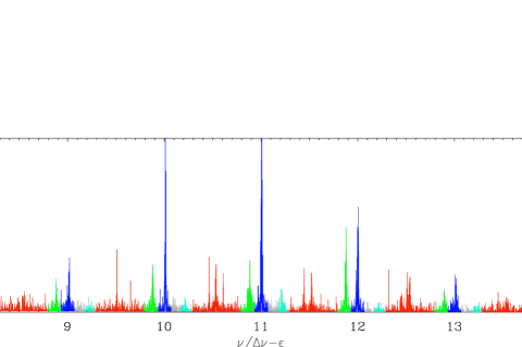
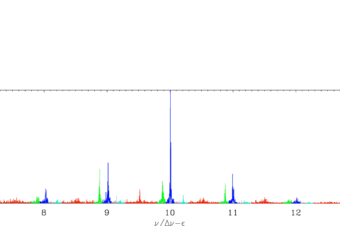
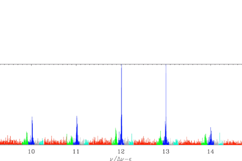
Figure 1: Examples of RGB stars with low dipole-mode amplitudes. Spectra are plotted as a function of the reduced frequency $\nu/\Delta\nu-\varepsilon$, so that radial modes (shown in blue) are close to integer values; quadrupole modes are plotted in green, octupole modes in cyan; mixed modes can be found everywhere but their contribution is measured in the frequency range plotted in red only. The mean background component was subtracted. top) the mixed mode pattern of KIC 9279486 can be fitted in order to extract seismic global parameters; middle) mixed modes in KIC 6026983 are evidenced but their pattern cannot be fit; bottom) dipole modes of KIC 5810513 have very small amplitudes but can be unambiguously detected and identified as mixed modes with the method discussed in Section 3.3.

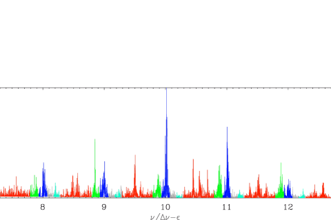
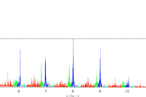
Figure 2: Same as Fig. 1 but for core-helium burning stars. top) the mixed mode pattern of the secondary-clump star KIC 8522050 can be fitted in order to extract seismic global parameters; bottom) depressed mixed modes in the clump star KIC 2693261 are apparent but their pattern cannot be fit.

2.3.2 Link with observable parameters

We can match the value of $T^{2}$ with the coupling factor $q$ of mixed modes (Unno et al., 1989):

$$T^{2}=4q.$$ (15)

The visibility can thus be expressed as a function of the seismic observables $q$ and $\Gamma_{0}$

$$v=\left(1+2q\ {\Delta\nu\over\pi\Gamma_{0}}\right)^{-1}.$$ (16)

The coupling factor $q$ is obtained from the asymptotic expansion of mixed modes

$$\tan\theta_{\mathrm{p}}=q\tan\theta_{\mathrm{g}},$$ (17)

where the phases $\theta_{\mathrm{p}}$ and $\theta_{\mathrm{g}}$ refer, respectively, to the pressure- and gravity-wave contributions (Mosser et al., 2015). The radial mode width $\Gamma_{0}$, measured as the full width at half maximum in the power density spectrum, is related to the radial mode lifetime by (see Samadi et al., 2015)

$$\Gamma_{0}={1\over 2\pi\tau_{0}}.$$ (18)

In fact, Eqs. (15) and (16) are no longer valid when the extent of the evanescent region is limited, so that strong coupling occurs. In that case (see Takata, 2016a),

$$T^{2}={4q\over(1+q)^{2}}.$$ (19)

Following Eq. (71) of Takata (2016b), we also have to replace $T^{2}$ by $-\ln(1-T^{2})$ in case of full suppression of the oscillation in the core. So, Eq. (13) becomes

$$v=\left(1-\ln\left[1-{4\,q\over(1+q)^{2}}\right]{\Delta\nu\over 2\pi\Gamma_{0}}\right)^{-1}.$$ (20)

Contrary to Eq. (13), this expression ensures a null visibility in case of total transmission ($T=q=1$).

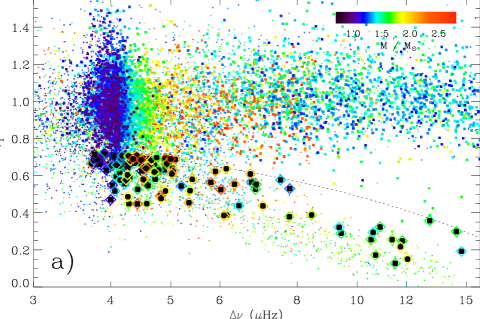
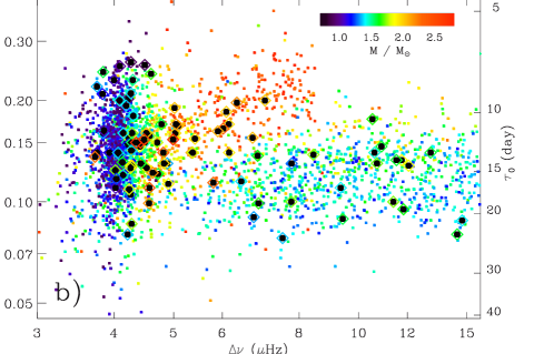
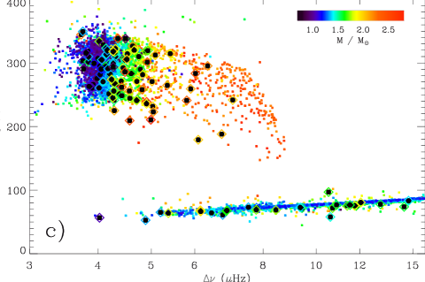
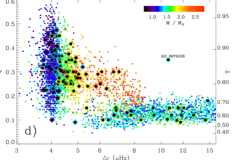
Figure 3: a) Dipole mode visibility $v_{1}$ as a function of the large separation $\Delta\nu$. The color codes the mass, determined with seismic scaling relations. Small symbols represent Kepler stars of the public data set; larger symbols represent stars of the data set studied by Vrard et al. (2016). Diamonds with a dark center are stars showing depressed mixed modes. The dashed line represents the limit defining low visibilities; b) Radial mode width $\Gamma_{0}$ as a function of the large separation $\Delta\nu$ of the data set studied by Vrard et al. (2016). The right y-axis provides the radial mode lifetime; c) Same as b) for the period spacings $\Delta\Pi_{1}$; d) Same as b) for the coupling factor $q$. The outlying value of $q$ for KIC 6975038 is discussed in Section 5.4.

3 Seismic observables

Previous observations have reported that the depressed modes in the red giant KIC 8561221 are mixed (García et al., 2014). Such observations question the hypothesis of oscillation suppression: if the low visibility derives from the suppression of the oscillation in the radiative core, mixed modes cannot be established. Therefore, we first aim at identifying the prevalence of red giants with depressed mixed modes. Then, we also use different observations to assess the properties of depressed dipole modes, in order to determine whether they are mixed or not. Figure 1 illustrates the different types of stars we intend to work with: either with depressed mixed modes that can be identified, or with depressed mixed modes that cannot be fitted, or without clear evidence of mixed modes. Figure 2 provides examples for core-helium burning stars.

3.1 Identification of low visibilities

The first step for the search of stars with dipole mixed modes consists in the measurement of reduced visibilities, as defined by Eq. (3), with the method of Mosser et al. (2012a). In short, squared amplitudes are estimated from the integration of the power spectrum density over the frequency range covering the different modes, after subtraction of background. We obtained the total dipole visibilities $V_{1}^{2}$ for about 12 500 red giants of the Kepler public data (Fig. 3a), from which we could identify the population of stars on the red giant branch (RGB) with normal visibilities and the family of stars with low visibility, in agreement with Mosser et al. (2012a) and Stello et al. (2016a). Red giants with normal amplitudes have a total dipole visibility close to $\tilde{V}_{1}^{2}\simeq 1.54$, with a very small dependence in $T_{\mathrm{eff}}$, $\log g$ and $Z$. Using effective temperatures of Huber et al. (2014), we found that the normal (not depressed) visibilities of red giants, integrated for one pressure radial order, follow the mean trend

$$\langle\tilde{V}_{1}^{2}\rangle\simeq 1.54-{T_{\mathrm{eff}}-4850\over 4100},$$ (21)

where the brackets indicate the average value derived from a linear fit with the effective temperature $T_{\mathrm{eff}}$ expressed in kelvin. We note that this result is very close to the predictions of Ballot et al. (2011).

The mean value of the normal visibility was then used to derive reduced integrated observed visibilities

$$v_{1}={\overline{\sum V_{1}^{2}}\over\langle\tilde{V}_{1}^{2}\rangle},$$ (22)

where, for the numerator, the sum matches all dipole modes associated to a given pressure radial order and the overbar represents the mean value for the different radial orders where dipole modes are observed. Now, $v_{1}$ can be compared to $v$ (Eq. 3). As stated by previous work, the limit between normal and low visibility is clear on the RGB, despite the presence of a few stars lying in the no man’s land between normal and reduced visibilities; in the red clump, we chose to define low-visibility stars by $v_{1}\leq 0.85-0.04\,\Delta\nu$ (with $\Delta\nu$ expressed in $\mu$Hz). We tested that changing the threshold value does not significantly change the conclusions of the work.

Table 1: Seismic properties of $71$ stars showing depressed mixed modes

KIC	evolutionary	$\nu_{\mathrm{max}}$	$\Delta\nu$	$\Delta\Pi_{1}$	$q$	$M$	$\Gamma_{0}$	$\delta\nu_{\mathrm{rot}}$	$v_{1}$	$v$	$v$
	stage	($\mu$Hz)	($\mu$Hz)	(s)		($M_{\odot}$)	($\mu$Hz)	(nHz)		low	strong
	(1)				(2)		(3)	(4)
2573092	RC	35.3	4.08	293.8	0.24	1.48	0.14	35	0.60	0.181	0.178
2858129	RC2	40.5	4.22	320.9	0.26	1.93	0.16	80	0.58	0.181	0.178
2992350	RC	45.9	4.72	242.8	0.26	1.59	0.12	35	0.58	0.134	0.132
3443483	RGB	132.2	10.71	71.8	0.15	1.71	0.13	230	0.16	0.113	0.112
3532734	RGB	145.2	11.83	75.3	0.12	1.63	0.09	0	0.23	0.095	0.095
3660245	RC	33.3	4.22	297.0	0.25	1.19	0.15	35	0.65	0.181	0.178
3758505	RGB	157.4	12.06	80.6	0.15	1.84	0.13	500	0.14	0.100	0.099
4180939	RC2	65.2	5.80	241.0	0.24	2.29	0.11	50	0.55	0.114	0.112
4587050	RGB	191.2	14.47	73.8	0.10	1.60	0.08	530	0.26	0.080	0.080
4761301	RC	30.8	4.49	338.3	0.30	0.76	0.25	65	0.63	0.229	0.224
4772722	RC	37.3	4.30	310.0	0.31	1.42	0.18	38	0.67	0.175	0.170
5007332	RGB	96.9	8.44	68.7	0.10	1.76	0.14	310	0.37	0.204	0.204
5179471	RC2	47.0	4.56	256.0	0.28	2.17	0.10	110	0.64	0.109	0.106
5295898	RGB	142.9	11.39	75.3	0.10	1.72	0.10	210	0.23	0.123	0.123
5306667	RC	39.5	4.28	268.0	0.28	1.77	0.14	25	0.67	0.158	0.154
5339823	RC	40.4	4.28	317.2	0.45	1.76	0.16	80	0.45	0.115	0.108
5620720	RC2	57.0	5.35	264.7	0.29	2.14	0.14	45	0.45	0.124	0.121
5881079	RGB	67.2	6.14	68.3	0.10	1.96	0.17	0	0.62	0.303	0.302
5949964	RC	37.8	4.29	316.3	0.35	1.50	0.23	40	0.59	0.194	0.187
6037858	RC	43.3	4.57	244.4	0.25	1.76	0.16	50	0.45	0.178	0.174
6130770	RC	35.1	4.13	322.9	0.30	1.48	0.12	40	0.62	0.132	0.128
6210264	RC	40.7	4.78	290.0	0.25	1.60	0.17	60	0.63	0.183	0.180
6232858	RC2	50.0	4.90	235.8	0.28	1.87	0.11	55	0.51	0.115	0.112
6610354	RC2	46.9	4.57	209.3	0.28	2.44	0.11	65	0.55	0.119	0.116
6975038	RGB	128.4	10.61	57.9	0.35	1.44	0.14	280	0.27	0.056	0.054
7512378	RC	32.5	3.84	310.0	0.32	1.34	0.16	45	0.70	0.170	0.165
7515137	RGB	67.2	6.75	61.1	0.12	1.32	0.09	0	0.55	0.149	0.148
7693833	RGB	31.8	4.02	56.6	0.10	1.05	0.11	0	0.55	0.301	0.300
7746983	RGB	188.6	14.74	83.3	0.18	1.40	0.09	190	0.17	0.050	0.049
8009582	RC	35.2	4.21	282.4	0.22	1.36	0.08	30	0.56	0.120	0.118
8025383	RC	36.1	4.14	313.5	0.25	1.41	0.16	25	0.58	0.195	0.192
8283646	RGB	67.2	6.15	66.5	0.10	1.93	0.14	100	0.38	0.263	0.263
8391175	RGB	87.4	7.77	69.0	0.12	1.72	0.10	0	0.36	0.144	0.144
8396782	RC2	82.3	7.04	241.8	0.30	2.00	0.20	200	0.42	0.129	0.126
8432219	RC	42.3	4.59	283.2	0.30	1.66	0.24	45	0.55	0.215	0.210
8476202	RGB	109.7	9.42	71.7	0.12	1.57	0.09	0	0.27	0.110	0.110
8522050	RC2	75.5	6.72	188.1	0.30	2.06	0.16	60	0.59	0.108	0.105
8564277	RC	31.9	4.00	307.0	0.31	1.09	0.23	25	0.47	0.226	0.220
8564559	RC	45.8	4.70	240.9	0.25	1.79	0.15	40	0.62	0.167	0.164
8636174	RC2	43.9	4.51	305.7	0.25	2.00	0.16	35	0.58	0.182	0.179
8687248	RGB	170.0	13.10	77.8	0.12	1.59	0.14	0	0.32	0.123	0.122
8689599	RC	30.4	3.93	299.3	0.32	1.17	0.14	35	0.63	0.149	0.144
8771414	RC	38.6	4.23	274.0	0.25	1.82	0.11	28	0.58	0.139	0.137
8827934	RGB	55.0	5.37	63.8	0.15	1.80	0.14	0	0.51	0.214	0.213
9115334	RC2	67.5	6.09	179.2	0.30	2.00	0.19	220	0.38	0.137	0.134
9176207	RC2	59.2	5.41	314.6	0.24	1.96	0.15	100	0.57	0.157	0.154
9229592	RGB	72.0	6.85	67.2	0.15	1.62	0.14	230	0.51	0.173	0.172
9279486	RGB	132.4	10.89	76.8	0.12	1.59	0.15	200	0.30	0.149	0.149
9291830	RC2	47.5	4.41	261.8	0.30	2.50	0.15	70	0.44	0.151	0.147
9581849	RC	34.6	4.08	270.5	0.37	1.43	0.20	30	0.66	0.172	0.165
9650046	RC2	68.2	6.02	283.5	0.25	2.42	0.17	90	0.51	0.147	0.144
9711269	RGB	64.1	6.44	64.2	0.10	1.39	0.12	0	0.43	0.219	0.218
9719858	RC2	47.8	4.48	285.8	0.25	2.62	0.15	90	0.68	0.174	0.171
9947511	RC	30.7	3.75	349.5	0.33	1.35	0.22	30	0.69	0.218	0.212
10029821	RC2	64.6	5.90	259.3	0.29	2.08	0.16	50	0.61	0.129	0.126
10091729	RC2	72.8	6.34	295.3	0.23	2.18	0.20	60	0.54	0.175	0.173
10420655	RC	37.5	4.26	298.6	0.28	1.39	0.21	50	0.64	0.217	0.212
10422589	RC2	50.2	5.04	223.1	0.24	2.15	0.17	60	0.62	0.181	0.178
10469976	RC2	52.7	4.81	258.0	0.30	2.35	0.14	30	0.49	0.132	0.129
10528917	RGB	76.4	7.52	73.1	0.13	1.36	0.08	220	0.56	0.111	0.111
10653383	RC	40.1	4.42	248.5	0.26	1.60	0.13	30	0.53	0.151	0.148
10854564	RC	29.9	4.26	293.5	0.22	0.69	0.26	30	0.66	0.304	0.300
11413158	RC2	58.1	4.99	210.6	0.28	2.86	0.15	80	0.68	0.149	0.146
11462972	RC2	29.9	4.26	318.0	0.26	1.89	0.13	30	0.49	0.154	0.151
11519450	RGB	72.8	6.87	68.1	0.14	1.65	0.10	180	0.54	0.139	0.138
11598312	RC2	48.0	4.82	281.5	0.22	1.96	0.13	50	0.47	0.161	0.159
12058556	RGB	105.0	9.35	72.7	0.15	1.40	0.11	0	0.31	0.110	0.109
12070510	RC	35.3	4.06	304.9	0.23	1.36	0.14	50	0.52	0.191	0.188
12109388	RC	40.9	4.25	245.3	0.26	1.82	0.13	50	0.60	0.152	0.149
12453551	RC2	51.2	5.02	270.8	0.29	2.04	0.19	70	0.60	0.170	0.166
12691734	RC2	46.8	4.34	338.5	0.31	2.73	0.15	50	0.69	0.151	0.147

- (1) RGB: red giant branch; RC: red clump; RC2: secondary red clump.

- (2) Uncertainties on $q$ are of about $\pm$0.027 for stars on the RGB and $\pm$0.057 in the red clump.

- (3) Uncertainties on $\Gamma_{0}$ are of about 30 %.

- (4) A null value for $\delta\nu_{\mathrm{rot}}$ indicates that the rotational splitting could not be measured because the star is seen pole-on.

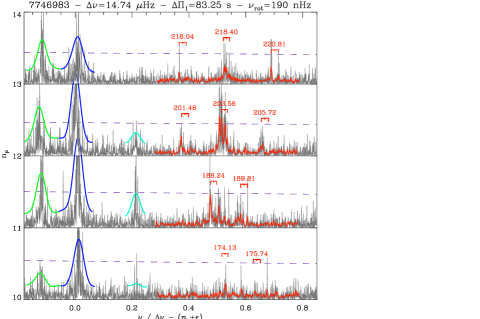
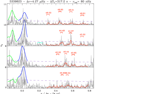
Figure 4: Examples of complete fits of the asymptotic mixed-mode pattern of red giants with low dipole-mode amplitudes. Échelle diagrams are plotted as a function of the reduced frequency $\nu/\Delta\nu-({n_{\mathrm{p}}}+\varepsilon)$, so that radial modes are close to integer values. The smoothed profile of mixed modes are plotted in red, quadrupole modes in green, octupole modes in cyan. The dashed gray line corresponds to 8 time the granulation background. Dipole triplets are identified by the asymptotic cyclic frequency, in $\mu$Hz, of the $m=0$ component. top) RGB star, KIC 7746983; bottom) Clump star, KIC 5339823.

3.2 Fit of the mixed-mode pattern

The systematic search for stars with depressed mixed modes was derived from the recent work of Vrard et al. (2016), who have measured the asymptotic period spacing of mixed modes for about 6 100 red giants. We then fitted the asymptotic mixed-mode pattern in stars with reduced dipole visibilities.

The fit of mixed mode frequencies in red giants is usually made easy by the use of the asymptotic expansion (Unno et al., 1989; Mosser et al., 2012b), but is more difficult in stars with depressed mixed modes because of the lower signal-to-noise ratio induced by the low visibilities. However, we managed to optimize this fitting process to obtain complete sets of seismic parameters, including rotational splittings $\delta\nu_{\mathrm{rot}}$ (Mosser et al., 2012b). Recent methods and results based on four years of Kepler observation were used to update previous measurements (Mosser et al., 2014, 2015; Vrard et al., 2016). Stellar masses were estimated from the seismic scaling relation with the method of Mosser et al. (2013) in order to have a better calibration than the solar calibration and to lower the non-negligible noise induced by pressure glitches (Vrard et al., 2015). Scaling relations have been used with the effective temperature of Huber et al. (2014).

We were able to fit the asymptotic mixed-mode pattern, including the rotational splittings, for $71$ red giants (Table 1, Fig. 4). This number represents a small fraction of the 1109 stars with low amplitudes since fitting all parameters of the asymptotic mixed-mode pattern is highly demanding when amplitudes are depressed. Unsurprisingly, owing to the aforementioned observational bias, our data set with mixed modes on the RGB is biased toward high visibilities (Fig. 3a). Conversely, as low visibilities of clump stars are not as low as on the RGB, fitting their mixed modes is easier. With this analysis, we can establish the properties of stars with depressed mixed modes.

Mass

Stars in our data set with depressed mixed modes present larger masses than the typical mass distribution of CoRoT or Kepler red giants showing solar-like oscillations. Their median mass is 1.6 $M_{\odot}$, above the median mass of the red giants observed with Kepler (1.4 $M_{\odot}$). This agrees with the mass distribution found by Stello et al. (2016b) for stars with low-amplitude dipole modes.

Evolutionary stage

Mosser et al. (2012a) have reported the identification of low visibilities for stars on the RGB. Here, we report that stars with depressed mixed modes appear at any evolutionary stages. We identified depressed modes in secondary-clump stars, located on the same low-visibility branch as RGB stars (Fig. 3a). Due to the mass dependence of the low-visibility stars, depressed modes are in fact over-represented in the secondary red clump. The situation is less clear for clump stars, since the low-visibility branch joins the group of normal visibility stars when $\Delta\nu\leq 4.5\,\mu$Hz. We however notice an overabundance of red-clump stars with low visibilities, much more abundant than stars with visibilities above the normal value. An example of such star is given in Fig. 2 (bottom panel).

Radial mode widths

Radial mode widths $\Gamma_{0}$, defined as full widths as half maximum, were measured following the method used by Vrard et al. (2015). Results are shown in Fig. 3b. They are fully consistent with previous work obtained with CoRoT and Kepler (Baudin et al., 2011; Corsaro et al., 2012, 2015) and show a clear dependence with the evolutionary stage and the stellar mass, as will be discussed in a forthcoming paper. In the clumps, $\Gamma_{0}$ of stars with depressed mixed modes behave as for the other stars. On the RGB, these stars appear to have slightly larger $\Gamma_{0}$ than the mean trend. This is however a mass effect only: $\Gamma_{0}$ increases with increasing masses, and low visibility stars show higher mass (Stello et al., 2016b).

Asymptotic period spacing

Asymptotic period spacings follow the typical distribution identified in previous work (Mosser et al., 2012c, 2014; Vrard et al., 2016). We could not identify any departure to the distribution of the $\Delta\nu$ – $\Delta\Pi_{1}$ relation (Fig. 3c). On the RGB, stars with depressed mixed modes show slightly lower values of $\Delta\Pi_{1}$ than the mean case, in agreement with their mass distribution (Vrard et al., 2016). Values are normal in the red clump. The large mass range and the non-degenerate conditions for helium ignition of secondary red clump stars explains the spread in the distribution of their seismic parameters, so that the spread for stars with depressed modes does not allow to draw any conclusion.

Coupling factors

Coupling factors $q$ were measured by Mosser et al. (2016) for about 4 000 stars among the data set analyzed by Vrard et al. (2016). These factors are derived from the optimization of the method introduced by Mosser et al. (2015) for analyzing mixed modes. Results are shown in Fig. 3d, where stars with a low dipole-mode visibility are identified. We refer to Mosser et al. (2016) for the discussion of the general trends observed in $q$ as a function of the evolutionary stage. Here, we note that stars with depressed modes behave as the other stars. This suggests that the extent of the evanescent region between the pressure and gravity components is not impacted by the mechanism responsible for the amplitude mitigation, so that it is very similar as for normal stars (Unno et al., 1989; Takata, 2016a).

Rotation

Fitting rotation requires a high signal-to-noise ratio in the oscillation spectrum, so that the difficulty of this measurement explains the limited number of stars with a complete fit. It is evidently a bias due to the low visibilities. For the same reason, more fits than expected are obtained for the mixed-mode patterns of stars nearly seen pole-on, which are simpler than the general case since the rotational multiplets are reduced to the zonal modes (with an azimuthal order $m$=0). In such cases, the core rotation remains undetermined. When measured, rotational splittings show the typical distributions defined for red giants (Mosser et al., 2012b; Deheuvels et al., 2014, 2015).

Evolutionary	$\Delta\nu$	$\Gamma_{0}$	$\tau_{0}$
status	($\mu$Hz)	(nHz)	(day)
RGB	15	118$\pm$25	15.5$\pm$3.3
RGB	10	121$\pm$23	15.1$\pm$3.0
RGB	6	118$\pm$30	15.6$\pm$3.9
red clump	4	145$\pm$37	12.6$\pm$3.2
secondary clump	7	178$\pm$45	10.3$\pm$2.6

Table 2: Mean mode width and lifetime (defined as the e-folding time of the mode energy), depending on the evolutionary, for red giants

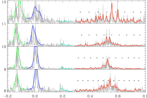
Figure 5: Échelle spectrum of the RGB star KIC 9711269. Colored lines, with the same color code as in Fig. 1, emphasize the structure of the modes. Plus symbols approximately indicate the period spacings derived from the asymptotic expansion; the fit of the mixed modes, which would imply the fit of the rotational splittings, is however not possible.

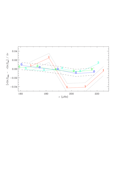
Figure 6: The evidence of dipole mixed modes is provided by the position of low-degree modes with respect to the second-order asymptotic expansion of pure pressure modes, for the red giant 5810513 observed by Kepler (Fig. 1bottom). The shifts are expressed in $\Delta\nu$ units. The dashed lines indicate the region where pure pressure low-degree modes are expected; the dotted lines provide uncertainties for the positions of the dipole modes.

3.3 Prevalence of depressed mixed modes

As the number of stars where the mixed-mode pattern can be fitted is limited, we checked whether the properties they display are verified by other stars.

3.3.1 Depressed modes versus pure pressure modes

A large number of oscillation spectra show peaks with a height much above eight times the background levels. Even in the case of low signal-to-noise ratio oscillation spectra, such peaks cannot be all created by noise. When their identification with radial, quadrupole or octupole modes is excluded, we must conclude that depressed dipole mixed modes are obviously present in the whole spectrum. An example of such a star is given in Fig. 1b. When smoothed, oscillation spectra of such stars exhibit the typical mixed-mode pattern (Fig. 5).

In other cases, mixed modes are not apparent or cannot be distinguished from the noise (Fig. 1c). The identification of dipole mixed modes then requires different tools than the ones used earlier in this paper. In principle, the energy of the dipole modes peaks at the expected position of pressure dominated modes if modes are not mixed, but can be shifted by mode coupling. Hence, measuring this shift provides a way to identify whether modes are mixed or not. The measurement of the position of the dipole modes has to fight against the acoustic glitch (Vrard et al., 2015), the noise induced by the background contribution, and the intrinsic shift due to finite lifetimes. We identified bright stars with high quality spectra on the low RGB, where the conditions of measurement are made easier (Fig. 1c). The shift of the actual position of the dipole modes with respect to the asymptotic expansion is shown in Fig. 6, together with the position shifts of radial, quadrupole and octupole modes. The curves for these modes are remarkably close to each other, even for $\ell=3$ modes, whereas dipole modes show a modulation as large as $\pm 0.04\,\Delta\nu$.

Synthetic tests were performed to evaluate the noise contribution. We reproduced typical conditions of observation and measured the location of pure pressure dipole modes. In the conservative case of a dipole modewidth five times larger than the radial mode width, that is much larger than the dipole width observed in other stars, shifts were less than $0.01\ \Delta\nu$ away of their expected position. The example shown in Fig. 6 is representative of any spectrum with a high enough signal-to-noise ratio. From this study, we conclude that depressed dipole mixed modes are not an exception, but evidently the rule. Very low visibilities cannot be associated exclusively with the full suppression of the oscillation in the core.

3.3.2 Asymptotic period spacings

Asymptotic period spacings can be measured independent of the identification of the mixed-mode pattern (Vrard et al., 2016). Measurements being difficult when dipole modes are depressed, we focussed this study on all RGB stars with a magnitude brighter than $m_{\mathrm{V}}=11$, and performed an individual analysis of each oscillation spectra. These individual studies provided us with the measurement of the asymptotic period spacings in more than 90 % of the cases. As a by-product, they also confirmed that the structure of the excess power near the pressure-dominated mixed modes cannot result from the simple broadening of a single dipole pressure mode. This study fully confirmed that asymptotic period spacings of stars with depressed mixed modes are normal.

3.4 Summary of the observations: depressed modes are mixed

From the observations, we have derived that depressed modes are mixed and that their seismic properties, including their asymptotic period spacings, are normal.
- This information was directly obtained for the $71$ red giants where the signal-to-noise ratio is high enough to fit the mixed-mode spectrum.
- For $96$ stars, we measured the individual values of the coupling factors and of the period spacings. Again, these seismic values are normal. These stars are considered in Section 4.
- At very low visibility, estimating the asymptotic period spacing is impossible. However, we showed that the dipole modes are shifted with respect to the expected position of pure pressure modes.
- The previous cases represent a small fraction of the $1109$ stars with low amplitudes, but we showed that more than 90 % of the stars with depressed modes brighter than $m_{\mathrm{V}}=11$ on the RGB have a mixed-mode pattern with a normal period spacing. This prevalence can be extrapolated to fainter stars since we do not expect any bias with magnitude. The situation for clump stars is comparable.

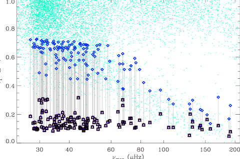
Figure 7: Observed visibilities $v_{1}$ for the Kepler public data set of red giants, as a function of $\nu_{\mathrm{max}}$. Values for stars showing depressed mixed modes are emphasized with large diamonds and compared to the computed visibilities: large dark triangles for the low-coupling case (Eq. (16), as in Unno et al., 1989; Fuller et al., 2015) are very close to black squares for the strong-coupling case (Eq. 20). Gray lines connect the observed and modelled values.

4 Observed versus predicted visibilities

As shown above, the observation of many red giants with depressed mixed modes invalidates the hypothesis of full suppression of the oscillation in the core for explaining low visibilities. This opens questions on the validity of Eq. (13) to explain the low visibility. Hence, we need to check whether the prediction of Eq. (13) is sustained. As our analysis is based on observations, we aim at checking Eq. (13) through Eq. (20). Therefore, we first justify the validity of using Eq. (20), then test various hypotheses introduced by Fuller et al. (2015) to explain low visibilities.

4.1 Global seismic parameters

Using Eq. (20) for testing the observed visibilities requires information on the coupling factors $q$ and on the radial mode widths $\Gamma_{0}$. The set of red giants with a low visibility and for which all parameters of Eq. (20) are measured is composed of $96$ stars. We assumed that the mechanism responsible for the extra damping does not modify the stellar interior structure, so that $q$ is representative of the transmission $T$. This assumption is theoretically justified by the analysis presented in Takata (2016b) and observationally verified: as seen above, all stars have similar $q$ and similar $\Gamma_{0}$, regardless the visibility (Figs. 3b and 3d). In that respect, the stars with depressed mixed modes provide us indirectly with relevant tests, and Eq. (20) can be used to test Eq. (13).

4.2 A significant disagreement

Assuming that $q$ measured from mixed modes can replace the $T$ value (Eq. 19) and using observed $\Gamma_{0}$, we could compare the relation between the reduced observed visibilities $v_{1}$ and the calculated depressed visibility $v$ predicted by Eq. (20). Contrary to previous work, the estimated visibilities do not match the observed visibilities, with modelled values significantly smaller than the observed values (Fig. 7). We stress that the discrepancy is not due to the use of the formalism correct for strong coupling introduced by Takata (2016a) and Takata (2016b). In fact, the difference is as high as a factor of 4 for the term $\tau_{0}\,T^{2}$ of Eq. (13). Relative uncertainties on $q$ and $\Gamma_{0}$ cannot explain such a high difference. We note however that the disagreement is consistent with partial suppression of the oscillation in the core since observed visibilities are larger than modelled values. This evidence is ascertained by the fact that, as made clear by Fig. 7, not only stars with depressed mixed modes have observed visibilities much larger than predicted by the model. The discrepancy certainly indicates that previous analysis were based on inappropriate estimates of $T$.

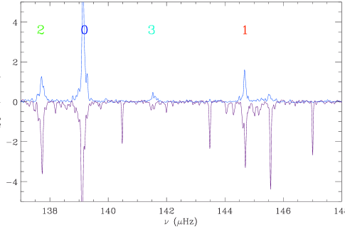
Figure 8: Comparison of the smoothed spectra of two stellar twins, KIC 5295898 (with depressed modes; blue curve) and KIC 2157650 (with normal modes, nearly seen pole on; purple curve printed upside down). The width of the smoothing filter is 0.05 $\mu$Hz, much smaller than the expected width of dipole modes if not mixed. A small shift in frequency is needed in order to superimpose the peaks.

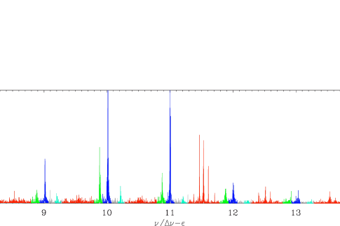
Figure 9: Spectrum of the RGB star KIC 6975038 showing a strong gradient of the dipole mode amplitudes. Dipole modes have very low amplitudes below the radial order 11 and normal amplitudes above.

5 Discussion

5.1 Depressed modes are mixed

Important facts were inferred from the observations presented in the previous sections: first, depressed modes are identified as mixed modes for all stars observed with a sufficient signal-to-noise ratio; second, period spacings of stars with depressed modes resemble normal period spacings; third, core rotation rates also follow the normal distribution. We next consider these three bits of information.

5.1.1 Depressed mixed modes

Mixed modes were directly or indirectly observed in many stars showing low visibilities. As already stated, the hypothesis of full suppression of the oscillation in the core is invalidated, since mixed modes result from the coupling of pressure waves in the envelope and gravity waves in the core. This observational result breaks the statement that the observation of low visibilities implies the suppression of the oscillation in the core. A mechanism able to only partially damp the oscillation is needed for explaining the low visibilities.

As a result, the mechanism proposed by Fuller et al. (2015) is not fully adequate since it relies on the total suppression of the dipole modes in the core. Furthermore, the equivalence between low visibility and magnetic greenhouse effect accepted in follow-up papers (Cantiello et al., 2016; Stello et al., 2016b) is questionable.

5.1.2 Period spacings of depressed mixed modes

The measurement of normal period spacings in stars with depressed modes allows us to derive further information, since such spacings imply that the resonant cavity of gravity modes is not perturbed by the suppression mechanism. The mechanism responsible for the damping cannot modify the Brunt-Väisälä cavity, at the high level of precision reached with seismology.

In that respect, the scattering process associated to the magnetic greenhouse effect is invalidated since it would modify the resonance condition of dipole modes, with a smaller resonant cavity for the gravity waves (Fig. 1 of Fuller et al., 2015), hence larger period spacings. Larger period spacings are not observed for depressed mixed modes. This proves that the magnetic greenhouse effect cannot explain the many cases where depressed mixed modes are observed. This mechanism may work in some other cases, but proving it then requires more information than simply the visibilities of dipole modes. In any case, at this stage, the magnetic greenhouse effect cannot be a general solution for explaining depressed modes, and it is impossible to conclude on the identity of the mechanism able to lower the dipole mode amplitude.

5.1.3 Rotational splittings of depressed mixed modes

The identification of the normal rotational splittings in stars with depressed modes provides us with similar conclusions.

If there were a strong magnetic field in the cores of the stars with depressed modes, then Cantiello et al. (2016) predict that an extra magnetic splitting, comparable to the gravity mode period spacing in RGB stars, would be observed. As the core rotation rates inferred from the mixed-mode pattern follow a similar distribution to the reference set of stars, we can rule out the presence of the extra, magnetic splitting.

5.2 From individual visibilities to extra damping

The study of the widths of dipole mixed modes can give promising information on the way amplitude are distributed in mixed modes. We illustrate this potential with the comparison of two twin stars with very close $\Delta\nu$ and $\Delta\Pi_{1}$. The star with normal visibility is used as a reference for the other with depressed modes. The resemblance of their mixed-mode pattern allowed us to compare their individual visibilities $v_{{n_{\mathrm{m}}}}$ (Fig. 8). The simplifications introduced either for normal stars (Section 2.2) or in the extreme case of full suppression of the oscillation in the core (Section 2.3) do not hold any more for the star with depressed modes. We have to rewrite Eq. (4) in case of an extra damping. For radial modes, we have

$$\Gamma_{0}I_{0}=-{1\over\omega_{0}}\oint\delta W_{0},$$ (23)

where $\omega_{0}$ is the radial frequency and the cyclic integral represents the work during one radial oscillation. For a mixed mode, we have an extra damping, so that

$$\Gamma_{n_{\mathrm{m}}}I_{n_{\mathrm{m}}}=-{1\over\omega_{n_{\mathrm{m}}}}\oint\delta W_{n_{\mathrm{m}}}\simeq-{1\over\omega_{n_{\mathrm{m}}}}\oint(\delta W_{0}+\delta W_{\mathrm{extra}}),$$ (24)

assuming that the normal dipole work is similar to the radial work, except for the extra damping (e.g., Dupret et al., 2009; Benomar et al., 2014; Grosjean et al., 2014). Since radial and non-radial frequencies are close to each other, we have

$$\Gamma_{n_{\mathrm{m}}}I_{n_{\mathrm{m}}}=\Gamma_{0}I_{0}\,(1+x),$$ (25)

with a similar definition for $x$ as in Eq. (10): $x$ represents the relative contribution of the extra damping.

From Eq. (4), we obtain a new expression for the mixed mode visibility,

$$v_{{n_{\mathrm{m}}}}\simeq{I_{0}\over(1+x)\,I_{n_{\mathrm{m}}}\ }\simeq{\Gamma_{n_{\mathrm{m}}}\over(1+x)^{2}\ \Gamma_{0}},$$ (26)

which demonstrates the capability of mixed modes to measure the relative extra damping $x$.

If we simply assume that $x$ has limited variation in frequency, the total contribution $v$ of the individual visibilities provides an estimate of the extra damping,

$$x\simeq{1-v\over v}.$$ (27)

According to this relation, the magnitude of this relative extra-damping significantly decreases with stellar evolution. Very low visibilities observed for stars on the low RGB are due to a large absorption ($x\simeq 9$ when $v_{1}=0.1$), but $x\simeq 0.7$ only when $v_{1}=0.6$. For KIC 5295898 shown in Fig. 8, $x\simeq 2.6$.

5.3 No man’s land

For completeness, we fitted the stars in the no man’s land between normal and low-visibility stars (Figs. 3a and 7). We checked that these stars behave as other stars, with similar seismic parameters. The presence of such stars is crucial for at least two reasons. First, they show that intermediate values between normal and low visibilities are possible. Second, those stars represent the intermediate case between normal and low visibility. This reinforces the fact that stars where depressed mixed modes could be fully characterized are representative of all stars with low-amplitude dipole modes.

5.4 Visibility gradient

Three stars of our data set exhibit a clear visibility gradient: KIC 6975038 (Fig. 9), 7746983, and 8561221.

- The case of KIC 6975038 is investigated in Mosser et al. (2016). This star shows atypical seismic parameters: $\Delta\Pi_{1}$ is very low and $q$ is unusually large compared to the general trend on the RGB (Mosser et al., 2015; Vrard et al., 2016). This star deserves a precise modelling beyond the scope of this work.

- KIC 8561221 was identified by García et al. (2014) as the least evolved observed star with depressed dipole modes among red giants observed with Kepler. It shows a very low dipole-mode visibility (Table 1). However, mixed modes can be firmly identified. The asymptotic period spacing $\Delta\Pi_{1}\simeq 114.8\,$s is typical for $\Delta\nu\simeq 29.8\,\mu$Hz, but the core rotation of this star seems very high. We measure a core rotation rate of about 2.6 $\mu$Hz, in contradiction with the values extracted from $\ell=2$ and $\ell=3$ modes by García et al. (2014).

- Compared to the two previous stars, the seismic parameters of KIC 7746983 are close to the values obtained on the RGB; only the dipole mode visibility is atypical. This gradient appears to be helpful for characterizing the mixed mode pattern: after KIC 8561221, this star is the second least evolved in our data set with low-dipole visibility.

The change of visibility with frequency was used by Fuller et al. (2015) as a further argument in favor of a large magnetic field for explaining the suppression of the oscillation, since the variation of the visibility with frequency matches their prediction. A more conservative analysis consists in remarking that the physics of oscillation damping has to be frequency dependent. Red giants showing a gradient of dipole visibility are certainly useful benchmark stars for understanding the nature and the physics of the extra damping of the oscillation.

6 Conclusion

We performed a thorough study of red giants showing low dipole-mode visibility, based on the identification of their dipole mode pattern and on the characterization of their global seismic properties. We have shown that these stars share the same global seismic parameters as other stars, regardless the value of the dipole mode visibilities. This analysis sustains the fact that the mechanism responsible for the damping does not significantly impact the stellar structure and does not change the property of the cavity where gravity waves propagate.

We were able to determine that dipole depressed modes are mixed, even at very low visibilities. The existence of these depressed mixed modes implies that oscillations cannot be fully suppressed in the radiative core. We also note that the observed visibilities are significantly higher than predicted from the modelling assuming full suppression in the core, which is consistent with partial suppression of the core oscillation only. Furthermore, the observations of normal period spacings in stars with depressed mixed modes indicates that the radiative core of these stars is not affected by the suppression mechanism.

These precise seismic signatures indicate that the magnetic greenhouse effect cannot explain the observed low visibilities of dipole modes (Fuller et al., 2015). This effect supposes the full suppression of the oscillation, which is discarded by the fact that depressed modes are mixed. Even if the mechanism could work with partial suppression only, the scattering process induced by the magnetic field in the radiative core is dismissed by the observation of the period spacings. As a result, inferring high magnetic fields in red giant from low visibilities (Stello et al., 2016b; Cantiello et al., 2016) is at least premature. This conclusion applies in the vast majority of stars that show low visibilities.

The low integrated visibilities reflect an extra mode damping but, at this stage, carry no direct information on the nature of this damping. Another damping mechanism must be found. This mechanism, which partially damps the dipole mixed modes, could be characterized by the measurement of the mixed mode widths.