A spacetime DPG method for the Schrödinger equation

Abstract.

A spacetime discontinuous Petrov-Galerkin (DPG) method for the linear time-dependent Schrödinger equation is proposed. The spacetime approach is particularly attractive for capturing irregular solutions. Motivated by the fact that some irregular Schrödinger solutions cannot be solutions of certain first order reformulations, the proposed spacetime method uses the second order Schrödinger operator. Two variational formulations are proved to be well posed: a strong formulation (with no relaxation of the original equation) and a weak formulation (also called the “ultraweak formulation”, which transfers all derivatives onto test functions). The convergence of the DPG method based on the ultraweak formulation is investigated using an interpolation operator. A stand-alone appendix analyzes the ultraweak formulation for general differential operators. Reports of numerical experiments motivated by pulse propagation in dispersive optical fibers are also included.

1. Introduction

This paper is devoted to exploring a weak formulation and an accompanying numerical technique for the Schrödinger equation with Dirichlet boundary conditions. Let $\varOmega_{0}\subset\mathbb{R}^{n}$ $(n\geq 1)$ be an open bounded domain with Lipschitz boundary. The space variable $x$ lies in $\varOmega_{0}$ while the time variable $t$ lies in the open interval $(0,T)$ with $T<\infty$. The classical form of Schrödinger initial boundary value problem reads as follows:

$$i\partial_{t}u-\Delta_{x}u =f, \quad x\in\varOmega_{0},\;0<t<T,$$ (1.1a)

$$u(x,t) =0, \quad x\in\partial\varOmega_{0},\;0<t<T,$$ (1.1b)

$$u(x,0) =0, \quad x\in\varOmega_{0},$$ (1.1c)

where $\partial_{t}$ denotes the time derivative $\partial/\partial t$ and $\Delta_{x}$ denotes the Laplacian with respect to the spatial variable $x$. Here $f$ is any given function in $L^{2}(\varOmega)$ and $\varOmega=\varOmega_{0}\times(0,T)$ throughout.

The numerical technique we want to apply to (1.1) is the discontinuous Petrov-Galerkin (DPG) method [14]. Among its desirable properties are mesh-independent stability, inheritance of discrete stability from the well-posedness of the undiscretized problem, and the availability of a canonical error indicator computed as part of the solution. The DPG method has been successfully applied to a wide variety of problems such as second order elliptic problems [11], convective phenomena [9, 10, 13], elasticity [2, 7, 21, 22], Stokes flow [7, 25], and spacetime problems [15, 16, 28]. It seems natural therefore that the DPG method should work for (1.1) as well. In this paper, we will show that the DPG method does indeed faithfully approximate the solutions of (1.1) provided we do not recast (1.1) into a first order system.

Many applications of interest come a first order systems even if they are often displayed as second order partial differential equations. For example, the second order heat equation is really a combination of two first order equations, namely the Fourier law of heat conduction and the conservation of energy. Similarly, the linear elasticity equation, while often displayed as a second order equation for displacement, is really a combination of two first order equations, the constitutive (Hooke’s) law and the equation of static equilibrium. Thus it’s no surprise that it makes physical sense to return the heat equation or the elasticity equation to first order form before discretizing. However, it makes no physical sense to do this for the Schrödinger equation, which is not derived from first order physical laws.

It makes no mathematical sense either. One might be tempted to introduce a “flux” $\tau,$ formulate the first order system $i\partial_{t}u-\mathrm{div}_{x}\tau=f$ and $\nabla_{x}u-\tau=g,$ and claim the latter’s equivalence to (1.1) when $g=0.$ This claim is false because, while the Schrödinger problem (1.1) is well-posed for $f\in L^{2}(\varOmega)$, the first order system cannot be well-posed in $L^{2}(\varOmega).$ Indeed, denoting the norm of $L^{2}(\varOmega)$ by $\|\cdot\|_{\varOmega}$, if the first order system were well-posed, then there would be constants $C_{1},C_{2}>0$ such that $\|u\|_{\varOmega}+\|\tau\|_{\varOmega}\leq C_{1}\|f\|_{\varOmega}+C_{2}\|g\|_{\varOmega}.$ But then the second equation of the system implies that $\|\nabla_{x}u\|_{\varOmega}=\|g+\tau\|_{\varOmega}\leq C_{1}\|f\|_{\varOmega}+2C_{2}\|g\|_{\varOmega}$ for any solution $u$, which is false: In the next two paragraphs we will exhibit a Schrödinger solution for which $\|\nabla_{x}u\|_{\varOmega}=\infty$ even when $g=0$ and $f\in L^{2}(\varOmega)$.

First observe that given any $f(x,t)$ in $L^{2}(\varOmega)$, it is possible to solve (1.1) by the “method of Galerkin approximations” [18] (distinct from the Galerkin finite element method). Let $e_{k}(x)$ in $H_{0}^{1}(\varOmega_{0})$ and $\omega_{k}^{2}>0$ be an eigenpair of $\Delta_{x}$ satisfying

$$-\Delta_{x}e_{k}=\omega_{k}^{2}e_{k}\qquad\text{ a.e. in }\varOmega_{0},$$ (1.2)

normalized so that $\|e_{k}\|_{\varOmega_{0}}=1$ for all natural numbers $k\geq 1$. Since Fubini’s theorem for product measures implies that $f(\cdot,t)$ is in $L^{2}(\varOmega_{0})$, the following definitions make sense:

$$f_{k}(t) =\int_{\varOmega_{0}}f(x,t)\bar{e}_{k}(x)\;dx, u_{k}(t) =-i\int_{0}^{t}e^{i\omega_{k}^{2}(t-s)}f_{k}(s)\;ds,$$ (1.3a)

$$F_{M}(x,t) =\sum_{k=1}^{M}f_{k}(t)e_{k}(x), U_{M}(x,t) =\sum_{k=1}^{M}u_{k}(t)e_{k}(x).$$ (1.3b)

It is not difficult to show (see the proof of Theorem 2.4 below) that $u=\lim_{M\to\infty}U_{M}$ exists in $L^{2}(\varOmega)$ and solves (1.1).

Now consider the one-dimensional case $\varOmega_{0}=(0,1)$, where $\omega_{k}=k\pi$, and choose

$$f(x,t)=\sum_{k=1}^{\infty}\frac{1}{k}e^{i\omega_{k}^{2}t}e_{k}(x)\quad\text{ in }L^{2}(\varOmega).$$

Then by the orthonormality of $e_{k}$, we have that $f_{k}(s)=e^{i\omega_{k}^{2}s}/k$, $u_{k}(t)=-ite^{i\omega_{k}^{2}t}/k$,

$$\|U_{M}\|_{\varOmega}^{2} =\sum_{k=1}^{M}\int_{0}^{T}|u_{k}(t)|^{2}\,dt=\sum_{k=1}^{M}\int_{0}^{T}\left|\frac{-it}{k}e^{i\omega_{k}^{2}t}\right|^{2}dt=\frac{T^{3}}{3}\sum_{k=1}^{M}\frac{1}{k^{2}},$$

$$\|\nabla_{x}U_{M}\|^{2}_{\varOmega} =\sum_{k=1}^{M}\omega_{k}^{2}\int_{0}^{T}\left|u_{k}(t)\right|^{2}\,dt=T^{3}\sum_{k=1}^{M}\frac{\omega_{k}^{2}}{3k^{2}}=\frac{\pi^{2}}{3}T^{3}M.$$

The solution $u$ is the limit of $U_{M}$. The above calculations clearly show that as $M\to\infty$, while $\|u\|_{\varOmega}=\lim_{M\to\infty}\|U_{M}\|_{\varOmega}=(T^{3}\pi^{2}/18)^{\frac{1}{2}}$, the limit of $\|\nabla_{x}U_{M}\|_{\varOmega}$ diverges. Thus it is possible to obtain a Schrödinger solution $u$ whose $H^{1}$-norm is infinite even when $f\in L^{2}(\varOmega)$. Note that finer arguments are needed to understand the regularity of Schrödinger solutions in unbounded domains, which although a topic of wide mathematical interest [27], is not our concern here.

To our knowledge, this paper is the first work to analyze the feasibility of the DPG methodology for a system without ready access to an equivalent first order formulation. The second order form necessitates formulations in the nonstandard graph spaces of the second order Schrödinger operator. One of the contributions of this paper is the proof of well-posedness of a strong and a weak formulation of (1.1) in these graph spaces. The general spaces and arguments required for this analysis are collected in a stand-alone appendix (Appendix A), anticipating uses outside of the Schrödinger example. The analysis in Appendix A is motivated by the modern theory of Friedrichs systems [17] but applies beyond Friedrichs systems. Borrowing the approach of [17], we are able to prove well-posedness without developing a trace theory for the graph spaces. The other contributions involve the numerical implications of this well-posedness. Numerical methods using the strong formulation must use conforming finite element subspaces of the graph spaces. On the other hand, numerical methods using the weak formulation need only use existing standard finite element spaces. In either case, an interpolation theory in the Schrödinger graph norm is needed to estimate convergence rates. We address this issue in one space dimension.

In the next section, we investigate well-posedness (in the sense of Hadamard) for a strong and weak variational formulation for the Schrödinger problem. This will require an abstract definition of a boundary operator and duality pairings in a graph space. Such abstract definitions that apply beyond the Schrödinger setting are in Appendix A. Their particular realizations for the Schrödinger case are used in section 2. (To avoid repetitions of the general definitions in the specific case, we will often refer to Appendix A in section 2.) Section 3 provides a verification of a density assumption made in section 2. Section 4 details our construction of a conforming finite element space and interpolation error estimates. Section 5 points to an application in dispersive optical fibers and contains some numerical results.

2. Functional Setting and Wellposedness

We now provide a functional setting within which a strong and a weak formulation of the spacetime Schrödinger problem can be proved to be well posed (i.e., inf-sup stable). The analysis is an application of the general theory detailed in Appendix A.

The classical form of the problem is already presented in (1.1). Recalling that $\varOmega=\varOmega_{0}\times(0,T)$, define these parts of $\partial\varOmega$:

$$\varGamma=\partial\varOmega_{0}\times[0,T]\cup\varOmega_{0}\times\{0\},\qquad\varGamma^{*}=\partial\varOmega_{0}\times[0,T]\cup\varOmega_{0}\times\{T\}$$

(see Figure 1). Then the initial and boundary conditions together can be written as $u|_{\varGamma}=0$. We want to write (1.1) as an operator equation (see (A.8)) to apply the general results of Appendix A. To this end, consider the setting of Appendix A with

$$A=A^{*}=i\partial_{t}-\Delta_{x},\qquad k=l=m=1,\;d=n+1.$$

The space $W=W^{*}$ is then defined by (A.2)–(A.3); namely, $W=W^{*}=\{u\in L^{2}(\varOmega):\;i\partial_{t}u-\Delta_{x}u\in L^{2}(\varOmega)\}$. The operator $D=D^{*}:W\to W^{\prime}$ is defined by (A.5)–(A.6); namely, $\langle{Dw,\tilde{w}}\rangle_{W}=(Aw,\tilde{w})_{\varOmega}-(w,A\tilde{w})_{\varOmega}$ for all $w,\tilde{w}\in W.$ As usual, let $\mathcal{D}(\bar{\varOmega})$ denote the restrictions of functions from $\mathcal{D}(\mathbb{R}^{n+1})$ to $\varOmega$. The operator $D$ (often called the “boundary operator” in the theory of Friedrichs systems [17]), satisfies

$$\langle{D\phi,\psi}\rangle_{W}=\int_{\partial\varOmega}in_{t}\phi\bar{\psi}+\int_{\partial\varOmega}\phi(n_{x}\cdot\nabla_{x}\bar{\psi})-\int_{\partial\varOmega}(n_{x}\cdot\nabla_{x}\phi)\bar{\psi}$$ (2.1)

for all $\phi,\psi\in\mathcal{D}(\bar{\varOmega})$. Note that although the integrals on the right-hand side need not exist for all functions in $W$, $D$ is defined on all $W$ through (A.5).

Although we set the differential operators $A$ and $A^{*}$ to be equal above, note that we consider each as an unbounded operator with its own domain. We set the domain of $A$ to

$$\mathop{\mathrm{dom}}(A)=\{u\in W:\langle Dv,u\rangle_{W}=0,\,\forall v\in\mathcal{V}^{*}\},$$ (2.2)

where $\mathcal{V}^{*}=\{\varphi\in\mathcal{D}(\bar{\varOmega}):\;\varphi|_{\varGamma^{*}}=0\}.$ The domain of the adjoint is given by the usual [3, 24] general prescription: $\mathop{\mathrm{dom}}(A^{*})=\{s\in L^{2}(\varOmega)^{l}:$ $\exists\,\ell\in L^{2}(\varOmega)^{m}$ such that $(Av,s)_{\varOmega}=(v,\ell)_{\varOmega}$ $\forall v\in\mathop{\mathrm{dom}}(A)\}.$ Here $(\cdot,\cdot)_{\varOmega}$ denotes the (complex) inner product in $L^{2}(\varOmega)$. Finally, as in the appendix, set $V=\mathop{\mathrm{dom}}(A)$ and $V^{*}=\mathop{\mathrm{dom}}(A^{*})$ with the understanding that both $V$ and $V^{*}$ are endowed with the $W$-topology, while $\mathop{\mathrm{dom}}(A)$ and $\mathop{\mathrm{dom}}(A^{*})$ have the topology of $L^{2}(\varOmega)$.

Figure 1. Schematic of the spacetime domain

For the above set $A,A^{*}$ and $\mathop{\mathrm{dom}}(A)$, the conditions (A-a) and (A-b) in Appendix A are immediate, while condition (A-c) is easily verified using (2.1). Hence Lemma A.2 shows that $\mathop{\mathrm{dom}}(A^{*})$ equals

$$V^{*}=\sideset{{}^{\perp}}{}{\mathop{D(V)}}.$$ (2.3)

Rewriting (2.2) in the same style,

$$V=\sideset{{}^{\perp}}{}{\mathop{D(\mathcal{V}^{*})}}.$$ (2.4)

Thus $V$ and $V^{*}$ are closed subspaces of $W$. Let $\mathcal{V}=\{\varphi\in\mathcal{D}(\bar{\varOmega}):\;\varphi|_{\varGamma}=0\}$.

Lemma 2.1.

$\mathcal{V}\subset V$ and $\mathcal{V}^{*}\subset V^{*}$.

Proof.

Equation (2.1) implies $\langle{D\phi,\phi^{*}}\rangle_{W}=0$ for all $\phi\in V$ and $\phi^{*}\in\mathcal{V}^{*}.$ Hence, any $\phi\in\mathcal{V}$ is also in $\sideset{{}^{\perp}}{}{\mathop{D(\mathcal{V}^{*})}},$ which by (2.4) implies that $\phi\in V$. Thus $\mathcal{V}\subset V$.

If $\phi^{*}\in\mathcal{V}^{*}$, then (2.2) shows that $\langle{D\phi^{*},u}\rangle_{W}=0$ for all $u\in V$, i.e., $\phi^{*}\in\sideset{{}^{\perp}}{}{\mathop{D(V)}},$ which by (2.3) implies $\phi^{*}$ is in $V^{*}$. ∎

In (2.4), $\mathcal{V}^{*}$ may be replaced by $V^{*},$ provided that a density result is available, as we show next.

Assumption 1.

Suppose that $\mathcal{V}^{*}$ is dense in $V^{*}$ and that $\mathcal{V}$ is dense in $V$.

Lemma 2.2.

If Assumption 1 holds, then $\sideset{{}^{\perp}}{}{\mathop{D(\mathcal{V}^{*})}}=\sideset{{}^{\perp}}{}{\mathop{D(V^{*})}}$ and $\sideset{{}^{\perp}}{}{\mathop{D(\mathcal{V})}}=\sideset{{}^{\perp}}{}{\mathop{D(V)}}.$

Proof.

Clearly $\mathcal{V}^{*}\subseteq V^{*}$ implies $\sideset{{}^{\perp}}{}{\mathop{D(\mathcal{V}^{*})}}\supseteq\sideset{{}^{\perp}}{}{\mathop{D(V^{*})}}.$ To prove the reverse containment, suppose $w\in\sideset{{}^{\perp}}{}{\mathop{D(\mathcal{V}^{*})}}$ and $v^{*}\in V^{*}$. By density, there is a sequence $\tilde{v}_{n}$ in $\mathcal{V}^{*}$ satisfying $\lim_{n\to\infty}\|\tilde{v}_{n}-v^{*}\|_{W}=0$. Since $\langle{D\tilde{v}_{n},w}\rangle_{W}=0,$ by the continuity of $D$, we have $\langle{Dv^{*},w}\rangle_{W}=0.$ Hence $w\in\sideset{{}^{\perp}}{}{\mathop{D(V^{*})}}$. The second identity is proved similarly. ∎

2.1. Strong formulation

The strong formulation of the Schrödinger problem (1.1) is based on these sesquilinear and conjugate linear forms:

$$a(u,v)=(Au,v)_{\varOmega},\qquad l(v)=(f,v)_{\varOmega}.$$

Problem 2.3 (Strong formulation).

Given any $f\in L^{2}(\varOmega)$, find $u\in V$ satisfying

$$a(u,v)=l(v),\qquad\,\forall v\in L^{2}(\varOmega).$$

Theorem 2.4.

Suppose that Assumption 1 holds. Then the linear Schrödinger operator $A:V\rightarrow L^{2}(\varOmega)$ is a continuous bijection. Hence Problem 2.3 is well-posed.

Proof.

To prove the surjectivity of $A$, suppose $f\in L^{2}(\varOmega)$. Recall the definitions of $e_{k}$, $u_{k}$ and $f_{k}$ from (1.2) and (1.3). Clearly, $AU_{M}=F_{M}$. Since $U_{M}$ and any $\varphi\in\mathcal{V}^{*}$ are smooth enough for integration by parts using $\varphi|_{\varGamma^{*}}=0$ and $U_{M}|_{\varGamma}=0,$ we have

$$(i\partial_{t}U_{M},\varphi)_{\varOmega} =(U_{M},i\partial_{t}\varphi)_{\varOmega},$$

$$(\Delta U_{M},\varphi)_{\varOmega} =(U_{M},\Delta\varphi)_{\varOmega}.$$

Hence $\langle{D\varphi,U_{M}}\rangle_{W}=(A\varphi,U_{M})_{\varOmega}-(\varphi,AU_{M})_{\varOmega}=0$ for all $\varphi\in\mathcal{V}^{*}.$ By (2.4), this implies that $U_{M}$ is in $V$.

Next, we show that $U_{M}$ is a Cauchy sequence in $V$. For any $N>M$,

$$\|U_{M}-U_{N}\|_{\varOmega}^{2} =\sum_{k=M+1}^{N}\int_{0}^{T}|u_{k}(t)|^{2}\;dt\leq\frac{1}{2}T^{2}\sum_{k=M+1}^{\infty}\int_{0}^{T}|f_{k}(t)|^{2}\;dt,$$

$$\|A(U_{M}-U_{N})\|_{\varOmega}^{2} =\|F_{M}-F_{N}\|_{\varOmega}^{2}\leq\sum_{k=M+1}^{\infty}\int_{0}^{T}|f_{k}(t)|^{2}\;dt,$$

both of which converge to 0 as $M\to\infty$, because $f\in L^{2}(\varOmega)$. Thus $U_{M}$ is Cauchy. It must therefore have an accumulation point $u$ in $V$. Moreover, since $Au$ and $f$ are $L^{2}(\varOmega)$-limits of the same sequence $F_{M}=AU_{M}$, we have $Au=f$. Thus $A:V\to L^{2}(\varOmega)$ is surjective.

We use a similar argument (with $u_{k}$ defined by integrals from $T$ to $t$) to show that $A=A^{*}:V^{*}\to L^{2}(\varOmega)$ is also surjective. We omit the details, but note that the only difference is that instead of (2.4), we must now use

$$V^{*}=\sideset{{}^{\perp}}{}{\mathop{D(\mathcal{V})}},$$

which follows from (2.3), Assumption 1 and Lemma 2.2. Finally, since $\ker(A)={{\sideset{{}^{\perp}}{}{\mathop{\mathop{\mathrm{ran}}(A^{*})}}}}$, the surjectivity of $A^{*}:V^{*}\to L^{2}(\varOmega)$ shows that $A:V\to L^{2}(\varOmega)$ is injective, thus completing the proof of the stated bijectivity. ∎

Remark 2.5.

An example of a standard well-posedness result for the Schrödinger equation obtained using semigroup theory is [23, Theorem 4.8.1], which proves that there is one and only one solution to (1.1) whenever $f\equiv 0$ and $u(x,0)$ is in $H^{2}(\varOmega)\cap H_{0}^{1}(\varOmega)$. In Theorem 2.4, we have shown (by a different method) that the existence of a unique solution holds for any $f\in L^{2}(\varOmega)$. Note that in the above proof, we used Assumption 1 only to obtain injectivity. If one opts to use the results of [23] (with $u(x,0)\equiv 0$ and $f\equiv 0$) to conclude injectivity, then there is no need to place Assumption 1 in Theorem 2.4.

2.2. A weak formulation

Now we consider a mesh-dependent weak formulation that is the basis of the DPG method. This formulation, sometimes called the “ultraweak” formulation, is given in a general setting in Problem A.4 of Appendix A. We apply this to our example of the Schrödinger equation.

The spacetime domain $\varOmega$ is partitioned into a mesh $\varOmega_{h}$ of finitely many open elements $K$ such that $\bar{\varOmega}=\cup_{K\in\varOmega_{h}}\bar{K}$ where $h=\max_{K\in\varOmega_{h}}\mathop{\mathrm{diam}}(K)$. Particularizing the general definitions in Appendix A (see (A.9) through (A.11)) to the Schrödinger example, we let $A_{h}=A_{h}^{*}$ be the Schrödinger operator applied element by element and let $W_{h}=W_{h}^{*}=\{w\in L^{2}(\varOmega):A(w|_{K})\in L^{2}(K)$ for all $K\in\varOmega_{h}\}$. The operator $D_{h}:W_{h}\to W_{h}^{\prime}$ is defined by $\langle{D_{h}w,v}\rangle_{W_{h}}=(A_{h}w,v)_{\varOmega}-(w,A_{h}v)_{\varOmega}$ for all $w,v\in W_{h}$ and let $D_{h,V}:V\to W_{h}^{\prime}$ be denote $D_{h}|_{V}$. The range of $D_{h,V}$, denoted by $Q,$ is made into a complete space by the norm $\|q\|_{Q}=\inf_{v\in D_{h,V}^{-1}(\{q\})}\|v\|_{W}$. Abbreviating the duality pairing $\langle{\cdot,\cdot}\rangle_{W_{h}}$ by $\langle{\cdot,\cdot}\rangle_{h}$, define the sesquilinear form $b((u,q),v)=(u,A_{h}v)_{\varOmega}+\langle{q,v}\rangle_{h}$ on $(L^{2}(\varOmega)\times Q)\times W_{h}$.

Problem 2.6 (Ultraweak formulation).

Given $F\in W_{h}^{\prime},$  find $u\in L^{2}(\varOmega)$ and $q\in Q$ such that

$$b((u,q),v)=F(v)\qquad\forall v\in W_{h}.$$

Theorem 2.7.

Suppose that Assumption 1 holds. Then Problem 2.6 is well-posed, i.e., there is a $C>0$ such that given any $F\in W_{h}^{\prime}$, there is a unique solution $(u,q)\in L^{2}(\varOmega)\times Q$ to Problem 2.6 that satisfies

$$\|u\|_{\varOmega}^{2}+\|q\|_{Q}^{2}\;\leq\,C\,\|F\|_{W_{h}^{\prime}}^{2}.$$

Moreover, if $F(v)=(f,v)_{\varOmega}$ for some $f\in L^{2}(\varOmega),$ then $u$ is in $V$ and $q=D_{h}u$.

Proof.

The result follows from Theorem A.5. Since Lemma 2.2 together with (2.4) implies (A.12) and since Theorem 2.4 implies (A.13), the assumptions of Theorem A.5 are verified. ∎

3. Verification of the density assumption

In the next three sections, $\varOmega_{0}$ is set to be the interval $(0,L)$ and $\varOmega=(0,L)\times(0,T)$ where $L,T>0.$ The purpose of this section is to verify the density assumption (Assumption 1) in this case of one space dimension.

Theorem 3.1.

Let $\varOmega=(0,L)\times(0,T)$. Then $\mathcal{V}^{*}=\{\varphi\in\mathcal{D}(\bar{\varOmega}):\varphi|_{\varGamma^{*}}=0\}$ is dense in $V^{*}$, and $\mathcal{V}=\{\varphi\in\mathcal{D}(\bar{\varOmega}):\varphi|_{\varGamma}=0\}$ is dense in $V.$

Proof.

Since the proofs of both the stated density results are similar, we will only show the proof of density of $\mathcal{V}^{*}$ in $V^{*}$.

Step 1. Extend: Let $\varOmega_{l}=(-L,0]\times(0,T)$ and $\varOmega_{r}=[L,2L)\times(0,T)$. Define an operator $G$ that extends functions on $\varOmega$ to $\hat{\varOmega}\equiv\varOmega_{l}\cup\varOmega\cup\varOmega_{r}$ by

$$Gw(x,t)=\left\{\begin{aligned} -&w(-x,t),&&\;(x,t)\in\varOmega_{l},\\ -&w(2L-x,t),&&\;(x,t)\in\varOmega_{r},\end{aligned}\right.$$

(and $Gw(x,t)=w(x,t)$ for all $(x,t)\in\varOmega$). Let $G^{\prime}$ be the reverse operator that maps functions on $\hat{\varOmega}$ to $\varOmega$ by $G^{\prime}\bar{w}(x,t)=\bar{w}(x,t)-\bar{w}(-x,t)-\bar{w}(2L-x,t)$ for all $(x,t)\in\varOmega$ (see Figure 2). Such definitions are to be interpreted a.e., so that, for example, $Gw$ is well defined for any $w$ in $L^{2}(\varOmega)$. It is easy to see by a change of variable that

$$(Gf,g)_{\hat{\varOmega}}=(f,G^{\prime}g)_{\varOmega},\qquad\forall f\in L^{2}(\varOmega),\;g\in L^{2}(\hat{\varOmega}).$$ (3.1)

Next, we claim that

$$AGv=GAv,\qquad\forall v\in V^{*}.$$ (3.2)

Clearly, $Gv$ is in $L^{2}(\hat{\varOmega})$. Let $\varphi\in\mathcal{D}(\hat{\varOmega})$. Let $\langle{AGv,\varphi}\rangle_{\mathcal{D}(\hat{\varOmega})}$ denote the action of the distribution $AGv$ on $\bar{\varphi}$. Then $\langle{AGv,\varphi}\rangle_{\mathcal{D}(\hat{\varOmega})}=(Gv,A\varphi)_{\hat{\varOmega}}=(v,G^{\prime}A\varphi)_{\varOmega}$ because of (3.1). By the chain rule applied to the smooth function $\varphi$, we find that

$$G^{\prime}A\varphi=AG^{\prime}\varphi.$$ (3.3)

Hence,

$$\langle{AGv,\varphi}\rangle_{\mathcal{D}(\hat{\varOmega})} =(v,AG^{\prime}\varphi)_{\varOmega}=(Av,G^{\prime}\varphi)_{\varOmega}-\langle{Dv,G^{\prime}\varphi}\rangle_{W}.$$ (3.4)

Now observe that $G^{\prime}\varphi|_{\varGamma}=0$. Hence, by Lemma 2.1, $G^{\prime}\varphi$ is in $V$. Since $v\in V^{*}$ and $G^{\prime}\varphi\in V$, the last term of (3.4) must vanish by (2.3). Thus $\langle{AGv,\varphi}\rangle_{\mathcal{D}(\hat{\varOmega})}=(Av,G^{\prime}\varphi)_{\varOmega}=(GAv,\varphi)_{\hat{\varOmega}},$ completing the proof of the claim (3.2). In view of (3.2), we conclude that $Gv$ is in $W(\hat{\varOmega})$ whenever $v\in V{{{}^{*}}}$.

Figure 2. Extension and translation in the proof of Theorem 3.1.

Step 2. Translate: Let $\tilde{G}v$ denote the extension of $Gv$ by zero to $\mathbb{R}^{2}$; i.e., $\tilde{G}v$ equals $Gv$ on $\hat{\varOmega}$ and equals zero elsewhere. Let $\tau_{\delta}$ be the translation operator in the $-t$ direction by $\delta$; i.e., $(\tau_{\delta}w)(x,t)=w(x,t+\delta).$ Its well known [3] that

$$\lim_{\delta\to 0}\|\tau_{\delta}g-g\|_{\mathbb{R}^{2}}=0\qquad\forall g\in L^{2}(\mathbb{R}^{2}).$$ (3.5)

Let $\hat{\varOmega}_{\delta}=(-L,2L)\times(-\delta,T+\delta)$ and let $H_{\delta}$ denote the restriction of functions on $\mathbb{R}^{2}$ to $\hat{\varOmega}_{\delta}$. By a change of variable,

$$(\tau_{\delta}\tilde{G}f,g)_{\hat{\varOmega}_{\delta}}=(Gf,\tau_{-\delta}g)_{\hat{\varOmega}}\qquad\forall f\in L^{2}(\varOmega),\;g\in L^{2}(\hat{\varOmega}_{\delta}).$$ (3.6)

We now claim that

$$AH_{\delta}\tau_{\delta}\tilde{G}v=H_{\delta}\tau_{\delta}\tilde{G}Av\qquad\forall v\in V^{*}.$$ (3.7)

Indeed, for any $\varphi\in\mathcal{D}(\hat{\varOmega}_{\delta})$, the action of the distribution $AH_{\delta}\tau_{\delta}\tilde{G}v$ on $\bar{\varphi}$ equals

$$\langle{AH_{\delta}\tau_{\delta}\tilde{G}v,\varphi}\rangle_{\mathcal{D}(\hat{\varOmega}_{\delta})} =(\tau_{\delta}\tilde{G}v,A\varphi)_{\hat{\varOmega}_{\delta}}=(Gv,A\tau_{-\delta}\varphi)_{\hat{\varOmega}}=(v,G^{\prime}A\tau_{-\delta}\varphi)_{\varOmega}=(v,AG^{\prime}\tau_{-\delta}\varphi)_{\varOmega}$$

$$=(Av,G^{\prime}\tau_{-\delta}\varphi)_{\varOmega}-\langle{Dv,G^{\prime}\tau_{-\delta}\varphi}\rangle_{W},$$

where we have used (3.6), (3.1), and (3.3) consecutively. Since $(G^{\prime}\tau_{-\delta}\varphi)|_{\varGamma}=0,$ Lemma 2.1 shows that $G^{\prime}\tau_{-\delta}\varphi$ is in $V$, and consequently the last term above vanishes for all $v\in V^{*}$. Continuing and using (3.1) and (3.6) once more, $\langle{AH_{\delta}\tau_{\delta}\tilde{G}v,\varphi}\rangle_{\mathcal{D}(\hat{\varOmega}_{\delta})}=(GAv,\tau_{-\delta}\varphi)_{\hat{\varOmega}}=(\tau_{\delta}\tilde{G}Av,\varphi)_{\hat{\varOmega}_{\delta}}.$ This proves (3.7).

Step 3. Mollify: Consider the mollifier $\rho_{\varepsilon}\in\mathcal{D}(\mathbb{R}^{2})$, for each $\varepsilon>0$, defined by $\rho_{\varepsilon}(x,t)=\varepsilon^{-2}\rho_{1}(\varepsilon^{-1}x,\varepsilon^{-1}t),$ where

$$\rho_{1}(x,t)=\left\{\begin{aligned} &k\,e^{-\frac{1}{1-x^{2}-t^{2}}}&&\text{ if }x^{2}+t^{2}<1,\\ &0&&\text{ if }x^{2}+t^{2}\geq 1,\end{aligned}\right.$$

and $k$ is a constant chosen so that $\int_{\mathbb{R}^{2}}\rho_{1}=1.$ It is well known [3] that when any function $w$ in $L^{2}(\mathbb{R}^{2})$ is convolved with $\rho_{\varepsilon}$, the result $\rho_{\varepsilon}*w$ is infinitely smooth and satisfies

$$\lim_{\varepsilon\to 0}\|w-\rho_{\varepsilon}*w\|_{\mathbb{R}^{2}}=0\qquad\forall\,w\in L^{2}(\mathbb{R}^{2}).$$ (3.8)

Consider any small enough $\delta>0$, say $\delta<\min(L/2,T/2)$, and define two functions $v_{\varepsilon}=\rho_{\varepsilon}*\tau_{\delta}\tilde{G}v$ and $a_{\varepsilon}=\rho_{\varepsilon}*\tau_{\delta}\tilde{G}Av.$ Note that the two smooth functions $Av_{\varepsilon}$ and $a_{\varepsilon}$ need not coincide everywhere. However, because of (3.7), they coincide on $\varOmega$ whenever $\varepsilon<\delta/2$:

$$Av_{\varepsilon}=a_{\varepsilon}\qquad\text{ on }\varOmega.$$

Let us therefore set $\delta$ to, say, $\delta=3\varepsilon$ and let $\varepsilon<\min(L/2,T/2)/3$ go to zero. Note that

$$\|Av_{\varepsilon}-Av\|_{\varOmega} =\|a_{\varepsilon}-Av\|_{\varOmega}=\|\rho_{\varepsilon}*\tau_{\delta}\tilde{G}Av-Av\|_{\varOmega}$$

$$\leq\|\rho_{\varepsilon}*\tau_{\delta}\tilde{G}Av-\tau_{\delta}\tilde{G}Av\|_{\mathbb{R}^{2}}+\|\tau_{\delta}\tilde{G}Av-\tilde{G}Av\|_{\mathbb{R}^{2}},$$

$$\|v_{\varepsilon}-v\|_{\varOmega} \leq\|\rho_{\varepsilon}*\tau_{\delta}\tilde{G}v-\tau_{\delta}\tilde{G}v\|_{\varOmega}+\|\tau_{\delta}\tilde{G}v-v\|_{\varOmega}$$

$$\leq\|\rho_{\varepsilon}*\tau_{\delta}\tilde{G}v-\tau_{\delta}\tilde{G}v\|_{\mathbb{R}^{2}}+\|\tau_{\delta}\tilde{G}v-\tilde{G}v\|_{\mathbb{R}^{2}}.$$

Using (3.8) and (3.5), it now immediately follows that

$$\lim_{\varepsilon\to 0}\|v_{\varepsilon}-v\|_{W}=0.$$

To conclude, examine the value of $v_{\varepsilon}$ at points $z=(0,t)$ for any $0<t<T$, namely

$$v_{\varepsilon}(0,t)=\int_{\mathbb{R}}\int_{\mathbb{R}}\rho_{\varepsilon}(-x^{\prime},t-t^{\prime})\;(\tau_{\delta}\tilde{G}v)(x^{\prime},t^{\prime})\;dx^{\prime}\,dt^{\prime}.$$

The integrand of the inner integral is the product of an even function $(\rho_{\varepsilon})$ of $x^{\prime}$ and an odd function $\tau_{\delta}\tilde{G}v$ of $x^{\prime}$. Hence $v_{\varepsilon}(0,t)=0$. The same holds for points $z=(L,t)$. Moreover, since $\tau_{\delta}\tilde{G}v(y)$ is identically zero in a neighborhood of $z=(T,x)$ for all $0<x<L$, we conclude that $v_{\varepsilon}|_{\varGamma^{*}}=0.$ ∎

4. Error Estimates for the ideal DPG method

Continuing to consider the set $\varOmega$ as defined in Section 3, we now proceed to analyze the convergence of the ideal DPG method for Problem 2.6. The ideal DPG method finds $u_{h}$ and $q_{h}$ in finite-dimensional subspaces $U_{h}\subset L^{2}(\varOmega)$ and $Q_{h}\subset Q$, respectively, satisfying

$$b((u_{h},q_{h}),v)=F(v)\qquad\forall v\in T(U_{h}\times Q_{h}).$$ (4.1)

Here $T:L^{2}(\varOmega)\times Q\to W_{h}$ is defined by $(T(z,r),v)=b((z,r),v)$ for all $v\in W_{h}$ and any $(z,r)\in L^{2}(\varOmega)\times Q$. The main feature of the ideal DPG method is that the well-posedness of Problem 2.6 implies quasioptimality of the method’s error [14]. The wellposedness of Problem 2.6 follows from Theorem 2.7, now that we have verified Assumption 1 in Theorem 3.1. Hence to obtain convergence rates for specific subspaces, we need only develop interpolation error estimates. Since the interpolation properties of the $L^{2}$-conforming $U_{h}$ are standard, we need only discuss those of $Q_{h}.$ To study this, we will create a spacetime finite element space $V_{h}\subset V$, then identify $Q_{h}$ as $D_{h}(V_{h})$, and finally establish interpolation estimates for $Q_{h}$ using those for $V_{h}$. Note that $V_{h}$ will be used only in the proof (and not in the computations).

To transparently present the ideas, we shall limit ourselves to the very simple case of a uniform mesh $\varOmega_{h}$ of spacetime square elements of side length $h$. Let $\mathcal{E}_{h}$ denote the set of edges of $\varOmega_{h}$. On any $E\in\mathcal{E}_{h},$ let $P_{p}(E)$ denote the space of polynomials on the edge of degree at most $p$. On any $K\in\varOmega_{h}$, let $Q_{p}(K)$ denote the space of polynomials of degree at most $p$ in $x$ and at most $p$ in $t$. To begin the finite element construction, we consider the reference element $\hat{K}=(0,1)\times(0,1)$ and the element space $Q_{p}(\hat{K}),$ endowed with the following degrees of freedom: For any $w\in H^{3}(K)$, and for each $i\in\{0,1,\dots,p-2\}$ and $j\in\{0,1,2,\dots,p\},$ write $x_{i}=i/(p-2)$ and $t_{j}=j/p$ and set

$$\sigma_{ij}(w)=w(x_{i},t_{j}),\qquad\sigma_{j}^{0}(w)=\partial_{x}w(0,t_{j}),\qquad\sigma_{j}^{1}(w)=\partial_{x}w(1,t_{j}).$$

Together, these form a set $\varSigma$ with $(p-1)(p+1)+2(p+1)$ linear functionals (see Figure 3). The triple $(\hat{K},Q_{k}(\hat{K}),\varSigma)$ is a unisolvent finite element, in the sense of [8], as we show next.

Figure 3. Degrees of freedom in the $p=3$ (left) and $p=5$ (right) cases.

Lemma 4.1.

Suppose $p\geq 3$. Then any polynomial $w\in Q_{p}(\hat{K})$ is uniquely defined by the values of its degrees of freedom $\sigma$ in $\varSigma.$

Proof.

Suppose $w\in Q_{p}(\hat{K})$ and $\sigma(w)=0$ for all $\sigma\in\varSigma$. Then $w_{j}(x)=w(x,t_{j})$ is a polynomial of degree $p$ in one variable ($x$). The Hermite and Lagrange degrees of freedom on $t=t_{j}$ imply $w_{j}=0$. Now, fixing $x$, observe that the polynomial $w(x,t)$ is of degree at most $p$ in the variable $t$ and has $p+1$ zeros. Hence $w\equiv 0$ and the proof is complete since $\dim Q_{p}(\hat{K})$ equals the number of degrees of freedom. ∎

Next, consider the global finite element space $W_{h}^{p}(\varOmega)=\{w\in L^{2}(\varOmega):\;\partial_{t}w$ and $\partial_{xx}w$ are in $L^{2}(\varOmega)$ and $w|_{K}\in Q_{p}(K)$ for all $K\in\varOmega_{h}\}.$ Each element $K\in\varOmega_{h}$ is obtained by mapping the reference element $\hat{K}$ by $T_{K}:\hat{K}\to K,$ $T_{K}(\hat{x},\hat{t})=(h\hat{x}+x_{K},h\hat{t}+t_{K})$, where $(x_{K},t_{K})$ is the lower left corner vertex of $K,$ and the element space $Q_{p}(K)$ is the pull back of the reference element space $Q_{p}(\hat{K})$ under this map. The space $W_{h}^{p}(\varOmega)$ can be controlled by a global set of degrees of freedom obtained by mapping the reference element degrees of freedom and, as usual, coalescing those that coincide at the mesh element interfaces.

On the reference element $\hat{K}$, the degrees of freedom define an interpolation operator

$$\hat{\varPi}w=\sum_{\sigma\in\varSigma}\,\sigma(w)\,\varphi_{\sigma},$$

where, as usual, $\{\varphi_{\eta}\in Q_{p}(\hat{K}):\eta\in\varSigma\}$ is the set of shape functions obtained as the dual basis of $\varSigma$. By the Sobolev inequality in two dimensions, $\hat{\varPi}:H^{3}(\hat{K})\to Q_{p}(\hat{K})$ is continuous. Similarly, the global degrees of freedom define an interpolation operator $\varPi:H^{3}(\varOmega)\to W_{h}^{p}(\varOmega)$ satisfying

$$(\varPi w)\circ T_{K}=\hat{\varPi}(w\circ T_{K}).$$ (4.2)

Lemma 4.2.

If $w\in H^{{{p+1}}}(\varOmega)$, then for all $p\geq 3$,

$$\|w-\varPi w\|_{\varOmega} \leq Ch^{p+1}|w|_{H^{p+1}({{\varOmega}})},$$

$$\|\partial_{t}(w-\varPi w)\|_{\varOmega} \leq Ch^{p}|w|_{H^{p+1}({{\varOmega}})},$$

$$\|\partial_{xx}(w-\varPi w)\|_{\varOmega} \leq Ch^{p-1}|w|_{H^{p+1}({{\varOmega}})}.$$

Proof.

Changing variables $(x,t)=T_{K}(\hat{x},\hat{t})$ as $(\hat{x},\hat{t})$ runs over $\hat{K},$ integrating, and using (4.2),

$$\|w-\varPi w\|_{K} =h\|\hat{w}-\hat{\varPi}\hat{w}\|_{\hat{K}},$$ (4.3a)

$$\|\partial_{t}(w-\varPi w)\|_{K} =\|\partial_{\hat{t}}(\hat{w}-\hat{\varPi}\hat{w})\|_{\hat{K}},$$ (4.3b)

$$\|\partial_{xx}(w-\varPi w)\|_{K} =h^{-1}\|\partial_{\hat{x}\hat{x}}(\hat{w}-\hat{\varPi}\hat{w})\|_{\hat{K}}.$$ (4.3c)

On the reference element, since $H^{p+1}(\hat{K})\hookrightarrow H^{3}(\hat{K}),$ the interpolation operator $\hat{\varPi}:H^{p+1}(\hat{K})\to Q_{p}(\hat{K})$ is continuous. Moreover $\hat{\varPi}\hat{w}=\hat{w}$ for all $\hat{w}\in Q_{p}(\hat{K})$. Hence, the Bramble-Hilbert Lemma yields a $\hat{C}>0$ such that $\|\hat{w}-\hat{\varPi}\hat{w}\|_{H^{3}(\hat{K})}\leq\hat{C}|\hat{w}|_{H^{p+1}(\hat{K})}$ for all $\hat{w}\in H^{p+1}(\hat{K})$. Since $|\hat{w}|_{H^{p+1}(\hat{K})}\leq Ch^{p}|w|_{H^{p+1}(K)},$ combining with (4.3) and summing over all the elements in $\varOmega_{h}$, we obtain the result. ∎

Now we are ready to present the main result of this section. Set $V_{h}=W_{h}^{p}(\varOmega)\cap V$ and

$$Q_{h} =D_{h}(V_{h}), U_{h} =\{u\in L^{2}(\varOmega):u|_{K}\in Q_{p-1}(K)\text{ for all }K\in\varOmega_{h}\}.$$ (4.4)

Theorem 4.3.

Let $p\geq 3$. Suppose $u\in V\cap H^{{{p+1}}}(\varOmega)$ and $q=D_{h}u$ solve Problem 2.6 and suppose $U_{h}\times Q_{h}$ is set by (4.4). Then, there exists a constant $C$ independent of $h$ such that the discrete solution $u_{h}\in U_{h}$ and $q_{h}\in Q_{h}$ solving (4.1) satisfies

$$\|u-u_{h}\|_{\varOmega}+\|q-q_{h}\|_{Q}\leq Ch^{r}|u|_{H^{r+2}({{\varOmega}})}$$ (4.5)

for $2\leq r\leq p-1.$

Proof.

By [14, Theorem 2.2] the ideal DPG method is quasioptimal:

$$\|(u,q)-(u_{h},q_{h})\|_{U\times Q}^{2} \leq\;C\inf_{(z_{h},r_{h})\in U_{h}\times Q_{h}}\|(u,q)-(z_{h},r_{h})\|_{U\times Q}^{2}$$

$$=C\inf_{(z_{h},r_{h})\in U_{h}\times Q_{h}}\left(\|u-z_{h}\|_{\varOmega}^{2}+\|q-r_{h}\|_{Q}^{2}\right).$$

Because of the standard approximation estimate $\inf_{z_{h}\in U_{h}}\|u-z_{h}\|_{\varOmega}\leq Ch^{r}|u|_{H^{r}(\varOmega)}$ for $0\leq r\leq p-1,$ it suffices to focus on $\|q-r_{h}\|_{Q}$. Since $q=D_{h}u,$ by the definition of $Q$-norm (A.14), and the fact that any $r_{h}$ in $Q_{h}$ equals $D_{h}v_{h}$ for some $v_{h}\in V_{h}$, we have

$$\inf_{r_{h}\in Q_{h}}\|q-r_{h}\|_{Q} \leq\inf_{v_{h}\in V_{h}}\|u-v_{h}\|_{W}\leq\|u-\varPi u\|_{W}.$$

Applying Lemma 4.2, the result follows. ∎

We conclude this section by examining a property of $Q_{h}$ that is useful for computations. Let $\mathcal{E}_{h}^{\shortmid}$ and $\mathcal{E}_{h}^{\mbox{-}}$ denote the set of vertical and horizontal (closed) mesh edges, respectively, and $\mathcal{E}_{h}^{+}=\mathcal{E}_{h}^{\shortmid}\cup\mathcal{E}_{h}^{\mbox{-}}$. Let $E_{h}^{\shortmid}$ and $E_{h}^{+}$ denote the closed set formed by the union of all edges in $\mathcal{E}_{h}^{\shortmid}$ and $\mathcal{E}_{h}^{+}$, respectively. Let $Q_{h}^{\shortmid}=\{r\in L^{2}(E_{h}^{\shortmid}):r|_{F}\in P_{p}(F)$ for all $F\in\mathcal{E}_{h}^{\shortmid}\}$ and $Q_{h}^{+}=\{r\in L^{2}(E_{h}^{+}):r$ is continuous on $E_{h}^{+}$ and $r|_{F}\in P_{p}(F)$ for all $F\in\mathcal{E}_{h}^{+}$ and $r|_{\varGamma}=0\}.$ For any $v_{h}\in V_{h}$, since $v_{h}$ is a polynomial on each element, we may integrate by parts element by element to get

$$\langle{D_{h}v_{h},\psi}\rangle_{h} =(A_{h}v_{h},\psi)_{h}-(v_{h},A_{h}\psi)_{h}$$

$$=\sum_{K\in\varOmega_{h}}\int_{\partial K}in_{t}v_{h}\bar{\psi}+\int_{\partial K}v_{h}n_{x}(\partial_{x}\bar{\psi})-\int_{\partial K}n_{x}(\partial_{x}v_{h})\bar{\psi}$$

for all $\psi\in\mathcal{D}(\bar{\varOmega})$. Thus $q=D_{h}v_{h}$ satisfies

$$\langle{q,\psi}\rangle_{h} =\sum_{K\in\varOmega_{h}}\int_{\partial K}q^{+}(in_{t}\bar{\psi})+\int_{\partial K}q^{+}n_{x}(\partial_{x}\bar{\psi})-\int_{\partial K}q^{\shortmid}(n_{x}\bar{\psi}),$$

where $q^{+}=v_{h}|_{E_{h}^{+}}$ and $q^{\shortmid}=\partial_{x}v_{h}|_{E_{h}^{\shortmid}}.$ In computations, one may therefore identify $Q_{h}$ with the interfacial polynomial space $Q_{h}^{+}\times Q_{h}^{\shortmid}$ whose components are of degree at most $p$.

5. Numerical Results

This section is motivated by our interest in simulating electromagnetic pulse propagation in dispersive optical fibers. Nonlinear, dispersive Maxwell equations in the context of optical fibers have been studied extensively [1]. The common approach to model dispersive, intensity-dependent nonlinearities is based on several simplifying approximations. These approximations include a slowly varying pulse envelope, a quasi-monochromatic optical field, a specific polarization maintained along the fiber length, and approximation of nonlinear terms as perturbations of the purely linear case. With these assumptions, the full Maxwell equations are reduced [1, 26] to the “nonlinear Schrödinger equation”

$$i\frac{\partial a}{\partial x}-\frac{\beta}{2}\frac{\partial^{2}a}{\partial t^{2}}+\gamma|a|^{2}a=0,$$

where $x$ is the distance along the fiber, $t$ is an observation window (in time), $\beta$ is some given fiber-dependent constant, and $a$ is a complexified amplitude of the pulse.

Since the roles of $x$ and $t$ in this application may be confusing, we switch them to agree with the previous sections and consider the simple case of $\gamma=0.$ In other words, we present numerical results obtained using a practical DPG method applied to the one dimensional Schrödinger problem

$$i{\partial_{t}}u-\frac{\beta}{2}{\partial_{xx}}u =f,\qquad 0<x<1,0<t<1,$$

$$u(x,0) =u_{0}(x),\qquad 0<x<1,$$

$$u(0,t) =u_{l}(t),\qquad 0<t<1,$$

$$u(1,t) =u_{r}(t),\qquad 0<t<1.$$

To describe the method we used in practice, first set $b((u,q),v)$ using the Schrödinger operator $A=i\partial_{t}-(\beta/2)\partial_{xx}$ and recall (4.1). As mentioned in the previous section, the action of any $q=D_{h}u$ on the boundary of each element, can be viewed as a combination of two independent boundary actions of variables $q^{+}$ and $q^{\shortmid}$ that are of the same polynomial order. However, we are led to implement a slightly different space because our computational tool is a standard Petrov-Galerkin code supporting the exact sequence elements of the first type [20]. Accordingly, $q^{+}$ is discretized with (continuous) traces of $H^{1}$ conforming elements of order $p$ but $q^{\shortmid}$ is discretized with (discontinuous) traces of the compatible $H(\text{div})$ conforming elements of order $p-1$, i.e., one order less than required by the presented interpolation theory. Let $\tilde{Q}_{h}$ represent this reduced space. The next modification needed in our implementation is an approximation of $T$. Let $T_{h}(z,r)\in W_{h}^{\Delta p}$ be defined by $(T_{h}(z,r),v)=b((z,r),v)$ for all $v\in W_{h}^{\Delta p}$ and any $(z,r)\in U_{h}\times\tilde{Q}_{h}$, where $W_{h}^{\Delta p}=\{w\in W_{h}:w|_{K}\in Q_{p+\Delta p}(K)$ for all $K\in\varOmega_{h}\}$. Thus the practically implemented method, in contrast to (4.1), finds $u_{h}\in U_{h}$ and $q_{h}\in\tilde{Q}_{h}$ satisfying

$$b((u_{h},q_{h}),v)=F(v)$$

for all $v\in T_{h}(U_{h}\times\tilde{Q}_{h})$. In all the results presented below, no significant differences were seen between $\Delta p=1$ and $\Delta p=2$, so we only report the results obtained with $\Delta p=1$.

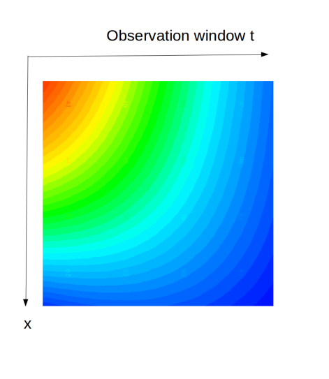
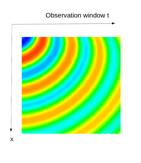
Figure 4. Plots of solutions. Left: Case (a). Right: Case (b).

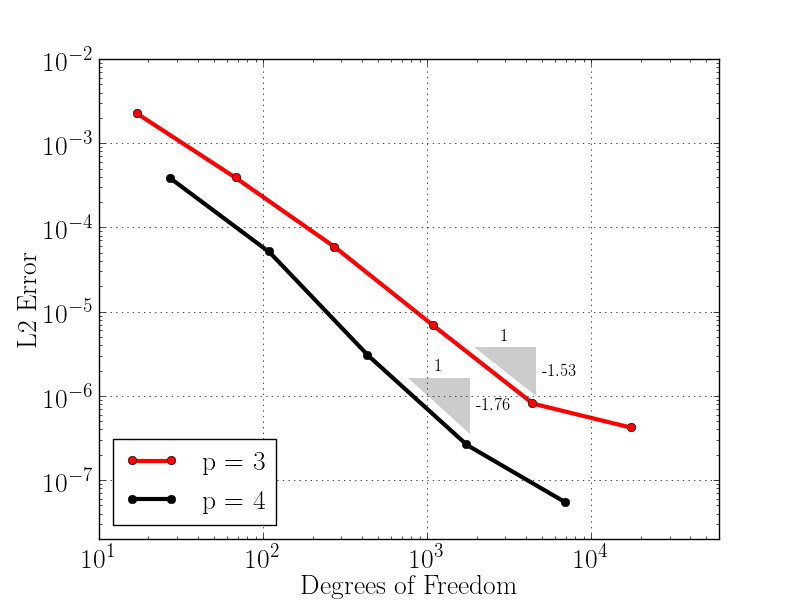
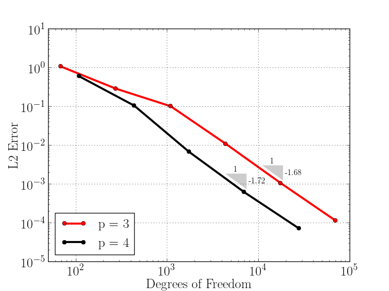
Figure 5. Rates of convergence. Left: Results from case (a) with the complex Gaussian solution. Right: Results from the case (b) with the wave packet of frequency $\omega=20$.

We report the observed rates of convergence for two problems: (a) The first case is when the exact solution is a complex Gaussian

$$u(x,t)=\frac{MT_{0}}{\sqrt{T_{0}^{2}-i\beta t}}e^{-\frac{x^{2}}{T_{0}^{2}-i\beta t}},$$ (5.1)

where $M,T_{0},$ and $\beta$ are fiber-dependent constants (see [26]). Our simulations used non-dimensionalized units of $M=T_{0}=1.5$ and $\beta=2.5$. (b) The second example uses an exact solution which is a wave packet traveling along the fiber whose in-packet oscillations are of moderately high wavenumber $\omega$, namely

$$u(x,t)=a_{0}e^{-\frac{x^{2}+t^{2}}{\omega^{2}}},$$ (5.2)

where the amplitude $a_{0}=(2/\omega^{2})^{1/4}$ and the wavenumber is $\omega=20$. Plots of solutions in either case are displayed in Figure 4.

The observed convergence rates are displayed in Figure 5 (the left plot shows results from case (a) and the right plot shows results from case (b). We experiment with $p=3$ and $p=4$ cases. For the ideal DPG method using the $U_{h}\times Q_{h}$ in (4.4), Theorem 4.3 implies that the convergence rate in terms of the number of degrees of freedom $n=O(h^{-2})$ is $O(n^{-s})$ where $s=(p-1)/2$. We observe from Figure 5 that in spite of reducing $Q_{h}$ to $\tilde{Q}_{h}$ and in spite of approximating $T$ by $T_{h}$, we continue to observe a rate higher than $s$. Namely, in the $p=3$ case, while we expected a rate of $s\leq 1$, the observed rate is $s\approx 1.5$. In the $p=4$ case, while the expected rate is $s\leq 1.5$, the observed rate is between $1.5$ and $2$. An improved error analysis explaining these observations is yet to be found.

Note the flattening out of the curves in left plot of Figure 5. This is due to conditioning issues. As with any method using second order derivatives, we should be wary of conditioning. Indeed, the DPG system with $p=3$ or $p=4$, after 4 or 5 uniform refinements, has a condition number in the vicinity of $O(10^{10})$. Therefore, the roundoff effect becomes apparent after we achieve an error threshold around $10^{-6}$ or $10^{-7}$. This is the cause of convergence curves flattening out in case (a). In case (b), due to $\omega=20$, we start with a higher error so the loss of digits due to conditioning issues is postponed.

Appendix A Abstract weak formulation

In this section, we consider a boundary value problem involving a general partial differential operator. We derive a mesh-dependent weak formulation of the boundary value problem and show that it is possible to identify sufficient conditions for its wellposedness. This section can be read independently of the remainder of the paper.

Let $\varOmega\subseteq\mathbb{R}^{d}$ be a bounded open set in $d\geq 1$ dimensions and let $k,l,m\geq 1$ be integers. Let $A$ be a differential operator such that $i$th component of $Au$ is

$$[Au]_{i}=\sum_{j=1}^{m}\sum_{|\alpha|\leq k}\partial^{\alpha}(a_{ij\alpha}u_{j}),$$ (A-a)

where $a_{ij\alpha}:\varOmega\to\mathbb{C}$ are functions for all $i=1,\ldots,l$, $j=1,\ldots,m,$ and all multi-indices $\alpha=(\alpha_{1},\ldots\alpha_{d})$ whose length is $|\alpha|=\alpha_{1}+\cdots+\alpha_{d}\leq k$. As usual, $\partial^{\alpha}=\partial_{1}^{\alpha_{1}}\cdots\partial_{d}^{\alpha_{d}}$. The formal adjoint of $A$ is given by

$$[A^{*}v]_{j}=\sum_{i=1}^{l}\sum_{|\alpha|\leq k}(-1)^{|\alpha|}\overline{a_{ji\alpha}}\,\partial^{\alpha}v_{j}.$$ (A.1)

We assume that the coefficients $a_{ij\alpha}$ are such that

$$A^{*}u\in\mathcal{D}^{\prime}(\varOmega)^{m}\quad\text{ for all }u\in L^{2}(\varOmega)^{l}.$$ (A-b)

For example, (A-b) is satisfied if $a_{ij\alpha}$ are smooth.

For any nonempty open subset $S\subseteq\varOmega,$ define the space

$$W(S)=\{u\in L^{2}(S)^{m}:Au\in L^{2}(S)^{l}\},$$ (A.2)

normed by $\|u\|_{W(S)}=\left(\|u\|_{S}^{2}+\|Au\|_{S}^{2}\right)^{1/2},$ and the space

$$W^{*}(S)=\{u\in L^{2}(S)^{l}:A^{*}u\in L^{2}(S)^{m}\},$$ (A.3)

normed by $\|u\|_{W^{*}(S)}=\left(\|u\|_{S}^{2}+\|A^{*}u\|_{S}^{2}\right)^{1/2}.$ Here and throughout, $(\cdot,\cdot)_{\varOmega}$ and $\|\cdot\|_{\varOmega}$ denote the inner product and the norm, respectively, in $L^{2}(\varOmega)$ or its Cartesian products. To simplify notation, we abbreviate $W=W(\varOmega)$, $W^{*}=W^{*}(\varOmega)$. Clearly these are inner product spaces.

Lemma A.1.

The spaces $W(S)$ and $W^{*}(S)$ are Hilbert spaces.

Proof.

Since the proofs for $W(S)$ and $W^{*}(S)$ are similar, we only show the first. Suppose $u_{n}$ is a Cauchy sequence in $W{{(S)}}$. Then $u_{n}$ is Cauchy in $L^{2}(S)^{m}$ and $Au_{n}$ is Cauchy in $L^{2}(S)^{l}$. Hence there is a $u\in L^{2}(S)^{m}$ and $f\in L^{2}(S)^{l}$ such that $\|u-u_{n}\|_{S}\to 0$ and $\|f-Au_{n}\|_{S}\to 0$. We will show that $u$ is in $W(S).$

Let $\phi\in\mathcal{D}(S)^{l}$. For each $w\in L^{2}(S)^{m}$, the distributional action of $Aw$ on $\bar{\phi}$, denoted by $\langle{Aw,\phi}\rangle_{\mathcal{D}(S)^{l}},$ equals $(w,A^{*}\phi)_{S}$. If $w$ is also in $W(S)$, then

$$(Aw,\phi)_{S}=\langle{Aw,\phi}\rangle_{\mathcal{D}(S)^{l}}=(w,A^{*}\phi)_{S}$$ (A.4)

for all $\phi$ in $\mathcal{D}(S)^{l}$. To complete the proof, we apply (A.4) with $w=u_{n}$ to get

$$\langle{Au,\phi}\rangle_{\mathcal{D}(S)^{l}} =(u,A^{*}\phi)_{S}=\lim_{n\to\infty}(u_{n},A^{*}\phi)_{S}=\lim_{n\to\infty}(Au_{n},\phi)_{S}=(f,\phi)_{S}$$

for all $\phi$ in $\mathcal{D}(S)^{l}$. Hence $Au=f$, and $u$ is in $W(S)$. ∎

Next, define bounded linear operators $D_{S}:W(S)\to W^{*}(S)^{\prime}$ and $D^{*}_{S}:W^{*}(S)\to W(S)^{\prime}$ by

$$\langle{D_{S}w,\tilde{w}}\rangle_{W^{*}(S)} =(Aw,\tilde{w})_{S}-(w,A^{*}\tilde{w})_{S},$$ (A.5)

$$\langle{D_{S}^{*}\tilde{w},w}\rangle_{W(S)} =(A^{*}\tilde{w},w)_{S}-(\tilde{w},Aw)_{S},$$ (A.6)

for all $w\in W(S)$ and $\tilde{w}\in W^{*}(S)$. When $S=\varOmega$, we abbreviate $D_{S}$ and $D^{*}_{S}$ to $D$ and $D^{*}$, respectively. Here, like in (A.4), and in the remainder, we use $\langle{\cdot,\cdot}\rangle_{X}$ to denote the action of a linear functional in $X^{\prime}$ on an element of $X$.

Next we will view $A:\mathop{\mathrm{dom}}(A)\subset L^{2}(\varOmega)^{m}\to L^{2}(\varOmega)^{l}$ as an unbounded linear operator, whose domain (denoted by $\mathop{\mathrm{dom}}(A)$) is chosen so that

$$\mathcal{D}(\varOmega)^{m}\subseteq\mathop{\mathrm{dom}}(A).$$ (A-c)

This implies that $A$ is a densely defined operator. Then, identifying the dual of (Cartesian products of) $L^{2}(\varOmega)$ with itself, recall that the adjoint $A^{*}:\mathop{\mathrm{dom}}(A^{*})\subset L^{2}(\varOmega)^{l}\to L^{2}(\varOmega)^{m}$ is a uniquely defined (unbounded) closed linear operator [3, 24] on $\mathop{\mathrm{dom}}(A^{*})=\{s\in L^{2}(\varOmega)^{l}:$ there is an $\ell\in L^{2}(\varOmega)^{m}$ such that $(Av,s)_{\varOmega}=(v,\ell)_{\varOmega}$ for all $v\in\mathop{\mathrm{dom}}(A)\},$ satisfying $(Av,\tilde{v})_{\varOmega}=(v,A^{*}\tilde{v})_{\varOmega}$ for all $v\in\mathop{\mathrm{dom}}(A)$ and $\;\tilde{v}\in\mathop{\mathrm{dom}}(A^{*}).$ Note that $\mathcal{D}(\varOmega)^{l}\subseteq\mathop{\mathrm{dom}}(A^{*})$. Note also that by an abuse of notation, we have used $A^{*}$ to denote both the differential operator in (A.1) and the adjoint operator of the unbounded $A$.

When $\mathop{\mathrm{dom}}(A)$ is endowed with the topology of $W(\varOmega)$, we call it $V$, i.e., although $V$ and $\mathop{\mathrm{dom}}(A)$ coincide as sets, $V$ has the topology of $W(\varOmega)$ and $\mathop{\mathrm{dom}}(A)$ has the topology of $L^{2}(\varOmega)^{m}$. Similarly, $\mathop{\mathrm{dom}}(A^{*})$ is called $V^{*}$ when it is endowed with the topology of $W^{*}(\varOmega)$. For the next result, recall that the left annihilator of any subspace $R$ of the dual space $X^{\prime}$ of any Banach space $X$ is defined by $\sideset{{}^{\perp}}{}{\mathop{R}}=\{w\in X:\langle{s^{\prime},w}\rangle_{X}=0\text{ for all }s^{\prime}\in R\}.$

Lemma A.2.

In the setting of (A-a), (A-b) and (A-c), we have $V^{*}=\sideset{{}^{\perp}}{}{\mathop{D(V)}}.$

Proof.

According to the (above-mentioned) definition of $\mathop{\mathrm{dom}}(A^{*})$, for any $\tilde{v}\in\mathop{\mathrm{dom}}(A^{*})=V^{*}$, there is an $\ell\in L^{2}(\varOmega)^{l}$ such that

$$(Av,\tilde{v})_{\varOmega}=(v,\ell)_{\varOmega},\qquad\forall v\in V.$$ (A.7)

Due to (A-c), we may choose $v$ in $\mathcal{D}(\varOmega)^{m}$. By (A-b), $A^{*}\tilde{v}$ is a distribution and by (A.7) this distribution is in $L^{2}(\varOmega)^{m}$ and equals $\ell.$ In particular, $\tilde{v}$ is in $W^{*}(\varOmega)$. Hence (A.5) is applicable, and in combination with (A.7) yields $\langle{Dv,\tilde{v}}\rangle_{W^{*}(\varOmega)}=(Av,\tilde{v})_{\varOmega}-(v,\ell)_{\varOmega}=0$ for all $v\in V$. Hence $\tilde{v}\in\sideset{{}^{\perp}}{}{\mathop{D(V)}}$ and we have proved that $V^{*}\subseteq\sideset{{}^{\perp}}{}{\mathop{D(V)}}$. The reverse containment is also easy to prove. ∎

We are interested in the boundary value problem of finding $u$ satisfying

$$Au=f,\qquad u\in\,V,$$ (A.8)

given $f\in L^{2}(\varOmega)^{l}$. Homogeneous boundary conditions are incorporated in $V.$ Consider the scenario where $\varOmega$ is partitioned into a mesh $\varOmega_{h}$ of finitely many open elements $K$ such that $\bar{\varOmega}=\cup_{K\in\varOmega_{h}}\bar{K}$. Here the index $h$ denotes $\max_{K\in\varOmega_{h}}\mathop{\mathrm{diam}}(K)$. Recall $D_{K}$ and $D_{K}^{*}$ by replacing $S$ by $K$ in (A.5) and (A.6). Additionally, set

$$W_{h} =\prod_{K\in\varOmega_{h}}W(K), (W_{h}^{*})^{\prime} =\prod_{K\in\varOmega_{h}}W^{*}(K)^{\prime}.$$ (A.9)

The spaces $W_{h}^{*}$ and $W_{h}^{\prime}$ are defined similarly. The component on an element $K$ of functions in such product spaces are indicated by placing $K$ as subscript, e.g., for any $w$ in $W_{h}$, the component of $w$ on element $K$ is denoted by $w_{K}$. Let $D_{h}:W_{h}\to(W_{h}^{*})^{\prime}$ be the continuous linear operator defined by

$$\langle{D_{h}w,v}\rangle_{W_{h}^{*}}=\sum_{K\in\varOmega_{h}}\langle{D_{K}w_{K},v_{K}}\rangle_{W^{*}(K)}$$

for all $w\in W_{h}$ and $v\in W_{h}^{*}$. To simplify notation, we abbreviate $\langle{D_{h}w,v}\rangle_{W_{h}^{*}}$ to $\langle{D_{h}w,v}\rangle_{h}$, i.e., duality pairing in $W_{h}^{*}$ is simply denoted by $\langle{\cdot,\cdot}\rangle_{h}$. For any $w\in W_{h}$, we denote by $A_{h}w$ the function obtained by applying $A$ to $w_{K}$, element by element, for all $K\in\varOmega_{h}$. The resulting function $A_{h}w$ is an element of $\Pi_{K\in\varOmega_{h}}L^{2}(K)^{l}$, which is identified to be the same as $L^{2}(\varOmega)^{l}$. The operator $A_{h}^{*}:W_{h}^{*}\to L^{2}(\varOmega)^{m}$ is defined similarly. Thus

$$\langle{D_{h}w,v}\rangle_{h}=(A_{h}w,v)_{\varOmega}-(w,A_{h}^{*}v)_{\varOmega}$$ (A.10)

for all $w\in W_{h}$ and $v\in W_{h}^{*}$.

Lemma A.3.

For all $w\in W$ and $v\in W^{*}$, we have $\langle{D_{h}w,v}\rangle_{h}=\langle{Dw,v}\rangle_{W}.$

Proof.

If $w\in W$ and ${{v}}\in W^{*}$, then $A_{h}w=Aw$ and $A_{h}^{*}{{v}}=A^{*}{{v}}$. Using this in (A.10), $\langle{D_{h}w,v}\rangle_{h}=(Aw,v)_{\varOmega}-(w,A^{*}v)_{\varOmega}=\langle{Dw,v}\rangle_{W^{*}}$ whenever $w$ is in $W$ and $v$ is in $W^{*}$. ∎

To derive the mesh-dependent weak formulation, multiply (A.8) by a test function $v\in W_{h}$ and apply the definition of $D_{K}$. Summing over all $K\in\varOmega_{h}$, we obtain $(u,A^{*}_{h}v)_{\varOmega}+\langle{D_{h}u,v}\rangle_{h}=(f,v)_{\varOmega}$ for all $v$ in $W_{h}^{*}$. Let

$$Q=\{r\in(W_{h}^{*})^{\prime}:\;\text{ there is a $v\in V$ such that }r=D_{h}v\}.$$ (A.11)

Setting $D_{h}u$ to be a new unknown $q$ in $Q$, we have thus derived the following weak formulation with $F(v)=(f,v)_{\varOmega}$.

Problem A.4.

Given any $F\in(W_{h}^{*})^{\prime},$  find $u\in L^{2}(\varOmega)^{m}$ and $q\in Q$ such that

$$(u,A_{h}^{*}v)_{\varOmega}+\langle{q,v}\rangle_{h}=F(v),\qquad\forall v\in W_{h}^{*}.$$

Theorem A.5.

In the setting of (A-a), (A-b) and (A-c), suppose

$$V=\sideset{{}^{\perp}}{}{\mathop{D^{*}(V^{*})}},\text{ and }$$ (A.12)

$$A:V\to L^{2}(\varOmega)^{l}\text{ is a bijection}.$$ (A.13)

Then, Problem A.4 is well posed. Moreover, if $F(v)=(f,v)_{\varOmega}$ for some $f\in L^{2}(\varOmega)^{l},$ then the unique solution $u$ of Problem A.4 is in $V,$ solves (A.8), and satisfies $q=D_{h}u$.

Before we prove this theorem, we must note how our assumptions allow a natural topology on $Q$. Specifically, (A.12) implies that $V$ is a closed subspace of $W$. It is also a closed subspace of $W_{h}$ since $W$ is continuously embedded in $W_{h}$. The same embedding also shows that the restriction of $D_{h}$ to $V$, denoted by $D_{h,V}:V\to(W_{h}^{*})^{\prime}$, is continuous. Note that $Q$ is the range of $D_{h,V}$. For any $r$ in $Q$, we use $D_{h,V}^{-1}(\{r\})$ to denote the pre-image of $r$, i.e., set of all $v\in V$ such that $r=D_{h}v.$ The continuity of $D_{h,V}$ implies that $D_{h,V}^{-1}(\{0\})$ is a closed subspace of $V$. Hence

$$\|q\|_{Q}=\inf_{v\in D_{h,V}^{-1}(\{q\})}\|v\|_{W}$$ (A.14)

is a norm on $Q$. This quotient norm makes $Q$ complete. The wellposedness result of Theorem A.5 is to be understood with $Q$ endowed with this norm.

A.1. A proof of wellposedness

We now give a proof of Theorem A.5. Recall that the right annihilator of any subspace $S\subseteq X$ is defined by ${S}^{\perp}=\{w^{\prime}\in W^{\prime}:\langle{w^{\prime},s}\rangle_{W}=0\text{ for all }s\in S\}.$ The next lemma is used below to prove uniqueness.

Lemma A.6.

If (A.12) holds, then $D_{h}V\subseteq{(V^{*})}^{\perp}.$

Proof.

Let $w\in V\subseteq W_{h}$. Then for any $\tilde{v}\in V^{*}$, the functional $D_{h}w\in(W_{h}^{*})^{\prime}$ satisfies $\langle{D_{h}w,\tilde{v}}\rangle_{h}=\langle{Dw,\tilde{v}}\rangle_{W^{*}}$ by Lemma A.3. But $\langle{Dw,\tilde{v}}\rangle_{W^{*}}=-\overline{\langle{D^{*}\tilde{v},w}\rangle}_{W}=0$ since (A.12) shows that $w\in\sideset{{}^{\perp}}{}{\mathop{D^{*}(V^{*})}}$. Hence $D_{h}w\in{(V^{*})}^{\perp}$. ∎

Proof of Theorem A.5.

We verify the uniqueness and inf-sup conditions of the Babuška theory to obtain wellposedness. To verify the uniqueness condition, we must prove that if

$$(u,A_{h}^{*}v)_{\varOmega}+\langle{q,v}\rangle_{h}=0,\qquad\forall v\in W_{h}^{*},$$ (A.15)

then $u$ and $q$ vanishes. Since $q=D_{h}z$ for some $z\in V$, by virtue of Lemma A.6, $\langle{q,v}\rangle_{h}=0$ for any $v$ in $V^{*}$. Hence (A.15) implies

$$(u,A_{h}^{*}v)_{\varOmega}=0,\qquad\forall v\in V^{*}.$$ (A.16)

In particular, since $\mathcal{D}(\varOmega)^{l}\subseteq V^{*}$, this implies that $Au=0$ and therefore $u\in W$. Hence (A.5) and (A.16) imply $\langle{Du,v}\rangle_{W^{*}}=0$, or equivalently $\langle{D^{*}v,u}\rangle_{W}=0$ for all $v\in V^{*}$. Thus $u\in\sideset{{}^{\perp}}{}{\mathop{D^{*}(V^{*})}}=V$. The bijectivity of $A:V\to L^{2}(\varOmega)^{l}$ then implies that $u=0$. Returning to (A.15) and setting $u=0$, we see that $\langle{q,v}\rangle_{h}=0$ for all $v\in W_{h}^{*}$, so $q=0$ as well.

It only remains to prove the inf-sup condition

$$\|w\|_{W_{h}^{*}}\leq C_{1}\sup_{0\neq x\in X}\frac{|b(x,w)|}{\;\|x\|_{X}},$$ (A.17)

where $X=L^{2}(\varOmega)^{m}\times Q$ and $b((u,q),w)=(u,A_{h}^{*}w)_{\varOmega}+\langle{q,w}\rangle_{h}$. Given any $w\in W_{h}^{*}\subseteq L^{2}(\varOmega)^{l}$, we use the bijectivity of $A:V\to L^{2}(\varOmega)^{l}$ and the Banach Open Mapping theorem to obtain a $v$ in $V$ satisfying $Av=w,$ and $\|v\|_{W}\leq C\|w\|_{W_{h}^{*}}.$ Then, setting $z=v+A_{h}^{*}w$ and $r=D_{h}v,$ we have $\|r\|_{Q}\leq\|v\|_{W}\leq C\|w\|_{W_{h}^{*}}$ and $\|z\|_{\varOmega}\leq(C+1)\|w\|_{W_{h}^{*}}$. Hence

$$\|w\|_{W_{h}^{*}}^{2} =(A_{h}v,w)_{\varOmega}+(A^{*}_{h}w,A^{*}_{h}w)_{\varOmega}=(v+A^{*}_{h}w,A^{*}_{h}w)_{\varOmega}+\langle{D_{h}v,w}\rangle_{h}$$

$$=\|(z,r)\|_{X}\;\frac{b((z,r),\,w)}{\|(z,r)\|_{X}}\;\leq\;C_{1}\|w\|_{W_{h}^{*}}\;\sup_{0\neq x\in X}\frac{|b(x,w)|}{\;\|x\|_{X}},$$

where $C_{1}$ depends only on $C$. Hence (A.17) follows. ∎

Remark A.7.

Various elements of the arguments used in this proof are well-known in the DPG literature – see e.g., [12, § 6.2]. A generalization of these ideas to make a unified theory for DPG approximations of all Friedrichs systems was attempted in [4]. However, [4, equation (2.17)] is not correct (a counterexample is easily furnished by the Laplace example) and unfortunately that equation is used in [4, Lemma 2.4 and Corollary 2.5] to prove the existence of a solution for Problem A.4. The above proof provides a corrigendum to [4] and shows that the results claimed there for symmetric Friedrichs systems are indeed correct for operators of the form (A-a) with $k=1$ and with $V$ and $V^{*}$ set respectively to the null spaces of the operators $B-M$ and $B+M^{*}$ defined there.

Remark A.8.

The above analysis is applicable beyond Friedrichs systems as the example of Schrödinger equation shows. “Instead of working with one equation of higher than first order,” writes Friedrichs in his early work [19], “we prefer to work with a system of equations of first order.” We have already noted the difficulties in reformulating the Schrödinger equation as a first order system. The modern theory of Friedrichs systems (for operators of the form (A-a) with $l=m$) starts with the assumption that $\|(A+A^{*})\phi\|_{\varOmega}\leq C\|\phi\|_{\varOmega}$ for all $\phi\in\mathcal{D}(\varOmega)^{l}$ – see [17, equation (T2)]. This assumption does not hold for the Schrödinger operator.

A.2. An alternate proof of wellposedness

Another proof of Theorem A.5 can be given using the following two lemmas.

Lemma A.9.

$V^{*}=\{y\in W_{h}^{*}:\;\langle{q,y}\rangle_{h}=0\text{ for all }q\in Q\}.$

Proof.

If $y\in V^{*},$ then for any $z\in V,$ using Lemmas A.3 and A.2, we have $\langle{D_{h}z,y}\rangle_{h}=\langle{Dz,y}\rangle_{W^{*}}=0,$ i.e., $\langle{q,y}\rangle_{h}=0$ for all $q\in Q.$

To prove the reverse containment, let $y\in W_{h}^{*}$ satisfy $\langle{D_{h}z,y}\rangle_{h}=0$ for all $z\in V.$ For any $\phi\in\mathcal{D}(\varOmega)^{m}$, the distribution $A^{*}y$ satisfies $\langle{A^{*}y,\phi}\rangle_{\mathcal{D}(\varOmega)^{m}}=(y,A\phi)_{\varOmega}=(A_{h}^{*}y,\phi)_{\varOmega}+\overline{\langle{D_{h}\phi,y}\rangle}_{h}$. The last term is zero, because by (A-c), $\mathcal{D}(\varOmega)^{m}\subseteq\mathop{\mathrm{dom}}(A)=V$. Hence $A^{*}y=A_{h}^{*}y$ and $y$ is in $W^{*}$. Thus by Lemma A.3, $\langle{D_{h}z,y}\rangle_{h}=\langle{Dz,y}\rangle_{W}=0$, so $y\in\sideset{{}^{\perp}}{}{\mathop{D(V)}}$. Hence $y$ is in $V^{*}$ by Lemma A.2. ∎

Lemma A.10.

Suppose (A.12) holds. Then, for all $q\in Q$,

$$\inf_{v\in D_{h,V}^{-1}(\{q\})}\|v\|_{W}\;=\sup_{0\neq y\in W_{h}^{*}}\frac{|\langle{q,y}\rangle_{h}|}{\quad\|y\|_{W_{h}^{*}}}.$$

Proof.

The supremum, denoted by $s$, is attained by the function $\tilde{u}_{q}$ in $W_{h}^{*}$ satisfying

$$(A_{h}^{*}\tilde{u}_{q},A_{h}^{*}y)_{\varOmega}+(\tilde{u}_{q},y)_{\varOmega}=-\langle{q,y}\rangle_{h},\qquad\forall y\in W_{h}^{*},\text{ and }$$ (A.18)

$$s=\|\tilde{u}_{q}\|_{W_{h}^{*}}.$$ (A.19)

Choosing $y\in\mathcal{D}(\varOmega)^{l}$ in (A.18), we conclude that the distribution $A(A_{h}^{*}\tilde{u}_{q})$ is in $L^{2}(\varOmega)^{l}$. Hence (A.10) is applicable with $w=A_{h}^{*}\tilde{u}_{q}$ and we obtain

$$A_{h}A_{h}^{*}\tilde{u}_{q}+\tilde{u}_{q} =0$$ (A.20a)

$$D_{h}A_{h}^{*}\tilde{u}_{q} =q.$$ (A.20b)

Now let $u_{q}=A_{h}^{*}\tilde{u}_{q}$. Then (A.20a) implies $A_{h}u_{q}=-\tilde{u}_{q}$, which implies $A_{h}^{*}A_{h}u_{q}=-A_{h}^{*}\tilde{u}_{q}=-u_{q}$. Combining with (A.20b), we have

$$A_{h}^{*}A_{h}u_{q}+u_{q} =0$$ (A.21a)

$$D_{h}u_{q} =q.$$ (A.21b)

Next, we show that $u_{q}$ is in $V$. By (A.12), it suffices to prove that $u_{q}\in\sideset{{}^{\perp}}{}{\mathop{D^{*}(V^{*})}}$. For any $\tilde{v}$ in $V^{*},$ we have, using Lemma A.3, $\langle{D^{*}\tilde{v},u_{q}}\rangle_{W}=-\overline{\langle{Du_{q},\tilde{v}}\rangle}_{W^{*}}=-\overline{\langle{D_{h}u_{q},\tilde{v}}\rangle}_{h}=-\overline{\langle{q,\tilde{v}}\rangle}_{h}$. The last term is zero because $q=D_{h}z$ for some $z\in V$ and $\langle{q,\tilde{v}}\rangle=\langle{Dz,\tilde{v}}\rangle_{W^{*}}=0$ by Lemma A.2. Hence $u_{q}\in\sideset{{}^{\perp}}{}{\mathop{D^{*}(V^{*})}}=V.$

The infimum of the lemma is $\|q\|_{Q}.$ By virtue of (A.19), to complete the proof, it suffices to show that $\|q\|_{Q}=\|u_{q}\|_{W}=\|\tilde{u}_{q}\|_{W_{h}^{*}}.$ The last equality is obvious from $u_{q}=A_{h}^{*}\tilde{u}_{q}$ and $A_{h}u_{q}=-\tilde{u}_{q}$, hence we need only show that $\|q\|_{Q}=\|u_{q}\|_{W}$. Standard variational arguments show that the infimum defining $\|q\|_{Q}$ is attained by a unique minimizer $v_{q}\in V$ satisfying $\|q\|_{Q}=\|v_{q}\|_{W}$, $D_{h}v_{q}=q$ and $(A_{h}v_{q},A_{h}v)_{\varOmega}+(v_{q},v)_{\varOmega}=0$ for all $v\in D_{h,V}^{-1}(\{0\}).$ Choosing a $v$ in $\mathcal{D}(K)$ (whose extension by zero is in $D_{h,V}^{-1}(\{0\})$), we conclude that distribution $A^{*}(A_{h}v_{q})|_{K}$ is in $L^{2}(K)^{m}$ for any $K\in\varOmega_{h}$. Therefore $A_{h}^{*}A_{h}v_{q}$ is in $L^{2}(\varOmega)^{m}$. In view of (A.21), this means that $v_{q}=u_{q}$. ∎

Second proof of Theorem A.5.

According to [5, Theorem 3.3], it suffices to prove that there are positive constants $c_{0},\hat{c}$ such that

$$c_{0}\|u\|_{\varOmega}\leq\sup_{0\neq y\in Y_{0}}\frac{|(u,A_{h}^{*}y)_{\varOmega}|}{\|y\|_{W_{h}^{*}}} \forall\; u\in L^{2}(\varOmega)^{m},$$ (A.22)

$$\hat{c}\,\|q\|_{Q}\leq\sup_{0\neq y\in W_{h}^{*}}\frac{|\langle{q,y}\rangle_{h}|}{\quad\|y\|_{W_{h}^{*}}} \forall\; q\in Q,$$ (A.23)

where $Y_{0}=\{y\in W_{h}^{*}:\;\langle{q,y}\rangle_{h}=0\text{ for all }q\in Q\}.$

Since (A.23) follows with $\hat{c}=1$ from Lemma A.10, we only need to prove (A.22). First note that since $V$ is closed (by (A.12)), $A$ is a closed operator. By (A.13), the range of $A$ is closed. By the Closed Range Theorem for closed operators, range of $A^{*}$ is closed. Also, the well-known identity $\ker(A^{*})={\mathop{\mathrm{ran}}(A)}^{\perp}$, in combination with (A.13), implies that $A^{*}$ is injective. Hence there exists a $C>0$ such that

$$C\|y\|_{\varOmega}\leq\|A^{*}y\|_{\varOmega}\qquad\forall y\in\mathop{\mathrm{dom}}(A^{*})=V^{*}.$$ (A.24)

This implies the following inf-sup condition:

$$C\|y\|_{W^{*}}\leq\sup_{u\in L^{2}(\varOmega)^{m}}\frac{|(u,A^{*}y)_{\varOmega}|}{\|u\|_{\varOmega}}\qquad\forall y\in V^{*}.$$

To complete the proof, we note that by standard arguments the order of arguments in the inf and sup may be reversed to get

$$\inf_{u\in L^{2}(\varOmega)^{m}}\sup_{y\in V^{*}}\frac{|(u,A^{*}y)_{\varOmega}|}{\;\;\|u\|_{\varOmega}\;\|y\|_{W^{*}}}\;=\;\inf_{y\in V^{*}}\sup_{u\in L^{2}(\varOmega)^{m}}\frac{|(u,A^{*}y)_{\varOmega}|}{\;\;\|u\|_{\varOmega}\;\|y\|_{W^{*}}}\geq C.$$

By Lemma A.9, $Y_{0}=V^{*}$, thus completing the proof of (A.22). ∎

Remark A.11.

The idea behind Lemma A.10 (to consider the two related problems (A.20) and (A.21), one with essential boundary conditions and the other with natural boundary conditions) was first presented in [5, 6], tailored to the specific needs of a Maxwell problem. A generalization for first order operators was presented later in [28]. The argument to prove (A.22) using the Closed Range Theorem, was first presented for the case of first order Sobolev spaces in [5, Theorem 6.6].

References

• [1] G. P. Agrawal, Nonlinear Fiber Optics, Fifth Edition, Academic Press, Waltham, Massachusetts, USA, 2012.
• [2] J. Bramwell, L. Demkowicz, J. Gopalakrishnan, and W. Qiu, A locking-free $hp$ DPG method for linear elasticity with symmetric stresses, Numer. Math., 122 (2012), pp. 671–707.
• [3] H. Brezis, Functional analysis, Sobolev spaces and Partial Differential Equations, Universitext, Springer, 2011.
• [4] T. Bui-Thanh, L. F. Demkowicz, and O. Ghattas, A unified discontinuous Petrov-Galerkin method and its analysis for Friedrichs’ systems, SIAM Journal on Numerical Analysis, 51 (2013), pp. 1933–1958.
• [5] C. Carstensen and L. F. Demkowicz and J. Gopalakrishnan, Breaking Spaces and Forms for the DPG Method and Applications Including Maxwell Equations, Computers and Mathematics with Applications, 72 (2016), p. 494–522.
• [6] C. Carstensen, L. Demkowicz, and J. Gopalakrishnan, DPG methods for Maxwell equations, in Oberwolfach Reports: Computational Engineering, S. C. Brenner, C. Carstensen, L. Demkowicz, and P. Wriggers, eds., vol. 43/2015, September 2015.
• [7] C. Carstensen, L. F. Demkowicz, and J. Gopalakrishnan, A posteriori error control for DPG methods, SIAM J. Numer. Anal., 52 (2014), pp. 1335–1353.
• [8] P. G. Ciarlet, The Finite Element Method for Elliptic Problems, Society for Industrial and Applied Mathematics (SIAM), 2 ed., 2002.
• [9] W. Dahmen, C. Huang, C. Schwab, and G. Welper, Adaptive Petrov-Galerkin methods for 1st order transport equations, SIAM J. Numer. Anal., 50 (2012), pp. 2420–2445.
• [10] L. Demkowicz and J. Gopalakrishnan, A class of discontinuous Petrov-Galerkin methods. Part I: The transport equation, Computer Methods in Applied Mechanics and Engineering, 199 (2010), pp. 1558–1572.
• [11] L. Demkowicz and J. Gopalakrishnan, Analysis of the DPG method for the Poisson equation, SIAM J. Numer. Anal., 49 (2011), pp. 1788–1809.
• [12] L. Demkowicz, J. Gopalakrishnan, I. Muga, and J. Zitelli, Wavenumber explicit analysis for a DPG method for the multidimensional Helmholtz equation, Computer Methods in Applied Mechanics and Engineering, 213/216 (2012), pp. 126–138.
• [13] L. Demkowicz and N. Heuer, Robust DPG method for convection-dominated diffusion problems, SIAM J. Numer. Anal., 51 (2013), pp. 2514–2537.
• [14] L. F. Demkowicz and J. Gopalakrishnan, A class of discontinuous petrov-galerkin methods. part ii: Optimal test functions, Numerical Methods for Partial Differential Equations, 27 (2011), pp. 70–105.
• [15] T. E. Ellis, J. Chan, and L. F. Demkowicz, Robust DPG methods for transient convection-diffusion, ICES Report, The Institute for Computational Engineering and Sciences, The University of Texas at Austin, 15-21 (2015).
• [16] T. E. Ellis, L. F. Demkowicz, J. L. Chan, and R. D. Moser, Space-time DPG: Designing a method for massively parallel CFD, ICES Report, The Institute for Computational Engineering and Sciences, The University of Texas at Austin, 14-32 (2014).
• [17] A. Ern, J.-L. Guermond, and G. Caplain, An intrinsic criterion for the bijectivity of Hilbert operators related to Friedrichs’ systems, Communications in Partial Differential Equations, 32 (2007), pp. 317–341.
• [18] L. C. Evans, Partial Differential Equations, Graduate Studies in Mathematics vol. 19, American Mathematical Society, Providence, Rhode Island, USA, 1998.
• [19] K. Friedrichs, Symmetric positive linear differential equations, Comm. Pure Appl. Math., 11 (1958), pp. 333–418.
• [20] F. Fuentes, B. Keith, L. F. Demkowicz, and S. Nagaraj, Orientation embedded high order shape functions for the exact sequence elements of all shapes, Computers and Mathematics with Applications, 70 (2015), pp. 353–458.
• [21] J. Gopalakrishnan and W. Qiu, An analysis of the practical DPG method, Math. Comp., 83 (2014), pp. 537–552.
• [22] B. Keith, F. Fuentes, and L. F. Demkowicz, The DPG methodology applied to different variational formulations of linear elasticity, Computer Methods in Applied Mechanics and Engineering, 309 (2016), pp. 579–609.
• [23] S. Kesavan, Topics in Functional Analysis and Applications, Wiley Eastern Limited, Bombay, 1989.
• [24] J. T. Oden and L. F. Demkowicz, Applied Functional Analysis, CRC Press, Boca Raton, FL, USA, 2010.
• [25] N. V. Roberts, T. Bui-Thanh, and L. F. Demkowicz, The DPG Method for the Stokes Problem, Computers and Mathematics with Applications, 67 (2014), pp. 966–995.
• [26] J. K. Shaw, Mathematical Principles of Optical Fiber Communication, CBMS-NSF Regional Conference Series in Applied Mathematics (76), SIAM: Society for Industrial and Applied Mathematics, 2004.
• [27] T. Tao, Nonlinear Dispersive Equations, CBMS Regional Conference Series in Mathematics vol. 106, Published for the Conference Board of the Mathematical Sciences, Washington, DC by the American Mathematical Society, 2006.
• [28] C. Wieners, The skeleton reduction for finite element substructuring methods, ENUMATH 2015 Proceedings, ((to appear) 2016).