A model with Darwinian dynamics on a rugged landscape

Abstract

We discuss the population dynamics with selection and random diffusion, keeping the total population constant, in a fitness landscape associated with Constraint Satisfaction, a paradigm for difficult optimization problems. We obtain a phase diagram in terms of the size of the population and the diffusion rate, with a glass phase inside which the dynamics keeps searching for better configurations, and outside which deleterious ‘mutations’ spoil the performance. The phase diagram is analogous to that of dense active matter in terms of temperature and drive.

I Introduction

Optimization problems – finding the minima of complicated functions – are ubiquitous in science. Statistical Mechanics has proved to be an extremely powerful tool to analyze such problems and the associated algorithms. This is based on the recognition that the energy function of glassy systems are archetypical rugged landscapes, and that the annealing and aging of real glasses are nature’s way to minimize the energy. Simulating the annealing procedure for artificial optimization problems is a robust and quite effective method Kirkpatrick .

Darwinian dynamics may be viewed as an alternative method to optimize a function – in this case maximizing the ‘fitness’ – clearly also widespread in nature. This has been long recognized, and the literature on artificial ‘Genetic Algorithms’ is vast genetic . The principle is rather different from that of annealing: instead of the algorithm searching actively for a better situation (a ‘Lamarckian’ strategy), it just produces ‘clones’ that mutate randomly and are later selected according to their fitness. Because the connection between Darwinian dynamics and physical evolution is less obvious than in the case of annealing, the implications of physics to such problems has been much less studied. Although there have been statistical mechanical models of evolution (see, for example pedersen_long_1981 ; sibani_evolution_1999 ; seetharaman_evolutionary_2010 ; saakian_eigen_2004 ; saakian_evolutionary_2009 ; saakian_solvable_2004 ) using the knowledge of universal glassy features has been much less exploited franz_evolutionary_1993 .

Evolutionary programs appear naturally in physics when one models the (imaginary-time) Schroedinger Equation, a technique known as ‘Diffusion Monte Carlo’ anderson , and also in the efficient calculation of large deviations giardina , but they may of course also be used as an alternative to Simulated Annealing for the minimization of any cost function. Evolutionary dynamics has also been studied per se: the Quasispecies Model eigen being perhaps the best-known example. In these three cases, the better understood situation is the limit of large number of individuals. However, as we shall argue below, when the dynamics takes place in a rugged landscape, the consequences of the finite size of the population become important after a short (logarithmic in the size) time-scale. This leads us to studying a dynamics in which the number of individuals $N$ is finite, and for simplicity is kept fixed by randomly decimating the population: a Moran process.

The dynamics of a population of $N$ individuals reproducing and undergoing random mutations and selection has long been recognized to bear a resemblance with a system driven by a ‘fitness potential’, with an element of ‘noise’ given by random fluctuations that are larger, the smaller the total population (see, e.g. crow_introduction_1970 ; peliti_introduction_1997 ). However, the stochastic dynamics of a system in contact with a thermal bath satisfy the relation of ‘detailed-balance’ – the condition that the bath is itself in thermal equilibrium – obviously not applicable in general to an evolutionary dynamics with mutation and selection. A known exception happens when the population is dominated by a single mutant at any time, whose identity changes in rare and rapid ‘sweeps’ in which a new mutant fixes sella_application_2005 ; mustonen_fitness_2010 , see Fig. 4c. It turns out that in that special case berg_stochastic_2003 ; berg_adaptive_2004 ; sella_application_2005 ; barton_application_2009 , there is a correspondence that we shall exploit to understand some features of the phase diagram.

In this paper we shall study the Darwinian dynamics in an archetypical constraint optimization problem (Satisfiability: KSAT and XORSAT). Our purpose is not to propose this model as a relevant metaphor for biology (there are many references on this, see for example pedersen_long_1981 ; sibani_evolution_1999 ; seetharaman_evolutionary_2010 ; saakian_eigen_2004 ; saakian_evolutionary_2009 ; saakian_solvable_2004 ), but rather to work out the details in a nontrivial case. A complete analytic solution for the population dynamics in these models is perhaps possible, but seems like a daunting task.

II The Model

We shall consider a population of individuals assumed to be independent, their internal states being denoted $a=1,...,2^{L}$’. Each has on average $\lambda_{a}$ offspring per unit time. The total number $N$ is kept constant – or in some cases slowly varying – by decimating or ‘cloning’ randomly chosen individuals at the necessary rate, a Moran process moran_statistical_1962 . The probability of mutation per generation a state $a$ to a state $b$ is $\mu_{ab}$, so that mutation times are random with average $\tau_{ab}=1/\left(\lambda_{a}\mu_{ab}\right)$. In the literature, either the probabilities $\mu_{ab}$ or the times $\tau_{ab}$ are often taken identical for all allowed mutations. We shall adopt here $\tau_{ab}=\tau_{0}\;\forall{ab}$

The evolution is described by a time-dependent distribution of types $\{n_{1},...n_{2^{L}}\}(t)$, with $\sum_{i}n_{a}(t)=N$. Initial conditions need to be specified, such as a population containing a single type, or a random selection of states for the $N$ individuals. We represent the internal state of an individual using Boolean variables: ${\bf s}^{a}=\{s_{1}^{a},...,s_{L}^{a}\}$ taking values $s_{i}^{a}=0,1$. The fitness functions we use are standard spin-glass benchmarks, whose landscape properties have been extensively studied kauffman_metabolic_1969 . It is constructed as follows: there are $\alpha L$ clauses $\nu$ with $K=3$ variables, of the form $(s_{i_{1}^{\nu}}\vee\overline{s_{i_{2}^{\nu}}}\vee s_{i_{3}^{\nu}})$ where both the $(i_{1}^{\nu},i_{2}^{\nu},i_{3}^{\nu})$ chosen for each clause – and the fact that the variable is negated or not – are decided at random once and for all. The Random K-SAT and Random Xor-SAT take the form, for example:

OUTPUT = $(s_{18}\vee\overline{s_{3}}\vee s_{43})\wedge(s_{1}\vee s_{45}\vee\overline{s_{31}})...\wedge(\overline{s_{51}}\vee s_{7}\vee\overline{s_{8}})$   (SAT)

OUTPUT = $(s_{18}\veebar\overline{s_{3}}\veebar s_{43})\wedge(s_{1}\veebar s_{45}\veebar\overline{s_{31}})...\wedge(\overline{s_{51}}\veebar s_{7}\veebar\overline{s_{8}})$    (XorSAT)

If we assume that each clause has a multiplicative effect on the reproduction rate $\lambda$, this suggests we use an additive form for $E$

$$-\ln\lambda=\frac{1}{L}\sum_{a=1}^{\alpha L}[\mbox{error in clause }\nu]\equiv\frac{1}{L}E$$ (1)

The factor $\frac{1}{L}$ sets the scale. We work in a regime with $\alpha=6$: for such a number of clauses the system virtually never has a solution where all clauses are satisfied, i.e. $E>0$. The landscape is rugged and the minima are separated and extremely hard to find.

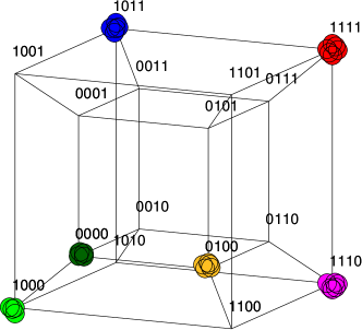
Figure 3: Genetic algorithm for SAT or XORSAT on the 4-dimensional hypercube. Each vertex has a given fitness value. Individuals reproduce with the rate determined by the vertex they are in, and mutate by diffusing to connected vertices.

The dynamics of the $N$ individuals, each identified by a vector ${\bf s}^{individual}$ is obtained by flipping randomly one of their components, in other words it is a diffusion on $L$ dimensional hypercube (Fig 3), where they reproduce or die according to the SAT or XORSAT fitness rule.

III A brief digression: the House of Cards Model

In order to see which are the good state parameters, and also to make this discussion less abstract, we shall first briefly review a concrete example about which much is known: the ‘House of Cards’ model kingman . We consider again states $a=1,...,2^{L}$ with log-fitnesses $\ln\lambda=-E/L$ distributed according to a Gaussian distribution (a choice inspired by the Random Energy Model derrida_random-energy_1980 ; neher_emergence_2013 , see below).

$$p(E) = {\cal L}e^{-E^{2}/2L}\hskip 28.45274pt\bar{p}(\lambda)=\frac{dE}{d\lambda}\;p(E)$$ (2)

The mutation rates $\mu_{ab}$ are identical for all pairs $ab$ with $\mu=\sum_{b}\mu_{ab}$, so an individual may jump between any two states.

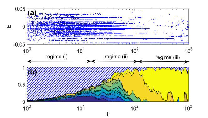
Figure 1: Evolution in the REM House-of-Cards model. (a) The energy of individuals. For clarity only 1 in 20 individuals is shown. (b) Evolution of the largest sub-populations, as in Fig. 4. Model parameters $N=500,\,L=2500,\,\mu=1/50$.

The evolution of this system is depicted in Fig 1, where initially each individual is chosen randomly. The system traverses through several regimes:

i) Continuous population: essentially all the population is in states $a$ such that $1\ll n_{a}\ll N$, for all other states $n_{a}=0$. One may treat the problem in terms of a continuous approximation $\rho(\lambda)$ corresponding to the fraction of individuals having $\lambda_{a}$ between contained between $\lambda$ and $\lambda+d\lambda$, using the Replicator Equation sigmund . We have:

$$\dot{\rho}(\lambda)=[\lambda\left(1-\mu\right)-\langle\lambda\rangle]\rho(\lambda)+\mu\lambda\bar{p}(\lambda)\hskip 42.67912ptwith\hskip 42.67912pt\langle\lambda\rangle=\int d\lambda\,\rho(\lambda)\,\lambda$$ (3)

where $\mu$ is the total probablity of mutating out of the interval $[\lambda,\lambda+d\lambda]$, and $\bar{p}(\lambda)$ is the density of states.

ii) Concurrent mutations regime desai_beneficial_2007 : Finite population size effects cannot be neglected even if the population starts at regime (i), because they begin to show up at times of order $\ln N$. Here a finite fraction of all individuals are concentrated in a finite number of types (Fig. 1) competing for domination (strong clonal interference). (See desai_beneficial_2007 ; rouzine_solitary_2003 ; rouzine_traveling-wave_2008 and good_distribution_2012 , especially Refs. [23-29] therein).

iii) Successional Mutation Regime: The system settles into a regime in which the majority of individuals belong to a single type. Some of these individuals mutate, most often deleteriously, and die, accounting for a constantly renewed population ‘cloud’ of order $\mu N$ outside the dominant sub-population. Every now and then, an individual mutates to a state that is more fit, in which case it may spread in the population until completely taking over (fixation). There are, in addition, events in which the entire population may get fixated to a mutation that is (slightly) less fit: these extinction events are exponentially rare in $N$. In this regime, it is easy to compute the probability for a new mutation to appear and fix in an interval of time $\delta t$, large with respect to the fixation time, small compared to the time between successive fixations crow_introduction_1970 :

$$P({\mbox{fixed in }}a\to{\mbox{fixed in }}b)\equiv P(a\rightarrow b)=N\lambda_{a}\mu_{ab}\delta t\;\frac{\frac{\lambda_{a}}{\lambda_{b}}-1}{(\frac{\lambda_{a}}{\lambda_{b}})^{N}-1}=N\lambda_{a}\mu_{ab}\delta t\;\frac{e^{\left(E_{b}-E_{i}\right)/L}-1}{e^{\left(E_{b}-E_{a}\right)N/L}-1}.$$ (4)

where

$$E_{a}\equiv-L\ln\lambda_{a}\>,$$ (5)

will turn out to play a role analogous to that of an energy. The normalization is chosen to make quantities of interest, such are changes in fitness, of order one. (Here we have assumed that $\mu L$ is small, so we have neglected the ‘cloud’ of deleterious mutations.) A population will evolve in this regime whenever mutations are rare mustonen_fitness_2010 ; mustonen_molecular_2008 because few useful mutations are offered in any generation .

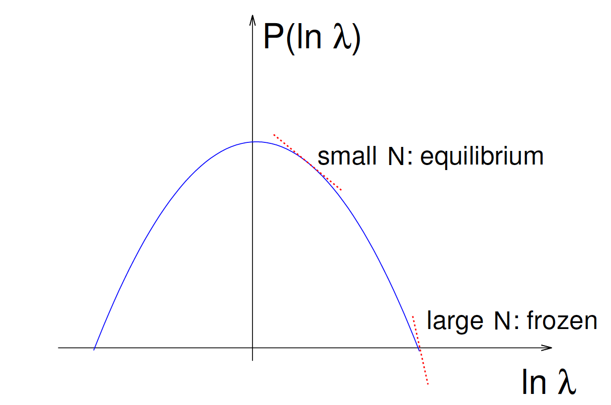
Figure 2: Equilibrium for the REM/House of Cards model.

Emergence of Detailed Balance in the successional regime

In the context of the House-of-Cards model, consider now for the successional mutation regime the ‘meta-dynamics’ of the dominant sub-population, considered as a single entity, neglecting the relatively short times in which the system is not concentrated into a single type (the fixation processess). Since in this example $\mu_{ab}=\mu_{ba}$:

$$\frac{P(a\to b)}{P(b\to a)}=\left(\frac{\lambda_{b}}{\lambda_{a}}\right)^{N-2}=e^{-(N-2)[\ln\lambda_{a}-\ln\lambda_{b}]}=e^{-\frac{N-2}{L}[E_{b}-E_{a}]}$$ (6)

This corresponds to a process with detailed balance and temperature $T=\frac{L}{N-2}$ and energies $E_{a}$ berg_adaptive_2004 ; berg_stochastic_2003 ; sella_application_2005 . In what follows we focus on large $N$, and dropping $O\left(1/N\right)$ corrections we write $T=\frac{L}{N}$. At very long times, the system will reach a distribution

$$P({\mbox{dominant type at }}a)=\frac{e^{-E_{a}/T}}{\sum_{b}e^{-E_{b}/T}}$$ (7)

Finding the stationary distribution has been reduced to the solution of the equilibrium Random Energy Model derrida_random-energy_1980 , (see neher_emergence_2013 and cammarota_spontaneous_2014 ). In particular, we conclude that, depending on the value of $N$, at very long times the system will equilibrate to either a ‘liquid’ phase (for $N/L<\ln 2$) or a ‘frozen’ phase (for $N/L>\ln 2$), see Fig. 2: in the former random extinction events stop the system from converging to the optimum level of fitness, while in the latter this level is at long times reached. A feature we find here, and is a general fact, is that even if the dynamics satisfy detailed balance, and are hence able in principle to equilibrate, this takes place at unrealistically long times.

The qualitative features of the population at different times has long been known, the similarity of the role played by fluctuations due to finite population size with thermal fluctuations has also been noted long ago peliti_introduction_1997 ; crow_introduction_1970 . Here the analogy becomes an identity, and the effect of accumulation of deleterious mutations becomes just the question of an ordinary order-disorder phase transition. Similarly, the effect of population bottlenecks becomes the same as a spike in temperature.

IV The phase diagram of the Darwinian SAT models

The example of the House of Cards model suggest that we consider a phase diagram with variables $\propto 1/N$ and $1/\tau_{0}$. To obtain a meaningful phase diagram (Fig 8), the scalings with growing $N$ must be consistently defined. It is easy to see that for this one must keep $N/L$ constant, and numerics further show that mutation times must scale as $\tau\equiv\tau_{0}/N$, where $\tau$ is constant for a given value of $N/L$ . Barrier-crossing mechanisms for the entire population are expected for both high and flat and wide barriers weissman ; Iwasa .

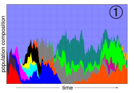
(a)

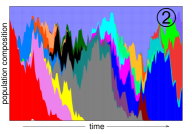
(b)

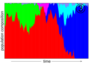
(c)

Figure 4: Mutant frequencies vs. time for the model in section II. Different colors identify different mutants, and blue mesh includes all types that never reach 10% of the total population size. In (c), the population at almost all times is dominated by a single mutant, whose identity is replaced on rapid, successive sweeps. Detailed-balance is known to hold here. In (a+b) more complex patterns are observed. Here too, as we show below (section II), detailed-balance holds, provided that proper averaging on short-times is applied. The labels of the figures help locating them on the phase diagram of Fig 8.

IV.1 The thermal correspondence at low mutation rate

Let us first discuss the line $1/\tau=0$. In this regime, mutations are very rarely proposed, and the system eventually falls in the successional regime ($N/\left(\lambda\tau\right)\ll 1$). As we have seen above, detailed balance is then expected to hold with temperature $T=\frac{L}{N}$. Indeed, in Fig. 5 we show the results of a simulated annealing performed with an ordinary Monte Carlo program on a single sample, superposed with a ‘populational annealing’ performed by slowly increasing the population of a set of individuals performing diffusion and reproducing according to the fitness in Eq. (1). The coincidence of both curves in terms of $T=L/N$ is reassuring.

We note in passing that the ‘thermal’ analysis allows one to make an evaluation of ‘genetic algorithms’ – in this case we understand that the Darwinian Annealing will have the same strengths and weaknesses as has Simulated Annealing. Furthermore, we see that allowing for large populations from the outset may be as catastrophic as is a sudden quench in an annealing procedure.

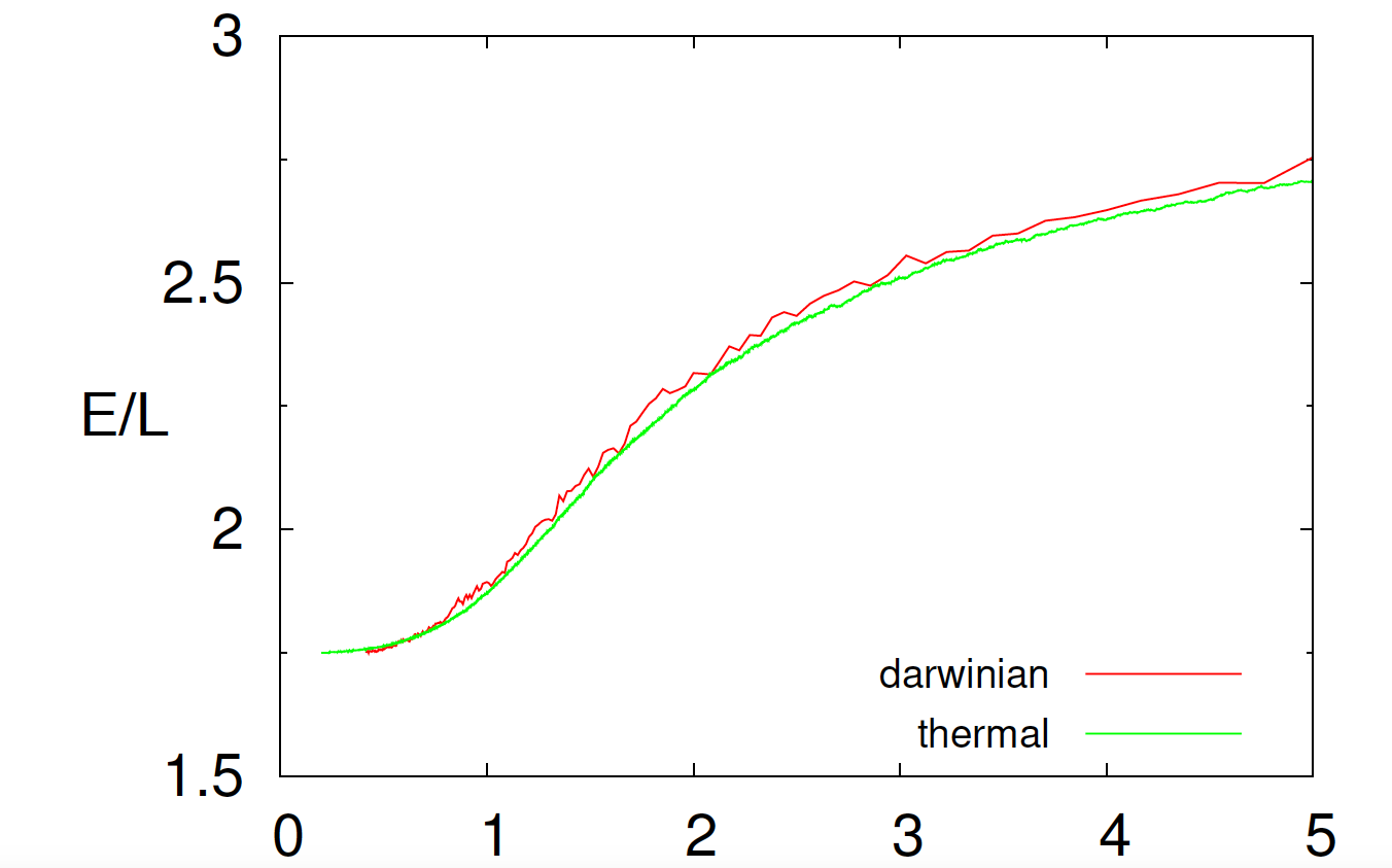
Figure 5: Thermal versus Darwinian annealing for XorSAT, for $\tau=16$. Similar results are obtained for K-SAT. Darwinian annealing is performed by controlling the population so that it increases slowly, at the same rate as in the corresponding thermal annealing with $T=L/N$.

In the limit $\tau\rightarrow\infty$, when the population behaves like a thermal realization of a SAT system at temperature $T=\frac{L}{N}$, the situation is well understood for the XorSAT and the SAT problems krzakala_gibbs_2007 : there is a (dynamic) glass transition at a certain temperature $T_{d}$ below which the phase-space breaks into components, and the dynamics become slow, rendering the optimization very hard. This transition happens before the thermodynamic one, which itself is closely analogous to the freezing one of the REM.

We may locate the dynamic transition by plotting the autocorrelation functions $C(t,t^{\prime})=\frac{4}{L}\sum_{i}(s_{i}\left(t\right)-\frac{1}{2})(s_{i}\left(t^{\prime}\right)-\frac{1}{2})$ at decreasing temperatures. As $T_{d}$ is approached from above, the correlation decays in a two-time process, a fast relaxation to a plateau followed by a much slower ‘$\alpha$-relaxation’ (in the glass terminology), taking a time $t_{\alpha}$. As $T_{d}$ is reached, $t_{\alpha}$ diverges. Below $T_{d}$, the system ages: the time $t_{\alpha}$ now keeps increasing with time, $C(t,t^{\prime})$ decays in a time $(t-t^{\prime})_{decay}\sim t_{\alpha}(t^{\prime})$ with $t_{\alpha}(t^{\prime})$ an increasing function of $t^{\prime}$. What we have described is the ‘Random First Order Transition’ kirkpatrick_scaling_1989 . Nothing new here, as the system is equivalent to a thermal system, known to exhibit such a transition.

Let us now consider smaller $\tau$, so that we no longer can assure that the $N$ individuals are fully clustered in a configuration at most times, and $N$ no longer has an obvious thermal meaning. We approach the transition by increasing $N$ at fixed $\tau$, and also by decreasing $\tau$ at fixed $N$. The correlation curves obtained are shown in Fig (6): the nature of the transition remains the same, but the transition value of critical $N$ shifts with $\tau$. All in all, we obtain NS the phase diagram of Fig 8.

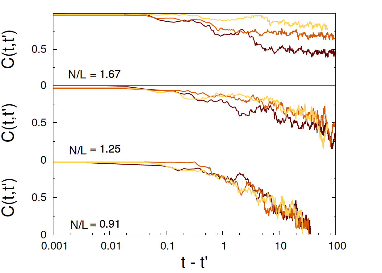
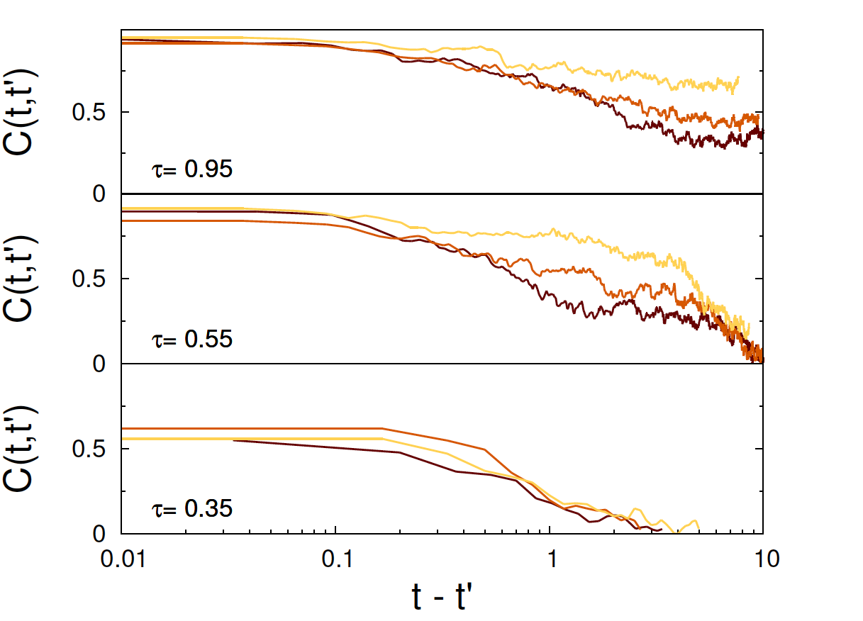
Figure 6: Values of the $C(t,t^{\prime})$ for a population crossing the glass transition from liquid (bottom) to glass (top). Values are $\tau=5$, $N/L={0.91,1.25,1.67}$ (left), and $N/L=4$, $\tau={0.35,0.55,0.95}$. The transition line is thus crossed by increasing $N$ or $\tau$, see the two arrows in fig. 8, the points corresponding to the figures are marked by crosses. The color code indicate the value of $\ln(t^{\prime})$, growing linearly from darker to lighter curves. In the top figures $t_{\alpha}$ grows as the system ages. Here and in all the following figures, the time is measured in units of mutation times $\tau$ (i.e. an individual performs on average $O(L)$ flips in $\Delta t=O\left(1\right)$). The correlations are reasonably smooth, for a big system, even for a single run

A confirmation of this is obtained by plotting the autocorrelation ‘noise’ (also known as dynamic heterogeneity)

$$\chi_{4}=L\left\langle\left[\frac{4}{L}\sum_{i}(s_{i}\left(t\right)-\frac{1}{2})(s_{i}\left(t^{\prime}\right)-\frac{1}{2})\right]^{2}\right\rangle-LC(t,t^{\prime})^{2}$$ (8)

a quantity that peaks at a level expected to diverge at the transition, at a time that we may estimate as $t_{\alpha}$, see Fig 7.

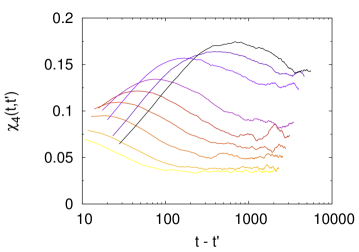
Figure 7: $\chi_{4}$ versus time on approaching the transition. Data shown for $N/L=1.4$, and a mutation rate $\tau^{-1}$ increasing linearly from 0.25 to 0.65 (bottom to top, dark to light curves). At lower mutations rates (not plotted) the glassy phase is reached, and the curves do not present any maximum and keep increasing with the waiting time $t$, as $t_{\alpha}$ is no longer defined.

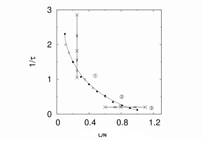
Figure 8: Phase transition diagram in the $L/N$ vs $1/\tau$ plane. The transition line is given by the black circles, which correspond to the points where the value of the maximum in the $\chi_{4}$ function diverges, approaching the line by changing $N$ (filled circles) or $\tau$ (empty circles). The two arrows correspond to two possible crossing of the transition line, changing $\tau$ or $N$, the points indicated by a cross being those represented in Fig 6. Points labeled by numbers correspond to the situations of Fig 4, and indicate the parameters used in the verification of the averaged detailed balance, Fig 9.

Thermal properties of slow dynamics in the region with slow dynamics (large $t_{\alpha}$).

We know that the $\tau^{-1}=0$ axis is just equivalent to the thermal problem, with temperature $L/N$. What can we say about clustering for smaller $\tau$? Figure 4 shows the contributions of different configurations (the top uniform color corresponds to contributions smaller than 10% each). We see that for all but the highest $\tau$, the system is in the concurrent mutation regime desai_beneficial_2007 , and the thermal correspondence, applied naively, breaks down. Considering several examples with timescale separation, we have conjectured unpublished that whenever the $\alpha$ relaxation time is large (near and below the transition), the correspondence with a thermal system may still hold, but taken for quantities that are averaged over a time of several $t_{\alpha}$, and considering two situations at time-separations much larger than $t_{\alpha}$.

Checking detailed balance numerically is extremely hard. We use here a Fluctuation Relation mustonen_fitness_2010 ; evans_fluctuation_2002 , as an indirect test. Because this theorem requires to start from equilibrium, we are only in a position to do the test close to the glass transition, where the time-separation is large enough, but not within, because then equilibration becomes problematic. We thus place ourselves just above the transition (so that a stationary distribution might be reached) but not far from it (so that $t_{\alpha}$ is large), the circled numbers in Figure 8. We start with a system in equilibrium at time $t=0$, and we switch on a field $E\to E-hA$, where $A$ is any observable, in our case we choose $A=\sum_{i}s_{i}$. After an arbitrary time $t$ we measure again the value of $A$ and check the equation (see unpublished )

$$\ln{P[A(t)-A(0)=\Delta]}-\ln{P[A(t)-A(0)=-\Delta]}=\beta h\Delta$$ (9)

We obtain the plot Fig 9 (left). It does not verify the Fluctuation Theorem (9), thus showing that there is no detailed balance or equilibrium, except for very large $\tau$. This is what we expected, as there is no clustering into a single type, and the connection with a thermal system fails. Instead, when we compute the differences as $\Delta=\bar{A}(t)-\bar{A}(t=0)$, with $\bar{A}$ the average of $A$ within a window comparable to the time to reach a plateau – the ‘equilibration within a valley’ time $\ll t_{\alpha}$ – and $t\sim 3t_{\alpha}$, the relation (9) for the averaged values $\Delta=\bar{A}(t)-\bar{A}(0)$ works perfectly, without fitting parameters. We interpret this as meaning that the jumps between valleys, taking a long time, are indeed governed by a temperature $L/N$, although the diffusion inside a valley is not.

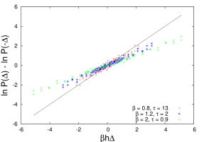
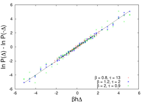
Figure 9: $\ln P(\Delta)-\ln P(-\Delta)$ versus $\beta h\Delta$, for close times and instantaneous values (left) and for quantities averaged over a time-window, and times separated by more than $t_{\alpha}$ (right). The latter works perfectly, without any fitting parameters. The parameters for the three curves, $(\beta,\tau)={(0.8,13),(1.2,2),(2,0.9)}$, correspond to those of figure 4, and are represented on the phase diagram of figure 8.

IV.2 An analogy with dense active matter

Active matter is composed by particles that have a source of energy other than a simple thermal bath. This may be the case of bacteria, of specially defined propulsed particles, and of randomly shaken particles. A way to model this situation, is to consider a source of energy in the high frequencies (for example a thermal bath at high temperature $T_{fast}$ with white noise) and a mechanism of dissipation, such as a thermal bath with low-frequency correlated noise at a lower temperature $T_{slow}$ (see Ref. berthier_non-equilibrium_2013 ). The high frequency source need not be a true thermal bath, it could consist for example of random ‘kicks’. In any case, the system is not truly in equilibrium, because for this one needs a same temperature at all timescales. If one considers a situation with high density and a suitable energy balance situation, the particle system approaches a glass transition just as an ordinary thermal one. Timescale-separation appears, the fast motion is essentially ruled by the ‘fast’ excitation, while the slow motion by the ‘slow’ bath. One expects then detailed balance at temperature $T_{slow}$ to hold for slow evolution and time-averaged quantities, while it does not hold inside a state. The situation is quite close to the one discussed in this paper, the role of the ‘fast’ excitation being played here by the fluctuations due to the Darwinian nature of the dynamics within a state. The parameter $1/\tau$ plays the role of the input energy rate at high frequencies, while $\frac{L}{N}$ plays the role of $T_{slow}$. Our phase diagram Fig. 8 is strikingly similar the one of the active matter model in Ref berthier_non-equilibrium_2013 .

IV.3 Changing environments: connection to glassy rheology

A system as the one we are considering, which is achieving better fitness by slowly adapting to a complex landscape, is extremely sensitive to changes in this landscape. This effect has been discussed in mustonen_molecular_2008 , although in a slightly different form, and also in kussell_phenotypic_2005 . The counterpart in glass physics of this fact has long been known. Consider the situation struik_rejuvenation_1997 of a plastic bar prepared a time $t_{w}$ ago from a melt. The polymers constituting the bar slowly rearrange – ever more slowly – to energetically better and better configurations, and this process is known to go on at least for decades. The bar is out of equilibrium, a fact that we may recognize by testing its response to stress, which measurably depends on $t_{w}$. Now suppose that we apply a large, fixed deformation to the bar, for example applying a strong torsion one way and the other. The new constraints change the problem of optimization the polymers are ‘solving’: we expect evolution to restart to a certain extent, and the apparent ‘age’ of the bar to become smaller than $t_{w}$. This is indeed what happens struik_rejuvenation_1997 , a phenomenon called ‘rejuvenation’. Rejuvenation brings about an acceleration in the dynamics. If the changes are continuous and different, instead of aging (growth of $t_{\alpha}$), the system settles in a value of $t_{\alpha}$ that depends on – adapts to – the speed of change of the energy landscape. Note that this property of evolution speed, as measured from the changes in the population adapting to landscape change speed, that is sometimes attributed to a form of criticality kauffman_metabolic_1969 , here appears as a universal property of aging systems.

Applying the same logic to our model, one expects a similar result. In order to model the changes in fitness landscape, we change at fixed intervals of time a randomly chosen clause, for example by changing the identity of one of the intervening Boolean variables (a slight change in the fitness function). For different rates of change, we plot the ‘age’ of the system, as measured by $\chi_{4}$. The results are shown on Figure 10: if the environment is randomly changing, the system evolves to accommodate various conditions, and time-scales for changes in the environment are reflected in the time-scales for changes inside system.

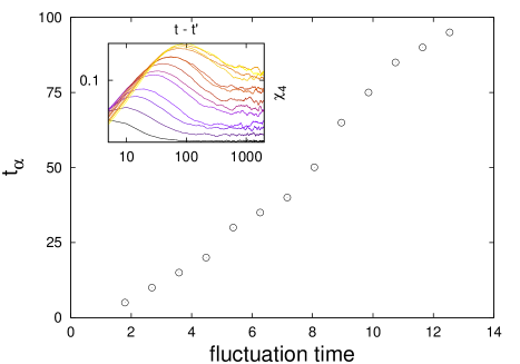
Figure 10: $\alpha$-time versus speed of variation of fitness landscape. Inset: $\chi_{4}$ versus time for different speeds of random variation of landscape (darker curves correspond to faster variations). The $t_{\alpha}$ value for each point of the main figure is the time at which the corresponding curve reaches its maximum, a measure of the $\alpha$-time.

V Conclusions

We have studied the dynamics of a population of random walkers reproducing with a rate corresponding to a ‘rugged’ fitness function. The natural phase variables are the size of the system and the diffusion constant (the mutation rate). We obtain a glassy region in this phase diagram where the systems ‘ages’, slowly evolving to ever better fitnesses. We have found evidence that even for relatively high diffusion constants, the size of the system may be interpreted as an inverse temperature, provided one considers time-averaged quantities. The phase diagram bears a striking resemblance to the one that would be obtained for the same system in contact with a bath at temperature $T$ driven simultaneously at the high frequencies, the intensity of the latter playing the role of the inverse mutation rate $1/\tau$.

- (1) Kirkpatrick, Scott, and Mario P. Vecchi. ”Optimization by simmulated annealing.” science 220.4598 (1983): 671-680; Kirkpatrick, Scott. ”Optimization by simulated annealing: Quantitative studies.” Journal of statistical physics 34.5-6 (1984): 975-986.
- (2) This phase diagram seem very similar to the one obtained by Neher and Shraiman, where recombination and epistasis play the roles of mutation and selection. See: Neher, Richard A., and Boris I. Shraiman. ”Competition between recombination and epistasis can cause a transition from allele to genotype selection.” Proceedings of the National Academy of Sciences 106.16 (2009): 6866-6871.
- (3) Mitchell, Melanie. An introduction to genetic algorithms. MIT press, 1998.
- (4) J. F. Crow and M. Kimura, “An introduction to population genetics theory,” pp. xiv+591 pp., 1970.
- (5) S. Franz, L. Peliti, and M. Sellitto, “An evolutionary version of the random energy model,” J. Phys. A: Math. Gen., vol. 26, no. 23, p. L1195, Dec. 1993.
- (6) Anderson, James B. ”Quantum chemistry by random walk. H 2P, H+ 3D3h1A? 1, H23?+ u, H41?+ g, Be 1S.” The Journal of Chemical Physics 65.10 (1976): 4121-4127.
- (7) Giardina, Cristian, et al. ”Simulating rare events in dynamical processes.” Journal of statistical physics 145.4 (2011): 787-811.
- (8) Eigen, Manfred, John McCaskill, and Peter Schuster. ”The molecular quasi-species.” Adv. Chem. Phys 75 (1989): 149-263.
- (9) L. Peliti, “Introduction to the statistical theory of Darwinian evolution,” arXiv:cond-mat/9712027, Dec. 1997, arXiv: cond-mat/9712027.
- (10) L. S. Tsimring, H. Levine, and D. A. Kessler, “RNA virus evolution via a fitness-space model,” Physical review letters, vol. 76, no. 23, p. 4440, 1996.
- (11) M. Lynch,The Lower Bound to the Evolution of Mutation Rates,” Genome Biol Evol, vol. 3, pp. 1107–1118, Jan. 2011.
- (12) Iwasa, Yoh, Franziska Michor, and Martin A. Nowak. ”Stochastic tunnels in evolutionary dynamics.” Genetics 166.3 (2004): 1571-1579.
- (13) Weissman, Daniel B., et al. ”The rate at which asexual populations cross fitness valleys.” Theoretical population biology 75.4 (2009): 286-300.
- (14) R. A. Neher, M. Vucelja, M. Mezard, and B. I. Shraiman, “Emergence of clones in sexual populations,” Journal of Statistical Mechanics: Theory and Experiment, vol. 2013, no. 01, p. P01008, Jan. 2013.
- (15) G. Sella and A. E. Hirsh, “The application of statistical physics to evolutionary biology,” PNAS, vol. 102, no. 27, pp. 9541–9546, Jul. 2005.
- (16) V. Mustonen and M. Lassig, “Fitness flux and ubiquity of adaptive evolution,” PNAS, vol. 107, no. 9, pp. 4248–4253, Mar. 2010.
- (17) J. Berg and M. Lassig, “Stochastic evolution of transcription factor binding sites,” Biophysics, vol. 48, no. 1, pp. 36–44, 2003.
- (18) J. Berg, S. Willmann, and M. Lassig, “Adaptive evolution of transcription factor binding sites,” BMC Evolutionary Biology, vol. 4, no. 1, p. 42, Oct. 2004.
- (19) N. H. Barton and J. B. Coe, “On the application of statistical physics to evolutionary biology,” Journal of Theoretical Biology, vol. 259, no. 2, pp. 317–324, Jul. 2009.
- (20) P. A. P. Moran, The Statistical Processes of Evolutionary Theory. Clarendon Press, 1962.
- (21) M. A. Nowak, Evolutionary Dynamics. Harvard University Press, Sep. 2006.
- (22) T Brotto, G Bunin and J Kurchan, arXiv:1507.07453 (unpublished).
- (23) M. M. Desai and D. S. Fisher, “Beneficial Mutation-Selection Balance and the Effect of Linkage on Positive Selection,” Genetics, vol. 176, no. 3, pp. 1759–1798, Jul. 2007.
- (24) I. M. Rouzine, J. Wakeley, and J. M. Coffin, “The solitary wave of asexual evolution,” PNAS, vol. 100, no. 2, pp. 587–592, Jan. 2003.
- (25) I. M. Rouzine, Ã. Brunet, and C. O. Wilke, “The traveling-wave approach to asexual evolution: Muller’s ratchet and speed of adaptation,” Theoretical Population Biology, vol. 73, no. 1, pp. 24–46, Feb. 2008.
- (26) Schuster, Peter, and Karl Sigmund. ”Replicator dynamics.” Journal of theoretical biology 100.3 (1983): 533-538.
- (27) B. H. Good, I. M. Rouzine, D. J. Balick, O. Hallatschek, and M. M. Desai, “Distribution of fixed beneficial mutations and the rate of adaptation in asexual populations,” PNAS, vol. 109, no. 13, pp. 4950–4955, Mar. 2012.
- (28) V. Mustonen and M. Lassig, “Molecular Evolution under Fitness Fluctuations,” Physical Review Letters, vol. 100, no. 10, Mar. 2008.
- (29) Kingman, J. F. C. ”A simple model for the balance between selection and mutation.” Journal of Applied Probability (1978): 1-12.
- (30) B. Derrida, “Random-Energy Model: Limit of a Family of Disordered Models,” Phys. Rev. Lett., vol. 45, no. 2, pp. 79–82, Jul. 1980.
- (31) C. Cammarota and E. Marinari, “Spontaneous energy-barrier formation in an entropy-driven glassy dynamics,” arXiv:1410.2116 [cond-mat], Oct. 2014, arXiv: 1410.2116.
- (32) D. A. Kessler, H. Levine, D. Ridgway, and L. Tsimring, “Evolution on a smooth landscape,” J Stat Phys, vol. 87, no. 3-4, pp. 519–544, May 1997.
- (33) Y.-C. Zhang, M. Serva, and M. Polikarpov, “Diffusion reproduction processes,” J Stat Phys, vol. 58, no. 5-6, pp. 849–861, Mar. 1990.
- (34) M. Meyer, S. Havlin, and A. Bunde, “Clustering of independently diffusing individuals by birth and death processes,” Phys. Rev. E, vol. 54, no. 5, pp. 5567–5570, Nov. 1996.
- (35) J. B. Pedersen and P. Sibani, “The long time behavior of the rate of recombination,” The Journal of Chemical Physics, vol. 75, no. 11, pp. 5368–5372, Dec. 1981.
- (36) P. Sibani and A. Pedersen, “Evolution dynamics in terraced NK landscapes,” EPL, vol. 48, no. 3, p. 346, Nov. 1999.
- (37) S. Seetharaman and K. Jain, “Evolutionary dynamics on strongly correlated fitness landscapes,” Phys. Rev. E, vol. 82, no. 3, p. 031109, Sep. 2010.
- (38) D. Saakian and C.-K. Hu, “Eigen model as a quantum spin chain: Exact dynamics,” Phys. Rev. E, vol. 69, no. 2, p. 021913, Feb. 2004.
- (39) D. B. Saakian and J. F. Fontanari, “Evolutionary dynamics on rugged fitness landscapes: Exact dynamics and information theoretical aspects,” Physical Review E, vol. 80, no. 4, Oct. 2009.
- (40) D. B. Saakian and C.-K. Hu, “Solvable biological evolution model with a parallel mutation-selection scheme,” Phys. Rev. E, vol. 69, no. 4, p. 046121, Apr. 2004.
- (41) S. A. Kauffman, “Metabolic stability and epigenesis in randomly constructed genetic nets,” Journal of Theoretical Biology, vol. 22, no. 3, pp. 437–467, Mar. 1969.
- (42) D. Ridgway, H. Levine, and D. A. Kessler, “Evolution on a Smooth Landscape: The Role of Bias,” Journal of Statistical Physics, vol. 90, no. 1-2, pp. 191–210, Jan. 1998.
- (43) F. Krzakala, A. Montanari, F. Ricci-Tersenghi, G. Semerjian, and L. Zdeborova, “Gibbs states and the set of solutions of random constraint satisfaction problems,” PNAS, vol. 104, no. 25, pp. 10 318–10 323, Jun. 2007.
- (44) T. R. Kirkpatrick, D. Thirumalai, and P. G. Wolynes, “Scaling concepts for the dynamics of viscous liquids near an ideal glassy state,” Physical Review A, vol. 40, no. 2, p. 1045, 1989.
- (45) D. J. Evans and D. J. Searles, “The Fluctuation Theorem,” Advances in Physics, vol. 51, no. 7, pp. 1529–1585, Nov. 2002.
- (46) E. Kussell and S. Leibler, “Phenotypic Diversity, Population Growth, and Information in Fluctuating Environments,” Science, vol. 309, no. 5743, pp. 2075–2078, Sep. 2005.
- (47) L. C. E. Struik, “On the rejuvenation of physically aged polymers by mechanical deformation,” Polymer, vol. 38, no. 16, pp. 4053–4057, Aug. 1997.
- (48) Berthier, Ludovic, and Jorge Kurchan. ”Non-equilibrium glass transitions in driven and active matter.” Nature Physics 9.5 (2013): 310-314.