A New Perspective on Randomized Gossip Algorithms

Abstract

In this short note we propose a new approach for the design and analysis of randomized gossip algorithms which can be used to solve the average consensus problem. We show how that Randomized Block Kaczmarz (RBK) method—a method for solving linear systems—works as gossip algorithm when applied to a special system encoding the underlying network. The famous pairwise gossip algorithm arises as a special case. Subsequently, we reveal a hidden duality of randomized gossip algorithms, with the dual iterative process maintaining a set of numbers attached to the edges as opposed to nodes of the network. We prove that RBK obtains a superlinear speedup in the size of the block, and demonstrate this effect through experiments.

Index Terms—  Average Consensus Problem, Linear Systems, Networks, Randomized Gossip Algorithms, Randomized Block Kaczmarz

1 Introduction

The average consensus problem and randomized gossip algorithms for solving it appear in many applications, including distributed data fusion in sensor networks [1], load balancing [2] and clock synchronization [3]. This subject was studied extensively in the last decade; for instance, the seminal 2006 paper of Boyd et al. [4] on randomized gossip algorithms motivated a fury of subsequent research and generated more than 1500 citations to date. For a survey of selected relevant work prior to 2010, we refer the reader to the work of Dimakis et al. [5]. For more recent results on randomized gossip algorithms we suggest [6, 7, 8]. See also [9, 10, 11].

1.1 The average consensus problem

In the average consensus (AC) problem, we are given an undirected connected network $\mathcal{G}=(\mathcal{V},\mathcal{E})$ with node set $\mathcal{V}=\{1,2,\dots,n\}$ and edges $\mathcal{E}$. Each node $i\in\mathcal{V}$ “knows” a private value $c_{i}\in\mathcal{R}$. The goal of AC is for every node of the network to compute the average of these private values, $\bar{c}:=\tfrac{1}{n}\sum_{i}c_{i}$, in a distributed fashion. That is, the exchange of information can only occur between connected nodes (neighbors).

1.2 Contributions

In this paper we revisit, from a fresh perspective, the AC problem. Our starting point is the recent observation of Gower and Richtárik [12] that the most basic randomized gossip algorithm (“randomly pick an edge $(i,j)\in\mathcal{E}$ and then replace the values stored at vertices $i$ and $j$ by their average”) is an instance of the randomized Kaczmarz (RK) method for solving consistent linear systems, applied to a specific linear system encoding the AC problem. The RK method was first analyzed in 2009 by Strohmer and Vershynin [13], and since then, there was an explosion of activity in refining, generalizing and extending the results [14, 15, 16, 17, 18]. In this paper, we examine the Stochastic Dual Ascent (SDA) method of Gower and Richtárik [12], which includes the RK method as a special case, in the context of AC problem. We show how the complexity result of SDA implies a bound on the $\varepsilon$-averaging time which is well-known in the literature for a more restricted class of randomized gossip algorithms. Further, we explain how SDA uncovers a fundamental but hitherto hidden duality of randomized gossip algorithms, and give a natural interpretation thereof. We then focus on a specific subclass of SDA which is identical to the randomized block Kaczmarz method [14] in the primal space, and which can be interpreted as a randomized Newton method in the dual space. In particular, we show that the method has a certain superlinear speedup property, and explain what this property means. Finally, we perform experiments to justify the last claim.

2 SDA: Stochastic Dual Ascent

In this section we briefly review those aspects of the work of Gower and Richtárik [12] on Stochastic Dual Ascent (SDA) which we will need in the rest of the paper.

Consider an $m\times n$ real matrix $\mathbf{A}$ (assume it does not contain any zero rows) and vector $b\in\mathcal{R}^{m}$ such that the linear system $\mathbf{A}x=b$ is consistent (i.e., has a solution). Since we do not assume the solution is unique, we shall be interested in a particular solution:

$$\min_{x=(x_{1},\dots,x_{n})\in\mathcal{R}^{n}}\tfrac{1}{2}\|x-c\|^{2}\quad\text{subject to}\quad\mathbf{A}x=b.$$ (1)

Above, $c=(c_{1},\dots,c_{n})\in\mathcal{R}^{n}$ is a given vector and $\|\cdot\|$ is the standard Euclidean norm. In words, in (1) we are seeking the solution of the system which is closest to $c$. By $x^{*}$ we denote the solution of (1). The dual of problem (1) is

$$\max_{y\in\mathcal{R}^{m}}D(y):=(b-\mathbf{A}c)^{\top}y-\tfrac{1}{2}\|\mathbf{A}^{\top}y\|^{2}.$$ (2)

SDA is a randomized iterative algorithm for solving (2), performing the iteration $y^{k+1}=y^{k}+\mathbf{S}_{k}\lambda^{k}$, where $\mathbf{S}_{k}$ is a matrix chosen in an i.i.d. fashion throughout the iterative process from an arbitrary but fixed distribution (which is a parameter of the method) and $\lambda^{k}$ is a vector chosen afterwards so that $D(y^{k}+\mathbf{S}_{k}\lambda)$ is maximized in $\lambda$. In general, the maximizer in $\lambda$ is not unique. In SDA, we let $\lambda^{k}$ to be the least-norm maximizer, which leads to the iteration

$$\boxed{y^{k+1}=y^{k}-\mathbf{R}_{k}(\mathbf{A}(c+\mathbf{A}^{\top}y^{k})-b)}$$ (3)

where $\mathbf{R}_{k}:=\mathbf{S}_{k}((\mathbf{S}_{k})^{\top}\mathbf{A}\mathbf{A}^{\top}\mathbf{S}_{k})^{\dagger}(\mathbf{S}_{k})^{\top}$ (this matrix is always symmetric and positive semidefinite). With the sequence of the dual iterates $\{y^{k}\}$ we associate a sequence of primal iterates $\{x^{k}\}$ as follows:

$$x^{k}:=c+\mathbf{A}^{\top}y^{k}.$$ (4)

By combining (4) with (3), we obtain the following algorithm:

$$\boxed{x^{k+1}=x^{k}-\mathbf{A}^{\top}\mathbf{R}_{k}(\mathbf{A}x^{k}-b)}$$ (5)

If $\mathbf{S}_{k}$ is chosen randomly from the set of unit coordinate/basis vectors in $\mathcal{R}^{m}$, then the dual method (3) is randomized coordinate descent [19, 20], and the corresponding primal method (5) is RK. More generally, if $\mathbf{S}_{k}$ is a random column submatrix of the $m\times m$ identity matrix, the dual method is the randomized Newton method [21], and the corresponding primal method is a block version of RK [14]. We shall describe the more general case in more detail in Section 4.

The basic convergence guarantees for both the primal and the dual iterative processes are presented in the following theorem. We set $y^{0}=0$ so that $x^{0}=c$, which corresponds to the vector of initial private values stored at the nodes.

Theorem 2.1 (Complexity of SDA [12]).

Let $y^{0}=0$ and assume that the matrix $\mathbf{H}:=\mathbb{E}[\mathbf{R}_{k}]$ is well defined and nonsingular. Then the dual iterates $\{y^{k}\}$ of SDA defined in (3) for all $k\geq 0$ satisfy

$$\mathbb{E}[D(y^{*})-D(y^{k})]\leq\rho^{k}(D(y^{*})-D(y^{0})).$$ (6)

Likewise, the corresponding primal iterates, defined in (4) and explicitly written in (5), for all $k\geq 0$ satisfy

$$\mathbb{E}[\|x^{k}-x^{*}\|^{2}]\leq\rho^{k}\|x^{0}-x^{*}\|^{2}.$$ (7)

The convergence rate $\rho$ is given by

$$\rho:=1-\lambda_{\min}^{+}(\mathbf{A}^{\top}\mathbf{H}\mathbf{A})\in(0,1),$$ (8)

where $\lambda_{\min}^{+}(\cdot)$ denotes the minimum nonzero eigenvalue.

3 Randomized Gossip & SDA

We propose that randomized gossip algorithms be viewed as applications of SDA (either in the primal or dual form) to a particular problem of the form (1) (resp. (2)). In particular, we let $c=(c_{1},\dots,c_{n})$ be the initial values stored at the nodes of $\mathcal{G}$, and choose $\mathbf{A}$ and $b$ so that the constraint $\mathbf{A}x=b$ is equivalent to the requirement that $x_{i}=x_{j}$ (the value stored at node $i$ is equal to the value stored at node $j$) for all $(i,j)\in\mathcal{E}$.

Definition 3.1.

We say that $\mathbf{A}x=b$ is an “average consensus (AC) system” when $\mathbf{A}x=b$ iff $x_{i}=x_{j}$ for all $(i,j)\in\mathcal{E}$.

It is easy to see that $\mathbf{A}x=b$ is an AC system precisely when $b=0$ and the nullspace of $\mathbf{A}$ is $\{t1_{n}:t\in\mathcal{R}\}$, where $1_{n}$ is the vector of all ones in $\mathcal{R}^{n}$. Hence, $\mathbf{A}$ has rank $n-1$. Moreover, it is easy to see that for any AC system, the solution of (1) necessarily is $x^{*}=\bar{c}\cdot 1_{n}$ — this is why we singled out AC systems. In this sense, any algorithm for solving (1) will “find” the average $\bar{c}$. However, in order to obtain a distributed algorithm we need to make sure that only “local” (with respect to $\mathcal{G}$) exchange of information is allowed.

3.1 Standard Form and Mass Preservation

Assume that $\mathbf{A}x=b$ is an AC system. Then the primal iterative process (5) can be written in the form

$$x^{k+1}=\mathbf{W}_{k}x^{k},$$ (9)

where $\mathbf{W}_{k}:=\mathbf{I}-\mathbf{A}^{\top}\mathbf{R}_{k}\mathbf{A}$. Eq (9) is the standard form in which randomized gossip algorithms are written. What is new here is that the iteration matrix $\mathbf{W}_{k}$ has a specific structure which guarantees convergence to $x^{*}$ under very weak assumption (see Theorem 2.1). Note that if $y^{0}=0$, then $x^{0}=c$, i.e., the starting primal iterate is the vector of private values (as should be expected from any gossip algorithm).

The primal iterates (5) of SDA enjoy a mass preservation property (the proof follows from (4) in view of $\mathbf{A}1_{n}=0$):

Theorem 3.2 (Mass preservation).

If $\mathbf{A}x=b$ is an AC system, then the primal iterates (5) for all $k\geq 0$ satisfy: $\tfrac{1}{n}\sum_{i=1}^{n}x_{i}^{k}=\bar{c}$.

3.2 $\varepsilon$-Averaging Time

Let $z^{k}:=\|x^{k}-x^{*}\|$. The typical measure of convergence speed employed in the randomized gossip literature, called $\varepsilon$-averaging time and here denoted by $K(\varepsilon)$, represents the smallest time $k$ for which $x^{k}$ gets within $\varepsilon z^{0}$ from $x^{*}$, with probability greater than $1-\varepsilon$, uniformly over all starting values $x^{0}=c$. More formally, we define

$$K(\varepsilon):=\sup_{c\in\mathcal{R}^{n}}\inf\{k\;:\;\mathbb{P}\left(z^{k}>\varepsilon z^{0}\right)\leq\varepsilon\}.$$

This definition differs slightly from the standard one in that we use $z^{0}$ instead of $\|c\|$.

Inequality (7), together with Markov inequality, can be used to give a bound on $K(\varepsilon)$, formalized next:

Theorem 3.3.

Assume $\mathbf{A}x=b$ is an AC system. Let $y^{0}=0$ and assume $\mathbf{H}=\mathbb{E}[\mathbf{R}_{k}]$ is nonsingular. Then for any $0<\varepsilon<1$ we have $K(\epsilon)\leq 3\log(1/\varepsilon)/\log(1/\rho)\leq\tfrac{3}{1-\rho}\log(1/\epsilon),$ where $\rho$ is defined in (8).

It can be shown that under the assumptions of the above theorem, $\mathbf{A}^{\top}\mathbf{H}\mathbf{A}$ only has a single zero eigenvalue, and hence $\lambda_{\min}^{+}(\mathbf{A}^{\top}\mathbf{H}\mathbf{A})$ is the second smallest eigenvalue of $\mathbf{A}^{\top}\mathbf{H}\mathbf{A}$. Thus, $\rho$ is the second largest eigenvalue of $\mathbf{I}-\mathbf{A}^{\top}\mathbf{H}\mathbf{A}=\mathbb{E}[\mathbf{W}_{k}]$. The bound on $K(\varepsilon)$ appearing in Thm 3.3 is often written with $\rho$ replaced by $\lambda_{2}(\mathbb{E}[\mathbf{W}_{k}])$ [4].

4 Block gossip algorithms

In the previous section we highlighted some properties of SDA relevant to the randomized gossip literature, but without interpreting SDA as a gossip, or for that matter, distributed algorithm. In this section we remedy this by focusing on a particular AC system and a particular random matrix $\mathbf{S}_{k}$. By being specific, we will be able to give a natural interpretation of SDA as a gossip algorithm.

In particular, we choose $\mathbf{A}$ to be the $|\mathcal{E}|\times n$ matrix such that $\mathbf{A}x=0$ directly encodes the constraints $x_{i}=x_{j}$ for $(i,j)\in\mathcal{E}$. That is, row $e=(i,j)\in\mathcal{E}$ of matrix $\mathbf{A}$ contains value $1$ in column $i$, value $-1$ in column $j$ (we use an arbitrary but fixed order of nodes defining each edge in order to fix $\mathbf{A}$) and zeros elsewhere.

Next, $\mathbf{S}_{k}$ is selected in each iteration to be a random column submatrix of the $m\times m$ identity matrix corresponding to columns indexed by a random subset of edges $\mathcal{S}_{k}\subseteq\mathcal{E}$. We shall write $\mathbf{S}_{k}=\mathbf{I}_{\mathcal{S}_{k}}$. If $\mathcal{S}_{k}=\{1,2\}$, for instance, then $\mathbf{S}_{k}$ consists of the first and second column of $\mathbf{I}$. For simplicity, from now on we will drop the subscript and write $\mathcal{S}$ instead of $\mathcal{S}_{k}$. This choice means that primal SDA is the randomized block Kaczmarz (RBK) method.

4.1 Randomized Block Kaczmarz as a Gossip Algorithm

In our setup, the primal iterative process (5) has the form:

$$x^{k+1}=x^{k}-\mathbf{A}^{\top}\mathbf{I}_{\mathcal{S}}(\mathbf{I}_{\mathcal{S}}^{\top}\mathbf{A}\mathbf{A}^{\top}\mathbf{I}_{\mathcal{S}})^{\dagger}\mathbf{I}_{\mathcal{S}}^{\top}\mathbf{A}x^{k}.$$ (10)

Algorithm (10) can be shown to be equivalent to the following “sketch and project” iteration (see [22] for additional equivalent viewpoints):

$$x^{k+1}=\underset{x\in\mathcal{R}^{n}}{\operatorname{argmin}}\{\|x-x^{k}\|^{2}\;:\;\mathbf{I}_{\mathcal{S}}^{\top}\mathbf{A}x=0\}$$ (11)

which is a (more general) variant of the RBK method of Needell [14]. More specifically, this method works by projecting the last iterate $x^{k}$ onto the solution set of a row subsystem of $\mathbf{A}x=0$, where the selected rows correspond to a random subset $\mathcal{S}\subseteq\mathcal{E}$ of selected edges.

While (10) (resp. (11)) may seem to be a complicated algebraic (resp. variational) characterization of the method, due to our choice of $\mathbf{A}$ we have the following result which gives a natural interpretation of RBK as a gossip algorithm (see also Figure 1).

Theorem 4.1 (RBK as a Gossip Algorithm).

Consider the AC problem. Then each iteration of RBK (Algorithm (10)) works as follows: 1) Select a random set of edges $\mathcal{S}\subseteq\mathcal{E}$, 2) Form subgraph $\mathcal{G}_{k}$ of $\mathcal{G}$ from the selected edges 3) For each connected component of $\mathcal{G}_{k}$, replace node values with their average.

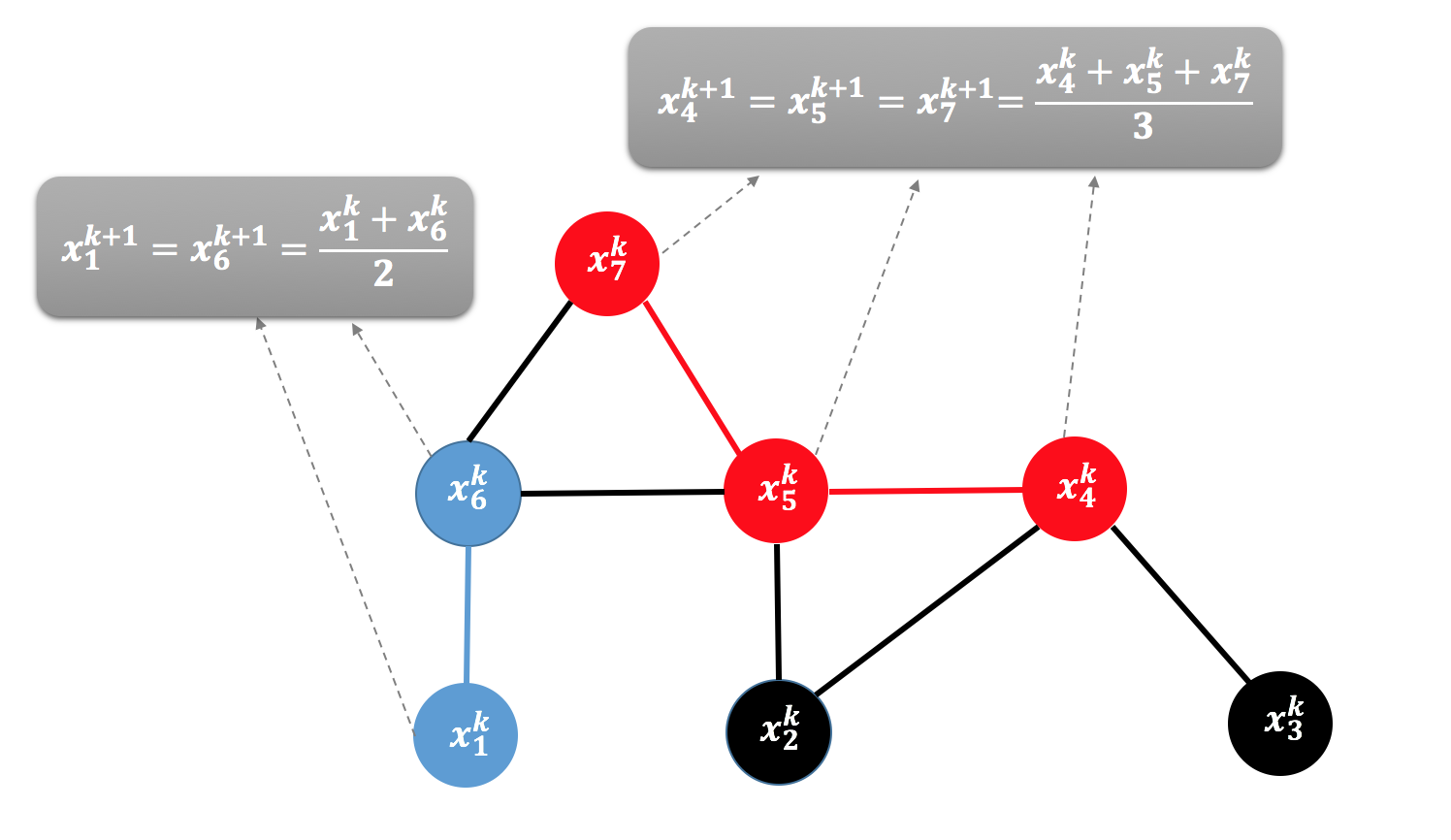
Fig. 1: Example of how the RBK method works as gossip algorithm. In the presented network 3 edges are randomly selected and a subgraph of two connected components (blue and red) is formed. Then the nodes of each connected component update their private values to their average.

There is a very closed relationship between RBK and the path averaging algorithm [23]. The latter is a special case of RBK, when $\mathcal{S}$ is restricted to correspond to a path of vertices. Notice that in the special case in which $\mathcal{S}$ is always a singleton, Algorithm (10) reduces to the randomized Kaczmarz method. This means that only a random edge is selected in each iteration and the nodes incident with this edge replace their local values with their average. This is the pairwise gossip algorithm of Boyd [4]. Theorem 4.1 extends this interpretation to the case of the RBK method.

4.2 Randomized Newton as a Dual Gossip Algorithm

In this subsection we bring a new insight into the randomized gossip framework by presenting how the dual iterative process that is associated to RBK method solves AC problem. The dual iterative process (3) takes on the form:

$$y^{k+1}=y^{k}-\mathbf{I}_{\mathcal{S}}(\mathbf{I}_{\mathcal{S}}^{\top}\mathbf{A}\mathbf{A}^{\top}\mathbf{I}_{\mathcal{S}})^{\dagger}\mathbf{A}(c+\mathbf{A}^{\top}y^{k}).$$ (12)

This is a randomized variant of the Newton method applied to the problem of maximizing the quadratic function $D(y)$ defined in (2). Indeed, as we have seen before, in each iteration we perform the update $y^{k+1}=y^{k}+\mathbf{I}_{\mathcal{S}}\lambda^{k}$, where $\lambda^{k}$ is chosen greedily so that $D(y^{k+1})$ is maximized. In doing so, we invert a random principal submatrix of the Hessian of $D$, whence the name.

Randomized Newton Method (RNM) was first proposed by Qu et al. [21]. RNM was first analyzed as an algorithm for minimizing smooth strongly convex functions. In [12] it was also extended to the case of a smooth but weakly convex quadratics. This method was not previously associated with any gossip algorithm.

The most important distinction of RNM compared to existing gossip algorithms is that it operates with values that are associated to the edges of the network. To the best of our knowledge, it the first randomized dual gossip method. In particular, instead of iterating over values stored at the nodes, RNM uses these values to update “dual weights” $y^{k}\in\mathcal{R}^{m}$ that correspond to the edges $\mathcal{E}$ of the network. However, deterministic dual distributed averaging algorithms were proposed before [24, 25].

Natural Interpretation. In iteration $k$, RNM (Algorithm (12)) executes the following steps: 1) Select a random set of edges $\mathcal{S}_{k}\subseteq\mathcal{E}$, 2) Form a subgraph $\mathcal{G}_{k}$ of $\mathcal{G}$ from the selected edges, 3) The values of the edges in each connected component of $\mathcal{G}_{k}$ are updated: their new values are a linear combination of the private values of the nodes belonging to the connected component and of the adjacent edges of their connected components.

Dual Variables as Advice. The weights $y^{k}$ of the edges have a natural interpretation as advice that each selected node receives from the network in order to update its value (to one that will eventually converge to the desired average).

Consider RNM performing the $k^{th}$ iteration and let $\mathcal{V}_{r}$ denote the set of nodes of the selected connected component that node $i$ belongs to. Then, from Theorem  4.1 we know that $x_{i}^{k+1}=\sum_{i\in\mathcal{V}_{r}}x_{i}^{k}/|\mathcal{V}_{r}|$. Hence, by using (4), we obtain the following identity:

$$\textstyle(\mathbf{A}^{\top}y^{k+1})_{i}=\tfrac{1}{|\mathcal{V}_{r}|}\sum_{i\in\mathcal{V}_{r}}(c_{i}+(\mathbf{A}^{\top}y^{k})_{i})-c_{i}$$ (13)

Thus in each step $(\mathbf{A}^{\top}y^{k+1})_{i}$ represents the term (advice) that must be added to the initial value $c_{i}$ of node $i$ in order to update its value to the average of the values of the nodes of the connected component $i$ belongs to.

4.3 Importance of the dual perspective

It was shown in [21] that when RNM (and as a result, RBK) is viewed as a family of methods indexed by the size $\tau=|\mathcal{S}|$ (we choose $\mathcal{S}$ of fixed size in the experiments), then $\tau\to 1/(1-\rho)$, where $\rho$ is defined in (8), decreases superlinearly fast in $\tau$. In [21], this was only shown for full rank $\mathbf{A}$. In the next result we extend it to AC matrices $\mathbf{A}$ (which are necessarily rank-deficient).

Theorem 4.2.

RBK enjoys superlinear speedup in $\tau$. That is, as $\tau$ increases by some factor, the iteration complexity drops by a factor that is at least as large.

5 Numerical Experiments

We devote this section to experimentally evaluate the performance of the proposed gossip algorithms: RBK (the primal method) and RNM (the dual method). Recall that these methods solve the same problem, and their iterates are related via a simple affine transform. Hence, all results shown apply to both RBK and RNM.

Through these experiments we demonstrate the theoretical results presented in the previous section. That is, we show that for a connected network $\mathcal{G}$, the complexity improves superlinearly in $\tau=|\mathcal{S}|$, where $\mathcal{S}$ is chosen as a subset of $\mathcal{E}$ of size $\tau$, uniformly at random. In comparing the number of iterations for different values of $\tau$, we use the relative error $\varepsilon=\|x^{k}-x^{*}\|/\|c-x^{*}\|$. We let $c_{i}=i$ for each node $i\in\mathcal{V}$. We run RBK until the relative error becomes smaller than $0.01$. The blue solid line in the figures denotes the actual number of iterations (after running the code) needed in order to achieve $\varepsilon\leq 10^{-2}$ for different values of $\tau$. The green dotted line represents the function $f(\tau):=\frac{\ell}{\tau}$, where $\ell$ is the number of iterations of RBK with $\tau=1$ (i.e., the pairwise gossip algorithm). The green line depicts linear speedup; the fact that the blue line (obtained through experiments) is below the green line points to superlinear speedup.

The networks used in our experiments are the ring graph (cycle) with 30 and 100 nodes (Fig 2) and the $4\times 4$ grid graph (Fig 3). When we choose $|\mathcal{S}|=m$ (i.e., we choose to update dual variables corresponding to all edges in each iteration), then $\rho=0$, and thus the method converges in one step.

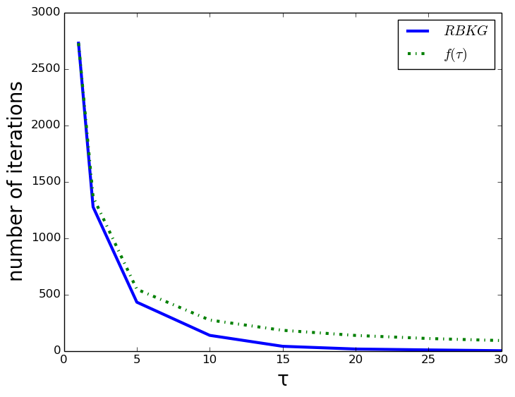
(a) Ring graph with $n=30$

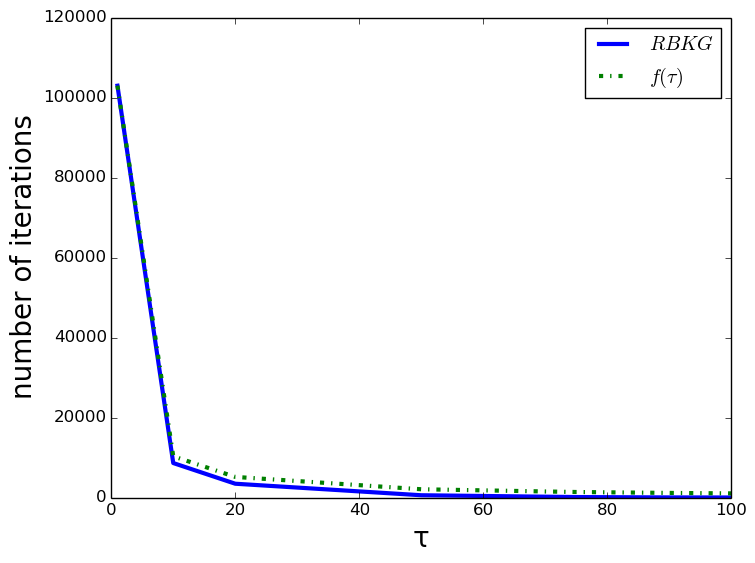
(b) Ring graph with $n=100$

Fig. 2: Superlinear speedup of RBK on the ring graph.

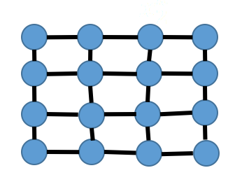
(a) $4\times 4$ grid graph

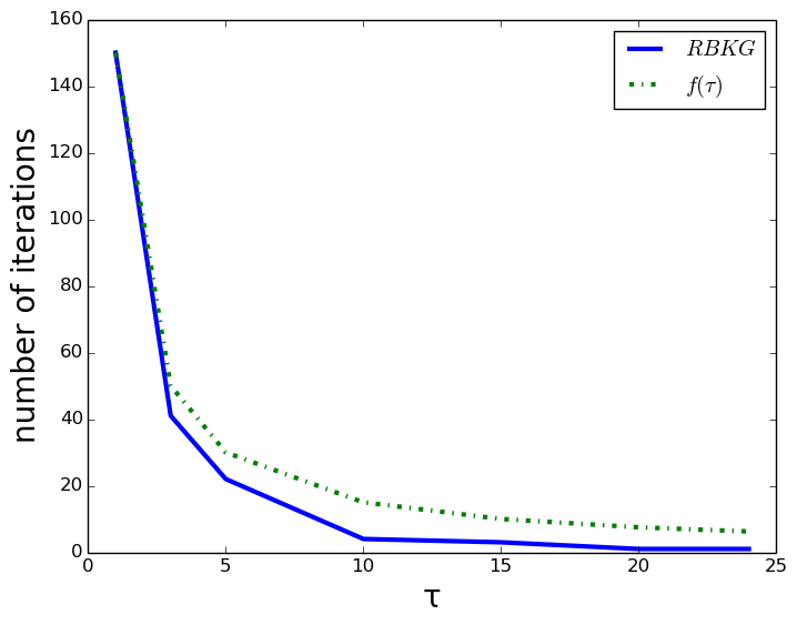
(b) Speedup in $\tau$

Fig. 3: Superlinear speedup of RBK on the $4\times 4$ grid graph

References

- [1] L. Xiao, S. Boyd, and S. Lall, “A scheme for robust distributed sensor fusion based on average consensus,” in Information Processing in Sensor Networks, 2005. IPSN 2005. Fourth International Symposium on. IEEE, 2005, pp. 63–70.
- [2] G. Cybenko, “Dynamic load balancing for distributed memory multiprocessors,” J. Parallel Distrib. Comput., vol. 7, no. 2, pp. 279–301, 1989.
- [3] N.M. Freris and A. Zouzias, “Fast distributed smoothing of relative measurements,” in Decision and Control (CDC), 2012 IEEE 51st Annual Conference on. IEEE, 2012, pp. 1411–1416.
- [4] S. Boyd, A. Ghosh, B. Prabhakar, and D. Shah, “Randomized gossip algorithms,” IEEE Trans. Inf. Theory, vol. 14, no. SI, pp. 2508–2530, 2006.
- [5] A.G. Dimakis, S. Kar, J.M.F. Moura, M.G. Rabbat, and A. Scaglione, “Gossip algorithms for distributed signal processing,” Proceedings of the IEEE, vol. 98, no. 11, pp. 1847–1864, 2010.
- [6] J.Y. Yu and M.G. Rabbat, “Performance comparison of randomized gossip, broadcast gossip and collection tree protocol for distributed averaging,” in Computational Advances in Multi-Sensor Adaptive Processing (CAMSAP), 2013 IEEE 5th International Workshop on. IEEE, 2013, pp. 93–96.
- [7] A. Zouzias and N.M. Freris, “Randomized gossip algorithms for solving Laplacian systems,” in Control Conference (ECC), 2015 European. IEEE, 2015, pp. 1920–1925.
- [8] J. Liu, B.D.O. Anderson, M. Cao, and A.S. Morse, “Analysis of accelerated gossip algorithms,” Automatica, vol. 49, no. 4, pp. 873–883, 2013.
- [9] A.G. Dimakis, A.D. Sarwate, and M.J. Wainwright, “Geographic gossip: Efficient averaging for sensor networks,” IEEE Trans. Signal Process., vol. 56, no. 3, pp. 1205–1216, 2008.
- [10] T.C. Aysal, M.E. Yildiz, A.D. Sarwate, and A. Scaglione, “Broadcast gossip algorithms for consensus,” IEEE Trans. Signal Process., vol. 57, no. 7, pp. 2748–2761, 2009.
- [11] A. Olshevsky and J.N. Tsitsiklis, “Convergence speed in distributed consensus and averaging,” SIAM J. Control Optim., vol. 48, no. 1, pp. 33–55, 2009.
- [12] R.M. Gower and P. Richtárik, “Stochastic dual ascent for solving linear systems,” arXiv preprint arXiv:1512.06890, 2015.
- [13] T. Strohmer and R. Vershynin, “A randomized Kaczmarz algorithm with exponential convergence,” J. Fourier Anal. Appl., vol. 15, no. 2, pp. 262–278, 2009.
- [14] D. Needell and J.A. Tropp, “Paved with good intentions: analysis of a randomized block Kaczmarz method,” Linear Algebra Appl., vol. 441, pp. 199–221, 2014.
- [15] A. Zouzias and N.M. Freris, “Randomized extended Kaczmarz for solving least squares,” SIAM. J. Matrix Anal. & Appl., vol. 34, no. 2, pp. 773–793, 2013.
- [16] Y.C. Eldar and D. Needell, “Acceleration of randomized Kaczmarz method via the Johnson–Lindenstrauss lemma,” Numerical Algorithms, vol. 58, no. 2, pp. 163–177, 2011.
- [17] J. Liu and S. Wright, “An accelerated randomized Kaczmarz algorithm,” Mathematics of Computation, vol. 85, no. 297, pp. 153–178, 2016.
- [18] D. Needell, R. Zhao, and A. Zouzias, “Randomized block Kaczmarz method with projection for solving least squares,” Linear Algebra Appl., vol. 484, pp. 322–343, 2015.
- [19] D. Leventhal and A.S. Lewis, “Randomized methods for linear constraints: convergence rates and conditioning,” Math. Oper. Res., vol. 35, no. 3, pp. 641–654, 2010.
- [20] P. Richtárik and M. Takáč, “Iteration complexity of randomized block-coordinate descent methods for minimizing a composite function,” Math. Program., vol. 144, no. 2, pp. 1–38, 2014.
- [21] Z. Qu, P. Richtárik, M. Takáč, and O. Fercoq, “SDNA: Stochastic dual Newton ascent for empirical risk minimization,” ICML, 2016.
- [22] R.M. Gower and P. Richtárik, “Randomized iterative methods for linear systems,” SIAM. J. Matrix Anal. & Appl., vol. 36, no. 4, pp. 1660–1690, 2015.
- [23] F. Bénézit, A.G. Dimakis, P. Thiran, and M. Vetterli, “Order-optimal consensus through randomized path averaging,” IEEE Trans. Inf. Theory, vol. 56, no. 10, pp. 5150–5167, 2010.
- [24] M.G. Rabbat, R.D. Nowak, and J.A. Bucklew, “Generalized consensus computation in networked systems with erasure links,” in IEEE 6th Workshop on Signal Processing Advances in Wireless Communications. IEEE, 2005, pp. 1088–1092.
- [25] E. Ghadimi, A. Teixeira, M.G. Rabbat, and M. Johansson, “The admm algorithm for distributed averaging: Convergence rates and optimal parameter selection,” in 2014 48th Asilomar Conference on Signals, Systems and Computers. IEEE, 2014, pp. 783–787.