The amplitude mode in three-dimensional dimerized antiferromagnets

Abstract

The amplitude (“Higgs”) mode is a ubiquitous collective excitation related to spontaneous breaking of a continuous symmetry. We combine quantum Monte Carlo (QMC) simulations with stochastic analytic continuation to investigate the dynamics of the amplitude mode in a three-dimensional dimerized quantum spin system. We characterize this mode by calculating the spin and dimer spectral functions on both sides of the quantum critical point, finding that both the energies and the intrinsic widths of the excitations satisfy field-theoretical scaling predictions. While the line width of the spin response is close to that observed in neutron scattering experiments on TlCuCl₃, the dimer response is significantly broader. Our results demonstrate that highly non-trivial dynamical properties are accessible by modern QMC and analytic continuation methods.

The spontaneous breaking of a continuous symmetry allows collective excitations of the direction and amplitude of the order parameter; for O($N$) symmetry, there are $N\!-\!1$ massless directional (Goldstone) modes and one massive amplitude mode Goldstone et al. (1962); Higgs (1964); Zinn-Justin (2002); Sachdev (2011). In loose analogy with the Standard Model, the latter is often called a Higgs mode. A strongly damped amplitude mode has been reported in two dimensions (2D) at the Mott transition of ultracold bosons Endres et al. (2012) and at the disorder-driven superconductor–insulator transition Swanson et al. (2014); Sherman et al. (2015). In 3D, the amplitude mode is expected on theoretical grounds to be more robust, and indeed the cleanest observation to date of a “Higgs boson” in condensed matter is at the pressure-induced magnetic quantum phase transition (QPT) in the dimerized quantum antiferromagnet TlCuCl₃ Rüegg et al. (2004, 2008); Merchant et al. (2014).

Below the upper critical number of space-time dimensions, which for an O($N$) model is $D_{c}=4$, the amplitude mode is unstable, decaying primarily into pairs of Goldstone bosons Sachdev (1999); Zwerger (2004); Dupuis (2011). In both 2D and 3D, the longitudinal dynamic susceptibility exhibits an infrared singularity due to the Goldstone modes Podolsky et al. (2011), whose consequences for the visibility of the amplitude mode have been investigated extensively in 2D Podolsky and Sachdev (2012); Gazit et al. (2013a, b). It was noted Podolsky et al. (2011) that the scalar O($N$)-symmetric susceptibility remains uncontaminated by infrared contributions, which should permit the amplitude mode to be observed as a well-defined peak. The (3+1)D O(3) case of TlCuCl₃ is at $D_{c}$ and the amplitude mode is critically damped, meaning that its width is proportional to its energy at the mean-field level Rüegg et al. (2008); ra ; raw ; Kulik11 . This mode can be probed through the spin response (longitudinal susceptibility) by neutron spectroscopy, and measurements over a wide range of pressures reveal a rather narrow peak width of just 15% of the excitation energy Merchant et al. (2014). The value of this near-constant width-to-energy ratio is the key to the mode visibility, thus calling for unbiased numerical calculations in suitable model Hamiltonians.

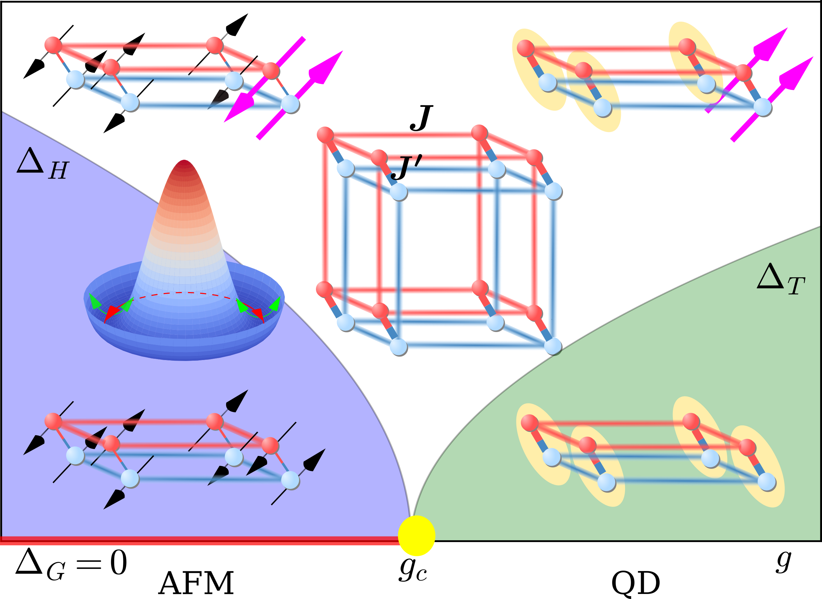
Figure 1: Schematic representation of ground states, excitation processes, and corresponding gaps in a dimerized antiferromagnet. The ratio $g=J^{\prime}/J$ of the intra- and inter-dimer coupling constants controls a QPT from an AFM to a QD state. In the AFM phase, the excitations are two gapless spin waves (Goldstone modes, $\Delta_{G}=0$, red line) plus an amplitude mode with gap $\Delta_{H}$, corresponding respectively to axial and radial fluctuations in the “Mexican hat” potential. In the QD phase, singlet–triplet dimer excitations have gap $\Delta_{T}$.

In this Letter, we provide a systematic investigation of the dynamics and scaling of the amplitude mode at coupling values across the QPT in a 3D dimerized spin-$1/2$ antiferromagnet, by performing large-scale stochastic series expansion quantum Monte Carlo (SSE-QMC) simulations and applying advanced stochastic analytic-continuation (SAC) methods. Thus we provide an unbiased numerical demonstration that the amplitude mode is critically damped and that its energy, width, and height obey field-theoretical predictions. Beyond these universal scaling forms, we quantify the nonuniversal width-to-energy ratios of the amplitude-mode peaks in the spin and dimer channels.

We consider the double-cubic geometry shown in Fig. 1 Jin and Sandvik (2012), which consists of two simple cubic lattices whose sites are connected pairwise by nearest-neighbor Heisenberg exchange interactions, $J_{ij}{\vec{S}}_{i}\!\cdot\!{\vec{S}}_{j}$, with $J_{ij}=J$ in each cubic lattice and $J_{ij}=J^{\prime}$ for inter-cube (dimer) bonds. Increasing the ratio $g\!=\!J^{\prime}/J$ drives a QPT where the ground state changes from a “renormalized classical” rchn ; rcsy antiferromagnetic (AFM) state to a quantum disordered (QD) dimer-singlet state (Fig. 1). This transition is in the same universality class as the pressure-driven QPT in TlCuCl₃. In a recent QMC analysis of the static properties of the double-cubic system Qin et al. (2015), we established the quantum critical point (QCP) as $g_{c}=4.83704(6)$ and quantified the logarithmic (log) scaling corrections expected near criticality in the AFM state at $D_{c}$.

We use SSE-QMC Sandvik (1999); Syljuåsen and Sandvik (2002) to measure both spin and dimer correlation functions in imaginary time; technical details may be found in Sec. SI of the Supplemental Material (SM sm ). The former probes $S=1$ excitations of the ground state and contains the longitudinal susceptibility, while the latter, the symmetric scalar response Podolsky et al. (2011); Podolsky and Sachdev (2012); Gazit et al. (2013a), probes $S=0$ excitations. We employ SAC methods Sandvik (1998); Beach2004 ; Syljuasen2008 ; Fuchs2010 ; Sandvik2015 ; Shao2016 to obtain high-resolution data for the spin and dimer spectral functions, and discuss the concepts and practicalities of this procedure in Sec. SII of the SM sm . Depending on the value of $g$, both spectral functions contain features arising from the Goldstone, amplitude, and triplon (gapped singlet-triplet) excitations. Henceforth we use the term “Higgs” as shorthand for the amplitude-mode contributions. The nature and energies of these modes are represented schematically in Fig. 1.

Our simulations are performed on a system of $N=2L^{3}$ sites at an inverse temperature $J\beta=2L$, such that the low-temperature limit, $T\to 0$, is achieved as $L\to\infty$. The dynamical magnetic ($S=1$) response is obtained from the spin correlation function

$$S(\mathbf{q},\tau)=\langle S^{z}_{-\mathbf{q}}(\tau)S^{z}_{\mathbf{q}}(0)\rangle,$$ (1)

where $\tau$ is the imaginary time [Eq. (S1)] and

$$S^{z}_{\mathbf{q}}=\frac{1}{\sqrt{N}}\mbox{$\sum_{\mathbf{r}}$}{\rm e}^{-i\mathbf{q}\cdot\mathbf{r}}(S^{1z}_{r}-S^{2z}_{r}),$$ (2)

where superscripts 1 and 2 denote the two cubic lattices. When analytically continued to real frequency, $S(\mathbf{q},\tau)$ gives the dynamical structure factor, $S(\mathbf{q},\omega)$, measured by inelastic neutron scattering. Our simulations contain no breaking of spin-rotation symmetry and thus do not separate the longitudinal and transverse components of $S(\mathbf{q},\omega)$ explicitly. The Higgs mode of the AFM phase is contained in the longitudinal part, but the transverse part contains both spin-wave excitations and a multimagnon continuum that could obscure the Higgs contribution in the rotationally averaged $S(\mathbf{q},\omega)$. However, unlike the 2D case Sandvik2001 , the transverse continuum is expected to be very small in 3D, especially at the staggered wave vector, $\mathbf{q}=\mathbf{Q}=(\pi,\pi,\pi)$, on which we focus here.

The scalar ($S=0$) dynamical response is obtained from the dimer correlation function at the zone center, $\mathbf{q}=\mathbf{\Gamma}=(0,0,0)$, which is given by

$$D(\mathbf{\Gamma},\tau)=\langle B_{\mathbf{\Gamma}}(\tau)B_{\mathbf{\Gamma}}(0)\rangle,~{}~{}B_{\mathbf{\Gamma}}=\frac{1}{\sqrt{N}}\sum_{r}B_{r},$$ (3)

where $B_{r}=\mathbf{S}_{r}^{1}\cdot\mathbf{S}_{r}^{2}-\langle\mathbf{S}_{r}^{1}\cdot\mathbf{S}_{r}^{2}\rangle$ is the inter-cubic dimer bond operator. This quantity was also employed in a recent study of the (2+1)D (bilayer) model Lohöfer et al. (2015). The real-frequency quantity $D(\mathbf{\Gamma},\omega)$ may be probed experimentally by Raman scattering Fleury and Loudon (1968); Shastry and Shraiman (1990).

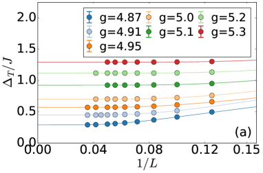
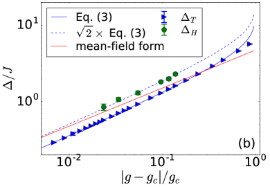
Figure 2: (a) Extrapolation of finite-size triplon gaps, using the form $\Delta_{T}(L)=a\exp(-bL)+c$, shown for selected values of $g>g_{c}$ (QD phase). (b) Triplon gaps in the thermodynamic limit (blue triangles), shown as a function of $|g-g_{c}|/g_{c}$. The red line is a pure mean-field (square-root) form, the blue line includes the log correction of Eq. (4) with fitted exponent $\hat{\nu}=0.230(2)$, and green points show the extrapolated Higgs energy, $\Delta_{H}$, obtained for values of $g<g_{c}$ (AFM phase) mirroring those used in panel (a). The blue dashed line is the log-corrected $\Delta_{T}$ result multiplied by $\sqrt{2}$. Error bars in both panels are smaller than the symbol sizes.

Gap information can also be extracted by a direct analysis of the large-$\tau$ decay of the correlation functions Sen2015 ; Suwa2016 . Considering the spin sector, the smallest singlet-triplet gap occurs at $\mathbf{q}=\mathbf{Q}$ and in the QD phase $S(\mathbf{Q},\tau)$ is dominated by the triplon mode. In the AFM phase, this gap corresponds to the lowest Goldstone mode, which has only a finite-size energy proportional to $1/N$. Thus $S(\mathbf{Q},\tau)$ decays very slowly with $\tau$ in this case and the dominant Goldstone contribution threatens to obscure the Higgs contribution Podolsky et al. (2011); Podolsky and Sachdev (2012); Gazit et al. (2013a, b); Katan and Podolsky (2015). Examples of imaginary-time data for $S(\mathbf{Q},\tau)$ and of gap extractions are presented in Secs. SII and SIII of the SM sm .

We begin the discussion of our results by analyzing the triplon gap in the QD phase ($g>g_{c}$). For a given value of $g$, we extract the finite-size gap, $\Delta_{T}(L)$, from $S(\mathbf{Q},\tau)$ for a range of system sizes. As shown in Fig. 2(a), $\Delta_{T}(L)$ decreases with increasing $L$ before converging to the thermodynamic limit. The extrapolated values of $\Delta_{T}(g)$ are shown in Fig. 2(b) as a function of the separation ($|g-g_{c}|/g_{c}$) from the QCP.

In the $\phi^{4}$ theory for an O($N$) order parameter, at $D=D_{c}$ one expects physical quantities to exhibit power-law scaling with mean-field critical exponents, but with multiplicative log corrections Zinn-Justin (2002); Kenna (2004), which have now been found in a number of recent studies Scammell and Sushkov (2015); Qin et al. (2015); Jiang2016 . The scaling form of the triplon gap can be obtained directly from the correlation length ($\Delta\sim 1/\xi$), whence

$$\Delta_{T}\thicksim(|g-g_{c}|/g_{c})^{\nu}\ln^{-\hat{\nu}}(|g-g_{c}|/g_{c}),$$ (4)

with $\nu=1/2$ Zinn-Justin (2002); sachdev2009exotic and $\hat{\nu}={(N+2)}/{2(N+8)}$ from perturbative renormalization-group calculations Kenna (2004, 2012), i.e. $\hat{\nu}={5}/{22}\approx 0.227$ for $N=3$. It is clear from Fig. 2(b) that Eq. (4) describes the data far better than the pure mean-field form and, by performing an optimized fit (Qin et al., 2015) with $\hat{\nu}$ as a free parameter, we deduce the exponent $\hat{\nu}=0.230(2)$, fully consistent with the theoretical prediction.

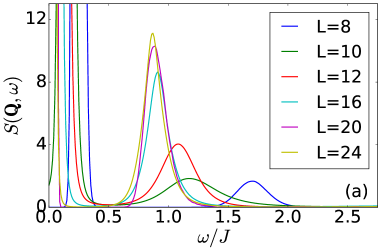
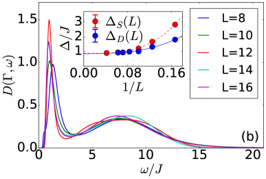
Figure 3: (a) $S(\mathbf{Q},\omega)$ and (b) $D(\mathbf{\Gamma},\omega)$ obtained by SAC at $g=4.724$ for different system sizes. The large low-energy (Goldstone) peak in panel (a) is cut off in order to show the secondary (Higgs) peak. The lower peak in panel (b) is the Higgs mode. The positions of both Higgs contributions converge with increasing $L$ to the same thermodynamic limit, as shown in the inset of panel (b). Spectral features outside the energy ranges shown are extremely weak.

To study the amplitude mode in detail, we analyze the spectral functions $S(\mathbf{Q},\omega)$ and $D(\mathbf{\Gamma},\omega)$ in the AFM phase ($g<g_{c}$) near $g_{c}$. Figure 3 shows both quantities at $g=4.724$ for several system sizes. Because SSE-QMC calculations of $D(\mathbf{\Gamma},\tau)$ are significantly more demanding (Sec. SI), these are restricted to $L\leq 16$, whereas for $S(\mathbf{Q},\tau)$ we access sizes up to $L=24$.

$S(\mathbf{Q},\omega)$ [Fig. 3(a)] is dominated by the Goldstone contribution, whose energy (spectral weight) is proportional to $1/N$ ($N$) at $T=0$ (becoming the magnetic Bragg peak as $L\to\infty$). The Higgs spectral weight also diverges as $g\to g_{c}$; away from $g_{c}$ the Higgs mode remains as a clearly resolved finite-energy peak with convergent spectral weight, as also observed experimentally in TlCuCl₃ Rüegg et al. (2008); Merchant et al. (2014). In $D(\mathbf{\Gamma},\omega)$ [Fig. 3(b)], the Higgs contribution is the distinctive low-energy peak. It is separated by a region of suppressed spectral weight from a broad maximum at higher energies due to multiple excitations. At low energies one expects a characteristic scaling form on which we comment in detail below.

We observe good convergence with increasing $L$ in each of $S(\mathbf{Q},\omega)$ and $D(\mathbf{\Gamma},\omega)$. The peak widths in both quantities are invariant on increasing the amount of QMC data, demonstrating that any artificial broadening arising from the SAC procedure is negligible. Examples of supporting tests are presented in Sec. SII of the SM sm . We have confirmed by a bootstrapping analysis that the fluctuations in the height and width of the lower $D(\mathbf{\Gamma},\tau)$ peak for $L\geq 10$ in Fig. 3(b) reflect statistical errors. Our system sizes are sufficient for a reliable study of the $L\to\infty$ limit in both sectors for the $g$ values shown in Fig. 3 (i.e. $g\approx g_{c}-0.1$).

We find that the positions of the finite-energy peaks in $S(\mathbf{Q},\tau)$ and $D(\mathbf{\Gamma},\tau)$ converge to the same value as $L\to\infty$ [inset, Fig. 3(b)]. In the phenomenological U(1) model for the broken-symmetry phase, one expects the $S=0$ Higgs mode to be an elementary scalar Varma2015 , and thus in the AFM phase that the Higgs part of the $S=1$ spectrum arises from a combination of this scalar with a gapless spin wave ($S=1$, $\mathbf{q}=\pm\mathbf{Q}$). Although our finite-size calculations contain no explicit symmetry-breaking, they reflect this physics directly in that the spin peak lies higher than the dimer peak and their energy difference scales with $1/N$, as expected for a Goldstone mode. Thus the consistency between peaks in the $S=0$ and 1 spectral functions provides strong confirmation that both do indeed correspond to the Higgs mode.

In Fig. 2(b) we compare the extrapolated Higgs energies in the AFM phase with the triplet gaps in the QD phase at the same distance, $|g-g_{c}|/g_{c}$, from the QCP. The predicted $\sqrt{2}$ ratio sachdev2009exotic ; Katan and Podolsky (2015); Scammell and Sushkov (2015) between $\Delta_{H}$ and $\Delta_{T}$ is clearly obeyed over this rather broad coupling range. We stress that this relation implies the presence of equivalent multiplicative log corrections [Eq. (4)] to both $\Delta_{T}$ in the QD phase and $\Delta_{H}$ on the AFM side.

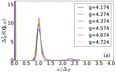
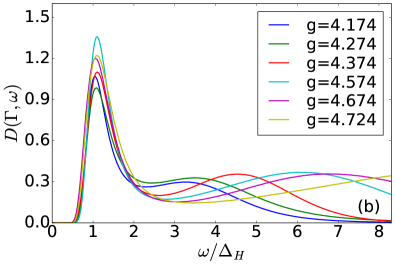
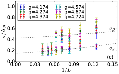
Figure 4: (a) Scaled spectrum, $\Delta_{H}^{2}S(\mathbf{Q},\omega/\Delta_{H})$, calculated with $L=24$ for a range of $g$ values. (b) $D(\mathbf{\Gamma},\omega/\Delta_{H})$ calculated with $L=16$. (c) Width-to-energy ratios shown as functions of $1/L$. Circles and triangles are obtained respectively from $D(\mathbf{\Gamma},\omega/\Delta_{H})$ and $S(\mathbf{Q},\omega/\Delta_{H})$. Dashed lines are second-order polynomial fits to error-weighted average ratios.

To investigate the scaling properties of the spectral functions near the QCP, we normalize $\omega$ by the $L\to\infty$ Higgs gap; results for $\Delta_{H}^{2}S(\mathbf{Q},\omega/\Delta_{H})$ and $D(\mathbf{\Gamma},\omega/\Delta_{H})$ are shown respectively in Figs. 4(a) and 4(b) for the largest accessible system sizes. The amplitude-mode contributions to both the spin and dimer spectral functions exhibit near-ideal data collapse when scaled in this way. The collapse of the peak positions indicates that our data represent the quantum critical regime and the thermodynamic limit. The collapse of the peak widths demonstrates the critically damped nature of the Higgs mode. We note that Fig. 4(a) also indicates the spectral weight of the next-order $S=1$ processes, whose peak positions near $\omega=2\Delta_{H}$ suggest excitations involving two Higgs modes, but statistical errors preclude a deeper analysis.

A universal scaling form for the scalar susceptibility (dimer spectral function) in the vicinity of the QCP,

$$D(\mathbf{\Gamma},\omega)\thicksim\Delta^{d+z-2/\nu}_{H}\Phi(\omega/\Delta_{H}),$$ (5)

has been derived perturbatively in $1/N$ for the $O(N)$ model Podolsky and Sachdev (2012); Gazit et al. (2013a, b) and by a $4-\epsilon$ expansion Katan and Podolsky (2015). In (3+1)D with $z=1$, one expects $D(\mathbf{\Gamma},\omega)=\Phi(\omega/\Delta_{H})$, which is fully consistent with the data in Fig. 4(b). This type of scaling has been documented in (2+1)D for both O(2) Pollet and Prokof’ev (2012); Chen et al. (2013); Gazit et al. (2013a, b); Rose et al. (2015) and O(3) models Rose et al. (2015); Lohöfer et al. (2015), but Fig. 4(b) constitutes the only unbiased numerical demonstration to date in (3+1)D. The infrared tail is expected Podolsky et al. (2011) to have the scaling form $D(\mathbf{\Gamma},\omega)\propto\omega^{4}$, but with the available system sizes is too weak to verify this. For $S(\mathbf{Q},\omega/\Delta_{H})$, we obtain data collapse by appealing to the result Rüegg et al. (2008) that the integrated spectral weight diverges as $1/\Delta_{H}$ when $g\to g_{c}$, which requires a rescaling by $\Delta_{H}^{2}$ [Fig. 4(a)].

The scaling function $\Phi(\omega/\Delta_{H})$ is shown in Ref. Katan and Podolsky (2015) to approach a $\delta$-function at $g=g_{c}$, due to the presence of log corrections in the width-to-energy ratios ra ; raw . For a quantitative analysis of the Higgs-peak widths, in Fig. 4(c) we show the size-dependence of the ratios obtained from the FWHM $\sigma_{S}$ of the spin and $\sigma_{D}$ of the dimer peak. The error bars obtained by bootstrapping are significant, but it is clear that (i) the $L$-dependence of $\sigma_{S}/\Delta_{H}$ and $\sigma_{D}/\Delta_{H}$ is weak, (ii) any $g$-dependence is weak, and (iii) $\sigma_{D}$ exceeds $\sigma_{S}$ by a factor of 3. We fit error-weighted averages of the width ratios, obtained from all $g$ values at each $L$, to a quadratic polynomial in $1/L$, as shown in Fig. 4(c). At the mean-field level, we estimate the constant ratios ${\sigma_{S}}/{\Delta_{H}}=0.15(4)$ and ${\sigma_{D}}/{\Delta_{H}}=0.43(6)$. The log dependence on $|g-g_{c}|$ is too weak to discern given the quality of the present data and the separation from the critical point. However, future calculations with smaller $|g-g_{c}|$, larger system sizes, and higher precision in $G(\tau)$ and $D(\tau)$ should be able to detect log corrections also in the width-to-energy ratios.

Remarkably, our SAC value for ${\sigma_{S}}/{\Delta_{H}}$ on the double-cubic lattice is in excellent agreement with the neutron scattering results for TlCuCl₃ near its QCP Rüegg et al. (2008); Merchant et al. (2014); Kulik11 . Given the difference in lattices and couplings, this result mandates a deeper investigation of possible reasons for a very weak dependence on microscopic details. The significantly larger value of ${\sigma_{D}}/{\Delta_{H}}$ reflects the different states probed by the two spectral functions, namely the elementary Higgs ($S=0$) and combined Higgs–Goldstone ($S=1$) excitations. This also implies different matrix-element effects in the peak shapes, which are evident in the different scaling forms of the peak areas in Fig. 4.

In summary, we have used large-scale quantum Monte Carlo simulations to investigate the quantum critical dynamics of the amplitude (Higgs) mode in a 3D dimerized antiferromagnet. Our work demonstrates that modern SAC methods are capable of resolving complex spectral functions, here with two peaks and non-trivial scaling behavior of both the peak widths and heights. Our results not only verify the scaling predictions based on field-theory methods but also provide line-width information and nonuniversal factors that lie beyond current analytical treatments. The type of calculations reported here can be performed for different momenta, to study the dispersion of the amplitude mode and the evolution of its width in the spin and dimer sectors, as well as for the lattice geometry and exchange couplings of TlCuCl₃.

Supplemental Material

The amplitude mode in three-dimensional dimerized antiferromagnets

Y. Q. Qin, B. Normand, A. W. Sandvik, and Z. Y. Meng

Here we provide the technical details concerning our computations of imaginary-time spin and dimer correlation functions (Sec. SI), of the stochastic analytic continuation method for extracting the full real-frequency spectral functions (Sec. SII), and of gap extraction from the decay of the measured correlation functions at long imaginary times (Sec. SIII).

.1 SI. Evaluation of dynamical correlation
functions in SSE-QMC

We wish to compute the product of two operators, one of which is displaced in imaginary time,

$$\hat{O}_{2}(\tau)\hat{O}_{1}(0)=e^{\tau\hat{H}}\hat{O}_{2}e^{-\tau\hat{H}}\hat{O}_{1}.$$ (S1)

Within SSE-QMC Sandvik and Kurkijärvi (1991); Sandvik (1992, 1999); Syljuåsen and Sandvik (2002), the exponential functions are Taylor-expanded, whereupon the time displacement is converted into a sum over the separations $m$ between states propagated by $m$ operators in the importance-sampled operator strings originating from the Taylor expansion of the density matrix, ${\rm exp}({-\beta H})$. Here we present the relevant formulas in order to make some comments concerning the implementation of the method, and refer to the papers cited above for details of the SSE scheme and the origin of these formulas.

If the operators $\hat{O}_{1}$ and $\hat{O}_{2}$ are terms of the Hamiltonian (for example the dimer operators in the present study, which are Heisenberg exchange operators), for a given operator string one has Sandvik (1992)

$$\langle\hat{O}_{1}(\tau)\hat{O}_{2}(0)\rangle=\left\langle\sum_{m=0}^{n-2}\frac{\tau^{m}(\beta-\tau)^{n-m-2}}{\beta}\frac{(n-1)!}{(n-m-2)!m!}N(O_{1},O_{2};m)\right\rangle,$$ (S2)

where $n$ is the expansion order of the SSE configuration and $N(O_{1},O_{2};m)$ is the number of times the two operators are separated by $m$ other operators in the string. If the two operators are diagonal in the basis of the SSE expansion, the correlation function can be written as

$$\langle\hat{O}_{1}(\tau)\hat{O}_{2}(0)\rangle=\left\langle\sum_{p=0}^{n-1}\sum_{m=0}^{n}\frac{\tau^{m}(\beta-\tau)^{n-m}}{\beta^{n}}\frac{(n-1)!}{(n-m)!m!}O_{1}(|p\rangle)O_{2}(|p+m\rangle)\right\rangle,$$ (S3)

where $|p\rangle$ is the state propagated by $p$ operators relative to a stored SSE state.

In the above expressions for the correlation functions, the prefactors of $N(O_{1},O_{2};m)$ or $O_{1}(|p\rangle)O_{2}(|p+m\rangle)$ are strongly peaked at $m\approx n\tau/\beta$, and it is therefore not necessary to evaluate the full sums over $m$; for a given $\tau$, a pre-computed $m$-range of sufficient width, meaning one containing approximately $\sqrt{n}$ operators, can be used. Nevertheless, these summations are time-consuming and can often dominate the computational effort. In Ref. Lohöfer et al. (2015), a modified kernel was introduced in the analytic continuation to allow a different discretization of the correlation function (S2) used for the dimer correlations. Here we choose to use the full form, thus avoiding a potential loss of frequency resolution due to the further convolution implied within the modified kernel. In order to ensure that the most time-consuming measurements are not carried out more often than necessary, by minimizing autocorrelations, we separate our measurements of the dimer-dimer correlation function by $L$ SSE update sweeps.

Because spin-spin correlations are diagonal in the SSE basis, we can adopt a different and faster approach than the form (S3). We use a time-sliced form of the density matrix,

$${\rm e}^{-\beta H}=\prod\limits_{l=1}^{M}{\rm e}^{-\Delta H},~{}~{}~{}\Delta=\beta/M,$$ (S4)

and carry out the SSE simulations with each of the time slices, ${\rm e}^{-\Delta H}$, expanded individually. This allows easy access to all correlation functions of diagonal operators separated by times that are multiples of the step $\Delta$, simply by measuring the correlations in the propagated states at the boundaries between time slices.

In most cases we use a quadratic time grid, instead of the uniform grid normally used, with the times in the set $\{\tau_{i}\}$ of the form $\tau_{i}=\Delta i^{2}$ for $i=0,1,2,\ldots$ This type of grid is useful when the inverse temperature, $\beta$, is large, as it gives access to both short and long time scales with a reasonably small set of time points (typically numbering in tens rather than hundreds) for which the covariance matrix Jarrell and Gubernatis (1996) required in analytic continuation can be computed properly. In Fig. S1 we show examples of the spin correlation functions in the QD and AFM phases, whose analysis we discuss in Secs. SII and SIII.

I SII. Stochastic analytic continuation

The imaginary-time correlation function of an operator $\hat{O}$, $G(\tau)=\langle\hat{O}(\tau)\hat{O}(0)\rangle$, is related to a corresponding spectral function, $A(\omega)$, according to

$$G(\tau)=\int_{-\infty}^{\infty}d\omega A(\omega)K(\tau,\omega),$$ (S5)

where the kernel, $K(\tau,\omega)$, depends on the type of the spectral function. We wish to deduce the spectral function normally referred to as the dynamic structure factor (for the spin or dimer operator, as defined in the main text), which has the spectral representation

$$A(\omega)=\frac{1}{\pi}\sum_{n}{\rm e}^{-\beta E_{n}}\sum_{m}|\langle m|\hat{O}|n\rangle|^{2}\delta(\omega-E_{n}+E_{m})$$ (S6)

in terms of the energy eigenvalues and the corresponding matrix elements of the operator $\hat{O}$.

For the bosonic case studied here, the spectra at positive and negative frequencies obey the relation $A(-\omega)={\rm e}^{-\beta\omega}A(\omega)$, whence one may restrict the integral in Eq. (S5) to positive frequencies by using the kernel

$$K(\tau,\omega)=\frac{1}{\pi}(e^{-\tau\omega}+e^{-(\beta-\tau)\omega}).$$ (S7)

The normalization of the spectrum can then be expressed as

$$G(0)=\int_{0}^{\infty}d\omega A(\omega)K(\tau=0,\omega).$$ (S8)

In the version of the SAC method used here Shao2016 , we adopt the normalization $G(0)=1$ [and later multiply the final spectrum by the original value of $G(0)$] in order to work with a spectral function that is itself normalized to unity on the positive frequency axis, i.e. without being multiplied by the kernel (S7). We therefore define

$$B(\omega)=A(\omega)(1+{\rm e}^{-\beta\omega}),$$ (S9)

with normalization

$$\int_{0}^{\infty}d\omega B(\omega)=1.$$ (S10)

Using a modified kernel,

$$\bar{K}(\tau,\omega)=\frac{1}{\pi}\frac{e^{-\tau\omega}+e^{-(\beta-\tau)\omega}}{1+e^{-\beta\omega}},$$ (S11)

the relationship between $B(\omega)$ and $G(\tau)$, normalized such that $G(0)=1$, is

$$G(\tau)=\int_{0}^{\infty}d\omega B(\omega)\bar{K}(\tau,\omega).$$ (S12)

Working with a set $\{\tau_{i}\}$ of imaginary-time points, for which the values $G(\tau_{i})$ and the accompanying covariance matrix, $C_{ij}$, have been computed using QMC simulations, our aim is to invert the integral relation (S12) numerically to acquire $B(\omega)$, and then to obtain $A(\omega)$ from Eq. (S9).

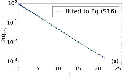
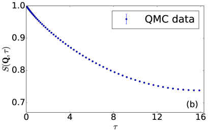
Figure S1: Dynamical spin correlation functions for double-cubic systems with (a) $L=24$ in the QD phase at $g=4.87$ and (b) $L=16$ in the AFM phase at $g=4.724$. A quadratic grid of imaginary times, $\tau_{i}=\Delta i^{2}$, $i=0,1,2,\ldots$, was used in both cases and the inverse temperature was $\beta=2L$. In panel (a), an almost pure exponential decay is observed and the gap is readily extracted from Eq. (S16) of Sec. SIII, giving $\Delta_{T}=0.3028(1)$ (with the error bar estimated by bootstrapping). The spectral functions obtained by analytic continuation are shown in the corresponding panels of Fig. S3.

To carry out the analytic continuation, we use a variant Shao2016 of the SAC approach Sandvik (1998); Beach2004 ; Syljuasen2008 ; Fuchs2010 ; Sandvik2015 , where a chosen parameterization of the spectrum, typically using a large number of $\delta$-functions, is sampled in a Monte Carlo simulation using a likelihood function

$$P(B)\propto\exp(-\chi^{2}[B]/2\Theta),$$ (S13)

where $\Theta$ is a fictitious temperature and thus $\chi^{2}$ plays the role of an energy if the system is regarded as a problem in statistical mechanics. It has been demonstrated Beach2004 that when this formulation is treated in a mean-field-type approximation, it reduces to the more commonly used Maximum Entropy (ME) method Jarrell and Gubernatis (1996). In general, one expects SAC to resolve finer details of the spectrum than ME, because it takes into account fluctuations around the mean-field solution, at the price of requiring long sampling times in certain cases (Refs. Fuchs2010 and Bergeron2016 contain some discussion of this point). The most recent variant of the method Shao2016 , which we deploy here, reduces these sampling times considerably. Typically it delivers simple, single-peak spectral functions in a few minutes or less, when running on a single core, and more complicated spectra, such as the cases with two well-separated peaks that we consider here, in under an hour.

The sampling space is a large number, $N_{\omega}$, of movable $\delta$-functions placed on a frequency grid with a spacing, $\Delta_{\omega}$, sufficiently fine as to be regarded in practice as a continuum (e.g. $\Delta_{\omega}=10^{-5}$). $N_{\omega}$ may range from a value of order $100$ for spectra with little structure to $10^{4}$ or more for complicated spectra. The optimal value also depends on the quality (statistical errors) of the QMC data, with better data requiring larger $N_{\omega}$ for efficient sampling.

At a given instant, the frequency of the $i$th $\delta$-function is $\omega_{i}$, which is an integer multiple of $\Delta_{\omega}$. A sweep consisting of $N_{\omega}$ moves of the type $\omega_{r}\to\omega^{\prime}_{r}$ is performed, with $r$ chosen randomly and the size of the change generated randomly within a window such that approximately half of the updates are accepted. The spectrum is accumulated in a histogram whose bin size is typically much larger than $\Delta_{\omega}$, and is chosen such that all features of the spectrum can be clearly resolved.

In the simplest case, the amplitudes of the $\delta$-functions are all the same, $b_{i}=1/N_{\omega}$, with their value corresponding to a spectrum $B(\omega)$ normalized to unity, as discussed above. We stress that these amplitudes do not have to be changed, and a peak in the spectrum corresponds only to a high average density of $\delta$-functions within a corresponding region. We also carry out simultaneous updates of more than one $\delta$-function, a technique we will discuss in detail elsewhere Shao2016 . The constant amplitudes are intended to reduce the amount of entropic bias Sandvik2015 in the spectrum, and tests indicate that this development does indeed improve the fidelity of the method.

A further refinement is not to use the same amplitude for all $\delta$-functions, but to generate a range of varying amplitudes, such as $b_{i}\propto i$ (with a prefactor chosen to satisfy the standard normalization), and this is the method we employ throughout the current analysis. These amplitudes are kept constant during the sampling process and, because there are no constraints on the locations of the $\delta$-functions, small amplitudes can migrate to areas with lower spectral weight. As long as $N_{\omega}$ is sufficiently large, we find no differences in the final averaged spectrum between the methods of uniform or varying amplitudes. However, the sampling efficiency is increased in the method of varying amplitudes, especially if we include simultaneous amplitude updates of two $\delta$-functions, of the type $b^{\prime}_{i}=b_{j}$, $b^{\prime}_{j}=b_{i}$, with $i$ and $j$ chosen randomly among all the $\delta$-functions. When sampling spectra with two or more peaks, this update leads to considerable improvements in the efficiency of transferring weight between peaks.

An important issue in SAC is how to select the sampling temperature, $\Theta$. The general situation is that a very low $\Theta$ freezes the spectrum close to a stable or metastable $\chi^{2}$ minimum, while a high $\Theta$ leads to large $\chi^{2}$ values, i.e. poor fits to the QMC data for $G(\tau)$. There is a range of $\Theta$ over which the average $\chi^{2}$ value is small but the fluctuations are significant, and cause a smoothing of the spectrum. There is no agreement on exactly how $\Theta$ should be chosen, but in general the different schemes proposed in the literature produce very similar results. This issue is similar to the various ways in which the entropic weighting of the spectrum can be chosen in the ME method Jarrell and Gubernatis (1996); Bergeron2016 .

Here we adopt a simple temperature-adjustment scheme devised in Ref. Shao2016 , where a simulated annealing procedure is first carried out to find the minimum value, $\chi^{2}_{\rm min}$ (in practice this is actually a value close to the minimum, as it may be very difficult to reach the exact global minimum of $\chi^{2}$). After this initial step, $\Theta$ is adjusted so that the average $\chi^{2}$ during the final sampling process for collecting the spectrum satisfies the criterion

$$\langle\chi^{2}\rangle\approx\chi^{2}_{\min}+\sqrt{2N_{\tau}},$$ (S14)

where $N_{\tau}$ is the number of time points in the QMC dataset for $G(\tau)$. With $N_{\tau}$ replaced by $N_{\rm dof}$ (the number of degrees of freedom in a simple fitting procedure), the square-root term would be exactly the standard deviation of the $\chi^{2}$ distribution. With the spectrum constrained to positive frequencies, the number of degrees of freedom is not simply the difference $N_{\tau}-N_{\omega}$, because the sampling parameters, which here are the $N_{\omega}$ frequencies, cannot be considered as independent variables (we note that normally $N_{\omega}\gg N_{\tau}$, whence $N_{\rm dof}$ from the naive definition would be negative and therefore meaningless). We therefore use instead the quantity $\sqrt{2N_{\tau}}$, which typically will be one to two standard deviations of the distribution. This level of noise then corresponds roughly to the removal of distortions due to “fitting to the statistical errors.” In practice, we find that the criterion (S14) produces excellent spectra in tests both on synthetic imaginary-time data and on actual QMC results for systems with known spectral functions Shao2016 .

To illustrate this point, here we show two examples of the results obtained by applying SAC to synthetic QMC data. Our aim is to demonstrate the ability of the advanced SAC method to reproduce a very small secondary peak in the spectrum of precisely the type presented by the amplitude-mode contribution in Figs. 3(a) and 4(a) of the main text. We construct spectra consisting of two Gaussians, with a dominant narrow one at low frequency, containing 98% of the spectral weight, and a weak secondary one at higher frequencies. We consider two different cases. In Fig. S2(a), the secondary peak is also relatively narrow and is separated from the dominant peak by a real gap (a region of zero spectral weight), while in Fig. S2(b) the second peak is broad and there is no gap between the two peaks, but only a region of suppressed spectral weight.

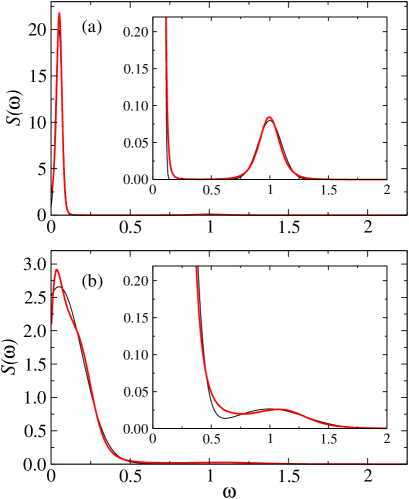
Figure S2: Tests of the advanced SAC method performed using synthetic QMC data. Black curves show artificial spectral functions consisting of two Gaussian peaks. Red curves show the results obtained by applying SAC to the corresponding Green function, $G(\tau)$, with statistical noise generated as described in the text.

To mimic the QMC data underlying the spectra shown in Figs. 3(a) and 4(a) of the main text, we set the inverse temperature to $\beta=50$, use a similar number of $\tau$ points ($N_{\tau}\approx 30$), and generate a noise term, $\sigma_{i}$, to add to the imaginary-time correlation function, $G(\tau_{i})$, corresponding to the artificial spectrum. Given that the QMC data for different $\tau$ points are strongly correlated, we construct correlated noise by averaging independently generated, normally-distributed noise data, $\sigma^{0}_{i}$, using an exponentially decaying weight function,

$$\sigma_{i}=\sum_{j}\sigma^{0}_{i}{\rm e}^{-|i-j|/\xi_{\tau}},$$ (S15)

which we add to $G(\tau_{i})$. We generate a large number of such noisy data sets and run these through the same bootstrapping code that we use for the real QMC data shown in the main text. The correlation time, $\xi_{\tau}$, and the variance of $\sigma^{0}_{i}$ (which is the same for all $i$), are adjusted so that the eigenvalues of the covariance matrix are similar to those of our typical QMC data.

Figure S2(a) shows that the present SAC procedure is fully capable of resolving the secondary peak in the spectrum when there is a gap, with minimal broadening and the correct peak shape. When there is no gap [Fig. S2(b)], the overall shape of the spectrum, including the second peak, is also well reproduced; although the finite spectral weight between the two peaks in this case is larger than in the original spectrum [inset, Fig. S2(b)], decreasing the noise level in the data improves this fit. It is clear from Fig. S2 that advanced SAC methods of the type we apply here are well able to resolve the types of spectral functions expected on physical grounds in all parameter regimes of the system discussed in the main text.

With this demonstration in hand, we conclude this section by showing the spectral functions obtained by applying our SAC method to the imaginary-time data in Fig. S1. In Fig. S3(a), where the system is in the QD phase, only a single narrow triplon peak is found, corresponding to the essentially pure exponential decay seen in Fig. S1(a). By contrast, when the system is in the AFM phase, we observe the two peaks shown in Fig. S3(b), namely the Goldstone mode at $\omega\propto 1/N$ and a smaller peak at higher frequency that corresponds to the amplitude mode, whose scaling properties are discussed in the main text.

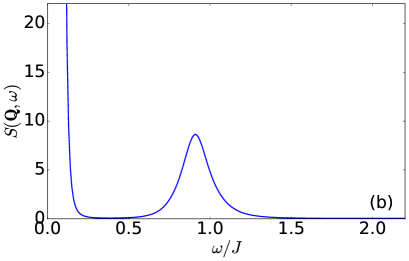
Figure S3: Spectral functions obtained using the SAC method with the imaginary-time data shown in the corresponding panels of Fig. S1. There is no significant spectral weight beyond the frequency ranges shown.

II SIII. Dominant-mode fitting

If a spectral function, $A(\omega)$, contains a single $\delta$-function, the corresponding imaginary-time correlation function, $G(\tau)$, decays exponentially at $T=0$, with the decay constant being the inverse of the gap, $\Delta$. At a finite inverse temperature, $\beta$, the symmetry $G(\beta-\tau)=G(\tau)$ of a bosonic function implies the form

$$G(\tau)=a\cosh[(\beta/2-\tau)\Delta],$$ (S16)

where $a$ is a constant.

Even beyond the single-mode case, this form can in principle always be used to extract the gap of a finite system, whose spectrum is a sum of $\delta$-functions, by fitting to the long-time part of $G(\tau)$, where the lowest-energy $\delta$-function dominates the decay. If the spectral weight of the lowest $\delta$-function, which by definition is exactly at the gap, $\Delta$, is sufficiently large and the second gap to the following $\delta$-function is also sufficiently large, then the asymptotic form of $G(\tau)$ is also given by Eq. (S16) if $\beta$ is sufficiently large. The gap may then be extracted by fitting the large-$\tau$ data. In practice, these conditions can be hard to fulfil rigorously and it becomes necessary to go beyond the single-mode form by performing a fit to more than one exponential, or to perform a still more sophisticated analysis of the long-time decay of the correlation functions. Some methods for this task have been discussed recently Sen2015 ; Suwa2016 .

Figure S1 shows two examples of spin correlation functions from the double-cubic Heisenberg model. In Fig. S1(a), the system is well inside the QD phase and the spectrum at ${\bf q}={\bf Q}=(\pi,\pi,\pi)$ is completely dominated by a single triplon mode. In this case it is easy to extract the gap by fitting to Eq. (S16) and the results are identical to those obtained by SAC [Fig. S3(a)]. By contrast, in Fig. S1(b) the system lies in the AFM phase, close to the QCP, where the resulting spectral function contains both the Goldstone mode, appearing at an energy proportional to $1/N$ and with significant finite-size broadening, and the weak amplitude-mode contribution at higher energies. In this case it is very difficult to extract any information by single-mode fitting and a different technique is required to obtain $A(\omega)$; Fig. S3(b) shows the results obtained by using SAC for this purpose.