Pairing in neutron matter: New uncertainty estimates and three-body forces

Abstract

We present solutions of the BCS gap equation in the channels $\prescript{1\!}{}{S}_{0}$ and $\prescript{3\!}{}{P}_{2}\!-\!\prescript{3\!}{}{F}_{2}$ in neutron matter based on nuclear interactions derived within chiral effective field theory (EFT). Our studies are based on a representative set of nonlocal nucleon-nucleon (NN) plus three-nucleon (3N) interactions up to next-to-next-to-next-to-leading order (N³LO) as well as local and semilocal chiral NN interactions up to N²LO and N⁴LO, respectively. In particular, we investigate for the first time the impact of subleading 3N forces at N³LO on pairing gaps and also derive uncertainty estimates by taking into account results for pairing gaps at different orders in the chiral expansion. Finally, we discuss different methods for obtaining self-consistent solutions of the gap equation. Besides the widely-used quasi-linear method by Khodel et al. we demonstrate that the modified Broyden method is well applicable and exhibits a robust convergence behavior. In contrast to Khodel’s method it is based on a direct iteration of the gap equation without imposing an auxiliary potential and is straightforward to implement.

I Introduction

A quantitative understanding of nuclear superfluidity is central for a wide range of phenomena in nuclear systems, from the structure of nuclei Brink and Broglia (2005); Dean and Hjorth-Jensen (2003) to the cooling of neutron stars Yakovlev and Pethick (2004); Page et al. (2004, 2011). In the inner crust of neutron stars, neutron-rich nuclei form a crystal lattice surrounded by a background liquid of neutrons in a superfluid state (see, e.g., Ref. Gezerlis et al. (2014a) for a review on superfluidity in neutron stars). At densities up to $0.5n_{0}$, with saturation density $n_{0}=0.16\,\mathrm{fm}^{-3}$, neutrons form Cooper pairs in the $\prescript{1\!}{}{S}_{0}$ channel since this channel provides the largest attractive interaction at low momenta. Deeper inside the neutron star, in the outer core, the density increases and at Fermi momenta of $k_{\rm F}\sim 1.5\,\mathrm{fm}^{-1}$ the $\prescript{1\!}{}{S}_{0}$ interaction becomes repulsive and the pairing gap closes in this channel. At these densities the dominant attraction is in the spin-triplet $P$-wave with total angular momentum $J=2$, which is coupled to the $\prescript{3\!}{}{F}_{2}$ channel. Beyond this density it is not obvious to what extent present NN interactions are well constrained by scattering data. Such uncertainties of the interaction are reflected in results for the paring gaps.

Chiral EFT provides a systematic expansion for nuclear forces Epelbaum et al. (2009); Machleidt and Entem (2011), connecting the symmetries of quantum chromodynamics to the interactions between nucleons. Recently, there have been efforts to derive also local chiral interactions Gezerlis et al. (2013, 2014b) as well as semilocal interactions using local regulators for long-range pion exchanges while regulating the short-range contact interactions nonlocally in momentum space Epelbaum et al. (2015a, b). These efforts resulted in sets of NN interactions at different orders in the chiral expansion for a given regulator, which enable more systematic estimates of theoretical uncertainties due to the input nuclear forces.

Neutron pairing gaps in uniform matter have been investigated in the BCS approximation based on chiral interactions, e.g., in Refs. Baldo et al. (1998); Hebeler et al. (2007); Hebeler and Schwenk (2010); Dong et al. (2013); Maurizio et al. (2014); Ding et al. (2016); Srinivas and Ramanan . The BCS approximation is particularly useful to test the sensitivity to nuclear forces. However, we emphasize that there are important contributions beyond the BCS approximation due to screening and vertex corrections, which lead to significant changes to the BCS gaps (for a discussion and further references see Ref. Gezerlis et al. (2014a)). These are not the focus of the present work and are not included in the uncertainties studied here.

In the present paper, we study the zero-temperature pairing gap in neutron matter in the $\prescript{1\!}{}{S}_{0}$ and $\prescript{3\!}{}{P}_{2}\!-\!\prescript{3\!}{}{F}_{2}$ channel based on new local and semilocal NN interactions derived within chiral EFT up to N²LO and N⁴LO, respectively. We also employ an improved method for estimating uncertainties due to the truncation in nuclear forces Epelbaum et al. (2015a, b), which is not based on parameter variation but on an order-by-order analysis in the chiral expansion. For the solution of the gap equation, we show that the modified version of Broyden’s method for solving general nonlinear equations developed in Ref. Johnson (1988) is a powerful method. In combination with the usual method of Khodel et al. Khodel et al. (2001) it allows to assess systematically the iterative convergence. Furthermore, we study the impact of 3N forces on the pairing gap at the level of normal-ordered two-body contributions. Taking advantage of recent developments Hebeler et al. (2015); Drischler et al. (2016) we consider for the first time N³LO 3N contributions to the pairing interaction.

This paper is organized as follows. In Sec. II we discuss details of our calculation, in particular the two independent methods for solving the nonlinear gap equation and the treatment of 3N forces. In Sec. III we present our results for the pairing gap in neutron matter in the $\prescript{1\!}{}{S}_{0}$ and $\prescript{3\!}{}{P}_{2}\!-\!\prescript{3\!}{}{F}_{2}$ channel. We show results for the pairing gap using a free and a Hartree-Fock (HF) single-particle spectrum and also for the effective neutron mass as a function of density for all interactions used. Finally, we summarize and give an outlook in Sec. IV.

II Calculational details

II.1 BCS gap equation

The pairing gap is a $2\times 2$ matrix in single-particle spin space obeying the BCS gap equation at zero-temperature (Baldo et al., 1995)

$$\Delta_{\alpha\alpha^{\prime}}(\mathbf{k})=-\sum\limits_{\begin{subarray}{c}\beta,\beta^{\prime}\\ \mathbf{k}^{\prime}\end{subarray}}\frac{\braket{\mathbf{k}\alpha\alpha^{\prime}}{V}{\mathbf{k}^{\prime}\beta\beta^{\prime}}\Delta_{\beta\beta^{\prime}}(\mathbf{k}^{\prime})}{2\sqrt{\xi^{2}(k^{\prime})+\frac{1}{2}\text{Tr}\left[\Delta\Delta^{\dagger}\right](\mathbf{k}^{\prime})}}\,.$$ (1)

The greek indices indicate the single-particle spin states $\ket{\pm}$, Tr the trace in spin space and $\xi(k)=\varepsilon(k)-\mu$ labels the single-particle energy, e.g., for a free spectrum $\varepsilon(k)=k^{2}/(2m)$ with the neutron mass $m$, relative to the chemical potential $\mu$. Practically, Eq. (1) is solved in a partial-wave representation. We review the decomposition in Appendix A in order to clarify the conventions and approximations used. As shown in the appendix the angular integration can be carried out analytically if the pairing gap in the energy denominator in Eq. (1) is averaged over all spacial directions:

$$\begin{split}\Delta^{2}(k)\equiv\frac{1}{2}\text{Tr}\left[\Delta\Delta^{\dagger}\right]\xrightarrow{\text{av.}}&\frac{1}{2}\int\frac{d\Omega_{\mathbf{k}}}{4\pi}\text{Tr}\left[\Delta\Delta^{\dagger}\right]\\ &=\sum\limits_{l,S,J}|\Delta_{lS}^{J}(k)|^{2}\,.\end{split}$$ (2)

In this approximation the partial-wave decomposed gap equation takes the form Khodel et al. (2001)

$$\Delta_{lS}^{J}(k)=-\int_{0}^{\infty}\frac{dk^{\prime}\,k^{\prime 2}}{\pi}\sum\limits_{l^{\prime}}\frac{i^{l^{\prime}-l}V_{ll^{\prime}S}^{J}(k,k^{\prime})\Delta_{l^{\prime}S}^{J}(k^{\prime})}{\sqrt{\xi^{2}(k^{\prime})+\sum\limits_{\tilde{l},\tilde{S},\tilde{J}}|\Delta_{\tilde{l}\tilde{S}}^{\tilde{J}}(k^{\prime})|^{2}}}\,.$$ (3)

The different angular momenta $l,l^{\prime}=|J\pm 1|$ are coupled in the spin-triplet channel, whereas in the singlet channel we obtain $l^{\prime}=l$. We note that due to the energy denominator the solutions of $\Delta_{lS}^{J}$ are generally coupled, even if the interaction does not couple these channels. However, in practice Eq. (3) can be solved to a very good approximation independently for fixed quantum numbers $S$ and $J$, because they are dominated by the channel in which the pairing interaction is most attractive at a given density. This and angle-averaged gaps are commonly-used approximations (note that the angle-averaging approximation is exact for the $\prescript{1\!}{}{S}_{0}$ channel).

In this paper, we solve Eq. (3) in pure neutron matter for the most attractive channels of the nuclear interactions, the spin-singlet channel $\prescript{1\!}{}{S}_{0}$ and the triplet channel $\prescript{3\!}{}{P}_{2}\!-\!\prescript{3\!}{}{F}_{2}$. The other channels in the triplet $P$-wave, $\prescript{3\!}{}{P}_{0}$ and $\prescript{3\!}{}{P}_{1}$ as well as in higher partial waves are less attractive or even repulsive at the densities considered in this work. We have checked that this also holds with the inclusion of 3N forces. Following Eq. (2) we plot the total gap $\Delta(k_{\rm F})=\sqrt{\sum_{l}\Delta_{l}^{2}(k_{\rm F})}$ evaluated on the Fermi surface to estimate the pairing energy.

II.2 Solving the gap equation

The nonlinear gap equation (3) can be solved iteratively until a self-consistent solution is obtained. However, such approaches are computationally challenging and require more advanced algorithms. The simplest and straightforward method that takes directly the right-hand side of Eq. (3) $I[\ldots]$ in the m-th iteration step,

$${\mathbf{\Delta}_{\text{out}}^{(m)}} =I\left[{\mathbf{\Delta}_{\text{in}}^{(m)}}\right]\quad\text{with}$$ (4a)

$${\mathbf{\Delta}_{\text{in}}^{(m+1)}} ={\mathbf{\Delta}_{\text{out}}^{(m)}}\,,$$ (4b)

converges poorly, if at all. Instead, it typically converges to the (mathematically also valid) trivial solution $\Delta=0$, especially if the nontrivial solution is small. We refer also to Ref. Baran et al. (2008) for a general discussion of iterative methods in the context of nuclear physics. In Eqs. (4) we define a gap vector $\mathbf{\Delta}$ having as components the partial-wave $\Delta_{l}$ sampled each on a Gauss momentum mesh with $N_{p}$ points. The basis size of this vector is $N_{p}$ (spin singlet) and $2\,N_{p}$ (spin triplet), respectively.

In addition to methodical convergence issues, also the evaluation of the integral in Eq. (3) requires some care. Since the pairing gap is typically a small energy scale, the integrand exhibits a strong peak structure for momenta close to the Fermi surface. This quasi-singularity of the BCS gap equation has to be treated carefully when evaluating the integral numerically. We observe that Gauss quadrature converges only if multiple dense integration meshes concentrated around the peak position are well distributed over the entire interval (see also Ref. Baldo et al. (1998)). The presence of the peak makes the integral nevertheless quite sensitive to variations in $\Delta(k_{\rm F})$ and can complicate obtaining a stable self-consistent solution. In order to address these convergence issues, various methods have been applied in the literature, for example the quasi-linear and linear methods of Khodel et al. Khodel et al. (2001) and Krotscheck Krotscheck (1972), or the instability analysis based on in-medium Weinberg eigenvalues Ramanan et al. (2007); Srinivas and Ramanan .

In order to assess the methodical convergence of our results we employ two independent algorithms. These are discussed in detail in the next sections. As it is often referred to, we quantify briefly the term convergence. Let’s consider a general solver that returns the vectors $\mathbf{\Delta}_{\text{in}}^{(m)}$ and $\mathbf{\Delta}_{\text{out}}^{(m)}$ after the $m$-th iteration, specified by an update rule, for instance of the simple form Eq. (4b). The solver is stable if the norm of the difference,

$${\mathbf{F}^{(m)}}={\mathbf{\Delta}_{\text{out}}^{(m)}}-{\mathbf{\Delta}_{\text{in}}^{(m)}}\,,$$ (5)

decreases with $m$, eventually becomes smaller than an arbitrary fixed threshold value and finally a self-consistent solution is found if $|{\mathbf{F}^{(m)}}|=0$. In practice, a small but finite threshold serves as a break condition for the self-consistency cycle. We check the break condition for 5 to 10 additional iterations once it is fulfilled.

II.2.1 Khodel’s method

The method of Khodel et al. has been first presented in Refs. Khodel et al. (1996, 2001) and has since then been widely used in nuclear physics (see, e.g., Refs. Maurizio et al. (2014); Srinivas and Ramanan for recent applications). It is based on a reformulation of the gap equation (3) such that the peak of the integrand, causing the large sensitivity to $\Delta(k_{\rm F})$, is removed. This is achieved by rewriting the potential $V_{ll^{\prime}}(k,k^{\prime})$ in a separable part

$$\phi_{ll^{\prime}}(k)=\frac{V_{ll^{\prime}}(k,k_{\rm F})}{v_{ll^{\prime}}}\quad\text{and}\quad\phi^{T}_{ll^{\prime}}(k^{\prime})=\frac{V_{ll^{\prime}}(k_{\rm F},k^{\prime})}{v_{ll^{\prime}}}\,,$$ (6)

where the definition $v_{ll^{\prime}}=V_{ll^{\prime}}(k_{\rm F},k_{\rm F})\neq 0$ normalizes $\phi_{ll^{\prime}}(k_{\rm F})=\phi^{T}_{ll^{\prime}}(k_{\rm F})=1$, and a remainder

$$W_{ll^{\prime}}(k,k^{\prime})=V_{ll^{\prime}}(k,k^{\prime})-v_{ll^{\prime}}\phi_{ll^{\prime}}(k)\phi_{ll^{\prime}}^{T}(k^{\prime})\,,$$ (7)

which vanishes when at least one argument is on the Fermi surface. This property is key to removing the peak. Inserting the remainder (7) in the gap equation (3) gives

$$\Delta_{l}(k) +\sum\limits_{l^{\prime}}i^{l^{\prime}-l}\int\frac{dk^{\prime}k^{\prime 2}}{\pi}W_{ll^{\prime}}(k,k^{\prime})\frac{\Delta_{l^{\prime}}(k^{\prime})}{\sqrt{\xi^{2}(k^{\prime})+\Delta^{2}(k^{\prime})}}$$

$$=\sum\limits_{l^{\prime}}D_{ll^{\prime}}\phi_{ll^{\prime}}(k)\,,$$ (8)

with the coefficients defined as

$$D_{ll^{\prime}}=-i^{l^{\prime}-l}v_{ll^{\prime}}\int\frac{dkk^{2}}{\pi}\frac{\phi^{T}_{ll^{\prime}}(k)\Delta_{l^{\prime}}(k)}{\sqrt{\xi^{2}(k)+\Delta^{2}(k)}}\,.$$ (9)

The partial-wave gap $\Delta_{l}$ in Eq. (II.2.1) can be written as linear combinations of shape functions $\chi_{l}^{l_{1}l_{2}}(k)$

$$\Delta_{l}(k)=\sum\limits_{l_{1},l_{2}}D_{l_{1}l_{2}}\chi_{l}^{l_{1}l_{2}}(k)\,,$$ (10)

and thus one obtains an equation for the momentum dependence of the partial-wave gaps

$$\chi_{l}^{l_{1}l_{2}}(k) +\sum_{l^{\prime}}i^{l^{\prime}-l}\int\frac{dk^{\prime}k^{\prime 2}}{\pi}W_{ll^{\prime}}(k,k^{\prime})\frac{\chi^{l_{1}l_{2}}_{l^{\prime}}(k^{\prime})}{\sqrt{\xi^{2}(k^{\prime})+\Delta^{2}(k^{\prime})}}$$

$$=\delta_{ll_{1}}\phi_{l_{1}l_{2}}(k)\,.$$ (11)

Since $W_{ll^{\prime}}$ vanishes by construction if at least one argument is on the Fermi surface, the integral in Eq. (II.2.1) is dominated by a momentum region where $\Delta(k)$ is far less important than $\xi(k)$. The shape functions therefore only depend weakly on $\Delta(k)$. This allows to treat Eq. (II.2.1) to a good approximation as quasi-linear, that means by approximating $\Delta(k)$ by a constant. Consequently, the momentum dependence of the gap converges rapidly in Khodel’s method and almost independently of their magnitudes (9) due to the separation (10).

In practice, the iteration scheme works as follows Khodel et al. (2001): each momentum dependence is sampled on a suitable Gauss mesh to ensure convergence of the quadrature. Given $\Delta(k)$ from the previous iteration, one solves Eq. (II.2.1) for the shape functions $\chi_{l}^{l_{1}l_{2}}(k)$ by matrix inversion. For the first iteration a small constant value, e.g., $\Delta(k)=1$ keV, serves as a suitable starting point. We checked that our final results are independent of that choice. The coefficients $D_{ll^{\prime}}$ can then be determined via Eq. (9) combined with Eq. (10) using a nonlinear solver such as the Newton-Raphson method. With the new $D_{ll^{\prime}}$ and $\chi_{l}^{l_{1}l_{2}}(k)$ Eq. (10) updates the partial-wave gaps $\Delta_{l}(k)$. It follows directly from Eq. (II.2.1) that $\chi^{l_{1}l_{2}}_{l}(k_{\rm F})=\delta_{ll_{1}}$ for all $l_{2}$, so the total gap on the Fermi surface for the next iteration step is simply $\Delta_{l}(k_{\rm F})=\sum_{l_{2}}D_{ll_{2}}$. The procedure is repeated until self-consistency is reached, typically within a few iterations.

II.2.2 Modified direct-iteration method

As an alternative to Khodel’s method, we solve for the gap by a modified version of the direct-iteration method in Eqs. (4). Since Eq. (4b) is known to be too simplistic, more advanced update rules are crucial to achieve convergence. As a first step, the stability of the convergence can be significantly improved by dampening the update prescription. The simplest modification involves a linear superposition of the input and output vector of the current iteration:

$${\mathbf{\Delta}_{\text{in}}^{(m+1)}} =\alpha{\mathbf{\Delta}_{\text{out}}^{(m)}}+(1-\alpha){\mathbf{\Delta}_{\text{in}}^{(m)}}$$

$$={\mathbf{\Delta}_{\text{in}}^{(m)}}+\alpha{\mathbf{F}^{(m)}}\,,$$ (12)

where $\alpha$ is the damping factor. We attempted to find suitable values for $\alpha$ that lead to reliable convergence patterns for various NN interactions over a typical range of densities. However, we found that using simple mixing still results in too many discontinuities of the gap as a function of density in order to be useful in practice. These numerical artifacts had to be removed by fine-tuning the damping factor for different densities. Hence, reliable calculations for the gap require more sophisticated updates.

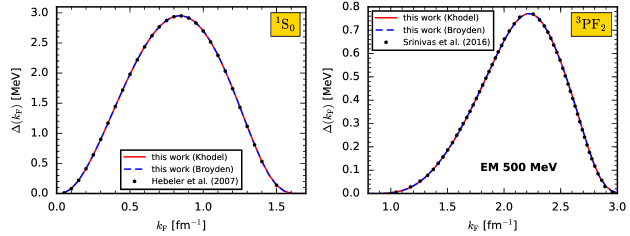
Figure 1: (Color online) Comparison of the gap $\Delta$ as a function of Fermi momentum $k_{\rm F}$ in the $\prescript{1\!}{}{S}_{0}$ (left) and $\prescript{3\!}{}{P}_{2}\!-\!\prescript{3\!}{}{F}_{2}$ (right panel) channel obtained using Khodel’s method (red-solid) and via the new modified direct-iteration method (blue-dashed line). Results are obtained with the N³LO NN potential EM 500 MeV Entem and Machleidt (2003); Machleidt and Entem (2011). Values from Refs. Hebeler et al. (2007); Srinivas and Ramanan are depicted as black dots. The results are in very good agreement, especially, the two methods of this work demonstrate excellent methodical convergence.

We now demonstrate that Broyden’s method for solving general nonlinear equations is in particular well suited for the gap equation (3). Specifically, we make use of a modified version of Broyden’s method developed in Ref. Johnson (1988). It is a fast, stable and computationally efficient quasi-Newton-Raphson method with the advantage of a simple but powerful update rule. The inverse of the Jacobian is approximated by the knowledge of previous iterations without needing to store or to process high-rank matrices. We review here briefly the ingredients to obtain stable results for the gap and refer to the original Ref. Johnson (1988) as well as to Ref. Baran et al. (2008) for first applications to the nuclear many-body problem.

In the modified version of Broyden’s method, the gap vector after the $m$-th iteration is updated according to the rule

$${\mathbf{\Delta}_{\text{in}}^{(m+1)}}={\mathbf{\Delta}_{\text{in}}^{(m)}}+\alpha{\mathbf{F}^{(m)}}-\sum\limits_{n=1}^{m-1}w_{n}\gamma_{mn}{\mathbf{u}^{(n)}}\,,$$ (13)

with the definitions

$$\gamma_{mn} =\sum\limits_{k=1}^{m-1}c_{km}\beta_{kn}\,,$$ (14)

$$\beta_{kn} =(w_{0}^{2}\mathds{1}+a)_{kn}^{-1}\,,$$ (15)

$$c_{km} =w_{k}\,{\delta\mathbf{F}^{(k)\dagger}\mathbf{F}^{(m)}}\,,$$ (16)

$$a_{kn} =w_{k}w_{n}\,{\delta\mathbf{F}^{(n)\dagger}\delta\mathbf{F}^{(k)}}\,,$$ (17)

and

$${\mathbf{u}^{(n)}} =\alpha\,{\delta\mathbf{F}^{(n)}}+{\delta\mathbf{\Delta}^{(n)}}\,,$$ (18)

$${\delta\mathbf{\Delta}^{(n)}} =\frac{{\mathbf{\Delta}_{\text{in}}^{(n+1)}}-{\mathbf{\Delta}_{\text{in}}^{(n)}}}{\left|{\mathbf{F}^{(n+1)}}-{\mathbf{F}^{(n)}}\right|}\,,$$ (19)

$${\delta\mathbf{F}^{(n)}} =\frac{{\mathbf{F}^{(n+1)}}-{\mathbf{F}^{(n)}}}{\left|{\mathbf{F}^{(n+1)}}-{\mathbf{F}^{(n)}}\right|}\,,$$ (20)

where $\delta\mathbf{F}^{(n)}$ is normalized, ${\delta\mathbf{F}^{(n)\dagger}\delta\mathbf{F}^{(n)}}=1$. The procedure requires to store ${\mathbf{\Delta}_{\text{in}}^{(m)}}$ and $\mathbf{F}^{(m)}$ of the current iteration as well as ${\mathbf{u}^{(m)}}$ and ${\delta\mathbf{F}^{(m)}}$ of all previous steps. Since $a_{kn}$ is typically of rank much smaller than that of the full Jacobian it can be stored for efficiency. Although the update rule (13) includes simple mixing, the additional correction allows usually larger damping factors $\alpha$, which typically leads to accelerated convergence. Besides guesses for $\mathbf{\Delta}_{\text{in}}^{(1)}$ and $\alpha$, the weights $w_{m}$ have to be chosen as well, whereas $w_{0}=0.01$ needs to be sufficiently small Johnson (1988). We use $w_{m}=1$, $m\geqslant 1$, similar to Ref. Baran et al. (2008). In addition, Ref. Johnson (1988) suggested $w_{m}=\min\left(1,\sqrt{(\mathbf{F}^{(m)\dagger}\mathbf{F}^{(m)})^{-1}}\right)$ to promote solutions of advanced convergence.

We show in Fig. 1 an exemplary benchmark for the gap $\Delta(k_{\rm F})$ obtained with Khodel’s (red-solid) and with the modified direct-iteration method (blue-dashed lines) in comparison to the literature (points) Hebeler et al. (2007); Srinivas and Ramanan . The gaps are based on the N³LO NN potential EM 500 MeV Entem and Machleidt (2003); Machleidt and Entem (2011) in the channels $\prescript{1\!}{}{S}_{0}$ (left) and $\prescript{3\!}{}{P}_{2}\!-\!\prescript{3\!}{}{F}_{2}$ (right panel). We observe in general almost perfect agreement (deviations are of order of $10$ eV) of the two methods for the singlet as well as the triplet channel. We used the same optimized Gauss mesh for the two methods. Furthermore, the results in Fig. 1 agree well with the literature, also in the regions of small gaps. In practice, Khodel’s method requires typically $2$ to $3$ times fewer steps to converge while the computational runtime is shorter for the modified direct-iteration method due to its simplicity. In rare cases the modified direct-iteration method leads to apparent discontinuities in the gap as a function of $k_{\rm F}$. In all of our calculations we could easily recover these by modifying slightly the damping factor $\alpha$. On the other hand, Khodel’s method in its usual implementation is naturally unstable if the $V_{ll^{\prime}}(k,k)$ gets small or has in particular nodes.

Based on these benchmarks, we conclude that the two algorithms are equally reliable. Comparing the results of Khodel’s method and the modified direct-iteration method allows us to assess the methodical convergence of our calculations. The results of the following sections could therefore be obtained with either of the methods.

II.3 Three-nucleon forces, normal ordering and single-particle energies

Our calculations are based on NN and 3N interactions up to N³LO in the chiral expansion. The contributions from 3N forces are taken into account at the normal-ordered two-body level. Normal-ordering with respect to a given reference state allows to include the dominant 3N contributions in terms of density-dependent two-body interactions $\overline{V}_{\text{3N}}^{\text{as}}$ Holt et al. (2010); Hebeler and Schwenk (2010); Carbone et al. (2014); Drischler et al. (2016); Wellenhofer et al. (2016). Specifically, normal ordering of 3N forces in neutron matter involves the summation of one particle over occupied states in the Fermi sea:

$$\overline{V}_{\text{3N}}^{\text{as}}=\text{Tr}_{\sigma_{3}}\int\frac{d\mathbf{k}_{3}}{(2\pi)^{3}}\mathcal{A}_{123}V_{\text{3N}}\,n_{\mathbf{k}_{3}}\bigg{|}_{\text{nnn}}\,,$$ (21)

where the Fermi-Dirac distribution function is given at zero temperature by a simple step function, $n_{\mathbf{k}}=\theta\left(k_{\rm F}-|\mathbf{k}|\right)$, and the Fermi momentum $k_{\rm F}$ associated with the particle density by $n=k_{\rm F}^{3}/(3\pi^{2})$. The antisymmetrized 3N interactions $\mathcal{A}_{123}V_{\text{3N}}$ used in this work are regularized by the nonlocal regulator $f_{\text{R}}(p,q)=\exp[-((p^{2}+3q^{2}/4)/\Lambda_{\text{3N}}^{2})^{4}]$, where $p,q$ are the Jacobi momenta and $\Lambda_{\text{3N}}$ is the 3N cutoff scale.

The contributions of 3N forces at N²LO to the BCS pairing gap have already been studied via normal ordering, see, e.g., Refs. Hebeler and Schwenk (2010); Dong et al. (2013); Maurizio et al. (2014); Srinivas and Ramanan . The calculation of $\overline{V}_{\text{3N}}^{\text{as}}$ can be performed directly based on the operator structure of the 3N interactions as in Refs. Hebeler and Schwenk (2010); Holt et al. (2010). However, this approach becomes rather cumbersome for subleading 3N forces at N³LO due to the complex operator structure of 3N interactions at this order. In order to study N³LO 3N contributions we make use of recent developments Hebeler et al. (2015); Drischler et al. (2016) and evaluate the effective NN potentials (21) using the partial-wave decomposition of the 3N forces. The partial-wave matrix elements of the 3N forces, $\Braket{p^{\prime}q^{\prime}\alpha^{\prime}}{\mathcal{A}_{123}V_{\text{3N}}}{pq\alpha}$, are given in a $Jj$-coupled 3N plane-wave basis of the form

$$\Ket{pq\alpha}=\Ket{pq;\left[(LS)J\left(l\frac{1}{2}\right)j\right]\mathcal{J}\left(T\frac{1}{2}\right)\mathcal{T}}\,,$$ (22)

where the relative orbital angular momentum, spin, total angular momentum, and isospin of particles $1$ and $2$ are labeled by $L$, $S$, $J$, and $T$ (with $T=1$ in the case of neutron matter). The quantum numbers $l$ and $j$, respectively, denote the orbital angular momentum and total angular momentum of particle $3$ relative to the center of mass of the pair with relative momentum $p$. The quantum numbers $\mathcal{J}$ and $\mathcal{T}$ are the total 3N angular momentum and isospin (with $\mathcal{T}=3/2$ here). These 3N matrix elements are currently available up to N³LO Hebeler et al. (2015), with a large enough truncation on the total three- and two-body total angular momenta $\mathcal{J}\leqslant 9/2$ and $J\leqslant 6$, respectively, to obtain well converged 3N Hartree-Fock energies in neutron and symmetric nuclear matter Hebeler et al. (2015); Drischler et al. (2016). We refer to these references also for detailed discussions of normal ordering in the partial-wave basis. The effective NN potential (21) depends in general on the total momentum $\mathbf{P}$ of the two remaining particles in contrast to a Galilean-invariant NN interaction. At the BCS level, the paired particles are in back-to-back kinematics and we therefore have $\mathbf{P}=0$.

The normal-ordered two-body part of 3N forces can then be combined with NN interactions:

$$V_{\text{NN+3N}}^{\text{as}}=V_{\text{NN}}^{\text{as}}+\zeta\,\overline{V}_{\text{3N}}^{\text{as}}\,,$$ (23)

where $\zeta$ is a combinatorial factor that depends on the type of quantity of interest (see Ref. Hebeler and Schwenk (2010) for details). For the gap equation (3) we find $\zeta=1$ (see Appendix B for details).

The energy denominator of the gap equation (3) depends on the single-particle energy $\varepsilon(k)$. We take into account self-energy corrections to the kinetic energy due to the interaction (23). In the Hartree-Fock approximation the single-particle energy is given by

$$\varepsilon(k)=\frac{k^{2}}{2m}+\Sigma^{(1)}(k)\,,$$ (24)

where $\Sigma^{(1)}(k)$ denotes the spin-averaged Hartree-Fock self-energy Hebeler and Schwenk (2010),

$$\begin{split}\Sigma^{(1)}(k_{1})&=\frac{1}{2\pi}\int dk_{2}\,k_{2}^{2}\int d\cos\theta_{\mathbf{k}_{1},\mathbf{k}_{2}}\,n_{\mathbf{k}_{2}}\sum_{l,S,J}(2J+1)\\ &\quad\times\Braket{k_{12}/2}{V_{llS}^{J}}{k_{12}/2}\left(1-(-1)^{l+S+1}\right)\,,\end{split}$$ (25)

with $k_{12}=|\mathbf{k}_{1}-\mathbf{k}_{2}|$. For the combinatorial factor $\zeta$ in the interaction matrix element $V=V_{\text{NN+3N}}^{\text{as}}$ in Eq. (25) we obtain $\zeta=1/2$ (see Appendix B or Refs. Hebeler and Schwenk (2010); Srinivas and Ramanan ; Drischler et al. (2016)). The corresponding effective mass $m^{*}$ at the Fermi surface is then given by

$$\frac{m^{*}(k_{\rm F})}{m}=\left(\frac{m}{k}\frac{d\varepsilon(k)}{dk}\right)^{-1}\bigg{|}_{k=k_{\rm F}}\,.$$ (26)

Our calculations with a free and a Hartree-Fock spectrum serve as a simple measure for the dependence of $\Delta(k_{\rm F})$ on the single-particle energy.

II.4 Theoretical uncertainties

An improved approach for estimating theoretical uncertainties based on the chiral expansion has been proposed in Refs. Epelbaum et al. (2015a, b) and applied to few-body calculations Binder et al. (2016); Lynn et al. (2016). In contrast to previous uncertainty estimates, which involved cutoff variations of nuclear interactions at a given chiral order, these are based on results at different chiral orders for a fixed cutoff value. This allows to study the order-by-order convergence in the chiral expansion for an observable at a given momentum scale. Currently, local Gezerlis et al. (2013, 2014b) and semilocal Epelbaum et al. (2015a, b) NN potentials are available up to N²LO and N⁴LO, respectively, with cutoffs of $R_{0}=(0.8-1.2)\,\mathrm{fm}$. Semilocal means in this context that only the long-range part is regularized locally in coordinate space whereas the short-range part is regularized nonlocally in momentum space.

The contributions to the gap from interaction terms at chiral order $i=0,2,3,\ldots$ are given by

$$\mathrm{d}\Delta^{(i)}=\begin{cases}\Delta^{(2)}-\Delta^{(0)}&i=2\,,\\ \Delta^{(i)}-\Delta^{(i-1)}&i\geqslant 3\,,\end{cases}$$ (27)

and are expected to scale like $\bigl{(}Q(k_{\rm F})\bigr{)}^{i}$ where

$$Q(k_{\rm F})=\max\left(\frac{p}{\Lambda_{b}},\frac{m_{\pi}}{\Lambda_{b}}\right)\,$$ (28)

is the ratio of a typical momentum scale $p$ or $m_{\pi}$ of the system and the breakdown scale $\Lambda_{b}$. Since the pairing gap results from attractive interactions of two particles on the Fermi surface we use in the following $p=k_{\rm F}$ for the relative momentum in Eq. (28). Note that this scaling is in general only expected to be valid for complete calculations involving all many-body forces at a given chiral order. In Sec. III we present results based on local and semilocal interactions without inclusion of many-body forces. Complete calculations with full uncertainty estimates will be possible as soon as partial-wave matrix elements of the corresponding 3N forces are available. For the local and semilocal NN interactions the breakdown scale was chosen as follows for the different cutoffs $R_{0}$ Epelbaum et al. (2015a):

$$\Lambda_{b}=\begin{cases}600\,\mathrm{MeV}&\text{for}\;R_{0}=0.8,0.9,1.0\,\mathrm{fm}\,,\\ 500\,\mathrm{MeV}&\text{for}\;R_{0}=1.1\,\mathrm{fm}\,,\;\text{and}\\ 400\,\mathrm{MeV}&\text{for}\;R_{0}=1.2\,\mathrm{fm}\,.\end{cases}$$ (29)

The chiral expansion can be used to define the theoretical uncertainty Epelbaum et al. (2015b, a), where we focus on uncertainties at N²LO and higher ($i\geqslant 3$),

$$\delta\Delta^{(i)}=\max\limits_{3\leqslant j\leqslant i}\left(Q^{i+1-j}\left|\mathrm{d}\Delta^{(j)}\right|\right)\,.$$ (30)

We do not show uncertainties at LO and NLO, because at these orders the scattering phase shifts are not well reproduced at the relevant momenta, particularly not in the coupled $\prescript{3\!}{}{P}_{2}\!-\!\prescript{3\!}{}{F}_{2}$ channel. Note that, in contrast to Refs. Epelbaum et al. (2015b, a), for the above reason we neglect the LO contributions to the higher-order uncertainties, and moreover we do not consider a term that ensures that the next order always lies within the uncertainty band of the previous order by taking into account information of higher-order results in the chiral expansion.

As mentioned in Sec. II.3, the normal ordering is currently based on 3N forces with nonlocal regulators. Once available, it will be straightforward to incorporate also local or semilocal 3N interactions. Work in this direction is currently in progress. Following the paradigm to regularize NN and many-body forces consistently, we do not show results based on local or semilocal NN forces combined with nonlocal 3N interactions. Instead, we use the nonlocal N³LO NN potentials EM 500 MeV Entem and Machleidt (2003); Machleidt and Entem (2011), EGM 450/500 MeV and EGM 450/700 MeV Epelbaum et al. (2005) with the 3N uncertainty estimate governed by variation of the 3N parameters $c_{1},c_{3}$ and $\Lambda_{\text{3N}}=(2.0-2.5)\,\mathrm{fm}^{-1}$. As recommended in Ref. Krebs et al. (2012), we take for calculations with N²LO 3N forces the ranges $c_{1}=-(0.37-0.73)\,\mathrm{GeV}^{-1}$, $c_{3}=-(2.71-3.38)\,\mathrm{GeV}^{-1}$ and with N³LO 3N forces $c_{1}=-(0.75-1.13)\,\mathrm{GeV}^{-1}$, $c_{3}=-(4.77-5.51)\,\mathrm{GeV}^{-1}$. The N³LO 3N contributions shift $c_{1},c_{3}$ and depend additionally on the LO NN low-energy constants which we consider consistently with the NN potentials. A compilation of the values can be found in Table I of Ref. Krüger et al. (2013).

III Results

III.1 Local and semilocal NN potentials

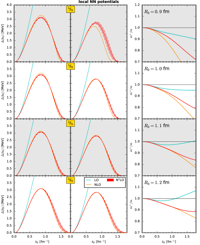
Figure 2: (Color online) Gap $\Delta$ as a function of Fermi momentum $k_{\rm F}$ in the $\prescript{1\!}{}{S}_{0}$ channel for the four local NN potentials with $R_{0}=(0.9-1.2)\,\mathrm{fm}$ (rows) each up to N²LO with a free (left) and a Hartree-Fock spectrum (center column), respectively. The third column shows the effective mass at the Fermi surface corresponding to the Hartree-Fock spectrum (second column). As discussed in the text, the uncertainty bands (if present) are given by the color-filled region between the dashed lines while the actual calculation is depicted by the solid line. There are no uncertainties shown for LO and NLO; for details see text.

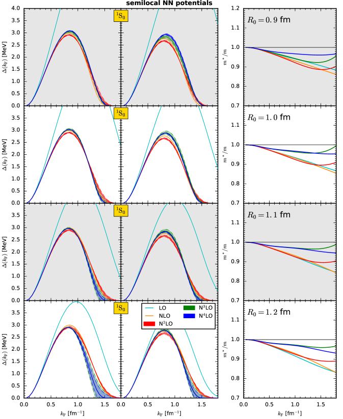
Figure 3: (Color online) Gap $\Delta$ as a function of Fermi momentum $k_{\rm F}$ in the $\prescript{1\!}{}{S}_{0}$ channel for the four semilocal NN potentials with $R_{0}=(0.9-1.2)\,\mathrm{fm}$ (rows) each up to N⁴LO with a free (left) and a Hartree-Fock spectrum (center column), respectively. The third column shows the effective mass at the Fermi surface corresponding to the Hartree-Fock spectrum (second column). There are no uncertainties shown for LO and NLO; for details see text.

We present in Figs. 2 and 3 the gap in the ${}^{1}S_{0}$ channel based on the local and semilocal NN potentials up to N²LO and N⁴LO, respectively. Each row corresponds to the regulators $R_{0}=0.9,1.0,1.1$ and $1.2\,\mathrm{fm}$ as annotated. The left (center) column shows the gap using a free (Hartree-Fock) spectrum. The effective mass $m^{*}(k_{\rm F})/m$ from the Hartree-Fock spectrum are depicted in the right column. As discussed in Sec. II.4 we assign uncertainty estimates to the results beyond NLO according to Eq. (30). In Figs. 2 and 3 the results for $\Delta(k_{\rm F})$ at different orders are depicted by solid lines, and the uncertainty bands $\Delta(k_{\rm F})\pm\delta\Delta$ are shown as shaded bands whose boundaries are highlighted by dashed lines. We restrict the bands to the region of positive energies.

At NLO and beyond we observe that the $\prescript{1\!}{}{S}_{0}$ gap agrees up to $k_{\rm F}\sim(0.6-0.8)\,\mathrm{fm}^{-1}$, depending only slightly on the regulator for local potentials. As investigated in detail, e.g., in Ref. Hebeler et al. (2007), the pairing gaps are strongly constrained by phase shifts. The LO gaps are therefore expected to be different. For $R_{0}\geqslant 1.0\,\mathrm{fm}$ we find that the gaps at N³LO and N⁴LO agree well over the entire density range. Generally, the gap uncertainties based on Eq. (30) are very small for the highest chiral orders. However, we emphasize that the gap uncertainties only include contributions from the chiral expansion, whereas neglected higher-order many-body corrections are not assessed.

In addition, we find that the sensitivity of the pairing gap to the energy spectrum is rather small and affects mainly the maximum value of the gap. For both, local and semilocal potentials we find $\Delta_{\text{max}}\sim(2.7-3.1)\,\mathrm{MeV}$ at $k_{\rm F}\sim(0.8-0.9)\,\mathrm{fm}^{-1}$ for the highest chiral order and all cutoffs. The rather small suppression due to the spectrum can be directly understood based on the fact that the ratio $m^{*}(k_{\rm F})/m$ is close to one for all regulators and chiral orders (right columns).

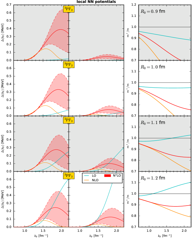
Figure 4: (Color online) Gap $\Delta$ as a function of Fermi momentum $k_{\rm F}$ in the $\prescript{3\!}{}{P}_{2}\!-\!\prescript{3\!}{}{F}_{2}$ channel for the four local NN potentials with $R_{0}=(0.9-1.2)\,\mathrm{fm}$ (rows), each up to N²LO with a free (left) and a Hartree-Fock spectrum (center column), respectively. The third row shows the effective mass at the Fermi surface corresponding to the Hartree-Fock spectrum (second column). As discussed in the text, the uncertainty bands (if present) are given by the color-filled region between the dashed lines while the actual calculation is depicted by the solid line. There are no uncertainties shown for LO and NLO; for details see text.

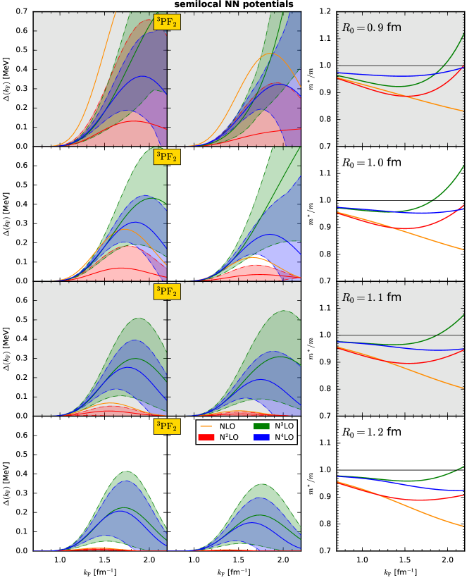
Figure 5: (Color online) Gap $\Delta$ as a function of Fermi momentum $k_{\rm F}$ in the $\prescript{3\!}{}{P}_{2}\!-\!\prescript{3\!}{}{F}_{2}$ channel for the four semilocal NN potentials with $R_{0}=(0.9-1.2)\,\mathrm{fm}$ (rows), each up to N⁴LO with a free (left) and a Hartree-Fock spectrum (center column), respectively. The third row shows the effective mass at the Fermi surface corresponding to the Hartree-Fock spectrum (second column). As discussed in the text, the uncertainty bands are given by the color-filled region between the dashed lines while the actual calculation is depicted by the solid line. There are no uncertainties shown for LO and NLO; for details see text.

In Figs. 4 and 5 we show the $\prescript{3\!}{}{P}_{2}\!-\!\prescript{3\!}{}{F}_{2}$ gap based on the same NN potentials. Since $\prescript{3\!}{}{P}_{2}\!-\!\prescript{3\!}{}{F}_{2}$ pairing takes place at larger densities than in the $\prescript{1\!}{}{S}_{0}$ channel, the uncertainties are much larger. The maximum of the LO pairing gap for the local potentials changes significantly with increasing $R_{0}$, indicating that the results are strongly affected by regulator artifacts at this order. On the other hand, the pairing gap for the semilocal potentials at LO is vanishing for all densities and cutoff values and therefore not shown in Fig. 5. These results reflect the poor description of the phase shifts at this order, from only the one-pion-exchange interaction at this order for the semilocal case.

At higher chiral orders it is not straightforward to extract robust quantitative trends for the $\prescript{3\!}{}{P}_{2}\!-\!\prescript{3\!}{}{F}_{2}$ gap. In general, the gap opens around densities of $k_{\rm F}\sim 1\,\mathrm{fm}^{-1}$ for all considered interactions. For the semilocal potentials the results at N³LO and N⁴LO agree well up to $k_{\rm F}\sim 1.6\,\mathrm{fm}^{-1}$. Also the corresponding uncertainty bands strongly overlap in this density region. We find the maximum gap values at N²LO and higher orders in the density range $k_{\rm F}=(1.6-2.1)\,\mathrm{fm}^{-1}$ for all interactions. Overall, the large uncertainties at high densities reflect the regulator dependences and the breakdown of the chiral expansion. In particular, for a Fermi momentum $k_{\rm F}=2.0\,\mathrm{fm}^{-1}$ the expansion parameter $Q(k_{\rm F})$ of Eq. (28) is

$$Q(2.0\,\mathrm{fm}^{-1})=\begin{cases}0.66&\text{for}\;R_{0}=0.8,0.9,1.0\,\mathrm{fm}\,,\\ 0.79&\text{for}\;R_{0}=1.1\,\mathrm{fm}\,,\;\text{and}\\ 0.99&\text{for}\;R_{0}=1.2\,\mathrm{fm}\,.\end{cases}$$ (31)

Clearly, it is not obvious that the chiral expansion is efficient anymore in this density regime.

III.2 N²LO and N³LO 3N forces

We also study the pairing gaps based on three nonlocal NN potentials at N³LO combined with contributions from N²LO and N³LO 3N forces. The results are shown in Figs. 6 and 7 in the $\prescript{1\!}{}{S}_{0}$ and $\prescript{3\!}{}{P}_{2}\!-\!\prescript{3\!}{}{F}_{2}$ channel, respectively. The rows correspond to the NN potential EM 500 MeV Entem and Machleidt (2003), EGM 450/500 MeV and EGM 450/700 MeV Epelbaum et al. (2005), as annotated. The left and center columns show energy gaps using a free and Hartree-Fock spectrum, whereas the right column shows the corresponding Hartree-Fock effective mass. NN-only results are shown by black solid lines, with the inclusion of the leading (subleading) 3N forces by orange (blue) bands. As discussed in Sec. II.4, the uncertainty bands are obtained by variations of the 3N parameters $c_{1},c_{3}$ and $\Lambda_{\text{3N}}$.

Figs. 2, 3 and 6 show that the $\prescript{1\!}{}{S}_{0}$ gaps at N³LO without 3N forces are in good agreement. This observation can be traced back to the well-reproduced phase shifts at this order. Contributions from 3N forces do not change the results for the pairing gaps at low densities, $k_{\rm F}\lesssim(0.7-0.8)\,\mathrm{fm}^{-1}$, and only lead to a minor suppression at higher densities. The uncertainty bands including 3N forces are very small for all potentials at N²LO as well as N³LO. In addition, self-energy contributions to the single-particle energies are small.

In Fig. 7 we show the corresponding results for the $\prescript{3\!}{}{P}_{2}\!-\!\prescript{3\!}{}{F}_{2}$ channel. Since the relevant densities are larger than in the $\prescript{1\!}{}{S}_{0}$ channel, the impact of 3N forces is generally larger for the pairing gap and also for the effective mass. We observe nonvanishing gaps for the three investigated NN potentials for all three cases considered. In contrast to the $\prescript{1\!}{}{S}_{0}$ channel the inclusion of 3N forces typically provides additional attraction and hence increases the pairing gap, except for the EM 500 MeV potential with subleading 3N forces. As shown in the right column, 3N contributions generally tend to enhance the effective mass (see also Ref. Hebeler and Schwenk (2010)), even to values larger than one at the Hartree-Fock level. In general, we find that the results for the $\prescript{3\!}{}{P}_{2}\!-\!\prescript{3\!}{}{F}_{2}$ pairing gaps differ significantly for the various potentials and that it is delicate to extract robust quantitative predictions based on our results.

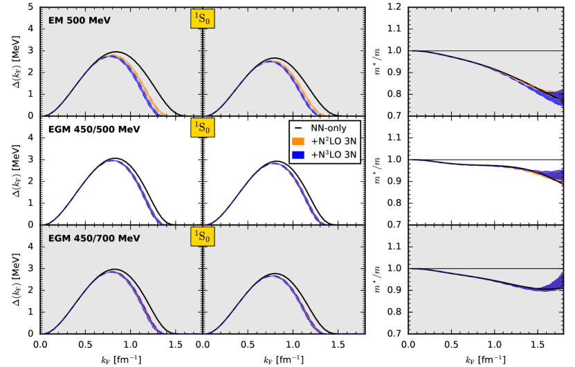
Figure 6: (Color online) Gap $\Delta$ as a function of Fermi momentum $k_{\rm F}$ in the $\prescript{1\!}{}{S}_{0}$ channel with a free (left) and a Hartree-Fock spectrum (center column) for the N³LO NN potentials EM 500 MeV (first), EGM 450/500 MeV (second) and EGM 450/700 MeV (third row). The third column depicts the effective mass at the Fermi surface corresponding to the Hartree-Fock spectrum. The NN-only results are shown by the black-solid lines. The uncertainty bands for N²LO and N³LO are determined by variations of the 3N parameters $c_{1},c_{3}$ and $\Lambda_{\text{3N}}$ as discussed in the text.

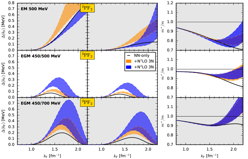
Figure 7: (Color online) Gap $\Delta$ as a function of Fermi momentum $k_{\rm F}$ in the $\prescript{3\!}{}{P}_{2}\!-\!\prescript{3\!}{}{F}_{2}$ channel with a free (left) and a Hartree-Fock spectrum (center column) for the N³LO NN potentials EM 500 MeV (first), EGM 450/500 MeV (second) and EGM 450/700 MeV (third row). The third column depicts the effective mass at the Fermi surface corresponding to the Hartree-Fock spectrum. The NN-only results are shown by the black-solid lines. The uncertainty bands for N²LO and N³LO are determined by variations of the 3N parameters $c_{1},c_{3}$ and $\Lambda_{\text{3N}}$ as discussed in the text.

IV Summary and Outlook

In this paper, we have studied solutions of the BCS gap equation in the $\prescript{1\!}{}{S}_{0}$ and the $\prescript{3\!}{}{P}_{2}\!-\!\prescript{3\!}{}{F}_{2}$ channel based on a broad range of nuclear interactions derived within chiral EFT at different chiral orders. We benchmarked and optimized two different algorithms that allow a reliable and accurate solution of the nonlinear BCS equation. With these advances, we studied the gap based on local NN interactions Gezerlis et al. (2013, 2014b) up to N²LO and semilocal NN interactions Epelbaum et al. (2015a, b) up to N⁴LO for the four coordinate-space cutoffs $R_{0}=0.9,1.0,1.1$ and $1.2$ fm. At the highest chiral orders the results in the $\prescript{1\!}{}{S}_{0}$ channel agree for all interactions over the entire density region. The $\prescript{1\!}{}{S}_{0}$ pairing gap reaches a maximum around $k_{\rm F}=(0.8-0.9)\,\mathrm{fm}^{-1}$ with $\Delta_{\text{max}}=(2.9-3.3)\,\mathrm{MeV}$ for a free single-particle spectrum and a suppression of about $\sim 0.3\,\mathrm{MeV}$ when including self-energy corrections in the Hartree-Fock approximation.

In the triplet channel $\prescript{3\!}{}{P}_{2}\!-\!\prescript{3\!}{}{F}_{2}$ the situation is much less clear. The gaps generally open at densities of $k_{\rm F}\sim(0.9-1.0)\,\mathrm{fm}^{-1}$ for all interactions. Beyond this density the results depend on details of the interactions and the chiral order. At the highest chiral orders we observe a gap maximum at densities in the region $k_{\rm F}=(1.7-1.9)\,\mathrm{fm}^{-1}$ with $\Delta_{\text{max}}<0.4\,\mathrm{MeV}$. However, we emphasize that these Fermi-momentum scales are already close to the EFT breakdown scale of the corresponding interactions. Consequently, the observed strong regulator dependence is not surprising.

For the estimate of theoretical order-by-order uncertainties of the Hamiltonian we followed the method first presented in Ref. Epelbaum et al. (2015a) with two modifications. We obtained very small uncertainties for the $\prescript{1\!}{}{S}_{0}$ channel for all densities, but sizable uncertainties in the $\prescript{3\!}{}{P}_{2}\!-\!\prescript{3\!}{}{F}_{2}$ channel. In the latter case the uncertainty bands at successive chiral orders are generally not entirely overlapping. However, at N³LO and N⁴LO we find that the bands are of comparable size and overlapping. We emphasize that our calculations at N²LO, N³LO and N⁴LO are not complete since no 3N forces have been taken into account for these interactions. Hence, the analysis should be revisited as soon as the calculation of the corresponding local 3N partial-wave matrix elements have been completed. This is work in progress.

In addition, we also investigated the impact of 3N forces on the pairing gap for nonlocal N³LO potentials. Taking advantage of recent developments for including 3N forces in a partial-wave basis Hebeler et al. (2015); Drischler et al. (2016), we were able to incorporate for the first time subleading 3N contributions in the gap equation via normal ordering. We found only small repulsive effects from 3N forces in the singlet channel $\prescript{1\!}{}{S}_{0}$, whereas in the $\prescript{3\!}{}{P}_{2}\!-\!\prescript{3\!}{}{F}_{2}$ channel the effects from 3N forces are larger and lead to attractive contributions in most cases. Also for these interactions, we find significant regulator dependences in the $\prescript{3\!}{}{P}_{2}\!-\!\prescript{3\!}{}{F}_{2}$ channel.

We conclude that due to the high densities of the $\prescript{3\!}{}{P}_{2}\!-\!\prescript{3\!}{}{F}_{2}$ gaps, which are reaching the limit of the employed chiral EFT interactions, it is not possible to draw final quantitative conclusions on the size of the $\prescript{3\!}{}{P}_{2}\!-\!\prescript{3\!}{}{F}_{2}$ gap in neutron matter. However, we have observed nonvanishing gaps for all employed realistic NN potentials, also when including 3N contributions. We further emphasize that the contributions from higher many-body corrections beyond the BCS approximation have not been taken into account and are known to be significant Gezerlis et al. (2014a); Schwenk and Friman (2004), although their quantitative assessment is especially challenging in the $\prescript{3\!}{}{P}_{2}\!-\!\prescript{3\!}{}{F}_{2}$ channel.

The methods discussed in this paper can be used for improved studies of pairing gaps in the future. In particular, the advanced treatment of 3N forces in terms of partial waves allows to handle in a straightforward way arbitrary partial-wave decomposed 3N forces. In addition, it is also possible to perform calculations based on consistently-evolved NN and 3N forces Hebeler (2012) via the similarity renormalization group (SRG). This is in particular of interest when taking into account many-body corrections beyond the BCS approximation in calculations of the pairing gap since SRG-evolved forces are expected to exhibit an improved many-body convergence.

Appendix A Partial-wave decomposition

In this appendix we briefly review the partial-wave decomposition of the gap equation (3) and specify the conventions used in this work. Following Refs. (Clark et al., 2003; Takatsuka, 1970; Khodel et al., 2001) we decompose the gap matrix in the form

$$\Delta_{\alpha\alpha^{\prime}}(\mathbf{k})=\sum\limits_{\begin{subarray}{c}l,S\\ J,M\end{subarray}}\sqrt{\frac{8\pi}{2J+1}}\,\Delta_{lS}^{JM}(k)\left(G_{lS}^{JM}(\hat{\mathbf{k}})\right)_{\alpha\alpha^{\prime}}\,,$$ (32)

and accordingly the nuclear interaction

$$\begin{split}&(4\pi)^{-2}\braket{\mathbf{k}\alpha\alpha^{\prime}}{V}{\mathbf{k}^{\prime}\beta\beta^{\prime}}\\ &=\sum\limits_{\begin{subarray}{c}l,l^{\prime},S\\ J,M\end{subarray}}i^{l^{\prime}-l}\left(G_{lS}^{JM}(\hat{\mathbf{k}})\right)_{\alpha\alpha^{\prime}}\left(G_{l^{\prime}S}^{JM}(\hat{\mathbf{k}}^{\prime})\right)_{\beta\beta^{\prime}}^{*}V_{ll^{\prime}S}^{J(M)}(k,k^{\prime})\,,\end{split}$$ (33)

with

$$\left(G_{lS}^{JM}(\hat{\mathbf{k}})\right)_{\alpha\alpha^{\prime}}=\sum\limits_{m,m_{S}}\mathcal{C}_{1/2\alpha 1/2\alpha^{\prime}}^{Sm_{S}}\mathcal{C}_{lmSm_{S}}^{JM}Y_{l}^{m}(\hat{\mathbf{k}})\,.$$ (34)

These functions obey the orthogonality relations

$$\begin{split}\int d\Omega_{\mathbf{k}}&\sum_{\beta,\beta^{\prime}}\left[\left(G_{l^{\prime}S}^{JM}(\hat{\mathbf{k}}^{\prime})\right)_{\beta\beta^{\prime}}^{*}\left(G_{l^{\prime\prime}S^{\prime}}^{J^{\prime}M^{\prime}}(\hat{\mathbf{k}}^{\prime})\right)_{\beta\beta^{\prime}}\right]\\ &=\delta_{ll^{\prime}}\delta_{MM^{\prime}}\delta_{JJ^{\prime}}\delta_{SS^{\prime}}\,.\end{split}$$ (35)

The $J$-dependent factor in Eq. (32) is chosen such that the gap equation in partial-wave representation takes a particularly simple form. Inserting Eqs. (32) and (33) in the gap equation (1) leads to

$$\begin{split}&(4\pi)^{-2}\sum\limits_{\begin{subarray}{c}l,S\\ J,M\end{subarray}}\frac{\Delta_{lS}^{JM}(k)}{\sqrt{2J+1}}\left(G_{lS}^{JM}(\hat{\mathbf{k}})\right)_{\alpha\alpha^{\prime}}\\ &=-\int\frac{dk^{\prime}\,k^{\prime 2}}{(2\pi)^{3}}\sum\limits_{\begin{subarray}{c}l,l^{\prime},J,M,S\\ l^{\prime\prime},J^{\prime},M^{\prime},S^{\prime}\end{subarray}}i^{l^{\prime}-l}\left(G_{lS}^{JM}(\hat{\mathbf{k}})\right)_{\alpha\alpha^{\prime}}\\ &\quad\times V_{ll^{\prime}S}^{J(M)}(k,k^{\prime})\frac{\Delta_{l^{\prime\prime}S^{\prime}}^{J^{\prime}M^{\prime}}(k^{\prime})}{\sqrt{2J^{\prime}+1}}\\ &\quad\times\int d\Omega_{\mathbf{k}^{\prime}}\frac{\sum_{\beta,\beta^{\prime}}\left[\left(G_{l^{\prime}S}^{JM}(\hat{\mathbf{k}}^{\prime})\right)_{\beta\beta^{\prime}}^{*}\left(G_{l^{\prime\prime}S^{\prime}}^{J^{\prime}M^{\prime}}(\hat{\mathbf{k}}^{\prime})\right)_{\beta\beta^{\prime}}\right]}{2\sqrt{\xi^{2}(k^{\prime})+\frac{1}{2}\text{Tr}\left[\Delta\Delta^{\dagger}\right](\mathbf{k}^{\prime})}}\,.\end{split}$$ (36)

This equation can be simplified significantly by averaging the energy gap in the denominator over all angles, specifically

$$\begin{split}\frac{1}{2}\text{Tr}\left[\Delta\Delta^{\dagger}\right]&\xrightarrow{\text{av.}}\frac{1}{2}\int\frac{d\Omega_{\mathbf{k}}}{4\pi}\text{Tr}\left[\Delta\Delta^{\dagger}\right]\\ &=\sum\limits_{l,S,J}|\Delta_{lS}^{J}(k^{\prime})|^{2}\equiv D^{2}(k)\,.\end{split}$$ (37)

Here we summed over all $M$ states and used identity (35). Projecting out the components in Eq. (36) leads to the partial-wave decomposed gap equation

$$\Delta_{lS}^{J}(k)=-\int_{0}^{\infty}\frac{dk^{\prime}\,k^{\prime 2}}{\pi}\sum\limits_{l^{\prime}}\frac{i^{l^{\prime}-l}V_{ll^{\prime}S}^{J}(k,k^{\prime})\Delta_{l^{\prime}S}^{J}(k^{\prime})}{\sqrt{\xi^{2}(k^{\prime})+\sum\limits_{\tilde{l},\tilde{S},\tilde{J}}|\Delta_{\tilde{l}\tilde{S}}^{\tilde{J}}(k^{\prime})|^{2}}}\,.$$ (38)

Appendix B Normal-ordering symmetry factors

In this section we discuss the symmetry factor $\zeta$ that appears in the interaction kernel in Eq. (23) for normal-ordered 3N contributions in the normal self-energy $\Sigma$ and the anomalous self-energy $\Delta$. For this we consider a general Hamiltonian of the form

$$\hat{H}=\hat{T}+\hat{V}_{\text{NN}}+\hat{V}_{\text{3N}}\,,$$ (39)

where $\hat{T}$ represents the kinetic energy, $\hat{V}_{\text{NN}}$ all two-nucleon interactions and $\hat{V}_{\text{3N}}$ three-nucleon interactions. By using Wick’s theorem we can recast the Hamiltonian exactly in an equivalent form by normal ordering all operators with respect to a given reference state. For the treatment of superfluid systems it is convenient to choose the BCS state as reference state. We represent $\hat{V}_{\text{NN}}$ and $\hat{V}_{\text{3N}}$ in terms of antisymmetrized matrix elements:

$$\hat{V}_{\text{NN}} =\frac{1}{4}\sum_{ijkl}\left<ij|V^{\rm as}_{\text{NN}}|kl\right>\hat{a}_{i}^{\dagger}\hat{a}_{j}^{\dagger}\hat{a}_{l}\hat{a}_{k}\,,$$ (40)

$$\hat{V}_{\text{3N}} =\frac{1}{36}\sum_{ijklmn}\left<ijk|V^{\rm as}_{\text{3N}}|lmn\right>\hat{a}_{i}^{\dagger}\hat{a}_{j}^{\dagger}\hat{a}_{k}^{\dagger}\hat{a}_{n}\hat{a}_{m}\hat{a}_{l}\,,$$ (41)

where the indices represent generic single-particle quantum numbers. When applying Wick’s theorem with respect to a BCS reference state it is important to note that both normal contractions (connecting a creation operator with an annihilation operator) as well as anomalous contractions (connecting two creation or two annihilation operators) contribute. For the normal self-energy $\Sigma$ the relevant contractions are of the form

$$\frac{1}{4}\sum_{ijkl}\left<ij|V^{\rm as}_{\text{NN}}|kl\right>\contraction[1.0ex]{\hat{a}_{i}^{\dagger}}{\hat{a}_{j}^{\dagger}}{}{\hat{a}_{l}}\hat{a}_{i}^{\dagger}\hat{a}_{j}^{\dagger}\hat{a}_{l}\hat{a}_{k}\,,$$ (42)

$$\frac{1}{36}\sum_{ijklmn}\left<ijk|V^{\rm as}_{\text{3N}}|lmn\right>\contraction[1.0ex]{\hat{a}_{i}^{\dagger}\hat{a}_{j}^{\dagger}}{\hat{a}_{k}^{\dagger}}{}{\hat{a}_{n}}\contraction[1.5ex]{\hat{a}_{i}^{\dagger}}{\hat{a}_{j}^{\dagger}}{\hat{a}_{k}^{\dagger}\hat{a}_{n}}{\hat{a}_{m}}\hat{a}_{i}^{\dagger}\hat{a}_{j}^{\dagger}\hat{a}_{k}^{\dagger}\hat{a}_{n}\hat{a}_{m}\hat{a}_{l}\,,$$ (43)

whereas for the anomalous self-energy $\Delta$ the relevant contractions take the form

$$\frac{1}{4}\sum_{ijkl}\left<ij|V^{\rm as}_{\text{NN}}|kl\right>\contraction[1.0ex]{}{\hat{a}_{i}^{\dagger}}{}{\hat{a}_{j}^{\dagger}}\hat{a}_{i}^{\dagger}\hat{a}_{j}^{\dagger}\hat{a}_{l}\hat{a}_{k}\,,$$ (44)

$$\frac{1}{36}\sum_{ijklmn}\left<ijk|V^{\rm as}_{\text{3N}}|lmn\right>\contraction[1.0ex]{\hat{a}_{i}^{\dagger}\hat{a}_{j}^{\dagger}}{\hat{a}_{k}^{\dagger}}{}{\hat{a}_{n}}\contraction[1.0ex]{}{\hat{a}_{i}^{\dagger}}{}{\hat{a}_{j}^{\dagger}}{}\hat{a}_{i}^{\dagger}\hat{a}_{j}^{\dagger}\hat{a}_{k}^{\dagger}\hat{a}_{n}\hat{a}_{m}\hat{a}_{l}\,.$$ (45)

Since the interaction operators are represented in terms of antisymmetrized matrix elements all different possible choices of picking creation or annihilation operators are equivalent and just lead to combinatoric factors. Hence, in order to determine $\zeta$ it is necessary to determine the number of different contractions $c_{N}$ for Eqs. (42) to (45). We obtain: $c_{N}=4$ for (42), $c_{N}=18$ for (43), $c_{N}=1$ for (44) and $c_{N}=9$ for (45). Combining these combinatoric factors with the prefactors $1/4$ and $1/36$ of the NN and 3N interactions we directly obtain $\zeta=1/2$ for $\Sigma$ and $\zeta=1$ for $\Delta$. We also note that in the present work we approximate the normal contractions in (45) by their contributions in normal systems. It has been shown in Ref. Carbone et al. (2014) that the inclusion of correlations in the reference state has only very small effects on the matrix elements of the normal-ordered 3N contributions for nuclear matter calculations. In addition to contributions from normal contractions in (45) we also obtain nonvanishing contributions from multiple anomalous contractions. However, these contributions are small since such terms only include contributions from momenta around the Fermi surface and are of higher order in the gap.

References

- Brink and Broglia (2005) D. M. Brink and R. A. Broglia, Nuclear Superfluidity: Pairing in Finite Systems, Cambridge Monographs on Particle Physics, Nuclear Physics and Cosmology, Vol. 24 (Cambridge University Press, 2005).
- Dean and Hjorth-Jensen (2003) D. J. Dean and M. Hjorth-Jensen, Rev. Mod. Phys. 75, 607 (2003).
- Yakovlev and Pethick (2004) D. G. Yakovlev and C. J. Pethick, Ann. Rev. Astron. Astrophys. 42, 169 (2004).
- Page et al. (2004) D. Page, J. M. Lattimer, M. Prakash, and A. W. Steiner, Astrophys. J. Suppl. Ser. 155, 623 (2004).
- Page et al. (2011) D. Page, M. Prakash, J. M. Lattimer, and A. W. Steiner, Phys. Rev. Lett. 106, 081101 (2011).
- Gezerlis et al. (2014a) A. Gezerlis, C. J. Pethick, and A. Schwenk, in Novel Superfluids: Volume 2, International Series of Monographs on Physics, Vol. 157, edited by K.-H. Bennemann and J. B. Ketterson (Oxford University Press, Oxford, 2014) Chap. 22, p. 580.
- Epelbaum et al. (2009) E. Epelbaum, H.-W. Hammer, and U.-G. Meißner, Rev. Mod. Phys. 81, 1773 (2009).
- Machleidt and Entem (2011) R. Machleidt and D. R. Entem, Phys. Rep. 503, 1 (2011).
- Gezerlis et al. (2013) A. Gezerlis, I. Tews, E. Epelbaum, S. Gandolfi, K. Hebeler, A. Nogga, and A. Schwenk, Phys. Rev. Lett. 111, 032501 (2013).
- Gezerlis et al. (2014b) A. Gezerlis, I. Tews, E. Epelbaum, M. Freunek, S. Gandolfi, K. Hebeler, A. Nogga, and A. Schwenk, Phys. Rev. C 90, 054323 (2014b).
- Epelbaum et al. (2015a) E. Epelbaum, H. Krebs, and U.-G. Meißner, Eur. Phys. J. A 51, 53 (2015a).
- Epelbaum et al. (2015b) E. Epelbaum, H. Krebs, and U.-G. Meißner, Phys. Rev. Lett. 115, 122301 (2015b).
- Baldo et al. (1998) M. Baldo, Ø. Elgarøy, L. Engvik, M. Hjorth-Jensen, and H.-J. Schulze, Phys. Rev. C 58, 1921 (1998).
- Hebeler et al. (2007) K. Hebeler, A. Schwenk, and B. Friman, Phys. Lett. B 648, 176 (2007).
- Hebeler and Schwenk (2010) K. Hebeler and A. Schwenk, Phys. Rev. C 82, 014314 (2010).
- Dong et al. (2013) J. M. Dong, U. Lombardo, and W. Zuo, Phys. Rev. C 87, 062801 (2013).
- Maurizio et al. (2014) S. Maurizio, J. W. Holt, and P. Finelli, Phys. Rev. C 90, 044003 (2014).
- Ding et al. (2016) D. Ding, A. Rios, H. Dussan, W. H. Dickhoff, S. J. Witte, A. Carbone, and A. Polls, Phys. Rev. C 94, 025802 (2016).
- (19) S. Srinivas and S. Ramanan, “Triplet Pairing in pure neutron matter,” arXiv:1606.09053 .
- Johnson (1988) D. D. Johnson, Phys. Rev. B 38, 12807 (1988).
- Khodel et al. (2001) V. V. Khodel, V. A. Khodel, and J. W. Clark, Nucl. Phys. A 679, 827 (2001).
- Hebeler et al. (2015) K. Hebeler, H. Krebs, E. Epelbaum, J. Golak, and R. Skibinski, Phys. Rev. C 91, 044001 (2015).
- Drischler et al. (2016) C. Drischler, K. Hebeler, and A. Schwenk, Phys. Rev. C 93, 054314 (2016).
- Baldo et al. (1995) M. Baldo, U. Lombardo, and P. Schuck, Phys. Rev. C 52, 975 (1995).
- Baran et al. (2008) A. Baran, A. Bulgac, M. M. Forbes, G. Hagen, W. Nazarewicz, N. Schunck, and M. V. Stoitsov, Phys. Rev. C 78, 014318 (2008).
- Krotscheck (1972) E. Krotscheck, Z. Phys. 251, 135 (1972).
- Ramanan et al. (2007) S. Ramanan, S. Bogner, and R. J. Furnstahl, Nucl. Phys. A 797, 81 (2007).
- Khodel et al. (1996) V. A. Khodel, V. V. Khodel, and J. W. Clark, Nucl. Phys. A 598, 390 (1996).
- Entem and Machleidt (2003) D. R. Entem and R. Machleidt, Phys. Rev. C 68, 041001(R) (2003).
- Holt et al. (2010) J. W. Holt, N. Kaiser, and W. Weise, Phys. Rev. C 81, 024002 (2010).
- Carbone et al. (2014) A. Carbone, A. Rios, and A. Polls, Phys. Rev. C 90, 054322 (2014).
- Wellenhofer et al. (2016) C. Wellenhofer, J. W. Holt, and N. Kaiser, Phys. Rev. C 93, 055802 (2016).
- Binder et al. (2016) S. Binder, A. Calci, E. Epelbaum, R. J. Furnstahl, J. Golak, K. Hebeler, H. Kamada, H. Krebs, J. Langhammer, S. Liebig, P. Maris, U. G. Meißner, D. Minossi, A. Nogga, H. Potter, R. Roth, R. Skibinski, K. Topolnicki, J. P. Vary, and H. Witała (LENPIC Collaboration), Phys. Rev. C 93, 044002 (2016).
- Lynn et al. (2016) J. E. Lynn, I. Tews, J. Carlson, S. Gandolfi, A. Gezerlis, K. E. Schmidt, and A. Schwenk, Phys. Rev. Lett. 116, 062501 (2016).
- Epelbaum et al. (2005) E. Epelbaum, W. Glöckle, and U.-G. Meißner, Nucl. Phys. A 747, 362 (2005).
- Krebs et al. (2012) H. Krebs, A. Gasparyan, and E. Epelbaum, Phys. Rev. C 85, 054006 (2012).
- Krüger et al. (2013) T. Krüger, I. Tews, K. Hebeler, and A. Schwenk, Phys. Rev. C 88, 025802 (2013).
- Schwenk and Friman (2004) A. Schwenk and B. Friman, Phys. Rev. Lett. 92, 082501 (2004).
- Hebeler (2012) K. Hebeler, Phys. Rev. C 85, 021002(R) (2012).
- Clark et al. (2003) J. W. Clark, V. A. Khodel, and M. V. Zverev, in Condensed Matter Theories, Vol. 17, edited by M. P. Das and F. Green (Nova Science Publishers, New York, 2003) Chap. 2, p. 23, nucl-th/0203046 .
- Takatsuka (1970) T. Takatsuka, Prog. Theor. Phys. 44, 905 (1970).