STM driven transition from rippled to buckled graphene in a spin-membrane model

Abstract

We consider a simple spin-membrane model for rippling in graphene. The model exhibits transitions from a flat but rippled membrane to a buckled one. At high temperature the transition is second order but it is first order at low temperature for appropriate strength of the spin-spin coupling. Driving the system across the first order phase transition in nonequilibrium conditions that mimic interaction of the graphene membrane with a STM tip explains recent experiments. In particular, we observe a reversible behavior for small values of the STM current and an irreversible transition from flat rippled membrane to rigid buckled membrane when the current surpasses a critical value. This work opens the possibility to test mechanical properties of graphene under different temperature and electrostatic conditions.

I Introduction

Rippling in suspended graphene mey07 is one of its most compelling mechanical properties, and is usually linked to the impossibility of finding a perfect crystal in two dimensions mermin . Thus, the out-of-plane displacements would make it possible to stabilize the graphene sample. The understanding of this rippling has triggered a great amount of theoretical work, both starting from first principles fas07 ; abe07 ; kim08 ; gazit09 ; san-jose ; gui14 ; gonzalez ; ByR16 and using simple statistical mechanics models jsm12bon ; pre12bon ; Ruiz-Garcia ; prb12bon ; schoelz15 .

The typical length of these graphene ripples, which do not have a preferred direction mey07 ; pss09ban , is in the nanometer range. Moreover, they modify the electronic band structure of graphene PRB08gui and are expected to have a prominent role in its electronic transport PTRS08kat . There have been many attempts to characterize ripples as equilibrium phenomena, connecting them with thermal fluctuations fas07 ; abe07 and the electron-phonon coupling kim08 ; gazit09 . Also, some authors have tried to describe their curvature starting from first principles gonzalez ; gui14 .

Recently, there has been a growing interest in buckling of suspended graphene both for theoretical reasons and for its role in designing graphene-based devices. There are many experimental studies of buckled graphene sheets SN88 ; CN93 ; leh13 ; kot14 ; rob14 ; BCGW15 ; lin12 ; svensson11 ; xu14 ; schoelz15 , including some very recent ones in which Molecular Dynamics (MD) simulations are also carried out neek-amal ; ackerman . Buckling can be produced by the application of strong enough electrostatic forces, as in refs. lin12 ; svensson11 , by the combination of heating and an electrostatic force, as in ref. schoelz15 or even by only heating the sample, as in the “mirror” buckling observed in ackerman by means of MD simulations.

Buckling upon heating a graphene sample has been systematically investigated in ref. schoelz15 by using scanning tunneling microscopy (STM). Specifically, the tip of the microscope is centered on a suspended sample that is initially flat on average although it is surely covered with ripples mey07 . Application of a voltage bias $V$ between the STM tip and the membrane has a twofold effect: (i) it induces a tunneling current that locally heats the sample, and (ii) it produces an electrostatic interaction between the tip and the sample. Experiments show that the suspended graphene sheet experiences a transition from “floppy” rippled-flat to “rigid” buckled state. The membrane height $Z$ is plotted in Fig. 1 as a function of the voltage bias $V$ for several values of the tunneling intensity $I$. On the one hand, for “small” values of $I$, the height $Z=Z(V)$ is a monotone increasing and continuous function of $V$. The membrane is rippled and its behavior is reversible: the same curve $Z(V)$ is observed whether the voltage bias increases from $0$ to a certain value $V_{\max}$ or decreases from $V_{\max}$ to $0$. On the other hand, once the current is kept constant at a high enough value, increasing the bias causes the sample to buckle irreversibly: once a sufficiently large value $V_{\max}$ is reached, the sample remains buckled as the bias is decreased back from $V_{\max}$ to zero.

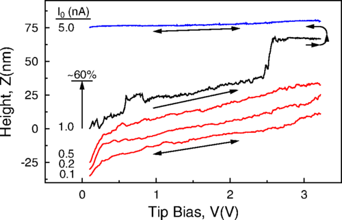
Figure 1: Height of the STM tip on the graphene sheet versus applied voltage for different values of the tunneling current. Curves are slightly offset from each other for clarity. From ref.  schoelz15 .

Schoelz et al proposed a phenomenological Ising model to explain their experimental results schoelz15 . In their model, each local spin $\sigma_{ij}$ represents one ripple composed of $\sim 1000$ carbon atoms and the value of the spin indicates the curvature of the ripple. The energy of this Ising system has two contributions. Firstly, a nearest neighbor spin-spin interaction, with a coupling constant $J$ that depends on the total magnetization $M=\sum_{ij}\sigma_{ij}$. The second contribution to the energy is an interaction of the spins with an external field $h=h_{0}e^{-r/\xi}$, where $h_{0}$ is assimilated to the voltage bias in the experiment and $r$ is the distance to the center of the sample, located just “below” the STM tip. The spin-spin interaction is antiferromagnetic ($J=-1$) for $0<M<M_{0}$ and ferromagnetic ($J=2$) for $M>M_{0}$, $M_{0}$ is $60\%$–$70\%$ of the maximum possible value of the magnetization. The correlation length $\xi$ may also change discontinuously and, counterintuitively, the temperature decreases as the tunneling current increases schoelz15 . The $M$ versus $h$ curve of this model is as follows schoelz15 . At zero field, $M=0$ and thus $J=-1$. As $h_{0}$ increases to $h_{0}^{\text{max}}=3$, the spin-spin interaction reverses suddenly to ferromagnetic ($J=2$) at a field $h_{0}\simeq 2.5$ for which $M$ has reached $M_{0}$. This discontinuous increase in $J$ at $h_{0}=2.5$ causes a sudden increase of the magnetization. Afterwards, when the external field is decreased back to $0$, the coupling constant is left unchanged at $J=2$ and therefore the spins never go back to the initial state. To further mimic experimental results, a smaller jump in the magnetization for $h_{0}<2.5$ is induced by an increase in the correlation length $\xi$; see Figure 3 in ref. schoelz15 .

In this paper, we qualitatively explain Schoelz et al’s experimental findings schoelz15 by using a spin-membrane model that exhibits ripples on a flat membrane, buckling and a dynamical transition from floppy to rigid states. Thus we do not need to: (i) interpret spins as many-atom ripples, (ii) introduce jumps in $J$ and $\xi$ with $M$, and (iii) decrease the temperature with increasing tunneling current, as done in ref. schoelz15 . Our model includes coupling between out-of-plane elastic displacements of atoms and local pseudo-spins that pull atoms off plane. The pseudo-spins are coupled by nearest neighbor interactions. In a previous publication, we have analyzed a similar model under constant, low, temperature conditions Ruiz-Garcia . STM experiments occur under varying temperature conditions because of Joule heating due to the tunneling current. Increasing the temperature is akin to driving the system through a first-order phase transition, which is the essence of our explanation of Schoelz et al’s experiments. Thus in the present work we include: (a) an external field that represents the STM voltage and, most importantly, (b) the (non-homogeneous) time-dependent temperature profile brought about by the STM heating of the sample. For different values of control parameters, first and second order phase transitions between a rippled-flat membrane state and a buckled state appear. In the parameter region where these phases coexist, it is possible to drive the system in conditions that mimic those in the experiment: inhomogeneous sample heating due to the tunneling current and electrostatic tip-sample interaction schoelz15 . We then show that the wrinkled to buckled transition appears naturally in our model, without having to invoke ad-hoc jumps in the model parameters. Moreover, the spin-membrane model reproduces all the key experimental observations in the STM experiment, while providing a reasonable physical picture of the real system.

The plan of the paper is as follows. The spin-membrane model in a hexagonal lattice is introduced in section II. The different equilibrium phases are numerically characterized in section III, in which we show that there is a first order phase transition between a flat but rippled membrane and a buckled one. In section IV, we drive the system through the first order phase transition in conditions similar to those in the experiments. A discussion of our results is presented in section V.

II The model on a hexagonal lattice

Here, we briefly present our 2d model and its governing equations. Similar models include simpler 0d spin-oscillator jstat10 ; jstat10a , 1d spin-string pre12bon and 2d spin-membrane jsm12bon models. More complex models include spin-membrane coupling as well as next neighbor and nearest next neighbor spin-spin couplings Ruiz-Garcia . All these models exhibit phase transitions between a flat membrane state and a buckled state below some critical temperature. Additional transitions occur in the model that has short-ranged spin-spin interactions Ruiz-Garcia . There are different phases characterized by two order parameters: the magnetization and a domain length parameter that gives information about the pseudo-spins spatial correlations. For a hexagonal lattice, there are buckled phases with non-vanishing global magnetization and also rippled phases with zero magnetization Ruiz-Garcia . The pseudo-spins are partially correlated in space in these latter phases, which comprise long wavelength phases, analogous to those in refs. mey07 ; pss09ban , stripy phases as in ASC11mao , and atomic wavelength phases, similar to the ordered phases in ref. nl12oha . Earlier theoretical studies of buckling in membranes include the existence of a critical temperature for buckling in polymerized sheets Guitter88 and buckling in graphene due to doping gazit09 .

Carbon atoms are placed on a hexagonal lattice as shown in Fig. 2. Let $(\sigma_{ij}$, $u_{ij}$, $p_{ij})$ be the values of the atom pseudo-spin, height and momentum, respectively, at site $(i,j)$. The Hamiltonian is

$$\mathcal{H}=\sum_{ij}\left(\frac{p_{ij}^{2}}{2m}-fu_{ij}\sigma_{ij}\right)+\sum_{|i-j|=\text{even}} \Bigg{\{}\frac{k}{2}\big{[}(u_{ij}-u_{i+1,j})^{2}+(u_{ij}-u_{i,j-1})^{2}+(u_{ij}-u_{i,j+1})^{2}\big{]}$$

$$+J\sigma_{ij}(\sigma_{i+1,j}+\sigma_{i,j-1}+\sigma_{i,j+1})\Bigg{\}}.$$ (1)

This is a particular case of the Hamiltonian introduced in ref. Ruiz-Garcia that had an additional next-nearest-neighbor interaction among spins.

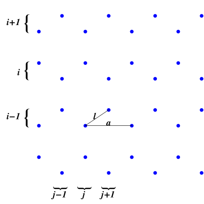
Figure 2: Figure summarizing the atom indices and the parameters of the unit cell of the hexagonal lattice. In doing this plot, we have indexed files and rows assuming that $|i-j|$ is even.

The dynamics of the system consists of (i) Hamilton’s equations of motion for $(u_{ij},p_{ij})$, and (ii) Glauber dynamics Gl63 at temperature $T$ for $\sigma_{ij}$:

$$\ddot{u}_{ij}-K_{N}^{2}(u_{i+1,j}+u_{i,j-1}+u_{i,j+1}-3u_{ij})=\sigma_{ij},$$ (2)

$$\omega_{ij}(\bm{\sigma}|\bm{u})=\frac{\delta}{2}(1-\gamma_{ij}\sigma_{ij}),$$ (3)

$$\gamma_{ij}=\tanh\left[\frac{u_{ij}}{\theta}-\frac{\kappa}{\theta}(\sigma_{i+1,j}+\sigma_{i,j+1}+\sigma_{i,j-1})\right]\!.$$ (4)

Here $\omega_{ij}$ is the rate at which the pseudo-spin at site $(i,j)$ flips and $\delta$ is a parameter setting the characteristic time-scale for the pseudo-spin flips. In the long time limit, the system reaches thermodynamic equilibrium and its probability distribution has the canonical form $\mathcal{P}\propto\exp(-\mathcal{H}/T)$. It is convenient to introduce the following parameters,

$$T_{0}=\frac{f^{2}K_{N}^{2}}{k},\quad K_{N}=\frac{3n-2}{\sqrt{6}\pi},$$ (5)

where $n$ is the total number of rows in the lattice. The temperature $T_{0}$ is the transition temperature from a (high temperature) flat to a buckled string configuration for $J=0$ Ruiz-Garcia . Then, we define dimensionless displacements and time,

$$u_{ij}^{*}=\frac{ku_{ij}}{fK_{N}^{2}},\qquad t^{*}=\frac{t}{K_{N}}\sqrt{\frac{k}{m}},$$ (6)

and also dimensionless spin-spin coupling constant and temperature,

$$\kappa=\frac{J}{T_{0}},\quad\theta=\frac{T}{T_{0}}=\frac{k\,T}{f^{2}K_{N}^{2}}.$$ (7)

Thus we measure energy in units of the transition temperature $T_{0}$.

In the equilibrium state, the average dimensionless displacements obey the discrete Poisson equation

$$-K_{N}^{2}(u_{i+1,j}+u_{i,j-1}+u_{i,j+1}-3u_{ij})=\mu_{ij},$$ (8)

in which $\mu_{ij}$ stands for the average magnetization at site $(i,j)$. The asterisks have been omitted so as not to clutter the formulae. In the continuum limit, Eq. (8) becomes

$$\frac{1}{2\pi^{2}}\nabla^{2}u(x,y)=\mu(x,y).$$ (9)

Here $0\leq x,y\leq 1$, and the sample becomes the unit square in the continuum limit with our choice of dimensionless variables Ruiz-Garcia . Therefore, the average magnetization gives the curvature of the membrane. Thus we can deduce the state of the membrane by looking at either the atoms displacements $u(x,y)$ or the pseudo-spins local value $\mu(x,y)$.

III Equilibrium Phase Diagrams

Except for $J=0$ that can be exactly solved, the equilibrium phase diagrams have to be calculated numerically. At $J=0$, the flat solution bifurcates at $T=T_{0}$ to a buckled state, which is thermodynamically stable for $T<T_{0}$ Ruiz-Garcia . This can be appreciated in Fig. 3, which has been drawn by down-sweeping the dimensionless temperature from a given $\theta>1$ at each fixed value of $\kappa$. At the largest value of $\theta$, the initial configuration is random and the simulation reaches equilibrium after a certain time. Then, the magnetization $M$ and the domain length parameter $\mathcal{DL}$ of ref. nl12oha ,

$$M = \left|\frac{1}{N}\sum_{ij}\sigma_{ij}\right|\!,$$ (10)

$$\mathcal{DL} = \frac{1}{3N}\sum_{|i-j|=\text{even}}\left[3+\sigma_{ij}\left(\sigma_{i+1,j}+\sigma_{i,j-1}+\sigma_{i,j+1}\right)\right].$$ (11)

are registered. For the next simulation, $\theta$ is slightly lowered and the equilibrium configuration reached at the previous temperature is used as the initial condition. This procedure is continued until the phase diagram is completed. The parameter $\mathcal{DL}$ gives information about the difference between the number of ferromagnetic (contributing +1 to $\mathcal{DL}$) and antiferromagnetic (contributing -1 to $\mathcal{DL}$) links and makes it possible to discriminate between different phases with zero global magnetization. Specifically, we have $\mathcal{DL}=1/2$ for random pseudo-spins and $\mathcal{DL}=0$ for antiferromagnetic ordering. For ferromagnetic ordering, it is $M=\mathcal{DL}=1$. Note that the magnetization (10) does not discriminate between the two possible signs of the curvature in Eq. (9).

The method we have just described produces the correct phase diagram provided the phase transitions are second order, which is the case for high critical temperatures ($\theta>0.5$ as seen in Fig. 3). For first order phase transitions, down-sweeping yields only one part of the hysteresis loops associated with first order phase transitions, specifically that corresponding to the stable phase at the higher temperatures. To visualize the thermodynamically stable phase at first order phase transitions that occur for low critical temperatures, $\theta<0.5$, we have redrawn the diagram always starting simulations from a random configuration and waiting for the system to equilibrate. This produces Fig. 4. On the one hand, we observe that there is a region of zero magnetization at low temperatures (approximately, $0.07<\kappa<0.2$) that was absent in Fig. 3. In this region, the membrane is rippled as shown by its partial antiferromagnetic ordering, $0\leq{\cal DL}\leq 0.1$. On the other hand, the membrane ends up in low temperatures states that are similar to those in Fig. 3 both for $\kappa\lesssim 0.07$ (buckled membrane) and $\kappa\gtrsim 0.2$ (rippled flat membrane) .

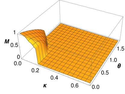
(a)  Magnetization

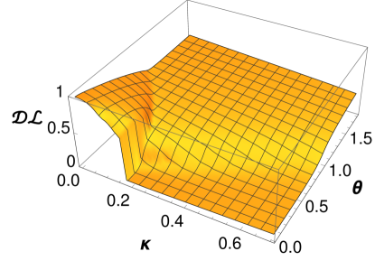
(b)  Domain Length

Figure 3: (a) Magnetization and (b) domain length parameter as functions of $\theta$ and $\kappa$ obtained by temperature downsweeping as explained in the text.

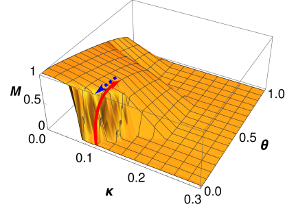
(a)  Magnetization

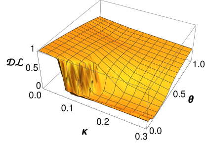
(b)  Domain Length

Figure 4: (a) Magnetization and (b) domain length parameter as functions of $\theta$ and $\kappa$. The initial configuration for all the simulations consists of a flat membrane and randomly oriented pseudo-spins. In (a), we show a heating cycle corresponding to the interaction with a STM tip, see Sec. IV. The continuous red arrow represents the part of the cycle where the temperature is increased and the wrinkled to buckled phase transition occurs, whereas the dashed blue arrow marks the cooling part of the cycle where no transition is found since the system remains buckled.

IV Driving graphene across the rippled to buckled phase transition

In Schoelz et al’s experiments schoelz15 , the floppy rippled membrane undergoes a transition to a rigid buckled state when heated by the STM current. In our model, this may correspond to driving the system across the low temperature first order phase transition seen in Fig. 4 for small values of $\kappa$ and $\theta$. To illustrate this, we set $\kappa=0.1$ and $\theta=0.01$ for all lattice points in our numerical simulations and start with an initially flat membrane and randomly oriented pseudo-spins. We consider $n=35$ rows in a 2d hexagonal lattice, with $N=2100$ atoms. The system reaches a stationary state, which is typically rippled, $M=0$ and ${\cal DL}\simeq 0.1<1/2$.

First, for the sake of simplicity and to understand the basic physical mechanism under the first order transition, we analyze homogeneous heating of the membrane. Second, in order to have a situation closer to the experiments and discuss some more specific details thereof, we consider the case of inhomogeneous heating.

IV.1 Homogeneous heating

Assume that the heat bath temperature felt by the pseudo-spins is the same at all lattice points and varied at a constant rate. The pseudo-spins flip according to the Glauber dynamics given in (3) with the instantaneous and externally controlled value of the temperature $\theta(t)$.

Upon heating, the membrane remains rippled with zero magnetization for $\theta\lesssim 0.15$. At about $\theta_{2}=0.15$, the magnetization and the height of the central atom suddenly increase, as shown in Fig. 5. This effect strongly resembles the STM experiments in ref. schoelz15 , where the increase in dissipated power (modeled here with an increase of the temperature of the heat bath to which the system is coupled) promotes a discrete increase in height, that is, a buckling transition.

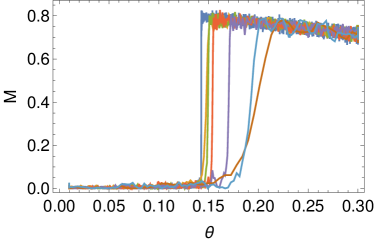
(a)  Magnetization

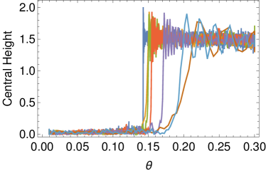
(b)  Central Atom Height

Figure 5: Magnetization and height of the central atom as a function of temperature, upon heating of the system. Different lines correspond to different heating rates. Both the magnetization and the central atom height jump around $\theta_{2}=0.15$, revealing a first-order phase transition in the system. The slower the system is heated, the lower the temperature of the jump. In these simulations the initial and final temperatures are $\theta_{0}=0.01$ and $\theta_{f}=0.3$, respectively. The system is heated with a constant rate, $\theta(t)=\theta_{0}+rt$, and the different lines correspond to rates (from left to right): $3\times 10^{-5}$, $3\times 10^{-4}$, $4\times 10^{-4}$, $6\times 10^{-4}$, $10^{-3}$, $3\times 10^{-3}$, $6\times 10^{-3}$.

The temperature at which the transition occurs depends on the heating rate. For the slowest rates, the jump is almost vertical and takes place at $\theta\simeq 0.15$. For faster rates, the transition is softer and happens for a slightly higher temperature, up to $\theta\simeq 0.20$ for the values considered in Fig. 5. The physical image is the following: a very slow, almost quasi-static, process leads to a sharp transition at the temperature at which the flat membrane becomes unstable. If heating is faster, the system remains in the unstable flat configuration for a certain time and is hindered from finding the “path” to the true thermodynamic equilibrium.

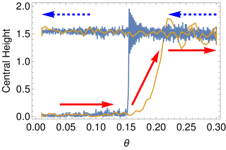
Figure 6: Height of the central atom as a function of the temperature for two heating/cooling cycles, the leftmost and rightmost lines correspond with the slowest and fastest rates of temperature variation in Fig. 5, respectively. The solid arrows and the dashed ones mark the heating and cooling part of the cycle respectively, analogously to the arrows present in Fig. 4. When cooled, the system remains buckled for $\theta<0.15$, which shows that the flat rippled membrane configuration in the low temperature region is metastable.

Finally, in Fig. 6, we present simulations in which the temperature is first increased, until the membrane buckles, and the system is subsequently cooled down to the initial low temperature. Interestingly, we observe that the system remains buckled when the temperature is lowered. This hysteretic behavior is a numerical proof of the metastability of the initial wrinkled configuration for low temperatures and thus is consistent with Fig. 3. The final state resembles the “rigid” states that are reached in STM experiments for large enough currents schoelz15 .

IV.2 Inhomogeneous heating

In STM experiments, the graphene sample is locally heated. We model this by an inhomogeneous temperature profile of a circular membrane of radius $R=1/2$ (clamped at the boundary) inscribed in the unit square. Throughout this section, $\bm{r}$ stands for any point in the circle, $0\leq r\leq R$, with $r=|\bm{r}|$. Energy is injected at the membrane center and the temperature is initially homogeneous throughout the sample, $\theta(\bm{r},t=0)=\theta_{0}$. At $t=0$, the heating process starts, and the border of the sample is always kept at room temperature $\theta_{0}$, $\theta(\bm{r},t)|_{r=1/2}=\theta_{0}$.

The space and time temperature profile obeys the heat equation with a source term,

$$\partial_{t}\theta-\alpha\nabla^{2}\theta=q(\bm{r}),\quad q(\bm{r})=Q_{0}\,e^{-r^{2}/a^{2}},$$ (12)

Note that we are using dimensionless variables, so that the thermal diffusivity $\alpha$ and the energy source from the STM tip $q$ are measured in the units introduced in the previous sections (the dimensions of $\alpha$ and $q$ are $\text{length}^{2}/\text{time}$ and $\text{energy}/\text{time}$, respectively). The source term has radial symmetry and exhibits a Gaussian decay from its maximum value $Q_{0}$ over a characteristic length $a$ (in dimensional units, $a$ is a few angstroms Chen-book ). Note that, for fixed values of $a$ and $\alpha$, the total injected power is proportional to $Q_{0}$. Therefore, we can consider that $Q_{0}\propto IV$ in the STM experiments, where $I$ is the tunneling current and $V$ the voltage bias between the tip and the sample. Interestingly, the same lateral decay of the injected power has been used in other experimental situations, see for instance ref. acs10fau for the study of the thermal conductivity of a graphene membrane excited by a laser.

We seek stationary solutions of the heat equation with radial symmetry, $\theta(r,t)=\theta_{s}(r)$, which obey

$$\nabla^{2}\theta_{s}+\frac{Q_{0}}{\alpha}\,e^{-r^{2}/a^{2}}=0,\\$$ (13a)

$$\theta_{s}(r=R)=\theta_{0},\quad\lim_{r\to 0}|\partial_{r}\theta_{s}(r)|<\infty.$$ (13b)

Equation (13) is solved along the same lines as in ref. acs10fau , with the result

$$\theta_{s}(r)=\theta_{0}+\frac{\Delta\theta}{2}\int_{r/a}^{R/a}dx\,\frac{1-e^{-x^{2}}}{x},\quad\Delta\theta=\frac{Q_{0}a^{2}}{\alpha}.$$ (14)

We plot this stationary temperature profile for several values of $\Delta\theta$ in Fig. 7. We do not consider the transitory decay of the temperature profile to this steady solution, since graphene is a very good thermal conductor acs10fau . Thus, we expect the time scale for the decay to this steady profile to be much shorter than those associated to the increase or the decrease of the voltage bias in the STM experiments. In any case, we would like to stress that taking into account the transient to the stationary state does not alter our conclusions.

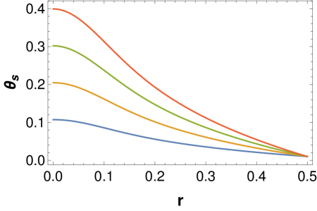
Figure 7: From bottom to top, steady temperature profiles for $\Delta\theta=0.1$, $0.2$, $0.3$, $0.4$.

The STM tip also has an electrostatic interaction with the sample, which is included in our model by adding an external-field term $\Delta{\cal H}$ to the Hamiltonian (1),

$$\Delta{\cal H}=-\sum_{ij}h_{ij}\sigma_{ij}.$$ (15)

Note that the external field breaks the up-down symmetry of the pseudospins, which gives rise to a preferred sign of the curvature in Eq. (9). In ref. schoelz15 , the field $h_{ij}$ decays exponentially from the center of the tip over a characteristic length of a few hundreds of the graphene lattice constant, which is consistent with the long-range character of the electrostatic interaction. In our work, we consider samples with $1650$ atoms inside the circle of unit diameter. For such small samples, the field experiences almost no decay and, therefore, we simply take $h_{ij}=h$, independent of $(i,j)$. Since the strength of the electrostatic interaction increases with the applied bias $V$, we identify $h$ with $V$. Thus, the current is $I=\Delta\theta/V$ and the width of the source term, $a$, is three lattice constants in our simulations. For the sake of clarity, we sum up the key parameters of the model that control the behaviour showed in the simulations in Table 1.

Table 1: Main parameters controlling the behavior of the system in the inhomogeneous heating process, for an applied bias $V$ and a tunneling current $I$ spread over a region of characteristic length $a$, as expressed by Eqs. (12)-(15).

Parameter	Role	Controlling
$\kappa$	Pseudospins’ antiferro interaction	Lower critical temperature $\theta_{2}$, the system buckles for $\theta>\theta_{2}$.
$\Delta\theta\propto IVa^{2}$	Strength of the Joule effect	Temperature at the center of the sample: should be larger than $\theta_{2}$ to induce buckling.
$h$	Strength of the tip-sample electrostatic interaction	Sign of the curvature (breaks up-down symmetry).

To mimic the experimental procedure in ref. schoelz15 , we fix $I$ in each simulation, increase $V$ at a certain constant rate and track the height of the central atom, see Fig. 8. In this way, we are driving the system in the parameter region where there is a first order phase transition as described in the previous section. Except for not having averaged the oscillations in our numerical results, the behavior displayed in Fig. 8 is completely analogous to that observed in ref. schoelz15 , see Fig. 1. For small $I$, the increase in $V$ produces a reversible pulling that increases the global magnetization and the height of the central atom but does not produce overall buckling. Here, reversible means that if the voltage is decreased back to zero from its maximum value, the same curves are swept. This notwithstanding, once $I$ reaches a certain critical value, non-reversible buckling appears (upper-curve): the membrane remains buckled when the voltage is decreased back to zero.

In the STM experiments, the buckling (when it occurs) comprises two steps: apart from the large jump in height at a certain value of the voltage $V_{c}$, there appears a smaller “bump” in height at a smaller voltage $V_{1}<V_{c}$. Interestingly, even this fine detail of the experimental results is reproduced by our model without having to assume a jump in the correlation length $\xi$ as in ref. schoelz15 . As energy is injected, first the maximum of the temperature profile (at the center $r=0$) exceeds the critical value $\theta_{2}\simeq 0.15$ at $V\simeq V_{1}\simeq 0.025$ and this brings about the small height bump observed in Fig. 8 between $V=0.025$ and $V$=0.035. Second, as the voltage bias is further increased to $V_{c}>V_{1}$, there is a large enough region of the system in which the temperature is above $\theta_{2}$, which makes the system buckle.

In the considered range of $V$, $0\leq V\leq 0.06$, heating ($I\neq 0$) is absolutely necessary to produce membrane buckling because the external field is not strong enough by itself. However, if we further raise $V$, it would reach a value at which the system buckles even without heating ($I=0$). Therefore, our model may also be useful to investigate the buckling phenomena observed when strong electrostatic forces are applied, as in refs. lin12 ; svensson11 .

It is worth stressing some further aspects of our numerical results in Fig. 8. First, we increase the voltage at a specific rate and, therefore, different curves are obtained for different rates. Of course, a rate-independent equilibrium curve is obtained if the voltage is increased slowly enough, that is, quasi-statically. Second, our numerical results show some time oscillations. Therefore, the present model allows us to resolve the time evolution of the membrane over a finer scale than that of the currently available experimental results, which are time-averaged.

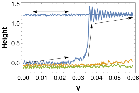
Figure 8: Central atom height vs. voltage bias $V$. The simulations have been conducted in a circular membrane having $N=1650$ sites. From top to bottom, the lines correspond to tunneling currents $I=\Delta\theta/V=1$, $2$, and $6$. The voltage $V$ increases at a constant rate from $0$ to $V_{\max}$ in steps $V_{\max}/250$, during a total time $t_{total}=250$. For clarity, we have shifted downwards the two lowest curves. The curve for $I=6$ exhibits a small bump around $V\simeq 0.025$, which coincides with the maximum of $\theta_{s}$ reaching $0.15$. Once we have reached $V_{\max}$ for $I=6$, we decrease back the voltage to 0 and then height follows the almost flat upper curve. This shows that the jump at $V\simeq 0.035$ is irreversible.

V Discussion

Our spin-membrane model exhibits a first order phase transition from rippled-flat to buckled membrane for appropriately small values of the non-dimensional temperature and spin-spin coupling. The main parameter to be fixed is $\kappa$, that is, the strength of the antiferromagnetic pseudo-spin interaction. Once $\kappa$ has been chosen in the range where the low-temperature first order phase transition is present, it also determines the temperature $\theta_{2}$ above which the membrane buckles. The additional quantities controlling the system behavior are $I$ and $V$, which govern the strength of the Joule effect that heats the membrane, so that the temperature $\theta>\theta_{2}$, and makes it buckle. Conversely, the characteristic length $a$ (which estimates the radius of interaction between the STM tip and the sample) does not play a key role: changing its value only shifts the range of $V$ and $I$ over which driving through the transition is observed.

Membrane buckling arises from the long range interaction among spins induced by the spin-membrane coupling and the metastable state of a flat membrane with ripples stems from the short-range antiferromagnetic spin-spin coupling. To model the results of Schoelz et al’s experiments, we need to drive the system through the first order phase transition by an appropriate control of temperature and the electrostatic interaction between the STM tip and the graphene membrane.

Control of a homogeneous bath temperature induces irreversible buckling but the connection between the parameters of this process and those in the STM experiment is not transparent. Moreover, the STM should heat inhomogeneously the sample. Therefore, we have assumed that the bath temperature adopts the inhomogeneous profile that solves the heat equation with a Gaussian source term. Furthermore, we have introduced an external field term in the spin energy that mimics STM electrostatic force. The latter breaks the spin up-down symmetry which, in turn (via the spin-membrane coupling), breaks the up-down symmetry of the vertical membrane displacements.

The combination of the two above mechanisms produces numerical results that contain every feature of STM buckling experiments, including the existence of a critical value of the current. Our numerical results strongly suggest that both the electrostatic force and heat dissipation are playing a role in the buckling phenomenon observed in ref. schoelz15 . In addition, our spin-membrane model improves that in ref. schoelz15 because it explicitly shows the membrane ripples and it does not need to change the sign of the spin-spin coupling to induce buckling.

There are some hurdles that need to be overcome before finding a microscopic model closer to first principles that explains STM induced buckling of graphene membranes. Firstly, as experiments become more accurate, they may allow for a better definition of all parameters in mesoscopic models, improving the current physical understanding of graphene rippling. Secondly, starting from an electron-phonon Hamiltonian for a suspended graphene sheet, it is possible to derive stationary saddle-point equations for vertical displacements coupled to some auxiliary fields gui14 . From these equations, critical temperatures below which there is buckling can be found ByR16 . These results are qualitatively similar to those found with our spin-membrane model. It seems worth investigating modeling the interaction between the graphene membrane and the STM tip at the level of saddle-point equations. Then some inhomogeneous heating program similar to that in the present paper could be used to explain Schoelz et al’s experiments from “first principles”.

Finally, note that the buckling transition has been also observed in experiments in which only an electrostatic force is applied to the sample, with no energy injection. Our model can also explain this effect, since the external field term favors that the spins have a well-defined sign, that is, that the sign of the membrane curvature is well-defined. In this respect, a detailed experimental study of buckling in graphene, in which both the temperature (via an energy injection mechanism) and the electrostatic force can be independently changed, would greatly improve our insight into the internal interactions that govern buckling.

- (1) J. C. Meyer, A. K. Geim, M. I. Katsnelson, K. S. Novoselov, T. J. Booth, and S. Roth, The structure of suspended graphene sheets. Nature 446, 60-63 (2007).
- (2) N. D. Mermin, Crystalline order in two dimensions, Phys. Rev. 176, 250-254 (1968). Errata in Phys. Rev. B 20, 4762 (1979) and Phys. Rev. B 74, 149902E (2006).
- (3) A. Fasolino, J. H. Los, and M. I. Katsnelson, Intrinsic ripples in graphene. Nature Materials 6, 858-861 (2007).
- (4) N. Abedpour, M. Neek-Amal, R. Asgari, F. Shahbazi, N. Nafari and M. R. Tabar, Roughness of undoped graphene and its short-range induced gauge field. Phys. Rev. B 76, 195407 (2007).
- (5) E. A. Kim and A. H. Castro Neto, Graphene as an electronic membrane. Europhys. Lett. 84, 57007 (2008).
- (6) D. Gazit, Theory of the spontaneous buckling of doped graphene. Phys. Rev. B 79, 113411 (2009).
- (7) P. San-Jose, J. Gonzalez, and F. Guinea, Electron-induced rippling in graphene. Phys. Rev. Lett. 106, 045502 (2011).
- (8) F. Guinea, P. Le Doussal, and K. J. Wiese, Collective excitations in a large- model for graphene. Phys. Rev. B 89, 125428 (2014).
- (9) J. González, Rippling transition from electron-induced condensation of curvature field in graphene. Phys. Rev. B 90, 165402 (2014).
- (10) L. L. Bonilla and M. Ruiz-García, Critical temperature and radius for buckling in graphene, Phys. Rev. B 93, 115407 (2016).
- (11) L. L. Bonilla, A. Carpio, A. Prados and R. R. Rosales, Ripples in a string coupled to Glauber spins. Phys. Rev. E 85, 031125 (2012).
- (12) L. L. Bonilla and A. Carpio, Model of ripples in graphene. Phys. Rev. B 86, 195402 (2012).
- (13) L. L. Bonilla and A. Carpio, Ripples in a graphene membrane coupled to Glauber spins. J. Stat. Mech.: Theor. Exp. P09015 (2012).
- (14) M. Ruiz-Garcia, L. L. Bonilla, and A. Prados, Ripples in hexagonal lattices of atoms coupled to Glauber spins. J. Stat. Mech.: Theor. Exp. P05015 (2015).
- (15) J. K. Schoelz, P. Xu, V. Meunier, P. Kumar, M. Neek-Amal, P. M. Thibado and F. M. Peeters, Graphene ripples as a realization of a two-dimensional Ising model: A scanning tunneling microscope study. Phys. Rev. B 91, 045413 (2015).
- (16) U. Bangert, M. H. Gass, A. L. Bleloch, R. R. Nair, and A. K. Geim, Manifestation of ripples in free-standing graphene in lattice images obtained in an aberration-corrected scanning transmission electron microscope, Physica status solidi (a) 206 1117 (2009).
- (17) F. Guinea, B. Horovitz and P. Le Doussal, Gauge field induced by ripples in graphene, Phys. Rev. B 77 205421 (2008).
- (18) M. I. Katsnelson and A. K. Geim, Electron scattering on microscopic corrugations in graphene, Phil. Trans. R. Soc. A 366 195 (2008).
- (19) H. S. Seung, D. R. Nelson, Defects in flexible membranes with crystalline order. Phys. Rev. A 38, 1005-1018 (1988).
- (20) C. Carraro, D. R. Nelson, Grain-boundary buckling and spin-glass models of disorder in membranes. Phys. Rev. E 48, 3082-3090 (1993).
- (21) O. Lehtinen, S. Kurasch, A. V. Krasheninnikov, U. Kaiser, Atomic scale study of the life cycle of a dislocation in graphene from birth to annihilation. Nature Commun. 4, 2098 (2013).
- (22) J. Kotakoski, F.R. Eder, J. C. Meyer, Atomic structure and energetics of large vacancies in graphene. Phys. Rev. B 89, 201406(R) (2014).
- (23) A. W. Robertson, K. He, A. I. Kirkland, J. W. Warner, Inflating Graphene with Atomic Scale Blisters. Nano Lett. 14, 908-914 (2014).
- (24) L. L. Bonilla, A. Carpio, C. Gong, and J.H. Warner, Measuring strain and rotation fields at the dislocation core in graphene. Phys. Rev. B 92, 155417 (2015).
- (25) N. Lindahl, D. Midtvedt, J. Svensson, O. A. Nerushev, N. Lindvall, A. Isacsson, and E. E. Campbell, Determination of the Bending Rigidity of Graphene via Electrostatic Actuation of Buckled Membranes. Nano Letters 12, 3526-3531 (2012).
- (26) J. Svensson, N. Lindahl, H. Yun, M. Seo, D. Midtvedt, Y. Tarakanov, N. Lindvall, O. Nerushev, J. Kinaret, S.-W. Lee, and E. E. B. Campbell, Carbon nanotube field effect transistors with suspended graphene gates. Nano Letters 11, 3569-3575 (2011).
- (27) P. Xu, M. Neek-Amal, S.D. Barber, J. K. Schoelz, M. L. Ackerman, P. M. Thibado, A. Sadeghi and F.M. Peeters, Unusual ultra-low-frequency fluctuations in freestanding graphene. Nature Commun. 5, 3720 (2014).
- (28) M. Neek-Amal, P. Xu, J. K. Schoelz, M.L. Ackerman, S.D. Barber, P.M. Thibado, A. Sadeghi and F.M. Peeters, Thermal mirror buckling in freestanding graphene locally controlled by scanning tunnelling microscopy. Nature Commun. 5, 4962 (2014)
- (29) M.L. Ackerman, P. Kumar, M. Neek-Amal, P.M. Thibado, F.M. Peeters and S. Singh, Anomalous Dynamical Behavior of Freestanding Graphene Membranes. Phys. Rev. Lett. 117, 126801 (2016)
- (30) A. Prados, L. L. Bonilla and A. Carpio, Phase transitions in a mechanical system coupled to Ising spins, J. Stat. Mech.: Theor. Exp. P06016 (2010).
- (31) L. L. Bonilla, A. Prados and A. Carpio, Nonequilibrium dynamics of a fast oscillator coupled to Glauber spins, J. Stat. Mech.: Theor. Exp. P09019 (2010).
- (32) Y. Mao, and W. L. Wang, D. Wei, E. Kaxiras, and J. G. Sodroski, Graphene structures at an extreme degree of buckling, ACS Nano. 5, 1395 (2011).
- (33) A. O’Hare, F. V. Kursmartsev and K. I. Kugel, A Stable ”Flat” Form of Two-Dimensional Crystals: Could Graphene, Silicene, Germanene Be Minigap Semiconductors?, Nano Lett. 12, 1045 (2012).
- (34) E. Guitter, F. David, S. Leibler, and L. Peliti, Crumpling and Buckling Transitions in Polymerized Membranes. Phys. Rev. Lett. 61, 2949-2952 (1988).
- (35) R. J. Glauber, Time-Dependent Statistics of the Ising Model, J. Math. Phys. 4, 294 (1963).
- (36) C. J. Chen, Introduction to Scanning Tunneling Microscopy (Oxford University Press, New York, 1993).
- (37) C. Faugeras, B. Faugeras, M. Orlita, M. Potemski, R. R. Nair and A. K. Geim, Thermal Conductivity of Graphene in Corbino Membrane Geometry, ACS Nano 4, 1889 (2010).