Appendix

Abstract

Importance sampling is widely used in machine learning and statistics, but its power is limited by the restriction of using simple proposals for which the importance weights can be tractably calculated. We address this problem by studying black-box importance sampling methods that calculate importance weights for samples generated from any unknown proposal or black-box mechanism. Our method allows us to use better and richer proposals to solve difficult problems, and (somewhat counter-intuitively) also has the additional benefit of improving the estimation accuracy beyond typical importance sampling. Both theoretical and empirical analyses are provided.

 

Black-Box Importance Sampling

 

Qiang Liu                        Jason D. Lee Dartmouth College                        University of South California

1 Introduction

Efficient Monte Carlo methods are workhorses for modern Bayesian statistics and machine learning. Importance sampling (IS) and Markov chain Monte Carlo (MCMC) are two fundamental tools widely used when it is intractable to draw exact samples from the underlying distribution $p(x)$. IS uses an simple proposal distribution $q(x)$ to draw a sample $\{x_{i}\}$, and attaches it with a set of importance weights that are proportional to the probability ratio $p(x_{i})/q(x_{i})$. MCMC methods, on the other hand, rely on simulating Markov chains whose equilibrium distribution matches the target distribution.

Unfortunately, both importance sampling (IS) and MCMC have their own critical weaknesses. IS heavily relies on a good proposal $q(x)$ that closely matches the target distribution $p(x)$ to obtain accurate estimates. However, it is critically challenging, or even impossible, to design good proposals for high dimensional complex target distributions, given the restriction of using simple proposals. Therefore, alternative methods that do not require to calculating proposal probabilities would greatly enhance the powerful of IS, yielding efficient solutions for difficulty problems.

On the other hand, MCMC approximates the target distribution with an (often complex) distribution simulated from a large number of steps of Markov transitions, and has been widely used to solve complex problems. However, MCMC has a long-standing difficulty accessing its convergence, and one may get absurdly wrong results when using non-convergent results (e.g., Morris et al., 1996). In addition, the computational cost of MCMC becomes critically expensive when the number of data instances is very large (a.k.a. the big data setting). A number of approximate versions of MCMC have been developed recently to deal with the big data issue (e.g., Welling and Teh, 2011; Alquier et al., 2016), but these methods usually no longer converge to the correct stationary distribution.

Motivated by combining the advantages of IS and MCMC, we study black-box importance sampling methods that can calculate importance weights for any given sample $\{x_{i}\}_{i=1}^{n}$ generated from arbitrary, unknown black-box mechanisms. Such methods allow us to use highly complex proposals that closely match the target distribution, without worrying about the computational tractability of the typical importance weights.

Interestingly, the black-box methods, despite using no information of the proposal distribution, can actually give better estimation accuracy than the typical importance sampling that leverages the proposal information. This appears to be a paradox (using less information yet getting better results), but is consistent with the arguments of O’Hagan (1987) that “Monte Carlo (that uses the proposal information) is fundamentally unsound” for violating the Likelihood Principle, and the interesting results of Henmi et al. (2007); Delyon and Portier (2014) that certain types of approximate versions of IS weights reduce the variance over exact IS weights.

As an example of application, we apply black-box importance weights to samples simulated by a number of short Markov chains, in which MCMC helps provide a complex proposal that are “crudely” closely to the target distribution, and the black-box weights further refine the result. In this way, we obtain consistent estimators even from un-convergent MCMC results, or approximate MCMC transitions that appear commonly in big data settings.

Beyond MCMC, black-box IS can be used to refine many other approximation methods related to complex generation mechanisms, including variational inference with complex proposals (e.g., Rezende and Mohamed, 2015), bootstrapping (Efron, 2012) and perturb-and-MAP methods (Hazan et al., 2013; Papandreou and Yuille, 2011). Further, we envision our method can find more applications in many areas where importance sampling or variance reduction plays an importance role, such as probabilistic inference in graphical model (e.g., Liu et al., 2015), variance reduction for variational inference (e.g., Wang et al., 2013; Ranganath et al., 2014) and policy gradient (e.g., Greensmith et al., 2004), covariance shift in transfer learning (e.g., Sugiyama et al., 2008), off-policy reinforcement learning (e.g., Li et al., 2015), and stochastic optimization (e.g., Zhao and Zhang, 2015).

Our black-box importance weights are calculated by a convex quadratic optimization, based on minimizing a recently proposed kernelized Stein discrepancy that measures the goodness of a sample fit with an unnormalized distribution (Oates et al., 2017; Chwialkowski et al., 2016; Liu et al., 2016); this makes our method widely applicable for unnormalized distributions that widely appear in Bayesian statistics and machine learning.

Related Works

Our method is closely related to Briol et al. (2015a, b); Oates et al. (2017), which combine Stein’s identity with Bayesian Monte Carlo (O’Hagan, 1991; Ghahramani and Rasmussen, 2002) and control variates, respectively, and can also be interpreted as a form of importance weights similar to our method. The key difference is that the weights in their method can be negative and are not normalized to sum to one, while our approach explicitly optimizes the weights in the probability simplex, which helps provide more stable practical results as we illustrate both theoretically and empirically in our work. We provide a more throughout discussion in Section 3.3.

An alternative approach for black-box weights is to directly approximate the underlying proposal distribution $q$ with an estimator $\hat{q}$ and use the corresponding ratio $p(x)/\hat{q}(x)$ as the importance weight. Henmi et al. (2007); Delyon and Portier (2014) showed that certain types of approximation $\hat{q}$ can improve, rather than deteriorate, the performance compared with the weight with the exact $q$. However, the method by Henmi et al. (2007) is not widely applicable since it requires to solve a maximum likelihood estimator in a parametric family that include the proposal distribution; Delyon and Portier (2014) uses a kernel density estimator for $q$ and tends to give unstable empirical results as we show in our experiments. Related to this, there is a literature in semi-supervised learning for covariance shifts (e.g., Sugiyama and Kawanabe, 2012) that estimates the density ratio $p(x)/q(x)$ given two samples $\{x_{i}\}\sim p$ and $\{y_{i}\}\sim q$, when both $p$ and $q$ are unknown.

There are also other directions where the advantages of IS and MCMC can be combined, including adaptive importance sampling (e.g., Martino et al., ; Botev et al., 2013; Beaujean and Caldwell, 2013; Yuan et al., 2013, to only name a few), and sequential Monte Carlo (e.g., Smith et al., 2013; Robert and Casella, 2013; Neal, 2001). The black-box techniques can be combined with these methods to obtain more powerful, adaptive methods.

Preliminary and Notation

Let $k(x,x^{\prime})\colon\mathcal{X}\times\mathcal{X}\to\mathbb{R}$ be a positive definite kernel; we denote by $k(x,\cdot)$ the one-variable function for each fixed $x$. The reproducing kernel Hilbert space (RKHS) $\mathcal{H}$ of $k(x,x^{\prime})$ is the closure of linear span $\{f\colon f=\sum_{i=1}^{m}a_{i}k(x,x_{i}),~{}~{}~{}a_{i}\in\mathbb{R},~{}~{}m\in\mathbb{N},~{}x_{i}\in\mathcal{X}\}$, equipped with an inner product $\langle f,~{}g\rangle_{\mathcal{H}}=\sum_{ij}a_{i}b_{j}k(x_{i},x_{j})$ for $f=\sum_{i=1}^{m}a_{i}k(x,x_{i})$ and $g=\sum_{i}b_{i}k(x,x_{i})$. One can verify that such $\mathcal{H}$ has a reproducing property in that $f=\langle f,~{}k(x,\cdot)\rangle_{\mathcal{H}}$. We use ${\mathcal{O}}(\cdot)$ for the Big O in probability notation.

2 Background: Kernelized Stein Discrepancy

We give a brief introduction to Stein’s identity and kernelized Stein discrepancy (KSD) (Liu et al., 2016; Oates et al., 2017; Chwialkowski et al., 2016) which forms the foundation of our method.

Let $p(x)$ be a continuously differentiable (also called smooth) density supported on $\mathcal{X}\subseteq\mathbb{R}^{d}$. We say that a smooth function $f(x)$ is in the Stein class of $p(x)$ if

$$\int_{\mathcal{X}}\nabla_{x}(p(x)f(x))dx=0,$$ (1)

which can be implied by a zero boundary condition $p(x)f(x)=0$, $\forall x\in\partial\mathcal{X}$ when $\mathcal{X}$ is compact, or $\lim_{||x||\to\infty}f(x)p(x)=0$ when $\mathcal{X}=\mathbb{R}^{d}$. For $f(x)$ in the Stein class of $p(x)$, Stein’s identity shows

$$\begin{split}&\mathbb{E}_{x\sim p}[{\boldsymbol{s}}_{p}(x)f(x)+\nabla_{x}f(x)]=0,\\ &\text{where}~{}~{}~{}~{}~{}{\boldsymbol{s}}_{p}(x)=\nabla_{x}\log p(x),\end{split}$$ (2)

which is in fact a direct rewrite of (1) using the product rule of derivatives. We call ${\boldsymbol{s}}_{p}(x)\coloneqq\nabla_{x}\log p(x)$ the score function of $p(x)$. Note that calculating ${\boldsymbol{s}}_{p}(x)$ does not depend on the normalization constant in $p(x)$, that is, when $p(x)=f(x)/Z$ where $Z$ is the normalization constant and is often critical difficult to calculate, we have ${\boldsymbol{s}}_{p}(x)=\nabla_{x}\log f(x)$, independent of $Z$. This property makes Stein’s identity a powerful practical tool for handling unnormalized distributions that widely appear in machine learning and statistics.

We can “kernelize” Stein’s identity with a smooth positive definite kernel $k(x,x^{\prime})$ for which $k(x,x^{\prime})$ is in the Stein class of $p(x)$ for each fixed $x^{\prime}\in\mathcal{X}$ (we say such $k(x,x^{\prime})$ is in the Stein class of $p$ in this case). By first applying (2) on $k(x,x^{\prime})$ with fixed $x^{\prime}$ and subsequently with fixed $x$, we can get the following kernelized versions of Stein’s identity:

$$\mathbb{E}_{x\sim p}\big{[}{k_{p}}(x,x^{\prime})\big{]}=0,~{}~{}~{}~{}\forall x^{\prime}\in\mathcal{X},$$ (3)

where $x,x^{\prime}$ are i.i.d. drawn from $p$ and ${k_{p}}(x,x^{\prime})$ is a new kernel function defined via

$${k_{p}}(x,x^{\prime})={\boldsymbol{s}}_{p}(x)^{\top}k(x,x^{\prime}){\boldsymbol{s}}_{p}(x^{\prime})+{\boldsymbol{s}}_{p}(x)^{\top}\nabla_{x^{\prime}}k(x,x^{\prime})$$

$$~{}~{}~{}~{}~{}+{\boldsymbol{s}}_{p}(x^{\prime})^{\top}\nabla_{x}k(x,x^{\prime})+\mathrm{trace}(\nabla_{x,x^{\prime}}k(x,x^{\prime})).$$ (4)

See Theorem 3.5 of Liu et al. (2016). (3) suggests that $p(x)$ is an eigenfunction of kernel ${k_{p}}(x,x^{\prime})$ with zero eigenvalue. In fact, let ${\mathcal{H}_{p}}$ be the RKHS related to ${k_{p}}(x,x^{\prime})$, then all the functions $h(x)$ in ${\mathcal{H}_{p}}$ are orthogonal to $p(x)$ in that $\mathbb{E}_{p}[h(x)]=0$. Such ${\mathcal{H}_{p}}$ were first studied in Oates et al. (2017), in which it was used to define an infinite dimensional control variate for variance reduction. We remark that ${k_{p}}(x,x^{\prime})$ can be easily calculated with given $k(x,x^{\prime})$ and ${\boldsymbol{s}}_{p}(x)$, even when $p(x)$ is unnormalized.

If we now replace the expectation $\mathbb{E}_{p}[\cdot]$ in (3) with $\mathbb{E}_{q}[\cdot]$ of a different smooth density $q(x)$ supported on $\mathcal{X}$, (3) would not equal zero; instead, it gives a non-negative discrepancy measure of $p$ and $q$:

$$\mathbb{S}(q,~{}p)=\mathbb{E}_{x,x^{\prime}\sim q}\big{[}{k_{p}}(x,x^{\prime})\big{]}\geq 0,$$ (5)

where $\mathbb{S}(q,~{}p)$ is always nonnegative because ${k_{p}}(x,x^{\prime})$ can be shown to be positive definite if $k(x,x^{\prime})$ is positive definite (e.g., Liu et al., 2016, Theorem 3.6). In addition, one can further show that $\mathbb{S}(q,~{}p)$ equals zero if and only if $p=q$ once $k(x,x^{\prime})$ is strictly positive definite in certain sense: strictly integrally positive definite in Liu et al. (2016), and $cc$-universal in Chwialkowski et al. (2016); these conditions are satisfied by common kernels such as the RBF kernel $k(x,x^{\prime})=\exp(-\frac{1}{2h^{2}}||x-x^{\prime}||^{2}_{2})$, which is also easily in the Stein class of a smooth density $p(x)$ supported in $\mathcal{X}=\mathbb{R}^{d}$ because of its decaying property.

One can further consider kernel ${k_{p}^{+}}(x,x^{\prime})={k_{p}}(x,x^{\prime})+1$, whose corresponding RKHS ${\mathcal{H}_{p}^{+}}$ consists of functions of form $h(x)+c$ with $h\in{\mathcal{H}_{p}}$ and $c$ is a constant in $\mathbb{R}$. Therefore, ${\mathcal{H}_{p}^{+}}$ includes functions with arbitrary values of mean $\mathbb{E}_{p}h$. Further, Chwialkowski et al. (2016) showed that ${\mathcal{H}_{p}^{+}}$ is dense in $L^{2}(\mathcal{X})$ when $k(x,x^{\prime})$ in $cc$-universal. As a consequence, ${\mathcal{H}_{p}}$ is dense in the subset of $L^{2}(\mathcal{X})$ with zero-mean under $p(x)$, that is, for any $h\in L^{2}(\mathcal{X})$ with $\mathbb{E}_{p}[h(x)]=0$ and any $\epsilon>0$, there exists $h^{\prime}\in{\mathcal{H}_{p}}$ such that $||h-h^{\prime}||_{\infty}\leq\epsilon$.

3 Stein Importance Weights

Let $\{x_{i}\}_{i=1}^{n}$ be a set of points in $\mathbb{R}^{d}$ and we want to find a set of weights $\{w_{i}\}_{i=1}^{n}$, $w_{i}\in\mathbb{R}$, such that the weighted sample $\{x_{i},w_{i}\}_{i=1}^{n}$ closely approximates the target distribution $p(x)$ in the sense that

$$\sum_{i=1}^{n}w_{i}h(x_{i})\approx\mathbb{E}_{p}[h(x)],$$

for general test function $h(x)$. For this purpose, we define an empirical version of the KSD in (5) to measure the discrepancy between $\{x_{i},w_{i}\}_{i=1}^{n}$ and $p(x)$,

$$\mathbb{S}(\{x_{i},w_{i}\},~{}p)=\sum_{i,j=1}^{n}w_{i}w_{j}{k_{p}}(x_{i},x_{j})=\boldsymbol{w}^{\top}\boldsymbol{K}_{p}\boldsymbol{w},$$

where $\boldsymbol{K}_{p}=\{{k_{p}}(x_{i},x_{j})\}_{i,j=1}^{n}$ and $\boldsymbol{w}=\{w_{i}\}_{i=1}^{n}$, and we assume the weights are self normalized, that is, $\sum_{i}w_{i}=1$. We then select the optimal weights by minimizing the discrepancy $\mathbb{S}(\{x_{i},w_{i}\},~{}p)$,

$$\begin{split}\hat{\boldsymbol{w}}=\operatorname*{arg\,min}_{\boldsymbol{w}}\bigg{\{}\boldsymbol{w}^{\top}\boldsymbol{K}_{p}\boldsymbol{w},~{}~{}s.t.~{}~{}\sum_{i=1}^{n}w_{i}=1,~{}~{}~{}w_{i}\geq 0\bigg{\}},\end{split}$$ (6)

where in addition to the normalization constraint $\sum_{i}w_{i}=1$, we also restrict the weights to be non-negative; these two simple constraints have important practical implications as we discuss in the sequel. Note that the optimization in (6) is a convex quadratic programming that can be efficiently solved by off-the-self optimization tools. For example, both mirror descent and Frank Wolfe take $O(n^{2}/\epsilon)$ to find the optimum with $\epsilon$-accuracy. Solving (6) does not require to know how the points $\{x_{i}\}_{i=1}^{n}$ are generated, and hence gives a black-box importance sampling.

Theoretically, minimizing the empirical KSD can be justified by the following bound.

Proposition 3.1.

Let $h(x)$ be a test function and $h-\mathbb{E}_{p}h\in{\mathcal{H}_{p}}$. Assume $\sum_{i=1}^{n}w_{i}=1$, we have

$$|\sum_{i=1}^{n}w_{i}h(x_{i})~{}-~{}\mathbb{E}_{p}h|~{}\leq~{}C_{h}\sqrt{\mathbb{S}(\{x_{i},w_{i}\},~{}p)},$$ (7)

where $C_{h}=||h-\mathbb{E}_{p}h||_{{\mathcal{H}_{p}}},$ which depends on $h$ and $p$, but not on $\{x_{i},w_{i}\}_{i=1}^{n}$.

Remark

i) The condition $h-\mathbb{E}_{p}h\in{\mathcal{H}_{p}}$ is a mild requirement as we discussed in Section 2, because ${\mathcal{H}_{p}}$ is dense in the subset of $L^{2}(\mathcal{X})$ with zero means under $p(x)$ when $k(x,x^{\prime})$ is $cc$-universal (Chwialkowski et al., 2016), for which many commonly used kernels satisfy.

ii) Oates et al. (2017, Theorem 3) has a similar result which does not require $\sum_{i}w_{i}=1$, but has a constant term larger than $C_{h}$ when $\sum_{i}w_{i}=1$ does hold. We propose to enforce $\sum_{i}w_{i}=1$ because it gives exact estimation for constant functions $h(x)=c$, and is common practice for importance sampling (which is referred to as self-normalized importance sampling). In our empirical results, we find that the normalized weights can significantly stabilize the algorithm, especially for high dimensional models.

iii) One can show that the $\mathbb{S}(q,~{}p)$ as defined in (5) can be treated as a maximum mean discrepancy (MMD) between $p$ and $q$, equipped with the ($p$-specific) kernel ${k_{p}}(x,x^{\prime})$. In the light of this, bound (7) is a form of the worse case bounds of the kernel-based quadrature rules (e.g., Chen et al., 2010; Bach, 2015; Huszár and Duvenaud, 2012; Niederreiter, 2010). The use of the special kernel ${k_{p}}(x,x^{\prime})$ allows us to calculate the discrepancy tractably for general unnormalized distributions; this is in contrast with the MMDs with typical kernels which are intractable to calculate due to the need for evaluating the a term related to the expectation of the kernel under distribution $p$.

3.1 Practical Applications

Our method as summarized in Algorithm 1 can be used to refine any sample $\{x_{i}\}_{i=1}^{n}$ generated with arbitrary black-box mechanisms, and allows us to apply importance sampling in cases that are otherwise difficult. As an example, we can generate $\{x_{i}\}_{i=1}^{n}$ by simulating $n$ parallel MCMC chains for $m$ steps, where the length $m$ of the chains can be smaller than what is typically used in MCMC, because it just needs to be large enough to bring the distribution of $\{x_{i}\}_{i=1}^{n}$ “roughly” close to the target distribution. This also makes it easy to parallelize the algorithm compared with running a single long chain. In practice, one may heuristically decide if $m$ is large enough by checking the variance of the estimated weights $\{w_{i}\}_{i=1}^{n}$ (or the effective sample size). One can also simulate $\{x_{i}\}_{i=1}^{n}$ using MCMC with approximate translation kernels as these required for massive datasets (e.g., Welling and Teh, 2011; Alquier et al., 2016), so our method provides a new solution for big data problems.

We should remark that when $\{x_{i}\}_{i=1}^{n}$ is simulated from $n$ independent MCMC initialized from a distribution $q_{0}(x)$, the weight $w_{0}(x)=n^{-1}p(x)/q_{0}(x)$ does provide a valid importance sampling weights in that $\sum_{i}w_{0}(x_{i})h(x_{i})$ gives an unbiased estimator (MacEachern et al., 1999, Theorem 6.1). However, this weight does not update as we run more MCMC steps, and performs poorly in practice.

There are many other cases where black-box IS can find useful. For example, we can simulate $\{x_{i}\}_{i=1}^{n}$ from bootstrapping or perturbed maximum a posteriori (MAP) (Papandreou and Yuille, 2011; Hazan et al., 2013), that is, $x_{i}=\operatorname*{arg\,max}_{x}\tilde{p}(x)$ where $\tilde{p}(x)$ is a perturbed version of $p(x)$, or the bootstrapping likelihood. The idea of using importance weighted bootstrapping to carry out Bayesian calculation has been discussed before (e.g., Efron, 2012), but was limited to simple cases when the bootstrap distribution is computable. Black-box IS can also be used to refine the results of variational inference (e.g., Wainwright and Jordan, 2008), especially for the cases with complex variational proposal distributions (e.g., Rezende and Mohamed, 2015).

Algorithm 1 Stein Importance Sampling

  1. Generate $\{x_{i}\}_{i=1}^{n}$ using any mechanism that is believed to resemble $p(x)$ (e.g., by running $n$ independent MCMC chains for a small number of steps, or using parametric bootstrap).

  2. Calculate importance weights for $\{\hat{w}_{i}\}_{i=1}^{n}$ by (6).

  3. Calculate $\sum_{i}\hat{w}_{i}h(x_{i})$ to approximate $\mathbb{E}_{p}[h]$for test function $h$.

3.2 Convergence Rate

Our procedure does not assume the generation mechanism of $\{x_{i}\}_{i=1}^{n}$, but if $\{x_{i}\}_{i=1}^{n}$ is indeed generated “nicely”, error bounds can be easily established using Proposition 3.1: if there exists a set of “reference” positive normalized weights $\{w^{*}_{i}\}_{i=1}^{n}$ such that $\mathbb{S}(\{x_{i},~{}w_{i}^{*}\},~{}p)={\mathcal{O}}(n^{-\delta})$, then the mean square error of our estimator with weight $\{\hat{w}_{i}\}_{i=1}^{n}$ returned by (6) should also be ${\mathcal{O}}(n^{-\delta})$ by following (6) and (7).

To gain more intuition, assume ${k_{p}}(x,x^{\prime})$ has a set of eigenfunctions $\{\phi_{\ell}(x)\}$ and eigenvalues $\{\lambda_{\ell}\}$ such that ${k_{p}}(x,x^{\prime})=\sum_{\ell}\lambda_{\ell}\phi_{\ell}(x)\phi_{\ell}(x^{\prime})$, then we have

$$|\sum_{i}\hat{w}_{i}h(x_{i})-\mathbb{E}_{p}h|^{2} \leq C_{h}^{2}~{}{\mathbb{S}(\{x_{i},\hat{w}_{i}\},~{}p)}$$

$$=C_{h}^{2}~{}\sum_{\ell}\lambda_{\ell}~{}(\sum_{i}w_{i}\phi_{\ell}(x_{i})-\mathbb{E}_{p}\phi_{\ell})^{2},$$

where $C_{h}=||h-\mathbb{E}_{p}h||_{{\mathcal{H}_{p}}}$ and we used the fact that $\mathbb{E}_{p}\phi_{\ell}=0$ since $\phi_{\ell}\in{\mathcal{H}_{p}}$. Therefore, it is enough to find a set of positive and normalized reference weights whose error on estimating $\mathbb{E}_{p}\phi_{\ell}$ is low. Note that such reference weight does not necessarily need to be practically computable to establish the bound.

As an obvious example, when $\{x_{i}\}_{i=1}^{n}$ is i.i.d. drawn from an (unknown) proposal distribution $q(x)$, the typical importance sampling weight $w^{*}_{i}\propto p(x_{i})/q(x_{i})$ (up to the normalization) can be used as a reference weight to establish an ${\mathcal{O}}(n{}^{-1/2})$ error rate as the typical Monte Carlo methods have.

Theorem 3.2.

Assume $h-\mathbb{E}_{p}h\in{\mathcal{H}_{p}}$ and $\{x_{i}\}_{i=1}^{n}$ is i.i.d. drawn from $q(x)$ with the same support as $p(x)$. Define $w_{*}(x)=p(x)/q(x)$ and assume $\mathbb{E}_{x\sim p}(|w_{*}(x){k_{p}}(x,x)|)<\infty$, and $\mathbb{E}_{\{x,x^{\prime}\}\sim p}[w_{*}(x)w_{*}(x^{\prime}){k_{p}}(x,x^{\prime})^{2}]<\infty$. For $\{\hat{w}_{i}\}_{i=1}^{n}$ defined in (6), we have

$$|\sum_{i=1}^{n}\hat{w}_{i}h(x_{i})-\mathbb{E}_{p}h|={\mathcal{O}}({n^{-1/2}}).$$

Interestingly, it turns out the typical importance weight $w_{*}(x)\propto p(x)/q(x)$ is not the best possible reference weight; better options can be constructed using various variance reduction techniques to give convergence rates better than the typical ${\mathcal{O}}(n^{-1/2})$ rate.

Theorem 3.3.

Assume $\{x_{i}\}_{i=1}^{n}$ is i.i.d. drawn from $q(x)$ and $w_{*}(x)=p(x)/q(x)$. Let $\{\phi_{\ell}\}_{\ell=1}^{\infty}$ be the set of orthogonal eigenfunctions w.r.t. $p(x)$ with eigenvalues $\{\lambda_{\ell}\}_{\ell=1}^{\infty}$. Assume all the following quantities are upper bounded by $M$ uniformly for $\forall x\in\mathcal{X}$: $\sum_{\ell=1}^{\infty}\lambda_{\ell}$, $w_{*}(x)$, $|\phi(x)|$, $\max_{\ell,\ell^{\prime}}\mathrm{var}_{x\sim q}[w_{*}(x)^{2}\phi_{\ell}(x)\phi_{\ell}^{\prime}(x)]$, we have

$$\mathbb{E}_{\boldsymbol{x}\sim q}\big{[}|\sum_{i}\hat{w}_{i}h(x_{i})-\mathbb{E}_{p}h|^{2}\big{]}^{1/2}=\mathcal{O}{\left(n^{-(1+\alpha)/2}\right)},$$

where $\alpha$ is a number that satisfies $0<\alpha\leq 1$ and is decided by the bound $M$ and the decay of the eigenvalues $\mathcal{R}(n)=\sum_{\ell>n}\lambda_{\ell}$ of kernel $k_{p}(x,x^{\prime})$. See Theorem B.5 in Appendix for more details.

The proof of Theorem 3.3 (see Section 2.2 in Appendix) is based on first constructing a set of (possibly negative) reference weights using a control variates method based on the orthogonal basis functions $\{\phi_{\ell}\}$, and then zero out the negative elements and normalize the sum to obtain a set of positive normalized reference weights. This is made possible because the initial reference obtained by control variates is mostly likely positive, since they can be treated as a perturbed version of the typical (positive) importance weights $w_{*}(x)\propto p(x)/q(x)$ as used in Theorem (3.2), where the perturbation is introduced to cancel the estimation error and increase the accuracy. Therefore, zeroing out the negative elements does not have significant impact on the error bound compared with the initial reference weights. This provides a justification on the non-negative constraint, and allows us to construct a set of non-negative reference weights for our proof. The non-negative constraint, also known as the garrote constraint (Breiman, 1995), is also motivated by the empirical observation that it gives more stable results for small sample size $n$ (intuitively, it seems hard to believe that a large negative weight would give improvements when $n$ is small, unless the points $\{x_{i}\}_{i=1}^{n}$ were introduced in a careful way).

The proof of Theorem 3.3 (see Section 2.2 in Appendix) is based on constructing a reference weight using a control variates method based on the orthogonal basis functions $\{\phi_{\ell}\}$. Our constructed reference weights can be treated as a perturbed version of the typical importance weights $w_{*}(x)\propto p(x)/q(x)$ as used in Theorem (3.2), where the perturbation is introduced to cancel the estimation error and increase the accuracy. Since this reference weights concentrate around $w_{*}\propto p(x)/q(x)$ which is positive, we can zero out its negative values without much impact on the error bound. This provides a justification on the non-negative garrote constraint, and allows us to construct a set of non-negative reference weights for our proof.

Similar theoretical analysis can be found in Briol et al. (2015a); Bach (2015). In particular, Briol et al. (2015a) used a similar “reference weight” idea to establish a convergence rate for Bayesian Monte Carlo. The main technical challenge in our proof is to make sure that the reference weight satisfies the non-negative and self-normalization constraints. Section 2.2 in Appendix provides more detailed discussions.

3.3 Other “Super-Efficient” Weights

We review several other types of “supper-efficient” weights that also give better convergence rates than the typical ${\mathcal{O}}(n^{-1/2})$ rate; this includes Bayesian Monte Carlo and the related (linear) control variates method, as well as methods based on density approximation of the proposal distributions, which can be interpreted as multiplicative control variates (Nelson, 1987) that reduce the variance.

Bayesian Monte Carlo and Control Variates

Bayesian Monte Carlo (O’Hagan, 1991; Ghahramani and Rasmussen, 2002) was originally developed to evaluate integrals using Bayesian inference procedure with Gaussian prior, which turns out to be equivalent to a weighted form $\sum_{i}w_{i}h(x_{i})$ with $w_{i}$ being a set of weights independent of the test function $h$; unlike our method, these weights are not normalized to sum to one and can take negative values.

From a RKHS perspective, one can interpret Bayes MC as approximating $\mathbb{E}_{p}[h(x)]$ with $\mathbb{E}_{p}[\hat{h}(x)]$ where $\hat{h}(x)$ is an approximation of $h(x)$ constructed by kernel linear regression based on the data-value pair $\{x_{i},h(x_{i})\}_{i=1}^{n}$. Let $k_{0}(x,x^{\prime})$ be the kernel used in Bayes MC, then one can show that Bayes MC estimate equals $\sum_{i}\hat{w}_{i}h(x_{i})$ with $\hat{\boldsymbol{w}}=[\hat{w}_{i}]_{i=1}^{n}=(\boldsymbol{K}_{0}+\lambda I)^{-1}\boldsymbol{b}$, where $\boldsymbol{K}_{0}=[k_{0}(x_{i},x_{j})]_{ij}$ and $\boldsymbol{b}=[\mathbb{E}_{x\sim p}(k_{0}(x,x_{i}))]_{i=1}^{n}$, and $\lambda$ a regularization coefficient. Equivalently, Bayes MC can be treated as minimizing the maximum mean discrepancy (MMD) between $\{x_{i},w_{i}\}$ and $p$, with a form of

$$\hat{\boldsymbol{w}}=\arg\min_{\boldsymbol{w}}\big{\{}\boldsymbol{w}^{\top}\boldsymbol{K}_{0}\boldsymbol{w}-2\boldsymbol{b}^{\top}\boldsymbol{w}+\lambda||\boldsymbol{w}||_{2}^{2}\big{\}}.$$

One of the main difficulty of Bayesian MC, however, is that it depends on $\boldsymbol{b}=\mathbb{E}_{p}[k_{0}(x,x^{\prime})]$, which can be intractable to calculate for complex $p(x)$.

The control variates method (e.g., Liu, 2008) also relies on a (kernel) linear regressor $\hat{h}(x)$, but estimates $\mathbb{E}_{p}h$ with a bias-correction term $\frac{1}{n}\sum_{i=1}^{n}(h(x_{i})-\hat{h}(x_{i}))+\mathbb{E}_{p}[\hat{h}(x_{i})]$, which can also be rewritten into a weighted form. Note that when $\lambda=0$ and $\boldsymbol{K}_{0}$ is strictly positive definite, the $\hat{h}(x_{i})$ becomes an interpolation of $h(x)$ (i.e., $h(x_{i})=\hat{h}(x_{i})$), and control variates and Bayes MC becomes equivalent. In control variates, one can also use only a subset of the data to estimate $\hat{h}(x)$ and use the remaining data to estimate the expectation of the difference $h(x)-\hat{h}(x)$; this ensures the resulting estimator is unbiased.

Theoretically, the convergence rate of control variates and Bayesian Monte Carlo can both be established to be ${\mathcal{O}}(n^{-(1+\alpha)/2})$, where $\alpha$ depends on how well $\hat{h}(x)$ can approximate $h(x)$; see Oates et al. (2017, 2016); Briol et al. (2015a, b); Bach (2015) for detailed analysis.

Closely related to our work, Oates et al. (2017) and Briol et al. (2015a) proposed to use the Steinalized kernel ${k_{p}^{+}}(x,x^{\prime})={k_{p}}(x,x^{\prime})+1$ in control variates and Bayesian MC, respectively, for which $\boldsymbol{b}=\mathbb{E}_{x\sim p}[{k_{p}^{+}}(x,x^{\prime})]=1$. We can show that their method is equivalent to using the following weight

$$\hat{\boldsymbol{w}}=\operatorname*{arg\,min}_{\boldsymbol{w}}\{\boldsymbol{w}^{\top}\boldsymbol{K}_{p}\boldsymbol{w}+(\sum_{i}w_{i}-1)^{2}+\lambda||w||_{2}^{2}\}.$$

This form is similar to our (6), but does not enforce the non-negative garrote constraint (Breiman, 1995) and replacing the normalization constraint $\sum_{i}w_{i}=1$ with a quadratic regularization with regularization coefficient of one. Here the L2 penalty $\lambda||w||_{2}^{2}$ is necessary for ensuring numerical stability in practice. In our case, it is the non-negative constraint that helps stabilize the optimization problem, without needing to specify a regularization parameter.

Approximating the Proposal Distribution

Another (perhaps less well known) set of methods are based on replacing the importance weight $w_{*}(x)=p(x)/q(x)$ with an approximate version $\tilde{w}(x)=p(x)/\hat{q}(x)$, where $\hat{q}(x)$ is an estimator of proposal density $q(x)$ from $\{x_{i}\}_{i=1}^{n}$. While we may naturally expect that such approximation would decrease the accuracy compared with the typical IS that uses the exact $q(x)$, surprising results (Henmi et al., 2007; Delyon and Portier, 2014) show that in certain cases the approximate weights $\tilde{w}(x)$ actually improve the accuracy. To gain an intuition why this can be the case, observe that we have $\tilde{w}(x)=[p(x)/q(x)]\cdot[q(x)/\hat{q}(x)]$, where the second term $q(x)/\hat{q}(x)$ may acts as a (multiplicative) control variate (Nelson, 1987) which can decrease the variance if it is negatively correlated with the rest parts of the estimator. For asymptotic analysis, it is common to expend multiplicative control variates using Taylor expansion, which reduces it to linear control variates.

In particular, Henmi et al. (2007) showed that when $q(x)$ is embedded in a parametric family $\mathcal{Q}=\{q(x\mid\theta)$, $\theta\in\Theta\}$, replacing $w_{*}(x)$ with the approximate weight $\tilde{w}(x)=p(x)/\hat{q}(x)$, where $\hat{q}$ is the maximum likelihood estimator of $q(x)$ within $\mathcal{Q}$, would guarantee to decrease the asymptotic variance compared with the standard IS. The result in Delyon and Portier (2014) forms a non-parametric counterpart of Henmi et al. (2007), in which it is shown that taking $\hat{q}(x)$ to be a leave-one-out kernel density estimator of $q(x)$ would give super-efficient error rate ${\mathcal{O}}(n^{-(1+\alpha)/2})$ where $\alpha$ is a positive number that depends on the smoothness of $q(x)$ and $p(x)h(x)$.

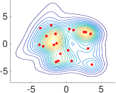
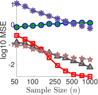
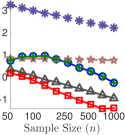
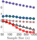
(a) Contour of $p(x)$	(b) $\mathbb{E}(x)$	(c) $\mathbb{E}(x^{2})$	(d) $\mathbb{E}(\cos(\omega x+b))$

Figure 1: Gaussian Mixture Example. (a) The contour of the distribution $p(x)$ that we use; the red dots represent the centers of the mixture components. The sample $\{x_{i}\}$ is i.i.d. drawn from $p(x)$ itself. (b) - (c) The MSE of the different weighting schemes for estimating $\mathbb{E}_{p}h$, when $h(x)$ equals $x$, $x^{2}$, and $\cos(\omega x+b)$, respectively. For $h=\cos(\omega x+b)$ in (d), we draw $\omega\sim\mathcal{N}(0,1)$ and $b\sim\textrm{Uniform}([0,2\pi])$ and average the MSE over $20$ trials.

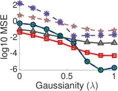
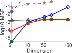
(a) Varying Gaussianity		(b) Varying Dimension

Figure 2: (a) Results on $p(x|\lambda)$ where $\lambda$ indexes the Gaussianity: $p(x|\lambda)$ equals $\mathcal{N}(0,1)$ when $\lambda=1$ and it reduces to the $p(x)$ in Figure 1(a) when $\lambda=0$. (b) Results on standard Gaussian distribution with increasing dimensions. The sample size is fixed to be $n=100$ in both (a) and (b). The MSE is for estimating $\mathbb{E}(x^{2})$.

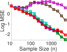
(c) Stein with relaxed $w_{i}\geq-b$ constraint

Figure 3: The result of our method on the $p(x)$ in Figure 1(a) when the non-negative constraint $w_{i}\geq 0$ replaced by a general lower bound $w_{i}\geq-b$ with different values of $b$. The MSE is for estimating $\mathbb{E}(x^{2})$.

4 Experiments

We empirically evaluate our method and compare it with the methods mentioned above, first on an illustrative toy example based on Gaussian mixture, and then on Bayesian probit regression. The methods we tested all have a form of $\sum_{i}w_{i}h(x_{i})$, where the weights $w_{i}$ are decided by one of the following algorithms:

1. Uniform weights $w_{i}=1/n$ (Uniform).

2. Our method that solves (6) (referred as Stein), for which we use RBF kernel $k(x,x^{\prime})=\exp(-\frac{1}{h}||x-x^{\prime}||^{2}_{2})$; the bandwidth $h$ is heuristically chosen to be the median of the pairwise square distance of data $\{x_{i}\}_{i=1}^{n}$ as suggested by Gretton et al. (2012).

3. The control functional method Control Func following the empirical guidance in Oates et al. (2017), which is also equivalent to Bayesian MC with kernel ${k_{p}^{+}}(x,x^{\prime})={k_{p}}(x,x^{\prime})+1$. Note that the weights $\{w_{i}\}$ in this method may be negative and do not necessarily sum to one. We also test a modified version of it $\sum_{i}w_{i}h(x_{i})/\sum_{i}w_{i}$ that normalizes the weights and refer it as Control Func (Normalized). The kernel $k(x,x^{\prime})$ and the bandwidth are taken to be the same as our method. We follow Oates et al. (2017)’s guidance to select that an L2 regularization coefficient to stabilize the algorithm.

4. The kernel density estimator (KDE) based method by Delyon and Portier (2014) (KDE), which uses weights $w_{i}=n^{-1}p(x_{i})/\hat{q}_{i}(x_{i})$, where $\hat{q}_{i}(x)$ is a leave-one-out KDE of form $\hat{q}_{i}(x)=\sum_{j\neq i}k(x,x_{j})/n$. We report the result when using RBF kernel with bandwidth decided by the rule of thumb $h=\hat{\sigma}\big{(}\frac{d2^{d+5}\Gamma(d/2+3)}{(2d+1)n}\big{)}^{1/(4+d)}$, where $\hat{\sigma}$ is the standard deviation of $\{x_{i}\}_{i=1}^{n}$ and $d$ is the dimension of $x$. We also tested the choice of kernel and bandwidth suggested in Delyon and Portier (2014) but did not find consistent improvement. Similar to the case of the control functional method, we also test a self-normalized version of KDE and denote it by KDE (Normalized).

We evaluate these methods by comparing their mean square errors (MSE) for estimating $\mathbb{E}_{p}h$, with $h(x)$ taken to be $x$, $x^{2}$ or $\cos(\omega x+b)$. For $h(x)=\cos(\omega x+b)$, we draw $\omega\sim\mathcal{N}(0,1)$ and $b\sim\textrm{Uniform}([0,2\pi])$ and average the MSE over $20$ random trials.

Gaussian Mixture

We start with a $2$-D Gaussian mixture distribution $p(x)=\sum_{j}\beta_{j}\mathcal{N}(x;~{}\mu_{j},\sigma_{j}^{2})$ with $20$ randomly located mixture components shown in Figure 1(a), and draw $\{x_{i}\}_{i=1}^{n}$ from $p(x)$ itself. The MSEs for estimating $\mathbb{E}_{p}h$ with different $h(x)$ as the sample size $n$ increases are shown in Figure 1(b)-(d), where we generally find that our method tends to perform among the best.

In Figure 2(a), we study the performance of the algorithms on distributions with different Gaussianity, where we replace $p(x)$ with a series of distributions $p(x\mid\lambda)$ whose random variable is $(1-\lambda)x+\lambda\xi$ where $x\sim p$, $\xi\sim\mathcal{N}(0,1)$ and $\lambda\in[0,1]$ controls the Gaussianity of $p(x\mid\lambda)$: it reduces to $p(x)$ when $\lambda=0$ and equals $\mathcal{N}(0,1)$ when $\lambda=1$. We observe that Stein tends to perform the best when the distribution has high non-Gaussianity, but is suboptimal compared with Control Func when the distribution is close to Gaussian.

In Figure 2(b), we consider how the different algorithms scale to high dimensions by setting $p(x)$ to be the standard Gaussian distribution with increasing dimensions. We generally find that our Stein tends to perform among the best under the different settings, expect for low dimensional standard Gaussian under which Control Func performs the best. The self-normalized versions of KDE and Control Func can help to stabilize the algorithm in various cases, for example, KDE (Normalized) significantly improves over KDE in all the cases, and Control Func (Normalized) is significantly better than Control Func in high dimensional cases as shown in Figure 2(b).

Figure 3 shows the performance of our method with the non-negativity constraint ($w_{i}\geq 0$) replaced by $(w_{i}\geq-b)$ where $b$ is a positive number that takes different values. We find that the result of $w_{i}\geq 0$ generally performs the best when $n$ is small (e.g., $n<1000$), but is slightly suboptimal when $n$ is large. Because the stability in the small $n$ case is more practically important than the large $n$ case, given that the absolute difference on MSE would be negligible in the large $n$ region, we think enforcing $w_{i}\geq 0$ is a simple and good practical procedure.

(a) Estimating $\mathbb{E}(x)$	(b) Estimating $\mathbb{E}(x^{2})$

Figure 4: Results of Bayesian probit model with simulated data. We generate $\{x_{i}\}_{i=1}^{n}$ by simulating $n$ parallel chains of stochastic gradient Langevin Dynamics with a mini-batch size of $100$ for $100$-steps. KDE and KDE (Normalized) perform significantly worse in this case, and are not show in the figure.

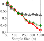
(a) Estimating $\mathbb{E}(x)$	(b) Estimating $\mathbb{E}(x^{2})$

Figure 5: Results of Bayesian probit model on the Covtype dataset. We generate $\{x_{i}\}_{i=1}^{n}$ by simulating $n$ parallel chains of stochastic gradient Langevin Dynamics with a mini-batch size of $100$ for $1000$-steps. The unnormalized Control Func, as well as KDE and KDE (Normalized) perform significantly worse in this case, and are not show in the figure.

Bayesian Probit Model

We consider the Bayesian probit regression model for binary classification. Let $D=\{\chi_{\ell},\zeta_{\ell}\}_{\ell=1}^{N}$ be a set of observed data with feature vector $\chi_{\ell}$ and binary label $\zeta_{\ell}\in\{0,1\}$. The distribution of interest is $p(x)\coloneqq p(D|x)p_{0}(x)$ with

$$p(D|x)=\prod_{\ell=1}^{N}\big{[}\zeta_{\ell}\Phi(x^{\top}\chi_{\ell})+(1-\zeta_{\ell})(1-\Phi(x^{\top}\chi_{\ell}))\big{]},$$

where $\Phi(\cdot)$ is the cumulative distribution function of the standard normal distribution, and $p_{0}(x)=\mathcal{N}(x;0,0.1)$ is the prior.

To test our method, we simulate $\{x_{i}\}_{i=1}^{n}$ by running $n$ parallel chains of stochastic Langevin dynamics (Welling and Teh, 2011). Since this method is an inexact MCMC, its stationary distribution should be different from the target distribution $p(x)$. As a result, directly averaging $\{x_{i}\}_{i=1}^{n}$ with uniform weights (Unif) can give relatively poor results with convergence rate slower than the typical $\O(n^{-1/2})$ rate (see e.g., Teh et al. (2016)). The black-box weights can be used refine the result.

Figure 4 shows the result on a small simulated dataset with $100$ data instances and $10$ features. We can find that Stein and Control Func (Normalized) significantly improve the performance over Unif. Interestingly, we find that the unnormalized Control Func, as well as KDE and KDE (normalized) (not show in the figure) perform significantly worse in this case.

Figure 5 shows the result on the Forest Covtype dataset from the UCI machine learning repository (Bache and Lichman, 2013); it has 54 features, and is reprocessed to get binary labels following Collobert et al. (2002). For our experiment, we take the first 10,000 data points, so that it is feasible to evaluate the ground truth with No-U-Turn Sampler (NUTS) (Hoffman and Gelman, 2014). We again find that Stein and Control Func (Normalized) improves over the uniform weights, and the unnormalized Control Func and KDE and KDE (normalized) again perform significantly worse and are not shown in the figure.

5 Conclusion

We propose a black-box importance sampling method that calculates importance weights without knowing the proposal distribution, which also has the additional benefit of providing variance reduction. We expect our method provides a powerful tool for solving many difficult problems were previously intractable via importance sampling.

This document contains derivations and other supplemental information for “Black-box Importance Sampling”.

Appendix A Kernelized Stein Discrepancy

Proof of Proposition 3.1.

Let $\tilde{h}(x)=h(x)-\mathbb{E}_{p}h$, we have

$$|\sum_{i}w_{i}\tilde{h}(x_{i})| =|\sum_{i}w_{i}\langle\tilde{h},~{}{k_{p}}(\cdot,x_{i})\rangle_{{\mathcal{H}_{p}}}|$$

$$=|\langle\tilde{h},~{}\sum_{i}w_{i}{k_{p}}(\cdot,x_{i})\rangle_{{\mathcal{H}_{p}}}|$$

$$\leq||\tilde{h}||_{{\mathcal{H}_{p}}}\cdot||\sum_{i}w_{i}{k_{p}}(\cdot,x_{i})||_{{\mathcal{H}_{p}}}$$

$$=||\tilde{h}||_{{\mathcal{H}_{p}}}\cdot\sqrt{\mathbb{S}(\{w_{i},x_{i}\},~{}p)}.$$

where we used Cauchy-Schwarz inequality and the fact that $||\sum_{i}w_{i}{k_{p}}(\cdot,x_{i})||_{{\mathcal{H}_{p}}}^{2}=\sum_{ij}w_{i}w_{j}{k_{p}}(x_{i},x_{j})=\mathbb{S}(\{w_{i},x_{i}\},~{}p)$. ∎

Appendix B Convergence Rate

We consider the error rate of our estimator $\sum_{i}\hat{w}_{i}(\boldsymbol{x})h(x_{i})$ with $\{\hat{w}_{i}(\boldsymbol{x})\}$ given by the optimization in (6), under the assumption that $\boldsymbol{x}=\{x_{i}\}_{i=1}^{n}$ is i.i.d. drawn from an (unknown) distribution $q(x)$. Based on the bound in Proposition (3.1), we can establish an error rate ${\mathcal{O}}(n^{-\delta})$ by finding a set of oracle “reference weights” $\{w_{*i}(\boldsymbol{x})\}$, as a function of $\boldsymbol{x}$, such that $\mathbb{S}(\{x_{i},w_{*i}(\boldsymbol{x})\},~{}p)={\mathcal{O}}(n^{-2\delta})$, because

$$|\sum_{i}\hat{w}_{i}(\boldsymbol{x})h(x_{i})-\mathbb{E}_{p}h|\leq C_{h}\cdot\sqrt{\mathbb{S}(\{\hat{w}_{i}(\boldsymbol{x}),x_{i}\},~{}p)}\leq C_{h}\cdot\sqrt{\mathbb{S}(\{w_{*i}(\boldsymbol{x}),x_{i}\},~{}p)}={\mathcal{O}}(n^{-\delta}),$$

where $C_{h}=||h-\mathbb{E}_{p}h||_{{\mathcal{H}_{p}}}$. This idea of using reference weights has been used in Briol et al. (2015a) to study the convergence rate of Bayesian Monte Carlo.

Section B.1 proves the ${\mathcal{O}}(n^{-1/2})$ rate using the typical importance sampling weights as the reference weight. Section B.2 proves a better $\mathchoice{{\scriptstyle\mathcal{O}}}{{\scriptstyle\mathcal{O}}}{{\scriptscriptstyle\mathcal{O}}}{\scalebox{0.7}{$\scriptscriptstyle\mathcal{O}$}}{\left(n^{-1/2}\right)}$ rate by using a reference weight based on a control variates method constructed with an orthogonal basis estimator.

B.1 ${\mathcal{O}}(n^{-1/2})$ Rate

We use the typical importance sampling weight as a reference weight and establish ${\mathcal{O}}(n^{-1/2})$ rate on the error of our estimator.

Assumption B.1.

Assume $p(x)/q(x)>0$ for $\forall x\in\mathcal{X}$ and $\mathbb{E}_{x\sim q}[\big{(}\frac{p(x)}{q(x)}\big{)}^{2}]<\infty$, $\mathbb{E}_{x\sim q}(|\frac{p(x)^{2}}{q(x)^{2}}{k_{p}}(x,x)|)<\infty$, and $\mathbb{E}_{x,x^{\prime}\sim q}\big{[}\big{(}\frac{p(x)p(x^{\prime})}{q(x)q(x^{\prime})}{k_{p}}(x,x^{\prime})\big{)}^{2}\big{]}<\infty$.

Lemma B.2.

Assume $\{x_{i}\}_{i=1}^{n}$ is i.i.d. drawn from $q(x)$

$$w_{i}^{*}=\frac{1}{Z}p(x_{i})/q(x_{i}),~{}~{}~{}Z=\sum_{i}p(x_{i})/q(x_{i}),$$

then under Assumption B.1 we have

$$\mathbb{S}(\{w_{i}^{*},x_{i}\},~{}p)={\mathcal{O}}(n^{-1}).$$

Proof.

Define $v_{i}^{*}(x_{i})=\frac{1}{n}p(x_{i})/q(x_{i})$, and

$$\mathbb{S}(\{v_{i}^{*},x_{i}\},~{}p)=\frac{1}{n^{2}}\sum_{ij}\frac{p(x_{i})}{q(x_{i})}\frac{p(x_{j})}{q(x_{j})}{k_{p}}(x_{i},x_{j}),$$

then $\mathbb{S}(\{v_{i}^{*},x_{i}\},~{}p)$ is a degenerate V-statistic since by (3) we have

$$\mathbb{E}_{x^{\prime}\sim q}[\frac{p(x)}{q(x)}\frac{p(x^{\prime})}{q(x^{\prime})}{k_{p}}(x^{\prime},x^{\prime})]=\frac{p(x)}{q(x)}\mathbb{E}_{x^{\prime}\sim p}[{k_{p}}(x_{i},x_{j})]=0,~{}~{}~{}~{}~{}\forall x\in\mathcal{X}$$

then we have (see e.g., Lee, 1990)

$$\mathbb{S}(\{v_{i}^{*},x_{i}\},~{}p)={\mathcal{O}}(n^{-1}).$$

In addition, note that $\sum_{i=1}^{n}v_{i}^{*}=1+{\mathcal{O}}(n^{-1/2})$, we have

$$\mathbb{S}(\{w_{i}^{*},x_{i}\},~{}p)=\frac{\mathbb{S}(\{v_{i}^{*},x_{i}\},~{}p)}{(\sum_{i}v_{i}^{*})^{2}}={\mathcal{O}}(n^{-1}).$$

∎

Theorem B.3.

Assume $\{x_{i}\}$ is i.i.d. drawn from $q(x)$, and $\{\hat{w}_{i}(\boldsymbol{x})\}$ is given by (6), then under Assumption B.1, we have

$$\sum_{i=1}^{n}\hat{w}_{i}(\boldsymbol{x})h(x_{i})-\mathbb{E}_{p}h={\mathcal{O}}({n^{-1/2}}).$$

Proof.

Simply note that

$$\mathbb{S}(\{\hat{w}_{i},x_{i}\}_{i=1}^{n},~{}p)\leq\mathbb{S}(\{w_{i}^{*},x_{i}\}_{i=1}^{n},~{}p)={\mathcal{O}}({n^{-1}}),$$

and combining with Proposition 3.1 gives the result. ∎

B.2 ${\scriptstyle{\mathcal{O}}}(n^{-1/2})$ Rate

We prove Theorem 3.3 that shows an $\mathchoice{{\scriptstyle\mathcal{O}}}{{\scriptstyle\mathcal{O}}}{{\scriptscriptstyle\mathcal{O}}}{\scalebox{0.7}{$\scriptscriptstyle\mathcal{O}$}}{\left(n^{-1/2}\right)}$ rate for our estimator. Our method is based on constructing a reference weight by using a two-fold control variate method based on the first $L$ orthogonal eigenfunctions $\{\phi_{\ell}\}$ of kernel ${k_{p}}(x,x^{\prime})$.

We first re-state the assumptions made in Theorem 3.3.

Assumption B.4.

1. Assume ${k_{p}}(x,x^{\prime})$ has the following eigen-decomposition

$${k_{p}}(x,x^{\prime})=\sum_{\ell}\lambda_{\ell}\phi_{\ell}(x)\phi_{\ell}(x^{\prime}),$$

where $\lambda_{\ell}$ are the positive eigenvalues sorted in non-increasing order, and $\phi_{\ell}$ are the eigenfunctions orthonormal w.r.t. distribution $p(x)$, that is,

$$\mathbb{E}_{p}[\phi_{\ell}\phi_{\ell^{\prime}}]\overset{\mathrm{def}}{=}\int p(x)\phi_{\ell}(x)\phi_{\ell^{\prime}}(x)dx=\mathbb{I}[\ell=\ell^{\prime}].$$

2. $\mathrm{trace}({k_{p}}(x,x^{\prime}))=\sum_{\ell=1}^{\infty}\lambda_{\ell}<\infty$.

3. $\mathrm{var}_{x\sim q}[w_{*}(x)^{2}\phi_{\ell}(x)\phi_{\ell^{\prime}}(x)]\leq M$ for all $\ell$ and $\ell^{\prime}$, where $w_{*}(x)=p(x)/q(x)$.

4. $|\phi_{\ell}(x)|^{2}\leq M_{2}$, and $w_{*}(x)\overset{def}{=}p(x)/q(x)\leq M_{3}$ for any $x\in\mathcal{X}$.

The following is an expended version of Theorem 3.3.

Theorem B.5.

Assume $\{x_{i}\}_{i=1}^{n}$ is i.i.d. drawn from $q(x)$, and $\hat{w}_{i}$ is calculated by

$$\hat{\boldsymbol{w}}=\operatorname*{arg\,min}_{\boldsymbol{w}}\boldsymbol{w}\boldsymbol{K}_{p}\boldsymbol{w},~{}~{}~{}s.t.\sum_{i}w_{i}=1,~{}~{}~{}w_{i}\geq 0,$$

and $h-\mathbb{E}_{p}h\in{\mathcal{H}_{p}}$. Under Assumption B.4, we have

$$\mathbb{E}_{\boldsymbol{x}\sim q}(|\sum_{i}\hat{w}_{i}h(x_{i})-\mathbb{E}_{p}h|^{2})={\mathcal{O}}(\frac{1}{n}\gamma(n)),$$

$$\text{where}~{}~{}~{}~{}~{}\gamma(n)=\min_{L\in\mathbb{N}^{+}}\big{\{}\frac{M_{3}}{2}\mathbb{R}(L)~{}+~{}\frac{M_{4}}{2}\frac{L}{n}+M_{f}n(n+2)\exp(-\frac{n}{L^{2}M_{0}})\big{\}},$$

where $\mathbb{N}^{+}$ is the set of positive integers, and $\mathbb{R}(L)=\sum_{\ell>L}\lambda_{\ell}$ is the residual of the spectrum, and $M_{4}=2M_{3}M\mathrm{trace}(k_{p})$. and $M_{f}=\mathrm{trace}(k_{p}(x,x^{\prime}))M_{2}$ and $M_{0}=\max(M_{2}^{2}M_{3},~{}M_{3}^{2}(M_{2}M_{3}+\sqrt{2})^{2})$.

Remark

To see how Theorem B.5 implies Theorem 3.3, we just need to observe that we obviously have $\gamma(n)\geq 2M_{3}\frac{b}{n},$ and $\gamma(n)=\mathchoice{{\scriptstyle\mathcal{O}}}{{\scriptstyle\mathcal{O}}}{{\scriptscriptstyle\mathcal{O}}}{\scalebox{0.7}{$\scriptscriptstyle\mathcal{O}$}}{\left(1\right)}$ by taking $L=n^{1/4}$.

Based on Proposition 3.1, to prove Theorem B.5 we just need to show that for any $\boldsymbol{x}=\{x_{i}\}_{i=1}^{n}$, there exists a set of positive and normalized weights $\{w_{i}^{+}(\boldsymbol{x})\}$, as a function of $\boldsymbol{x}$, such that

$$\mathbb{E}_{\boldsymbol{x}\sim q}[\mathbb{S}(\{w_{i}^{+}(\boldsymbol{x}),x_{i}\},~{}p)]={\mathcal{O}}(\frac{\gamma(n)}{n}).$$

In the sequel, we construct such a weight based on a control variates method which uses the top eigenfunctions $\phi_{\ell}$ as the control variates. Our proof includes the following steps:

1. Step 1: Construct a control variate estimator based on the orthogonal eigenfunction basis, and obtain the corresponding weights $\{w_{i}(\boldsymbol{x})\}$.

2. Step 2: Bound $\mathbb{E}_{\boldsymbol{x}\sim q}[\mathbb{S}(\{w_{i}(\boldsymbol{x}),x_{i}\},~{}p)]$.

3. Step 3. Construct a set of positive and normalized weights by $w_{i}^{+}(\boldsymbol{x})=\frac{\max(0,w_{i}(\boldsymbol{x}))}{\sum_{i}\max(0,w_{i}(\boldsymbol{x}))}$, and establish the corresponding bound.

Proof of Theorem B.5.

Combine the bound in Lemma B.7 and Lemma B.9 below. ∎

We note that the idea of using reference weights was used in Briol et al. (2015a) to establish the convergence rate of Bayesian Monte Carlo. Related results is also presented in Bach (2015). The main additional challenge in our case is to meet the non-negative and normalization constraint (Step 3); this is achieved by showing that the $\{w_{i}(\boldsymbol{x})\}$ constructed in Step 2 is non-negative with high probability, and their sum approaches to one when $n$ is large, and hence $\{w_{i}^{+}(\boldsymbol{x})\}$ is not significantly different from $\{w_{i}(\boldsymbol{x})\}$.

Note that if we discard the non-negative and normalization constraint (Step 3), the error bound would be ${\mathcal{O}}(\gamma_{0}(n)n^{-1})$, where

$$\gamma_{0}(n)=\min_{L\in\mathbb{N}^{+}}\{{2M_{3}}\mathbb{R}(L)+2M_{4}\frac{L}{n}\},$$

as implied by Lemma B.7. Therefore, the third term in $\gamma(n)$ is the cost to pay for enforcing the constraints. However, this additional term does not influence the rate significantly once $\mathbb{R}(L)=\sum_{\ell>L}\lambda_{\ell}$ decays sufficiently fast. For example, when $\mathbb{R}(L)={\mathcal{O}}(L^{-\alpha})$ where $\alpha>1$, both $\gamma(n)$ and $\gamma_{0}(n)$ equal ${\mathcal{O}}(n^{-1+1/(\alpha+1)})$; when $\mathbb{R}(L)={\mathcal{O}}(\exp(-\alpha L))$ with $\alpha>0$, both $\gamma(n)$ and $\gamma_{0}(n)$ equal ${\mathcal{O}}(\frac{\log n}{n})$. An open question is to derive upper bounds for the decay of eigenvalues $\mathbb{R}(L)$ for given $p$ and $k(x,x^{\prime})$, so that actual rates can be determined.

Step 1: Constructing the weights

We first construct a set of unnormalized, potentially negative reference weights, by using a two-fold control variates method based on the orthogonal eigenfunctions $\{\phi_{\ell}\}$ of kernel ${k_{p}}(x,x^{\prime})$. Assume $n$ is an even number, and we partition the data $\{x_{i}\}_{i=1}^{n}$ into two parts $\mathcal{D}_{0}=\{1,\ldots,\frac{n}{2}\}$ and $\mathcal{D}_{1}=\{\frac{n}{2}+1,\ldots n\}$. For any $h\in{\mathcal{H}_{p}}$, we have $\mathbb{E}_{p}h=0$ by (3), and

$$h(x)=\sum_{\ell=1}^{\infty}\beta_{\ell}\phi_{\ell}(x),~{}~{}~{}~{}~{}~{}~{}~{}\beta_{\ell}=\mathbb{E}_{x\sim p}[h(x)\phi_{\ell}(x)].$$

We now construct an orthogonal series estimator $\hat{h}(x)$ for $h(x)$ based on $\boldsymbol{x}_{\mathcal{D}_{0}}$,

$$\hat{h}_{\mathcal{D}_{0}}(x) =\sum_{\ell=1}^{L}\hat{\beta}_{\ell,0}\phi_{\ell}(x),~{}~{}~{}~{}~{}\text{where}~{}~{}~{}~{}~{}\hat{\beta}_{\ell,0}=\frac{2}{n}\sum_{i\in\mathcal{D}_{0}}h(x_{i})\phi_{\ell}(x_{i})\frac{p(x_{i})}{q(x_{i})},$$ (8)

where we approximate $\beta_{\ell}$ with an unbiased estimator $\hat{\beta}_{\ell,0}$ since

$$\mathbb{E}_{x\sim q}[\hat{\beta}_{\ell,0}]=\mathbb{E}_{x\sim q}[h(x)\phi_{\ell}(x)\frac{p(x)}{q(x)}]=\int p(x)h(x)\phi_{\ell}(x)dx=\beta_{\ell}.$$

We also truncate at the $L$th basis functions to keep $\hat{h}_{\mathcal{D}_{0}}(x)$ a smooth function, as what is typically done in orthogonal basis estimators. We will discuss the choice of $L$ later. Based on this we define a control variates estimator:

$$\hat{Z}_{0}[h]=\frac{2}{n}\sum_{i\in\mathcal{D}_{1}}[w_{*}(x_{i})(h(x_{i})-\hat{h}_{\mathcal{D}_{0}}(x_{i}))],$$

which gives an unbiased estimator for $\mathbb{E}_{p}h=0$ because

$$\mathbb{E}_{\boldsymbol{x}\sim q}(\hat{Z}_{0}[h])=\int q(x)\frac{p(x)}{q(x)}(h(x)-\hat{h}_{\mathcal{D}_{0}}(x_{i}))dx=\mathbb{E}_{x\sim p}h-\mathbb{E}_{\boldsymbol{x}_{\mathcal{D}_{0}}\sim q}\big{[}\mathbb{E}_{x\sim p}[\hat{h}_{\mathcal{D}_{0}}(x)\mid\boldsymbol{x}_{\mathcal{D}_{0}}]\big{]}=0,$$

where the last step is because $\mathbb{E}_{x\sim p}[\hat{h}_{\mathcal{D}_{0}}(x)\mid\boldsymbol{x}_{\mathcal{D}_{0}}]=\sum_{\ell=1}^{L}\hat{\beta}_{\ell,0}\mathbb{E}_{x\sim p}[\phi_{\ell}(x)]=0$. Switching $\mathcal{D}_{0}$ and $\mathcal{D}_{1}$, we get another estimator

$$\hat{Z}_{1}[h]=\frac{2}{n}\sum_{i\in\mathcal{D}_{0}}[w_{*}(x_{i})(h(x_{i})-\hat{h}_{\mathcal{D}_{1}}(x_{i}))].$$

Averaging them gives

$$\hat{Z}[h]=\frac{\hat{Z}_{0}[h]+\hat{Z}_{1}[h]}{2}.$$

Lemma B.6.

Given $\hat{Z}[h]$ defined as above, for any $h\in{\mathcal{H}_{p}}$, we have

$$\hat{Z}[h]=\sum_{i=1}^{n}w_{i}(\boldsymbol{x})h(x_{i}), w_{i}(\boldsymbol{x})=\begin{cases}\frac{1}{n}w_{*}(x_{i})-\frac{2}{n^{2}}\sum_{j\in\mathcal{D}_{1}}w_{*}(x_{i})w_{*}(x_{j})k_{L}(x_{j},x_{i}),&\text{$\forall i\in\mathcal{D}_{0}$}\\[5.0pt] \frac{1}{n}w_{*}(x_{i})-\frac{2}{n^{2}}\sum_{j\in\mathcal{D}_{0}}w_{*}(x_{i})w_{*}(x_{j})k_{L}(x_{j},x_{i}),&\text{$\forall i\in\mathcal{D}_{1}$}\end{cases}$$ with

where $w_{*}(x)=p(x)/q(x)$ and $k_{L}(x,x^{\prime})=\sum_{\ell=1}^{L}\phi_{\ell}(x)\phi_{\ell}(x^{\prime})$.

Proof.

We have

$$\hat{Z}_{0}[h] =\frac{2}{n}\bigg{[}\sum_{i\in\mathcal{D}_{1}}w_{*}(x_{i})\big{(}h(x_{i})-\hat{h}_{\mathcal{D}_{0}}(x_{i})\big{)}\bigg{]}$$

$$=\frac{2}{n}\bigg{[}\sum_{i\in\mathcal{D}_{1}}w_{*}(x_{i})\big{(}h(x_{i})-\sum_{\ell=1}^{L}\hat{\beta}_{\ell,0}\phi_{\ell}(x)\big{)}\bigg{]}$$

$$=\frac{2}{n}\bigg{[}\sum_{i\in\mathcal{D}_{1}}w_{*}(x_{i})\big{(}h(x_{i})-\frac{2}{n}\sum_{\ell=1}^{L}\sum_{j\in\mathcal{D}_{0}}h(x_{j})w_{*}(x_{j})\phi_{\ell}(x_{j})\phi_{\ell}(x_{i})\big{)}\bigg{]}$$

$$=\frac{2}{n}\sum_{i\in\mathcal{D}_{1}}w_{*}(x_{i})h(x_{i})~{}-~{}\frac{4}{n^{2}}\sum_{j\in\mathcal{D}_{0}}\sum_{i\in\mathcal{D}_{1}}h(x_{j})w_{*}(x_{j})w_{*}(x_{i})\sum_{\ell=1}^{L}\phi_{\ell}(x_{j})\phi_{\ell}(x_{i})$$

$$=\frac{2}{n}\sum_{i\in\mathcal{D}_{1}}w_{*}(x_{i})h(x_{i})~{}-~{}\frac{4}{n^{2}}\sum_{j\in\mathcal{D}_{0}}\sum_{i\in\mathcal{D}_{1}}h(x_{j})w_{*}(x_{j})w_{*}(x_{i})k_{L}(x_{i},x_{j})$$

$$\overset{\mathrm{def}}{=}\sum_{i=1}^{n}w_{i,0}h(x_{i}),$$

where

$$w_{i,0}=\begin{cases}-\frac{4}{n^{2}}\sum_{j\in\mathcal{D}_{1}}w_{*}(x_{i})w_{*}(x_{j})k_{L}(x_{j},x_{i})&\text{$\forall i\in\mathcal{D}_{0}$}\\ \frac{2}{n}w_{*}(x_{i})&\text{$\forall i\in\mathcal{D}_{1}$}\end{cases}$$ (9)

We can derive the same result for $\hat{Z}_{1}[h]$ and averaging them would gives the result. ∎

Step 2: Calculating $\mathbb{E}_{\boldsymbol{x}\sim q}(\mathbb{S}(\{x_{i},w_{i}(\boldsymbol{x})\},~{}p))$

Lemma B.7.

Under Assumption B.4, for the weights $\{w_{i}(\boldsymbol{x})\}$ defined in Lemma B.6, we have

$$\mathbb{E}_{\boldsymbol{x}\sim q}[\mathbb{S}(\{x_{i},w_{i}(\boldsymbol{x})\},~{}p]\leq\frac{2}{n}[M_{3}\mathbb{R}(L)~{}+~{}M_{4}\frac{L}{n}]$$

where $M_{3}$ is the upper bound of $p(x)/q(x),~{}\forall x\in\mathcal{X}$ and $\mathbb{R}(L)=\sum_{\ell>L}\lambda_{\ell}$ and $M_{4}=2M_{3}\max_{\ell^{\prime}}\{\sum_{\ell}\lambda_{\ell}\rho_{\ell\ell^{\prime}}\}\leq 2M_{3}M\mathrm{trace}(k_{p})$.

Proof.

First, for any $h\in{\mathcal{H}_{p}}$ (such that $\mathbb{E}_{p}[h]=0$), we have

$$\mathbb{E}_{\boldsymbol{x}\sim q}\left[\hat{Z}_{0}[h]^{2}\right]$$

$$=\mathbb{E}_{\boldsymbol{x}\sim q}\left[\bigg{(}\frac{2}{n}\sum_{i\in\mathcal{D}_{1}}w_{*}(x_{i})(h(x_{i})-\hat{h}_{\mathcal{D}_{0}}(x_{i}))\bigg{)}^{2}\right]$$

$$=\frac{4}{n^{2}}\mathbb{E}_{\boldsymbol{x}_{\mathcal{D}_{0}}\sim q}\bigg{\{}\sum_{i\in\mathcal{D}_{1}}\mathbb{E}_{x_{i}\sim q}\left[w_{*}(x_{i})^{2}(h(x_{i})-\hat{h}_{\mathcal{D}_{0}}(x_{i}))^{2}\right]$$

$$~{}~{}~{}~{}~{}~{}~{}~{}~{}~{}~{}~{}~{}~{}~{}~{}~{}~{}~{}~{}~{}+\sum_{i\neq j;i,j\in\mathcal{D}_{1}}\mathbb{E}_{x_{i},x_{j}\sim q}\left[w_{*}(x_{i})(h(x_{i})-\hat{h}_{\mathcal{D}_{0}}(x_{i}))w_{*}(x_{j})(h(x_{j})-\hat{h}_{\mathcal{D}_{0}}(x_{j}))\right]\bigg{\}}$$

$$=\frac{4}{n^{2}}\mathbb{E}_{\boldsymbol{x}_{\mathcal{D}_{0}}\sim q}\bigg{\{}\sum_{i\in\mathcal{D}_{1}}\mathbb{E}_{r}\left[(h(x_{i})-\hat{h}_{\mathcal{D}_{0}}(x_{i}))^{2}\right]~{}+\sum_{i\neq j;i,j\in\mathcal{D}_{1}}\mathbb{E}_{p}\left[(h(x_{i})-\hat{h}_{\mathcal{D}_{0}}(x_{i}))(h(x_{j})-\hat{h}_{\mathcal{D}_{0}}(x_{j}))\right]\bigg{\}}$$

$$=\frac{2}{n}\mathbb{E}_{\boldsymbol{x}_{\mathcal{D}_{0}}\sim q}\bigg{\{}\int\frac{p(x)^{2}}{q(x)}(h(x)-\hat{h}_{0}(x))^{2}dx\bigg{\}}~{}~{}~{}~{}~{}~{}~{}~{}\text{(because $\mathbb{E}_{p}h=\mathbb{E}_{p}\hat{h}=0)$}$$

$$\leq\frac{2M_{3}}{n}\mathbb{E}_{\boldsymbol{x}_{\mathcal{D}_{0}}\sim q}\bigg{\{}\mathbb{E}_{p}[(h(x)-\hat{h}_{0}(x))^{2}]\bigg{\}}~{}~{}~{}~{}~{}~{}~{}~{}~{}~{}~{}~{}~{}~{}~{}~{}\text{(because $p(x)/q(x)\leq M_{3}$ by assumption)}$$

$$=\frac{2M_{3}}{n}\mathbb{E}_{\boldsymbol{x}_{\mathcal{D}_{0}}\sim q}\bigg{\{}\sum_{\ell>L}\beta_{\ell}^{2}+\sum_{\ell<L}(\beta_{\ell}-\hat{\beta}_{\ell,0})^{2}\bigg{\}}$$

$$=\frac{2M_{3}}{n}\bigg{\{}\sum_{\ell>L}\beta_{\ell}^{2}+\sum_{\ell<L}\mathrm{var}_{\boldsymbol{x}_{\mathcal{D}_{0}}\sim q}(\hat{\beta}_{\ell,0})\bigg{\}}~{}~{}~{}~{}~{}~{}~{}~{}~{}~{}~{}~{}~{}~{}~{}~{}~{}~{}~{}~{}\text{(because $\mathbb{E}_{\boldsymbol{x}_{\mathcal{D}_{0}}\sim q}[\hat{\beta}_{\ell,0}]=\beta_{\ell}$)}$$

$$=\frac{2M_{3}}{n}\left[\sum_{\ell>L}\beta_{\ell}^{2}+\frac{2}{n}\sum_{\ell<L}\mathrm{var}_{x\sim q}[w_{*}(x)\phi_{\ell}(x)h(x)]\right].$$

We can derive the same result for $\hat{Z}_{1}[h]$ and hence

$$\mathbb{E}_{\boldsymbol{x}\sim q}\big{[}\hat{Z}[h]^{2}\big{]} \leq\frac{1}{2}(\mathbb{E}_{\boldsymbol{x}\sim q}\big{[}\hat{Z}_{0}[h]^{2}\big{]}+\mathbb{E}_{\boldsymbol{x}\sim q}\big{[}\hat{Z}_{1}[h]^{2}\big{]})$$

$$=\frac{2M_{3}}{n}\left[\sum_{\ell>L}\beta_{\ell}^{2}+\frac{2}{n}\sum_{\ell<L}\mathrm{var}_{x\sim q}[w_{*}(x)\phi_{\ell}(x)h(x)]\right].$$

Taking $h(x)=\phi_{\ell^{\prime}}(x)$ for which we have $\beta_{\ell}=\mathbb{I}[\ell=\ell^{\prime}]$, we get

$$\mathbb{E}_{q}\big{[}\hat{Z}[\phi_{\ell^{\prime}}]^{2}\big{]}\leq\begin{cases}\frac{4M_{3}}{n^{2}}\sum_{\ell<L}\mathrm{var}_{x\sim q}[w_{*}(x)\phi_{\ell}(x)\phi_{\ell^{\prime}}(x)]&\text{if $\ell^{\prime}\leq L$}\\[1.00006pt] \frac{2M_{3}}{n}+\frac{4M_{3}}{n^{2}}\sum_{\ell<L}\mathrm{var}_{x\sim q}[w_{*}(x)\phi_{\ell}(x)\phi_{\ell^{\prime}}(x)]&\text{if $\ell^{\prime}>L$}.\end{cases}$$

Define $\rho_{\ell\ell^{\prime}}=\mathrm{var}_{x\sim q}[w_{*}(x)\phi_{\ell}(x)\phi_{\ell^{\prime}}(x)]$ and we have $\rho_{\ell\ell^{\prime}}\leq M$ by Assumption B.4. We have

$$\mathbb{E}_{\boldsymbol{x}\sim q}[\mathbb{S}(\{x_{i},w_{i}(\boldsymbol{x})\},p)] =\mathbb{E}_{\boldsymbol{x}\sim q}[\sum_{i,j=1}^{n}w_{i}(\boldsymbol{x})w_{j}(\boldsymbol{x}){k_{p}}(x_{i},x_{j})]$$

$$=\mathbb{E}_{\boldsymbol{x}\sim q}[\sum_{i,j=1}^{n}w_{i}(\boldsymbol{x})w_{j}(\boldsymbol{x})\sum_{\ell=1}^{\infty}\lambda_{\ell}\phi_{\ell}(x_{i})\phi_{\ell}(x_{j})]$$

$$=\sum_{\ell}\lambda_{\ell}\mathbb{E}_{\boldsymbol{x}\sim q}[(\sum_{i=1}^{n}w_{i}(\boldsymbol{x})\phi_{\ell}(x_{i}))^{2}]$$

$$=\sum_{\ell}\lambda_{\ell}\mathbb{E}_{\boldsymbol{x}\sim q}[\hat{Z}[\phi_{\ell}]^{2}]$$

$$\leq\frac{2M_{3}}{n}[\sum_{\ell>L}\lambda_{\ell}~{}+~{}\frac{2}{n}\sum_{\ell=1}^{\infty}\lambda_{\ell}\sum_{\ell^{\prime}<L}\rho_{\ell\ell^{\prime}}]$$

$$\leq\frac{2}{n}[M_{3}\sum_{\ell>L}\lambda_{\ell}~{}+~{}M_{4}\frac{L}{n}],$$

where $M_{4}=2M_{3}\max_{\ell^{\prime}}\{\sum_{\ell}\lambda_{\ell}\rho_{\ell\ell^{\prime}}\}\leq 2M_{3}M\mathrm{trace}(k_{p})$. ∎

Step 3: Meeting the Non-negative and Normalization Constraint

The weights defined in (B.6) is not normalized to sum to one, and may also have negative values. To complete the proof, we define a set of new weights,

$$w^{+}_{i}(\boldsymbol{x})=\frac{\max(0,w_{i}(\boldsymbol{x}))}{\sum_{i}\max(0,w_{i}(\boldsymbol{x}))}.$$

We need to give the bound for $\mathbb{S}(\{x_{i},w^{+}_{i}(\boldsymbol{x})\},~{}p)$ based on the bound of ${\mathcal{O}}(\mathbb{S}(\{x_{i},w_{i}(\boldsymbol{x})\},~{}p))$. The key observation is that we have $\sum_{i=1}^{n}w_{i}(\boldsymbol{x})\overset{p}{\to}1$ and $w_{i}(\boldsymbol{x})\geq 0$ with high probability for the weights given by in Lemma B.6.

Lemma B.8.

For the weights $\{w_{i}(\boldsymbol{x})\}$ defined in Lemma B.6, under Assumption B.4, we have

i). When $\boldsymbol{x}=\{x_{i}\}_{i=1}^{n}\sim q$, we have

$$\mathrm{Pr}[w_{i}(\boldsymbol{x})<0]\leq\exp(-\frac{n}{LM_{2}^{2}M_{3}^{2}}),~{}~{}~{}~{}~{}\text{for~{}~{} $\forall i\leq n$.}$$ (10)

ii). We have $\mathbb{E}_{\boldsymbol{x}\sim q}[\sum_{i}w_{i}(\boldsymbol{x})]=1$. Assume $L\geq 1$, we have

$$\mathrm{Pr}(S<1-t)\leq 2\exp(-\frac{n}{L^{2}M_{s}}) M_{s}=M_{3}^{2}(M_{2}M_{3}+\sqrt{2})^{2}/4,$$ where (11)

Proof.

i). Recall that

$$w_{i}(\boldsymbol{x})=\begin{cases}\frac{1}{n}w_{*}(x_{i})-\frac{2}{n^{2}}\sum_{j\in\mathcal{D}_{1}}w_{*}(x_{i})w_{*}(x_{j})k_{L}(x_{j},x_{i}),&\text{$\forall i\in\mathcal{D}_{0}$}\\[5.0pt] \frac{1}{n}w_{*}(x_{i})-\frac{2}{n^{2}}\sum_{j\in\mathcal{D}_{0}}w_{*}(x_{i})w_{*}(x_{j})k_{L}(x_{j},x_{i}),&\text{$\forall i\in\mathcal{D}_{1}$}.\end{cases}$$

We just need to prove (10) for $i\in\mathcal{D}_{0}$. Note that

$$w_{i}(\boldsymbol{x})=\frac{1}{n}w_{*}(x_{i})\big{[}1-T\big{]}, T=\frac{2}{n}\sum_{j\in\mathcal{D}_{1}}w_{*}(x_{j})k_{L}(x_{j},x_{i}).$$ where

Because $\mathbb{E}[T\mid x_{i}]=\mathbb{E}_{x^{\prime}\sim q}[w_{*}(x^{\prime})k_{L}(x^{\prime},x_{i})]=0$ for $\forall x$ and $|w(x^{\prime})k_{L}(x,x^{\prime})|\leq LM_{2}M_{3}$, $\forall x,x^{\prime}\in\mathcal{X}$, using Hoeffding’s inequality, we have

$$\mathrm{Pr}(w_{i}(\boldsymbol{x})<0)=\mathrm{Pr}(T>1)\leq\exp(-\frac{n}{L^{2}M_{2}^{2}M_{3}^{2}}).$$

ii). Note that $S\overset{def}{=}\sum_{i}w_{i}(\boldsymbol{x})=S_{1}+S_{2}$,

where $$S_{1}=\frac{1}{n}\sum_{i=1}^{n}w_{*}(x_{i}), S_{2}=-\frac{2}{n^{2}}\sum_{i\in\mathcal{D}_{0}}\sum_{j\in\mathcal{D}_{1}}w_{*}(x_{i})w_{*}(x_{j})k_{L}(x_{i},x_{j}),$$

where the first term is the standard importance sampling weights and the second term comes from the control variate. It is easy to show that $\mathbb{E}[S_{1}]=1$ and $\mathbb{E}[S_{2}]=0$, and hence $\mathbb{E}[S]=1$. To prove the tail bound, note that for any $t_{1}+t_{2}=t$, $t_{1},t_{2}>0$, we have

$$\mathrm{Pr}(S<1-t) \leq\mathrm{Pr}(S_{1}<1-t_{1})+\mathrm{Pr}(S_{2}\leq t_{2})$$

$$\leq\exp(-\frac{2nt_{1}^{2}}{M_{3}^{2}})+\exp(-\frac{4nt_{2}^{2}}{L^{2}M_{2}^{2}M_{3}^{4}}),$$

where the bound for $S_{2}$ uses the Hoffeding’s inequality for two-sample U statistics (Hoeffding, 1963, Section 5b). We take $t_{1}=\sqrt{2t}/(LM_{2}M_{3}+\sqrt{2})$, we have

$$\mathrm{Pr}(S<1-t)\leq 2\exp(-\frac{4nt^{2}}{L^{2}M_{3}^{2}(M_{2}M_{3}+\sqrt{2}/L)^{2}})\leq 2\exp(-\frac{nt^{2}}{L^{2}M_{s}}),$$

where $M_{s}=M_{3}^{2}(M_{2}M_{3}+\sqrt{2})^{2}/4$ (we assume $L\geq 1$).

∎

Lemma B.9.

Under Assumption B.4, we have

$$\mathbb{E}[\mathbb{S}(\{x_{i},w_{i}^{+}(\boldsymbol{x})\},~{}p)]\leq\frac{1}{4}\mathbb{E}[\mathbb{S}(\{x_{i},w_{i}(\boldsymbol{x})\},~{}p)]~{}+~{}M_{f}(n+2)\exp(-\frac{n}{L^{2}M_{0}}),$$

where $M_{f}=\mathrm{trace}(k_{p}(x,x^{\prime}))M_{2}$ and $M_{0}=\max(M_{2}^{2}M_{3},~{}M_{3}^{2}(M_{2}M_{3}+\sqrt{2})^{2})$.

Proof.

We use short notation $f(\boldsymbol{w}^{+})=\mathbb{S}(\{x_{i},w^{+}_{i}(\boldsymbol{x})\},~{}p)$ for convenience. We have

$$|f(\boldsymbol{w}^{+})|=|\sum_{\ell}\lambda_{\ell}(\sum_{i}w_{i}^{+}\phi_{\ell}(x_{i}))^{2}|\leq\mathrm{trace}(k_{p}(x,x^{\prime}))M_{2}\overset{\mathrm{def}}{=}M_{f}.$$

Define $\mathcal{E}_{n}$ to be the event that all $w_{i}>0$ and $\sum_{i}w_{i}\geq 1/2$, that is, $\mathcal{E}_{n}=\{\sum_{i}w_{i}\geq 1/2,~{}~{}w_{i}\geq 0,~{}\forall i\in[n]\}$. We have from LemmaB.8 that

$$\mathrm{Pr}(\mathcal{\bar{E}}_{n})\leq n\exp(-\frac{n}{L^{2}M_{2}^{2}M_{3}})+2\exp(-\frac{n}{4L^{2}M_{s}}).$$

Note that under event $\mathcal{E}_{n}$, we have $\boldsymbol{w}=\boldsymbol{w}^{+}$. Therefore,

$$\mathbb{E}[f(\boldsymbol{w}^{+})] =\mathbb{E}[f(\boldsymbol{w}^{+})\mid\mathcal{E}_{n}]\cdot\mathrm{Pr}[\mathcal{E}_{n}]~{}+~{}\mathbb{E}[f(\boldsymbol{w}^{+})\mid\mathcal{\bar{E}}_{n}]\cdot\mathrm{Pr}[\mathcal{\bar{E}}_{n}]$$

$$\leq\mathbb{E}[f(\boldsymbol{w}^{+})\mid\mathcal{E}_{n}]\cdot\mathrm{Pr}[\mathcal{E}_{n}]~{}+~{}M_{f}\cdot\mathrm{Pr}[\mathcal{\bar{E}}_{n}]$$

$$\leq\frac{1}{4}\mathbb{E}[f(\boldsymbol{w})\mid\mathcal{E}_{n}]\cdot\mathrm{Pr}[\mathcal{E}_{n}]~{}+~{}M_{f}\cdot\mathrm{Pr}[\mathcal{\bar{E}}_{n}]$$

$$\leq\frac{1}{4}\mathbb{E}[f(\boldsymbol{w})]~{}+~{}M_{f}\cdot\mathrm{Pr}[\mathcal{\bar{E}}_{n}]$$

$$\leq\frac{1}{4}\mathbb{E}[f(\boldsymbol{w})]~{}+~{}M_{f}\cdot\bigg{[}n\exp(-\frac{n}{L^{2}M_{2}^{2}M_{3}})+2\exp(-\frac{n}{4L^{2}M_{s}})\bigg{]}$$

$$\leq\frac{1}{4}\mathbb{E}[f(\boldsymbol{w})]~{}+~{}M_{f}(n+2)\exp(-\frac{n}{L^{2}M_{0}})$$

∎

Appendix C Additional Empirical Results

Here we show in Figure 6 an additional empirical result when $p(x)$ is a Gaussian mixture model shown in Figure 6(a) and $\{x_{i}\}_{i=1}^{n}$ is generated by running $n$ independent chains of MALA for $10$ steps.

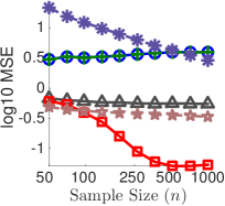
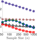
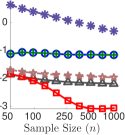
(a) $p(x)$	(b) $\mathbb{E}(x)$	(c) $\mathbb{E}(x^{2})$	(d) $\mathbb{E}(\cos(\omega x+b))$

Figure 6: Gaussian Mixture Example. (a) The contour of the distribution $p(x)$ that we use, and $\{x_{i}\}_{i=1}^{n}$ is generated by running $n$ independent MALA for $10$ steps. (b) - (c) The MSE of the different weighting schemes for estimating $\mathbb{E}(h(x))$, where $h(x)$ equals $x$, $x^{2}$, and $\cos(\omega x+b)$, respectively. For $h=\cos(\omega x+b)$ in (c), we draw $\omega\sim\mathcal{N}(0,1)$ and $b\sim\textrm{Uniform}([0,2\pi])$ and average the MSE over $20$ random trials.

References

Morris et al. (1996)
R. Morris, X. Descombes, and J. Zerubia.
The Ising/Potts model is not well suited to segmentation tasks.
In Digital Signal Processing Workshop Proceedings, 1996.,
IEEE, pages 263–266. IEEE, 1996.
Welling and Teh (2011)
M. Welling and Y. W. Teh.
Bayesian learning via stochastic gradient Langevin dynamics.
In ICML, 2011.
Alquier et al. (2016)
P. Alquier, N. Friel, R. Everitt, and A. Boland.
Noisy Monte Carlo: Convergence of markov chains with approximate
transition kernels.
Statistics and Computing, 26(1-2):29–47,
2016.
O’Hagan (1987)
A. O’Hagan.
Monte carlo is fundamentally unsound.
Journal of the Royal Statistical Society. Series D (The
Statistician), 36(2/3):247–249, 1987.
Henmi et al. (2007)
M. Henmi, R. Yoshida, and S. Eguchi.
Importance sampling via the estimated sampler.
Biometrika, 94(4):985–991, 2007.
Delyon and Portier (2014)
B. Delyon and F. Portier.
Integral approximation by kernel smoothing.
arXiv preprint arXiv:1409.0733, 2014.
Rezende and Mohamed (2015)
D. J. Rezende and S. Mohamed.
Variational inference with normalizing flows.
In ICML, 2015.
Efron (2012)
B. Efron.
Bayesian inference and the parametric bootstrap.
The annals of applied statistics, 6(4):1971, 2012.
Hazan et al. (2013)
T. Hazan, S. Maji, and T. Jaakkola.
On sampling from the gibbs distribution with random maximum
a-posteriori perturbations.
In NIPS, pages 1268–1276, 2013.
Papandreou and Yuille (2011)
G. Papandreou and A. L. Yuille.
Perturb-and-map random fields: Using discrete optimization to learn
and sample from energy models.
In ICCV, pages 193–200. IEEE, 2011.
Liu et al. (2015)
Q. Liu, J. W. Fisher III, and A. T. Ihler.
Probabilistic variational bounds for graphical models.
In NIPS, pages 1432–1440, 2015.
Wang et al. (2013)
C. Wang, X. Chen, A. J. Smola, and E. P. Xing.
Variance reduction for stochastic gradient optimization.
In Advances in Neural Information Processing Systems, pages
181–189, 2013.
Ranganath et al. (2014)
R. Ranganath, S. Gerrish, and D. M. Blei.
Black box variational inference.
In AISTATS, pages 814–822, 2014.
Greensmith et al. (2004)
E. Greensmith, P. L. Bartlett, and J. Baxter.
Variance reduction techniques for gradient estimates in reinforcement
learning.
Journal of Machine Learning Research, 5(Nov):1471–1530, 2004.
Sugiyama et al. (2008)
M. Sugiyama, S. Nakajima, H. Kashima, P. V. Buenau, and M. Kawanabe.
Direct importance estimation with model selection and its application
to covariate shift adaptation.
In NIPS, 2008.
Li et al. (2015)
L. Li, R. Munos, and C. Szepesvári.
Toward minimax off-policy value estimation.
In AISTATS, 2015.
Zhao and Zhang (2015)
P. Zhao and T. Zhang.
Stochastic optimization with importance sampling.
ICML, 2015.
Oates et al. (2017)
C. J. Oates, M. Girolami, and N. Chopin.
Control functionals for Monte Carlo integration.
Journal of the Royal Statistical Society, Series B, 2017.
Chwialkowski et al. (2016)
K. Chwialkowski, H. Strathmann, and A. Gretton.
A kernel test of goodness of fit.
In ICML, 2016.
Liu et al. (2016)
Q. Liu, J. D. Lee, and M. I. Jordan.
A kernelized stein discrepancy for goodness-of-fit tests and model
evaluation.
In ICML, 2016.
Briol et al. (2015a)
F.-X. Briol, C. Oates, M. Girolami, M. A. Osborne, D. Sejdinovic, et al.
Probabilistic integration: A role for statisticians in numerical
analysis?
arXiv preprint http://arxiv.org/abs/1512.00933,
2015a.
Briol et al. (2015b)
F.-X. Briol, C. Oates, M. Girolami, and M. A. Osborne.
Frank-Wolfe Bayesian Quadrature: Probabilistic integration with
theoretical guarantees.
In NIPS, 2015b.
O’Hagan (1991)
A. O’Hagan.
Bayes–Hermite quadrature.
Journal of statistical planning and inference, 29(3):245–260, 1991.
Ghahramani and Rasmussen (2002)
Z. Ghahramani and C. E. Rasmussen.