Quantum correlations and Bell’s inequality violation in a Heisenberg spin dimer via neutron scattering

Abstract

The characterization of quantum information quantifiers has attracted a considerable attention of the scientific community, since they are a useful tool to verify the presence of quantum correlations in a quantum system. In this context, in the present work we show a theoretical study of some quantifiers, such as entanglement witness, entanglement of formation, Bell’s inequality violation and geometric quantum discord as a function of the diffractive properties of neutron scattering. We provide one path toward identifying the presence of quantum correlations and quantum nonlocality in a molecular magnet as a Heisenberg spin-$1/2$ dimer, by diffractive properties typically obtained via neutron scattering experiments.

I Introduction

The study of quantum correlations has been subject of numerous investigations in the last few years, since it is a remarkable resource in quantum information science. In this regard, quantum information quantifiers Nielsen and Chuang (2010); Horodecki et al. (2009, 1996); Wieśniak et al. (2005); Souza et al. (2009); Wootters (1998); Hill and Wootters (1997); Brukner et al. (2006); Landau (1987); Souza et al. (2008); Ollivier and Zurek (2001); Vedral (2003); Liu et al. (2014); Ma et al. (2015); Girolami and Adesso (2011); Nakano et al. (2013); Cruz et al. (2016); Sarandy (2009); Paula et al. (2013); Montealegre et al. (2013); Luo (2008); Datta et al. (2008); Henderson and Vedral (2001); Paula et al. (2013); Montealegre et al. (2013); Huang (2013, 2014a) are useful tools to verify the presence of quantum correlations in a quantum system. In spite of that, the detection of quantum correlations is a difficult task, theoretically and experimentally speaking Cruz et al. (2016); Liu et al. (2014); Nakano et al. (2013); Girolami and Adesso (2011); Girolami et al. (2013, 2014); Luo (2008); Huang (2014b). Nowadays, it is understood that quantum correlations can be quantified through the measurements of some macroscopic properties of magnetic systems Cruz et al. (2016); Yurishchev (2011); Aldoshin et al. (2014); Liu et al. (2014).

The study of the magnetic properties of molecular materialsis typically done approximating magnetic parameters of a Hamiltonian model by the fit of some thermodynamic properties, such as magnetic susceptibility, internal energy and specific heat Reis (2013); Cruz et al. (2016); Haraldsen et al. (2005); Leite Ferreira et al. (2015); Esteves et al. (2014); Leite Ferreira et al. (2015). In this context, correlation functions have great importance in describing these properties; in addition, they can be directly measurable, e.g., in neutron scattering experiments via structure factors. Structure factors can be defined as two-point correlations Krammer et al. (2009) and are widely used to describe the crystal structure of molecular systems ruled by Hamiltonians Krammer et al. (2009); Tennant et al. (2003); Huberman et al. (2005), e.g., Heisenberg models Reis (2013).

Quantum information quantifiers are expressed in terms of statistical correlation functions Yurishchev (2011); Aldoshin et al. (2014); Cruz et al. (2016), due to the fact that these functions are present in the elements of the density matrix of the quantum system, linking their macroscopic properties with the quantum ones. Therefore, it is possible to quantify the presence of quantum correlations in a system via structure factors Cramer et al. (2011); Krammer et al. (2009); Liu et al. (2014); Marty et al. (2014), since these factors are directly associated to the correlation functions; thus allowing the measurement of quantum information quantifiers by neutron scattering experiments.

In this scenario, the present work shows analytical expressions for the entanglement witness, entanglement of formation, Bell’s inequality violation, and geometric quantum discord, based on the Schatten 1-norm as a function of quantities typically obtained in neutron scattering via a scalar structure factor. Our results provide one path toward identifying the presence of quantum correlations and quantum nonlocality in a molecular magnet such as a Heisenberg spin-$1/2$ dimer, by diffractive properties. This is an alternative way to describe the quantum properties of a sample material via neutron scattering experiments, without making any assumption about their macroscopic quantities, leading to promising applications in quantum information science.

II Neutron scattering for a Heisenberg spin dimer

The study of molecular magnetic materials is typically done through the approach of the magnetic parameters of a Hamiltonian model, by the fit of some thermodynamic properties, e.g., magnetic susceptibility, internal energy, and specific heat Reis (2013); Cruz et al. (2016); Haraldsen et al. (2005); Leite Ferreira et al. (2015); Esteves et al. (2014); Leite Ferreira et al. (2015). For a given Hamiltonian model, one can evaluate the inelastic structure factor, which allows a sensitive test of the assumed model, since their properties are affected by the relative positions of the metallic centers of a sample material Haraldsen et al. (2005).

Let us consider a molecular magnet as an interacting pair of spin-$1/2$ ruled by the Heisenberg-Dirac-Van Vleck Hamiltonian,

$$\mathcal{H} = -J\vec{S}_{1}\cdot\vec{S}_{2}\leavevmode\nobreak\ .$$ (1)

This is an ideal realization of a two qubit system; and therefore, a promising platform in the quantum information processing.

Once Eq. (1) is invariant under spin rotation, the total spin $s=s_{1}+s_{2}$ is a good quantum number Haraldsen et al. (2005); Reis (2013). From the Clebsch-Gordon series the spectrum consists in an $s=1$ triplet and $s=0$ singlet Reis (2013). Diagonalizing it, we obtain the energy eigenvalues $E_{s}$ and eigenvectors $|s,m_{s}\rangle$ Haraldsen et al. (2005); Reis (2013):

$$E_{s=1}=\frac{1}{4}J$$ (2)

$$E_{s=0}=-\frac{3}{4}J$$ (3)

$$|s=1,m_{s}=+1\rangle=|00\rangle$$ (4)

$$|s=1,m_{s}=0\rangle=\frac{1}{\sqrt{2}}\left(|01\rangle+|10\rangle\right)$$ (5)

$$|s=1,m_{s}=-1\rangle=|11\rangle$$ (6)

$$|s=0,m_{s}=0\rangle=\frac{1}{\sqrt{2}}\left(|01\rangle{-}|10\rangle\right)\leavevmode\nobreak\ .$$ (7)

In magnetic neutron scattering, neutrons interact magnetically with the atoms of the target sample. From the Van Hove formalism Van Hove (1954), the partial differential cross section of an incident neutron in a magnetic system with initial state $|\psi_{i}\rangle$ is expressed in terms of time-dependent correlation functions

$$\frac{d^{2}\sigma}{d\omega d\Omega} = \frac{1}{Z}\left(\frac{g_{i,\alpha}\gamma r_{0}}{2}\right)^{2}$$ (8)

$$\times\sum_{\alpha,\beta,l,m}\left(\delta_{\alpha,\beta}-\frac{\vec{q_{\alpha}}\vec{q_{\beta}}}{|\vec{q}|^{2}}\right)\left[F_{l}(\vec{q})g_{l,\alpha}\right]^{*}\left[F_{m}(\vec{q})g_{m,\beta}\right]$$

$$\times\int\frac{dt}{2\pi}e^{i\left[\omega t+\vec{q}\cdot\left(\vec{r_{l}}-\vec{r_{m}}\right)\right]}\langle\psi_{i}|S_{l}^{\alpha}S_{m}^{\beta}(t)|\psi_{i}\rangle,$$

where the sum run over all magnetic sites $l$ and $m$, which are the l-th and m-th spins with position vectors $\vec{r_{l}}$ and $\vec{r_{m}}$, respectively. Furthermore, $\gamma$ is the neutron magnetic moment; $r_{0}=e^{2}/m_{e}c^{2}$ is the classical electron radius; $F_{i}(\vec{q})$ is the magnetic form factor; $\alpha$,$\beta=x,y,z$; $\omega$ is the energy transferred to the target magnetic system; $\vec{q}=\vec{k}_{out}-\vec{k}_{in}$ is the difference between the final and the initial wave vectors (scattering vector); and finally, $S_{l}^{\alpha}$ are the spin operators. Thus, the differential cross section is proportional to the neutron scattering structure factor tensor that is written in terms of the pairwise correlation functionMarty et al. (2014); Zaliznyak and Lee (2005); Liu et al. (2014); Cramer et al. (2011):

$$\mathcal{S}^{(\alpha,\beta)}(\vec{q},\omega)=\int\frac{dt}{2\pi}\sum_{l,m}e^{i\left[\omega t+\vec{q}\cdot\left(\vec{r_{l}}-\vec{r_{m}}\right)\right]}\langle\psi_{i}|S_{l}^{\alpha}S_{m}^{\beta}(t)|\psi_{i}\rangle.$$

(9)

Due to the transitions between the discrete energy levels, Eq. (2)-(3), the time integral shown in Eq. (9) gives a delta function $\delta\left(E_{f}-E_{i}-\hbar\omega\right)$, where $\hbar\omega$ is the transfer energy Haraldsen et al. (2005). Integrating Eq.(9) over energies, we obtain the integrated structure factor Krammer et al. (2009); Marty et al. (2014); Cramer et al. (2011)

$$\bar{\mathcal{S}}(\vec{q})=\sum_{\alpha,\beta}{\mathcal{S}}^{\alpha\beta}(\vec{q})=\sum_{\alpha,\beta}\sum_{l,m}e^{i\vec{q}\cdot\left(\vec{r_{l}}-\vec{r_{m}}\right)}\langle S_{l}^{\alpha}S_{m}^{\beta}\rangle.$$ (10)

Therefore, for the specific case of a Heisenberg spin dimer, Eq.(1), one can define the so-called exclusive structure factor as a function of the scattering vector $\vec{q}$ Haraldsen et al. (2005), for the excitation of the final states in the magnetic multiplet $|\psi_{f}\rangle$, Eq.(4)-(7), from the given initial state $|\psi_{i}\rangle$

$$\mathcal{S}^{(\alpha,\beta)}_{fi}(\vec{q})=\sum_{f}\langle\psi_{i}|\mathcal{U}_{\alpha}^{\dagger}(\vec{q})|\psi_{f}\rangle\langle\psi_{f}|\mathcal{U}_{\beta}(\vec{q})|\psi_{i}\rangle,$$ (11)

where

$$\mathcal{U}_{\alpha,\beta}(\vec{q})=\sum_{\vec{r}_{l}}S_{l}^{(\alpha,\beta)}e^{i\vec{q}\cdot r_{l}},$$ (12)

and the sum taken over all magnetic ions in a unit cell Haraldsen et al. (2005); Liu et al. (2014); Marty et al. (2014).

For the $|s=0,m_{s}=0\rangle$ initial state (antiparallel magnetic alignment), Eq.(7), only $s=1$ final states are excited, Eq.(4)-(6). Thus, one can define the scalar neutron scattering structure factor, $\mathcal{S}(\vec{q})$, for the Heisenberg $1/2$-spin dimer Haraldsen et al. (2005) by

$$\mathcal{S}^{(\alpha,\beta)}_{fi}(\vec{q})=\delta_{\alpha,\beta}\mathcal{S}(\vec{q}).$$ (13)

Using the eigenvectors given by Eq.(4)-(7) in Eq.(11), we evaluate the inelastic neutron scattering intensities, that are given by structure factors Haraldsen et al. (2005) for the Heisenberg spin-$1/2$ dimer, Eq. (1). Thus, we obtain the scalar neutron scattering structure factor as calculated in reference Haraldsen et al., 2005:

$$\mathcal{S}(\vec{q})=\frac{1}{2}\left[1-cos(\vec{q}\cdot\left(\vec{r_{1}}-\vec{r_{2}}\right))\right].$$ (14)

Thus, given the Hamiltonian model, it is possible to predict their scalar structure factor, which can be compared to the neutron scattering experiments results Haraldsen et al. (2005).

III Quantum information-theoretic quantifiers in a Heisenberg spin dimer

In this section, we will present the analytical expressions for quantum information quantifiers, such as entanglement witness, entanglement of formation, Bell’s inequality violation and geometric quantum discord, based on the Schatten 1-norm as a function of quantities typically obtained in neutron scattering via scalar structure factor, allowing their measurement via neutron scattering experiments.

III.1 Spin-Spin Correlation Function

Correlation functions have a great importance in statistical physics and quantum mechanics, allowing us to find different properties of a physical system. In addition, it can be directly measurable, e.g., in scattering experiments Aldoshin et al. (2014). Quantum information quantifiers are expressed in terms of statistical correlation functions Yurishchev (2011); Aldoshin et al. (2014); Cruz et al. (2016), due to the fact that these functions are present in the elements of the density matrix of the quantum system, linking their macroscopic and structural properties with the quantum ones.

For the system ruled by the Hamiltonian, Eq.(1), from the Eq.(10) and Eq.(13) the spin-spin correlation function can be extracted and written in terms of integrated structure factor

$$\mathcal{C} = \langle S_{1}^{\alpha}S_{2}^{\alpha}\rangle=e^{-i\vec{q}\cdot\left(\vec{r_{1}}-\vec{r_{2}}\right)}\mathcal{S}^{\alpha\alpha}(\vec{q}),$$ (15)

where $\alpha=x,y,z$.

Thus, spin-spin correlation function can be accessed through diffractive properties obtained via neutron scattering experiments, without making any assumption about the macroscopic properties of the measured system or the external conditions under which the neutrons are scattered.

Using Eq.(14) spin-spin correlation function can be written as a function of the the scattering vector, $\vec{q}=\vec{k}_{out}-\vec{k}_{in}$, i.e., the difference between the final and the initial wave vectors, and the the difference between the position vectors $\vec{r_{1}}$ and $\vec{r_{2}}$ of the metallic centers.

$$\mathcal{C} = \frac{e^{-i\vec{q}\left(\vec{r_{1}}-\vec{r_{2}}\right)}}{2}\left[1-cos(\vec{q}\cdot\left(\vec{r_{1}}-\vec{r_{2}}\right))\right]\leavevmode\nobreak\ ,$$ (16)

this last ranges from $-1\leq\mathcal{C}\leq 0$ for antiparallel magnetic alignment ($J<0$ - entangled ground state) and $0<\mathcal{C}\leq 1/3$ for parallel magnetic alignment ($J>0$ - separable ground state) Cruz et al. (2016); Yurishchev (2011); Aldoshin et al. (2014).

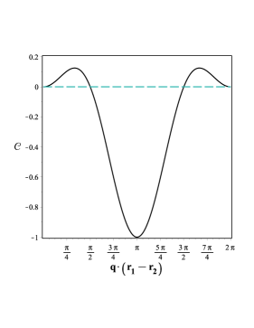
Figure 1: Spin-spin correlation as a function of $\vec{q}\cdot\left(\vec{r_{1}}-\vec{r_{2}}\right)$, Eq.(16). The dashed (green) horizontal line separates the regions with antiparallel magnetic alignment ($\pi/2\leq\vec{q}\cdot\left(r_{1}-r_{2}\right)\leq 3\pi/2$) and parallel magnetic alignment ($0<\vec{q}\cdot\left(r_{1}-r_{2}\right)<\pi/2$ and $3\pi/2<\vec{q}\cdot\left(r_{1}-r_{2}\right)<2\pi$ ).

The spin-spin correlation function, Eq. (16), is depicted in Fig. (1) as a function of the scattering vector $\vec{q}$ times the distance between the metallic centers of a sample material $\vec{r_{1}}-\vec{r_{2}}$, which can be obtained by neutron scattering experiments. It is worth noting that, the location of the zero point correlation can provide a convenient estimate for which distances in the system can be found in an antiparallel magnetic alignment ($\pi q^{-1}/2\leq r_{1}-r_{2}\leq 3\pi q^{-1}/2$) or a parallel magnetic alignment ($0<r_{1}-r_{2}<\pi q^{-1}/2$ and $3\pi q^{-1}/2<r_{1}-r_{2}<2\pi q^{-1}$ ), without any assumption about macroscopic quantities, such as the temperature, magnetic field, magnetic susceptibility, internal energy or specific heat. This result has a great importance to guide us through the study of the quantum information quantifiers in a Heisenberg spin dimer, since these quantifiers depend directly on the spin-spin correlation function.

III.2 Entanglement Witness

The detection of entanglement is usually done using an observable which identifies the presence of entanglement in a quantum system Horodecki et al. (2009, 1996); Wieśniak et al. (2005); Souza et al. (2009). This observable, the so-called entanglement witness ($\mathcal{W}$), has a negative expectation value whether the system is in an entangled quantum state ($\mathcal{W}<0$) and otherwise positive. However, the positive expectation value does not imply the presence of separable quantum states. Recently magnetic susceptibility was proposed as a thermodynamical entanglement witness Horodecki et al. (2009, 1996); Wieśniak et al. (2005); Souza et al. (2009). For a system in which $[\mathcal{H},S_{z}]$ the average magnetic susceptibility in a complete separable state satisfies Wieśniak et al. (2005); Souza et al. (2009)

$$\bar{\chi}=\frac{\chi_{x}+\chi_{y}+\chi_{z}}{3}\leqslant\frac{(g\mu_{B})^{2}NS}{3k_{B}T},$$ (17)

where $N$ is the number of magnetic ions with spins-$S$, $k_{B}$ is the Boltzmann constant, $\mu_{B}$ is the Bohr magneton, $g$ is the Landé factor and $\bar{\chi}$ is the average of the magnetic susceptibility.

As calculated by Wieśniak, Vedral and Brukner in the reference Wieśniak et al., 2005, the entanglement witness can be calculated in terms of the average magnetic susceptibility:

$$\mathbb{W}=\frac{3k_{B}T\bar{\chi}}{(g\mu_{B})^{2}NS}-1.$$ (18)

In reference Brukner et al., 2006, the magnetic susceptibility of an antiferromagnetic spin-1/2 chain is compared to the correlation function measured by neutron diffraction Soares-Pinto et al. (2009). The pairwise average magnetic susceptibility must be written as a function of the pairwise correlation, Eq.(16), as

$$\bar{\chi}(T)=\frac{N(g\mu_{B})^{2}(1+\mathcal{C})}{2k_{B}T}.$$ (19)

Thus, we can analytically calculate the entanglement witness for a molecular magnet, Eq.(18), such as a Heisenberg spin-$1/2$ dimer, in terms of their scalar structure factor using Eq.(16), (18) and (19)

$$\mathbb{W} = 2+3e^{-i\vec{q}\left(\vec{r_{1}}-\vec{r_{2}}\right)}\mathcal{S}(\vec{q})$$ (20)

$$= 2+\frac{3e^{-i\vec{q}\left(\vec{r_{1}}-\vec{r_{2}}\right)}}{2}\left[1-cos(\vec{q}\cdot\left(\vec{r_{1}}-\vec{r_{2}}\right))\right].$$

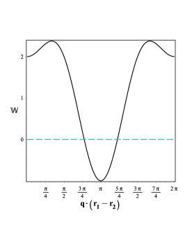
Figure 2: Entanglement witness of a Heisenberg spin dimer, Eq.(20). The dashed (green) horizontal line separates the region where the witness has a negative expectation value, i.e., the system is in an entangled quantum state $2.45<\vec{q}\cdot\left(\vec{r_{1}}-\vec{r_{2}}\right)<3.85$.

In Fig. 2, we show the entanglement witness for a Heisenberg spin dimer, Eq. (20), as a function of $\vec{q}\cdot\left(r_{1}-r_{2}\right)$. The witness has a negative expectation at the range $2.45<\vec{q}\cdot\left(\vec{r_{1}}-\vec{r_{2}}\right)<3.85$, revealing the presence of entangled states. This result is compatible to the last ones, since in this band the system is found in an antiparallel magnetic alignment (entangled ground state), as can be seen in Fig. 1. Thus, we provide one way to identify the presence of entanglement in a molecular magnet, such as a Heisenberg spin dimer, by diffractive properties obtained via neutron scattering experiments, without making any assumption about their macroscopic quantities.

III.3 Entanglement of Formation

In order to quantify the amount of entanglement in the Heisenberg spin-$1/2$ dimer and make a comparison with the entanglement witness, we will adopt the measurement of entanglement of formation defined by Wootters (1998); Hill and Wootters (1997):

$$\mathbb{E}=-\Gamma_{+}\log_{2}\left(\Gamma_{+}\right)-\Gamma_{-}\log_{2}\left(\Gamma_{-}\right),$$ (21)

with

$$\Gamma_{\pm}=\frac{1\pm\sqrt{1-\mathbb{C}^{2}}}{2},$$ (22)

where $\mathbb{C}$ is the concurrence Wootters (1998); Hill and Wootters (1997); Nielsen and Chuang (2010); Horodecki et al. (2009). The concurrence can be written as a function of the scalar structure factor, Eq.(14), in terms of spin-spin correlation function, Eq.(16), as follows:

$$\mathbb{C}=\mbox{max}\left[0,-\frac{1}{2}\left(1+3e^{-i\vec{q}\left(\vec{r_{1}}-\vec{r_{2}}\right)}\mathcal{S}(\vec{q})\right)\right].$$ (23)

The equation above shows that the concurrence of a Heisenberg spin-$1/2$ dimer is also related to the diffractive properties, which can be obtained by neutron scattering experiments.

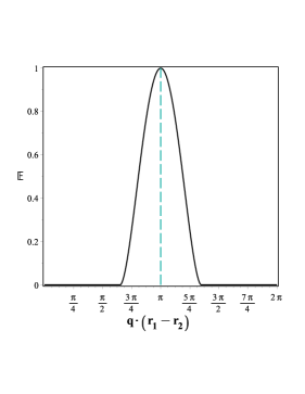
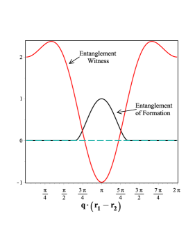
Figure 3: (a) Entanglement of formation as a function of $\vec{q}\cdot\left(\vec{r_{1}}-\vec{r_{2}}\right)$, Eq.(21). The dashed (green) vertical line highlights the maximum of entanglement, where the system is in an antiparallel magnetic alignment with an entangled pure state. (b) We make a comparison between the entanglement of formation and the entanglement witness. The dashed (green) horizontal line separates the region where the witness has a negative expectation value, i.e., the system is in an entangled quantum state.

In sequence, we shown in Fig. 3 (a) the entanglement of formation as a function of the scattering vector $\vec{q}$ times the distance between the metallic centers $\vec{r_{1}}-\vec{r_{2}}$ of a Heisenberg spin dimer, Eq.(21). It is possible to identify a maximum of entanglement at $r_{1}-r_{2}=\pi q^{-1}$, where the system is found in an antiparallel magnetic alignment with an entangled pure state. It is worth noting that there are entangled states at $2.0\lesssim\vec{q}\cdot\left(r_{1}-r_{2}\right)\lesssim 4.2$, above the band where the entanglement is identified on the entanglement witness. In Fig. 3 (b), we make a comparison between the entanglement of formation and the entanglement witness. As can be seen, the positive expectation value of the witness, separated by the dashed (green) line, does not imply separability. However, the negative expectation value necessarily implies in the presence of entangled quantum states in the system.

III.4 Bell’s Inequality Violation

Bell’s inequality violation Landau (1987) has an important role in the quantum information theory, as a necessary and sufficient condition for the usefulness of quantum states in the communication complexity of protocols Brukner et al. (2004). For a Heisenberg spin-$1/2$ dimer, the Bell’s inequality test Souza et al. (2009, 2008) is related to the measurement of the Bell operator Souza et al. (2009)

$$\mathbb{B}=\vec{n_{1}}\cdot\vec{S}\otimes\left(\vec{n_{2}}\cdot\vec{S}-\vec{n_{4}}\cdot\vec{S}\right)+\vec{n_{3}}\cdot\vec{S}\otimes\left(\vec{n_{2}}\cdot\vec{S}+\vec{n_{4}}\cdot\vec{S}\right),$$ (24)

where $\vec{n_{1}}\cdot\vec{S}$ is the projection of the spin on the direction $n$.

Using the set of directions $\{\vec{n_{1}},\vec{n_{2}},\vec{n_{3}},\vec{n_{4}}\}=\{(0,0,1),(-1,0,-1)/\sqrt{2},(-1,0,0),(-1,0,1)/\sqrt{2}\}$, the Eq. (24) becomes $\mathbb{B}=\sqrt{2}\left(S_{x}\otimes S_{x}+S_{z}\otimes S_{z}\right)$. Therefore

$$|\langle\mathbb{B}\rangle| = 2\sqrt{2}|\mathcal{S}(\vec{q})|$$ (25)

$$= 2\sqrt{2}\left|1-cos(\vec{q}\cdot\left(\vec{r_{1}}-\vec{r_{2}}\right))\right|.$$

Thus, from Eq.(25), it is possible to verify whether there is a Bell’s inequality violation via neutron scattering experiments.

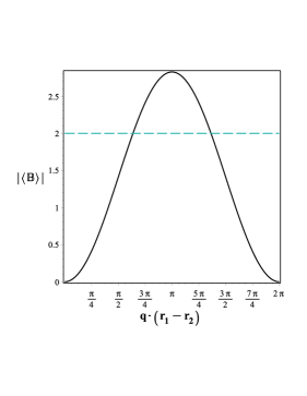
Figure 4: Mean value of Bell operator as a function of $\vec{q}\cdot\left(\vec{r_{1}}-\vec{r_{2}}\right)$, Eq.(25). The dashed (green) horizontal line separates the region where the Heisenberg dimer violates the Bell’s inequality.

In Fig. 4, we shown the mean value of the Bell operator as a function of the scattering vector $\vec{q}$ times the distance between the metallic centers $\vec{r_{1}}-\vec{r_{2}}$ of a target sample of neutron scattering, Eq.(25). As can be seen, the Bell’s inequality is violated in $2.0\lesssim\vec{q}\cdot\left(r_{1}-r_{2}\right)\lesssim 4.2$, where there is a maximum violation in $r_{1}-r_{2}=\pi q^{-1}$, when the system is in an entangled pure state, see Fig. 3 (a). It is compatible to the previous result obtained from the entanglement of formation, where we found entangled quantum states at the same band. Therefore, it is possible to verify the quantum nonlocality in a Heisenberg spin dimer by diffractive properties obtained in neutron scattering experiments.

III.5 Geometric Quantum Discord

Despite quantum entanglement providing one path toward finding pure quantum correlations, it does not encompass all quantum correlations in a system. The measurement of the total amount of quantum correlations has been called quantum discord Ollivier and Zurek (2001); Vedral (2003); Liu et al. (2014); Ma et al. (2015); Girolami and Adesso (2011); Nakano et al. (2013); Cruz et al. (2016); Sarandy (2009); Paula et al. (2013); Montealegre et al. (2013); Luo (2008); Datta et al. (2008); Henderson and Vedral (2001).

The calculation of quantum discord is a rather complicated task, even for a two-qubit system, such as a Heisenberg spin-$1/2$ dimer Cruz et al. (2016); Paula et al. (2013). This fact has stimulated alternative measurements of quantum information-theoretical quantifiers as the geometric quantum discord Cruz et al. (2016). In this context, the geometric quantum discord, based on the Schatten 1-norm, is one path toward achieving a well-defined measurement of quantum correlations in a quantum system Cruz et al. (2016) and it can be defined as

$$\mathbb{Q}_{G}(\rho)=\min_{\omega}\|\rho-\rho_{c}\|,$$ (26)

where $\|X\|=\mbox{Tr}\left[\sqrt{X^{\dagger}X}\right]$ is the 1-norm, $\rho$ is a given quantum state and $\omega$ is the set of closest classical-quantum states $\rho_{c}$ Paula et al. (2013); Montealegre et al. (2013); Cruz et al. (2016), whose general form is given by:

$$\rho_{c}=\sum_{k}p_{k}\Pi_{k}^{\{1\}}\otimes\rho_{k}^{\{2\}},$$ (27)

with $0\leq{p_{k}}\leq 1$ and $\sum_{k}p_{k}=1$; $\{\Pi_{k}^{\{1\}}\}$ denotes a set of orthogonal projectors for subsystem $1$, and $\rho_{k}^{\{2\}}$ is a general reduced density operator for the subsystem $2$ Paula et al. (2013); Montealegre et al. (2013).

Thus, for a Heisenberg spin dimer, the geometric quantum discord, based on the Schatten 1-norm, is written as a function of the scalar structure factor as:

$$\mathbb{Q}_{G}(\mathcal{S}) = \left|\frac{1}{4}\mathcal{S}(\vec{q})\right|$$ (28)

$$= \left|\frac{1-cos(\vec{q}\cdot\left(\vec{r_{1}}-\vec{r_{2}}\right))}{4}\right|\leavevmode\nobreak\ .$$

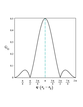
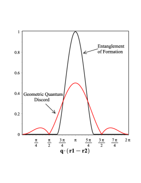
Figure 5: (a) Geometric quantum discord as a function of $\vec{q}\cdot\left(\vec{r_{1}}-\vec{r_{2}}\right)$. Dashed (green) vertical line highlights the point where the system is in an antiparallel magnetic alignment with an entangled pure state. (b) We make a comparison between the geometric quantum discord and the entanglement of formation; it is possible to identify the presence of quantum correlations when the entanglement is absent and even when the system is found in a parallel magnetic alignment with a separable quantum state.

Fig. 5 (a) shows the geometric quantum discord as a function of the scattering vector $\vec{q}$ times the distance between the metallic centers $\vec{r_{1}}-\vec{r_{2}}$ of a sample material, Eq.(28). We identify a maximum of quantum correlation at $r_{1}-r_{2}=\pi q^{-1}$, this is compatible to the previous results, where at this point the system is found in an entangled pure state, see Fig. 3 (a). Fig. 5 (b) makes a comparison between the geometric quantum discord and the entanglement of formation. As can be seen, it is possible to identify the presence of quantum correlations when the entanglement is absent and even when the system is found in a parallel magnetic alignment with a separable quantum state ($0<\vec{q}\cdot\left(r_{1}-r_{2}\right)<\pi/2$ and $3\pi/2<\vec{q}\cdot\left(r_{1}-r_{2}\right)<2\pi$ ), see Fig. 1; furthermore, the points of zero discord coincide with the points of zero correlation ($\pi/2$ and $3\pi/2$), indicating the absence of magnetic interaction ($J=0$) between the magnetic ions.

Therefore, we provide one way to find the geometric quantum correlations in a Heisenberg spin dimer, by diffractive properties obtained via neutron scattering experiments, without making any assumption about their macroscopic quantities.

IV Conclusions

In summary, our main result was to provide to the literature analytical expressions for quantum information quantifiers, such as the entanglement witness, entanglement of formation, Bell’s inequality violation and geometric quantum discord as a function of quantities typically obtained in neutron scattering via scalar structure factor. We provide one path toward identifying the presence of quantum correlations and quantum nonlocality in a two-qubit system such as a Heisenberg spin-$1/2$ dimer, using diffractive properties without making any assumptions about their macroscopic quantities. We present an alternative way to describe the quantum properties of a sample material via neutron scattering experiments. Our results open doors for the detection and manipulation of quantum correlations through neutron scattering experiments in magnetic systems, such as the molecular magnets ruled by Heisenberg Hamiltonians; leading to promising applications in quantum information science, since these materials can be promising platforms in quantum information processing.