Mitigating the Influence of the Boundary on PDE-based Covariance Operators

Abstract.

Gaussian random fields over infinite-dimensional Hilbert spaces require the definition of appropriate covariance operators. The use of elliptic PDE operators to construct covariance operators allows to build on fast PDE solvers for manipulations with the resulting covariance and precision operators. However, PDE operators require a choice of boundary conditions, and this choice can have a strong and usually undesired influence on the Gaussian random field. We propose two techniques that allow to ameliorate these boundary effects for large-scale problems. The first approach combines the elliptic PDE operator with a Robin boundary condition, where a varying Robin coefficient is computed from an optimization problem. The second approach normalizes the pointwise variance by rescaling the covariance operator. These approaches can be used individually or can be combined. We study properties of these approaches, and discuss their computational complexity. The performance of our approaches is studied for random fields defined over simple and complex two- and three-dimensional domains.

Courant Institute, New York University

New York, NY 10012, USA

1. Introduction

Gaussian random fields over functions, sometimes referred to as continuously indexed Gaussian random fields, are important in spatial statistical modeling, geostatistics and in inverse problems. They are described through a mean and a covariance operator, usually defined over a Hilbert space. Efficient manipulation of random fields is of critical importance in applications. In particular, one commonly requires the application of the covariance operator and of its inverse, the precision operator, to vectors from the function space. Additionally, computation of realizations from the distribution requires the ability to apply a square root of the covariance operator to vectors.

Constructing covariance operators from elliptic PDE operators, which has recently gained popularity [1, 2, 3, 4, 5], allows one to build on available fast PDE solvers for the required manipulations. This leads to a correspondence between domain Green’s functions of PDE operators and covariance functions of the Gaussian random fields. On bounded domains, PDE operators require the definition of boundary conditions, which has implications for the resulting covariance operators. Namely, this can lead to increased/decreased correlation and pointwise variance close to the boundary, which is usually undesirable from a statistical perspective. This behavior is illustrated in figure 1 and has also been observed in [2, 3, 4]. In this work, we present methods to ameliorate these boundary effects. Since we aim at large-scale problems, we are interested in scalable optimal complexity algorithms that avoid dense matrix operations or matrix assembly. Our target is to find domain Green’s functions that are as similar as possible to the free-space Green’s functions of the precision operator, which are Matérn covariance functions. We present two methods towards achieving this objective.

The first method combines the PDE operator with a homogeneous Robin boundary condition $\beta u+\frac{\partial u}{dn}=0$, with a varying Robin coefficient $\beta=\beta({\boldsymbol{x}})$. This coefficient function is derived as solution to an optimization problem that aims at making the difference between the domain and the free-space Green’s functions small. Our approach exploits the definition of the domain Green’s function and uses the fact that explicit expressions for the free-space Green’s functions are available or can easily be computed numerically. For one-dimensional domains, $\beta$ can be chosen such that the effect of boundary conditions vanishes completely. For two- and three-dimensional domains, $\beta$ can be chosen to minimize boundary effects in an averaged sense. The approach only requires computation of inner products and is thus feasible for large-scale problems.

The second method we propose amounts to a rescaling of the covariance operator $\mathcal{C}$ that is constructed from elliptic PDE operators. It can be combined with the approach discussed above. This rescaled operator has constant pointwise variance (a property that $\mathcal{C}$ above does not have). The idea is most easily understood in finite dimensions: For a covariance matrix $\Sigma$, with diagonal $D_{ij}:=\Sigma_{ij}\delta_{ij}$, the rescaled matrix $\Sigma^{\prime}=D^{-\frac{1}{2}}\Sigma D^{-\frac{1}{2}}$ is also a covariance matrix, and it has a constant unit diagonal.

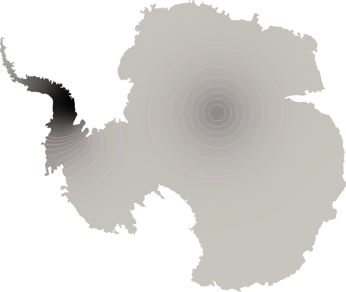
Figure 1. Left: Cross sections through covariance functions induced by elliptic PDE operators with different boundary conditions. Shown is also a sketch of the domain $\Omega=[0,1]^{2}$ and the cross section ${\boldsymbol{x}}(s)=(s,0.5)^{T}$. The center is located at ${\boldsymbol{x}}^{\star}={\boldsymbol{x}}(0.05)=(0.05,0.5)^{T}$. Right: Two covariance functions on the Antarctica domain (see Sec. 6.2). The magnitude of the left covariance function exceeds the gray scale used to show the covariance between the centers and the points of the domain. The discrepancy between the covariance is due to the use of Neumann boundary conditions for the differential operator.

Related Work

In spatial statistics, the use of covariance operators is motivated by the need for fast computations [6, 7]. The connection between inverse elliptic operators and Gaussian fields was originally established in [8]. Building on this connection and results in [9], the authors of [3] show that discretizing an inverse elliptic covariance operator is valid, from a statistical perspective. This results in a (discretely-indexed) Gaussian field with a sparse precision operator due to the locality of differential operators. This sparsity allows for fast application of the precision. Fast application of the covariance operator is possible building on fast elliptic PDE solvers.

A parallel approach aiming at Bayesian inverse problems was established by Stuart [1]. Contrary to [3], the author’s motivation is to develop the theory of Bayesian inference in function spaces. The advocated approach (which we follow) is that all algorithms should be presented and studied in function spaces, i.e., in infinite dimensions. Taking this approach, the author is lead to the use of “Laplacian-like” precision operators [1, Assumption 2.9], which are used to define Gaussian priors for Bayesian inverse problems. In some respect, [1] and [3, 6] draw similar conclusions. They argue that using covariance operators is superior to using covariance functions, both from a theoretical as well as from a computational perspective.

The role of PDE-operator boundary conditions if the domain $\Omega\subseteq\mathbb{R}^{d}$ is bounded was already observed to cause variance inflation near the boundary in [3]. To avoid this effect, domain extension was proposed in [3, 6, 4]. As an alternative and related to one of the methods we propose in this paper, in [4] the authors propose to use a Robin boundary condition of the form $\beta u+\frac{\partial u}{\partial n}=0$. They conduct numerical experiments to empirically find a constant, boundary effect mitigating coefficient $\beta$ in the Robin condition for a two-dimensional circular domain. In [10] the authors suggest sampling values on the boundary according to the correct distribution and then using these values as Dirichlet data for the domain. This approach is technical in higher dimensions and it requires assembled matrices.

Contributions

The main contributions of this work are as follows: (1) The proposed methods mitigate boundary effects arising in continuously indexed Gaussian random fields when elliptic PDE operators are used to construct covariance operators. They are computationally feasible, do not require assembled matrices, nor the extension of the computational domain. (2) We present simple and fast algorithms for the approximation of the quantities used in our methods. Once these upfront computations, which depend on the domain and the PDE operator, are available, all remaining computations (covariance and precision application, and computation of samples) are as efficient as in the original method. (3) We perform a comprehensive numerical study of the proposed methods on simple as well as complex geometries, such as the Antarctica domain from [5].

Limitations

We also remark limitations of our methods. (1) To compute the optimal Robin coefficient, an integration over the domain must be performed for each point on the boundary, where the Robin coefficient is needed. However, this integration can be accelerated by realizing that in many cases the Robin coefficient varies smoothly, and hence one may use interpolation between adjacent points. Moreover, the integrands decay rapidly and thus the integration can be restricted to a small part of the domain. (2) Computation of the integrals in the Robin method can be challenging due to the singularity of the integrands. As a remedy, we discuss approximations that allow computation of these integrals at an accuracy that suffices for our purposes. (3) For the variance normalization method, we require knowledge of the pointwise variance over the domain. Fortunately, this field is often smooth and thus interpolation from a few points to the entire domain is possible. Additionally, one can leverage potential symmetries in the geometry to speed up the computation of the pointwise variance. (4) The upfront computations our methods require depend on the PDE operator used to define the covariance operator. If one uses a hierarchical method in which the PDE operator varies, the proposed approach can become computationally expensive.

2. Preliminaries

Let $\Omega\subseteq\mathbb{R}^{d}$, $d=1,2,3$ be a bounded open domain with piecewise smooth boundary $\partial\Omega$. Throughout this paper, we are concerned with Gaussian measures over spaces of functions defined on $\Omega$. We first recall definitions of Gaussian measures and Gaussian fields—see, e.g., [11, 12] for details.

2.1. Gaussian measures

Let $\mu$ a measure on a separable Banach space $X$ and $u\sim\mu$. We say $\mu$ is Gaussian if $\forall\ell\in X^{*}$, if there exist $m_{\ell}$ real and $\sigma_{\ell}$ non-negative such that $\ell(u)\sim\mathcal{N}(m_{\ell},\sigma_{\ell})$ is Gaussian. Consider $X=C(\Omega)$, the space of continuous functions on $\Omega$ with the $\sup$-norm, so that $X\subseteq L^{2}(\Omega)$. Taking this view, one can specify a Gaussian measure $\mu$ on $X$ by first taking a mean $m\in X$ and a (linear) self-adjoint positive definite trace class covariance operator $\mathcal{C}:L^{2}(\Omega)\to L^{2}(\Omega)$. Since samples $\mathcal{N}(m,\mathcal{C})$ are continuous for the choices of $\mathcal{C}$ we consider below, $X$ has full measure and by [11, Ex. 3.39] we have a Gaussian measure on $C(\Omega)$. We still write $\mathcal{N}(m,\mathcal{C})$ for the corresponding Gaussian measure on $X$. If $h\in L^{2}(\Omega)$ is discontinuous, then $\mathcal{C}^{-1}h$ is empty and $\langle h,\mathcal{C}^{-1}h\rangle=\|\mathcal{C}^{-\frac{1}{2}}h\|=\infty$, informally making the likelihood of observing $h$ zero. Thus, the Gaussian measure gives full measure to $X$.

2.2. Gaussian random fields

For our purposes, a Gaussian random field is a random function $u:\Omega\to\mathbb{R}$ such that for all finite sets $\{{\boldsymbol{x}}_{i}\}_{i=1}^{n}\subseteq\Omega$, the random vector $(u({\boldsymbol{x}}_{1}),...,u({\boldsymbol{x}}_{n}))^{T}$ is a multivariate normal. For simplicity, here we consider a centered field, i.e., $m({\boldsymbol{x}}):=\mathbb{E}[u({\boldsymbol{x}})]\equiv 0$. The corresponding covariance function $c:\Omega\times\Omega\to\mathbb{R}$ is defined as $c({\boldsymbol{x}},{\boldsymbol{y}}):=\mathbb{E}[u({\boldsymbol{x}})u({\boldsymbol{y}})]$. A covariance function can also be used as a kernel for an integral operator. The resulting operator is given by

$$(\mathcal{C}f)({\boldsymbol{x}})=\int_{\Omega}c({\boldsymbol{x}},{\boldsymbol{y}})f({\boldsymbol{y}})d{\boldsymbol{y}}.$$

If $c$ is positive-definite [Varadhan01], $\mathcal{C}$ is a valid covariance operator in the sense of section 2.1. This connection motivates considering $\mathcal{C}$ to be an inverse elliptic operator, making $c$ the Green’s function of that operator. In this case, writing $c({\boldsymbol{x}},{\boldsymbol{y}})=(\mathcal{C}\delta_{{\boldsymbol{x}}})({\boldsymbol{y}})$ is well-defined from a PDE perspective and we use this identity below. Now, the connection with Gaussian measures is straightforward—a Gaussian random field defines a Gaussian measure on $C(\Omega)$.

2.3. Inverse elliptic covariance operators

On $\Omega$, consider the elliptic differential operator

$$\mathcal{A}:=-\gamma\Delta+\alpha$$ (1)

with constants $\gamma,\alpha>0$. The domain on which $\mathcal{A}$ is defined depends on the choice of boundary conditions. We will discuss different domains $\mathcal{D}om(\mathcal{A})$ and the implied properties for covariance operators derived from $\mathcal{A}$. We assume that $\Omega$ is such that $\mathcal{A}$ is a Laplacian-like operator in the sense of [1, Assumption 2.9] when equipped with homogeneous Dirichlet, Neumann or Robin boundary conditions. The operator $\mathcal{A}^{-p}$ is a valid covariance operator for $p>d/2$, with samples that are $s$-Hölder continuous for all $s<\min\{1,p-d/2\}$. The covariance function of the free-space operator has a characteristic length of $\sqrt{8(p-d/2}\sqrt{\gamma/\alpha}$ meaning that at that distance away from a source ${\boldsymbol{x}}$, the covariance decays to $0.1$ of its maximal value (attained at ${\boldsymbol{x}}$) [3]. Specifically, $\mathcal{A}^{-1}$ is a covariance operator for $d=1$ and $\mathcal{A}^{-2}$ is a covariance operator for $d=1,2,3$ [1]. The boundary conditions of $\mathcal{A}^{2}$ are inherited from the boundary conditions of $\mathcal{A}$, which we denote by $\text{BC}(\cdot)=0$, i.e., $u=\mathcal{A}^{-2}f$ is defined as the solution of the mixed system

$$\begin{split}\mathcal{A}v&=f\qquad\text{ in }\Omega,\\ \text{BC}(v)&=0\qquad\text{ on }\partial\Omega,\\ \mathcal{A}u&=v\qquad\text{ in }\Omega,\\ \text{BC}(u)&=0\qquad\text{ on }\partial\Omega.\end{split}$$ (2)

This implies that $\mathcal{A}^{-1}$ is a square root of $\mathcal{A}^{-2}$. This choice of boundary conditions renders sampling from a centered Gaussian with covariance operator $\mathcal{A}^{-2}$, $\mathcal{N}(0,\mathcal{A}^{-2})$, straightforward. Namely, samples are generated as $u\sim\mathcal{A}^{-1}\mathcal{W}$ where $\mathcal{W}$ is white noise, and this can be interpreted in infinite dimensions—see [3, 8]. The key property is, as hinted in section 2.2, that the Green’s function, $G_{p}$, of $\mathcal{A}^{p}$ with appropriate boundary conditions is the covariance function of a Gaussian measure with covariance operator $\mathcal{A}^{-p}$. Specifically, let $u\sim\mathcal{N}(0,\mathcal{A}^{-p})$. Then $G_{p}({\boldsymbol{x}},{\boldsymbol{y}})=\mathbb{E}[u({\boldsymbol{x}})u({\boldsymbol{y}})]$. The covariance function $G_{p}(\cdot,\cdot)$, however, depends strongly on the boundary condition of $\mathcal{A}$, as can be seen in figure 1.

2.4. Causes of boundary effects

The reason for these boundary effects can be understood from either PDE theory or from probability theory. To illustrate the PDE perspective, consider the covariance operator $\mathcal{A}^{-1}$ on $\Omega:=[0,1]$ with homogeneous Dirichlet boundary conditions, and ${\boldsymbol{x}}\in\Omega,{\boldsymbol{y}}\in\partial\Omega$. Then that $G({\boldsymbol{x}},{\boldsymbol{y}})=0$, since $G({\boldsymbol{x}},\cdot)$ has to satisfy the boundary condition. By continuity, Green’s function is small near the boundary, even if ${\boldsymbol{y}}$ is only close to the boundary. So for a Gaussian field $u\sim\mathcal{N}(0,\mathcal{C})$ and ${\boldsymbol{x}},{\boldsymbol{y}}\in\Omega$ near the boundary, $\text{Cov}(u({\boldsymbol{x}}),u({\boldsymbol{y}}))$ is smaller than what it would have been without the boundary condition. To illustrate the probabilistic perspective, consider the same operator $\mathcal{A}$ and domain and $\gamma=1$, only with homogeneous Neumann boundary conditions. Loosely speaking, the Green’s function $G_{1}({\boldsymbol{x}},{\boldsymbol{y}})=\left(\mathcal{A}^{-1}\delta_{{\boldsymbol{x}}}\right)({\boldsymbol{y}})$ is the amount of time a particle spends near ${\boldsymbol{y}}$, given that it started its walk at ${\boldsymbol{x}}$, if it is killed at rate $\kappa:=\sqrt{\alpha/\gamma}=\sqrt{\alpha}$ [Oksendal03]. Then the Green’s function

$$G_{2}({\boldsymbol{x}},{\boldsymbol{y}})=\left(\mathcal{A}^{-2}\delta_{{\boldsymbol{x}}}\right)({\boldsymbol{y}})=\int_{\Omega}G_{1}({\boldsymbol{x}},{\boldsymbol{z}})G_{1}({\boldsymbol{z}},{\boldsymbol{y}})d{\boldsymbol{z}}$$

is interpreted as the amount of time a branching particle spends at ${\boldsymbol{y}}$, had it started at ${\boldsymbol{x}}$ and if it is killed at the same rate $\kappa$. The Neumann boundary means the particle reflects off the boundary upon hitting it. Since the particle is reflected off the boundary, it spends more time near it, making $G({\boldsymbol{x}},{\boldsymbol{y}})$ large near the boundary. Thus, the opposite happens — the covariance is larger near the boundary than what it would be without the boundary. These boundary effects ($G({\boldsymbol{x}},\cdot)$ is too big or too small near the boundary) can be undesirable from a statistical modeling point of view. In the next section, we review approaches based on extending the domain, and in sections 4 and 5 we present two novel methods to mitigate these boundary effects.

3. Extending the domain

The presented problem has a seemingly appealing solution—considering an extended open domain $\Omega^{\prime}\supset\Omega$ with sufficiently regular boundary $\partial\Omega^{\prime}$, which is far enough from $\Omega$ that boundary effects arising from $\partial\Omega^{\prime}$ are negligible in $\Omega$. In this section, we present variants of this approach and discuss challenges that arise for large-scale problems.

Recall that we are particularly interested in scalable algorithms for the application of the (discretized) covariance operator, its inverse and its square root to vectors. Before discussing concrete methods that are based on domain extension, some comments are in order. First, extending the domain may result in undesired correlations between parts of the domain. An extreme example would be a domain which consists of two disjoint subdomains. In such a case, a connected domain $\Omega^{\prime}$ that encompasses these subdomains inevitably introduces correlations between them. Second, creating an extended domain $\Omega^{\prime}$ comes at a cost, both in terms of development time and computing time. For instance, it might require to extend a given mesh for $\Omega$ to a mesh for the extended domain $\Omega^{\prime}$, and to manage the increased overall number of unknowns of the problem.

Let us start with introducing some notation. We consider the covariance and the precision operators $\mathcal{A}^{\prime-2}$ and $\mathcal{A}^{\prime 2}$, respectively. Here, $\mathcal{A}^{\prime}$ is an elliptic PDE operator defined over $\Omega^{\prime}$, which incorporates, for instance, homogeneous Neumann or Dirichlet boundary conditions at $\partial\Omega^{\prime}$. Assume we are given a discretization (e.g., based on finite elements or finite differences) for functions defined over $\Omega$, which we extend to a discretization of functions defined over $\Omega^{\prime}$. We denote the number of degrees of freedom of the discretization for functions defined over $\Omega^{\prime}$ by $n$, and assume that the corresponding unknowns are ordered such that the first $n_{1}$ unknowns correspond to points that are inside or on the boundary of $\Omega$. The remaining $n_{2}=n-n_{1}$ unknowns correspond to points in $\Omega^{c}$, the domain extension. This implies the following block structure of the covariance and precision matrices $\Sigma^{\prime},Q^{\prime}\in\mathbb{R}^{n\times n}$, respectively.

$$\Sigma^{\prime}=\begin{pmatrix}\Sigma^{\prime}_{11}&\Sigma^{\prime}_{12}\\ \Sigma^{\prime}_{21}&\Sigma^{\prime}_{22}\end{pmatrix},\qquad Q^{\prime}=\begin{pmatrix}Q^{\prime}_{11}&Q^{\prime}_{12}\\ Q^{\prime}_{21}&Q^{\prime}_{22}\end{pmatrix}.$$ (3)

In this setting, $\Sigma^{\prime}_{11}\in\mathbb{R}^{n_{1}\times n_{1}}$ can be used as covariance matrix for unknowns corresponding to points inside $\Omega$. Note that the matrices $\Sigma^{\prime},Q^{\prime}$ in (3) might not be available in assembled form, and we might only be able to apply them to vectors. The application of the blocks to vectors can then be computed efficiently by appropriate padding of vectors with zeros, followed by truncation. To be precise, we denote by $P_{1}:\mathbb{R}^{n}\to\mathbb{R}^{n_{1}}$ and $P_{2}:\mathbb{R}^{n}\to\mathbb{R}^{n_{2}}$ the (Boolean) operators that restrict vectors to their first $n_{1}$ and to their last $n_{2}$ components, respectively. The corresponding adjoint operators $P_{1}^{*}:\mathbb{R}^{n_{1}}\to\mathbb{R}^{n}$ and $P_{2}^{*}:\mathbb{R}^{n_{2}}\to\mathbb{R}^{n}$ are padding-by-zero operators. For instance, for $\boldsymbol{v}\in\mathbb{R}^{n_{1}}$, we can efficiently compute $\Sigma^{\prime}_{11}\boldsymbol{v}$ as $P_{1}\Sigma^{\prime}P_{1}^{*}\boldsymbol{v}$.

The precision for unknowns corresponding to points in $\Omega$ is found as the Schur complement, [4]

$$\Sigma^{\prime-1}_{11} =Q^{\prime}_{11}-Q^{\prime}_{12}Q^{\prime-1}_{22}Q^{\prime}_{21}.$$ (4)

Hence, fast application of the precision $\Sigma^{\prime-1}_{11}$ to vectors requires that we can apply $Q^{\prime-1}_{22}$ efficiently. The ability to do this depends on the specific choice of the discretization, and we discuss some special cases next. Additionally, we discuss options for applying the square root of the covariance operator, $\Sigma^{\prime 1/2}_{11}$, to vectors, as is required for computing sample realizations from Gaussian distributions with covariance matrix $\Sigma^{\prime}_{11}$.

3.1. Domain extension from [4]

First, we summarize the approach proposed in [4], where the authors use finite differences (for simple geometries) or finite elements (for more complicated geometries) to discretize elliptic operators defined on $\Omega^{\prime}$. They assume that the matrices (3) are available in assembled form, which allows them to apply $Q^{\prime-1}_{22}$ using standard solvers for positive definite sparse matrices that are available in assembled form. For computing samples, which requires a square root of $\Sigma^{\prime}_{11}$ or its inverse, they assume a factorization $Q^{\prime}=L^{T}L$, which is reasonable as we assumed that the precision is the product of two elliptic PDE operators. Computing samples from the distribution is then carried out by defining

$$\tilde{L}_{1} =L_{1}-L_{2}Q^{\prime-1}_{22}Q^{\prime}_{21},$$

with $L_{1}=LP_{1}^{*}\in\mathbb{R}^{n\times n_{1}}$ are the first $n_{1}$ columns of $L$ and $L_{2}=LP_{2}^{*}\in\mathbb{R}^{n\times n_{2}}$ are the last $n_{2}$ columns. With a short calculation, one verifies that $\tilde{L}_{1}^{T}\tilde{L}_{1}=\Sigma^{\prime-1}_{11}$. Thus, we can obtain samples from $\mathcal{N}(0,\Sigma^{\prime}_{11})$ by solving $\tilde{L}_{1}^{T}\boldsymbol{u}=\boldsymbol{z}$, where $\boldsymbol{z}\sim\mathcal{N}(0,I_{1})$, with the $n_{1}\times n_{1}$-identity matrix $I_{1}$. However, $\tilde{L}_{1}$ might not be sparse as $Q^{\prime-1}_{22}$ is in general dense. Thus, having to solve a linear system with coefficient matrix $\tilde{L}_{1}$ might not be feasible for large $n$.

3.2. Modfication of approach from [4]

A modification of the approach taken in [4] is to start by defining how samples from $\mathcal{N}(0,\Sigma^{\prime}_{11})$ are generated. Namely, let $\boldsymbol{u}\sim P_{1}L^{-1}\boldsymbol{z}$, with $\boldsymbol{z}$ a finite element approximation to white noise. Then, a short argument yields that $\boldsymbol{u}\sim\mathcal{N}(0,\Sigma^{\prime}_{11})$ and using a decomposition analogous to (4), we may recover the corresponding precision. Provided systems with $L$ can be solved efficiently, this provides a method to compute samples and to apply the covariance matrix to vectors that does not require assembled matrices. However, now the bottleneck is in the need to apply the precision which requires the block $Q^{\prime-1}_{22}$ that is usually not available unless one assembles the matrix $Q^{\prime}$. One possibility is to use an iterative method, such as the conjugate gradient method, to solve systems with $Q^{\prime}_{22}$. However, unless an efficient preconditioner for this solve is available, this can require large numbers of iterations, as can be seen in the following section.

3.3. Domain extension and Fourier bases

So far, we have considered approaches based on local discretizations for the elliptic operator $\mathcal{A}$. As an alternative, we may consider using a global basis, such as a discretization based on the (non-uniform) fast Fourier transform (FFT), which allows fast application of $\mathcal{A}^{\prime}$ and $\mathcal{A}^{\prime-1}$. This requires the extended domain ${\Omega^{\prime}}$ to be a box, and enables fast application of $\Sigma^{\prime}$ and $Q^{\prime}$ without requiring these matrices in assembled form. However, similar as above, we do not have access to $Q^{\prime-1}_{22}$ because we cannot extract and invert the submatrix $Q^{\prime}_{22}$. As discussed above, one option would be to solve systems with $Q^{\prime}_{22}$ iteratively. However, this requires a large number of iterations, making the method inefficient in practice.

3.4. Practical aspects

Each of the approaches discussed above has limitations for large-scale problems. Sampling using the method suggested in [4] requires assembling and solving a dense system. While our modification provides a fast method to compute samples, it either requires matrix assembly or an iterative Krylov method for applying the precision operator. Using a global Fourier basis on a rectangular domain extension requires an iterative method for applying the precision operator as well. We found this to take a large number of iterations that has to be performed each time the precision is applied. The methods we proposed in the next section require some upfront computation to estimate an optimal Robin coefficient or the pointwise variance field. After this step, all computations with the covariance operator can be performed efficiently and without requiring assembled matrices.

4. Optimal Robin boundary conditions

In this section we aim at finding Robin boundary conditions that mitigate the undesirable boundary effects shown in figure 1. We derive a coefficient in the Robin condition such that the Green’s functions (which are also the covariance functions) of the domain are close to the free space Green’s functions.

For ${\boldsymbol{x}}\in\Omega$, we denote the free-space Green’s functions for $\mathcal{A}^{p}$, centered at ${\boldsymbol{x}}$, by $\Phi_{p}({\boldsymbol{x}},\cdot)$, $p=1,2$. Their explicit expressions depend on the dimension $d$ of the domain, see appendix B. For $p>d/2$ these free-space Green’s function are known as Matérn covariance functions.

The corresponding domain Green’s functions with Robin boundary condition are denoted by $G_{p}({\boldsymbol{x}},\cdot),p=1,2$, and they satisfy:

$$\mathcal{A}G_{1} =\delta_{{\boldsymbol{x}}} \quad\text{ in }\Omega,$$ (5a)

$$\beta G_{1}+\frac{\partial G_{1}}{\partial\boldsymbol{n}} =0 \quad\text{ on }\partial\Omega,$$ (5b)

$$\mathcal{A}G_{2} =G_{1} \quad\text{ in }\Omega,$$ (5c)

$$\beta G_{2}+\frac{\partial G_{2}}{\partial\boldsymbol{n}} =0 \quad\text{ on }\partial\Omega,$$ (5d)

where $\delta_{\boldsymbol{x}}$ is the Dirac-delta function centered at ${\boldsymbol{x}}\in\Omega$, and $\beta:\partial\Omega\to\mathbb{R}_{\geq 0}$ is a non-negative function defined for all boundary points ${\boldsymbol{y}}\in\partial\Omega$. Following [13], we refer to the difference between the free-space and the domain Green’s functions,

$$\phi^{{\boldsymbol{x}}}_{p}:=\Phi_{p}({\boldsymbol{x}},\cdot)-G_{p}({\boldsymbol{x}},\cdot)\quad\text{ for }p=1,2,$$ (6)

as the correctors. These correctors satisfy the following equations:

$$\mathcal{A}\phi^{{\boldsymbol{x}}}_{1} =0 \qquad\text{ in }\Omega,$$ (7a)

$$\beta\phi^{{\boldsymbol{x}}}_{1}+\frac{\partial\phi^{{\boldsymbol{x}}}_{1}}{\partial\boldsymbol{n}} =\beta\Phi_{1}({\boldsymbol{x}},\cdot)+\frac{\partial\Phi_{1}({\boldsymbol{x}},\cdot)}{\partial\boldsymbol{n}} \qquad\text{ on }\partial\Omega,$$ (7b)

$$\mathcal{A}\phi^{{\boldsymbol{x}}}_{2} =\phi^{{\boldsymbol{x}}}_{1} \qquad\text{ in }\Omega,$$ (7c)

$$\beta\phi^{{\boldsymbol{x}}}_{2}+\frac{\partial\phi^{{\boldsymbol{x}}}_{2}}{\partial\boldsymbol{n}} =\beta\Phi_{2}({\boldsymbol{x}},\cdot)+\frac{\partial\Phi_{2}({\boldsymbol{x}},\cdot)}{\partial\boldsymbol{n}} \qquad\text{ on }\partial\Omega.$$ (7d)

From (7), it can be seen that if the right hand sides in (7b) and (7d) were to vanish everywhere on $\partial\Omega$, the correctors $\phi^{{\boldsymbol{x}}}_{p}\equiv 0$ and thus $\Phi_{p}({\boldsymbol{x}},\cdot)=G_{p}({\boldsymbol{x}},\cdot)$ for $p=1,2$. If these were to vanish for all ${\boldsymbol{x}}\in\Omega$, then $\Phi_{p}=G_{p}$ for $p=1,2$. In the remainder of this section, we present an optimization problem for the Robin coefficient $\beta({\boldsymbol{y}}),{\boldsymbol{y}}\in\partial\Omega$ that aim at making the boundary right hand sides in (7b) and (7d) small, and thus $\Phi_{p}\approx G_{p}$.

4.1. One-dimensional case

In one dimension, both $\mathcal{A}$ and $\mathcal{A}^{2}$ with appropriate boundary condition are valid precision operators [1]. For $\mathcal{A}$, we only have to consider the system (7a) and (7b). The one-dimensional free-space Green’s function appearing in (7b), is $\Phi_{1}(x,y)=\frac{\exp(-\kappa|x-y|)}{2\kappa\gamma}$, with $\kappa=\sqrt{\alpha/\gamma}$. It can be verified that for $\beta:=\kappa$, the right hand side of (7b) vanishes. Thus, $G_{1}=\Phi_{1}$, i.e., the domain and the free-space Green’s functions coincide.

If one considers $\mathcal{A}^{2}$ as covariance, this choice of $\beta$ does not guarantee that $G_{2}=\Phi_{2}$. While for $\beta=\kappa$, the right hand sides in (7b) and (7c) vanish, the right hand side in the boundary condition (7d) does not. Thus, for $\mathcal{A}^{2}$ one should choose a different value for $\beta$ following the approach presented in section 4.2 below.

4.2. Higher dimensions

We consider the precision operator $\mathcal{A}^{2}$ and propose an optimization approach for deriving an optimal Robin coefficient. As discussed above, we would like to make $\beta({\boldsymbol{y}})\Phi_{p}({\boldsymbol{x}},{\boldsymbol{y}})+\frac{\partial\Phi_{p}({\boldsymbol{x}},{\boldsymbol{y}})}{\partial\boldsymbol{n}},p=1,2$ (the right hand sides of (7b) and (7d)) vanish. For a fixed ${\boldsymbol{x}}\in\Omega$ and ${\boldsymbol{y}}\in\partial\Omega$, we may choose, as a compromise, $\beta=\beta({\boldsymbol{y}})$ to be the average of the roots of these terms. Note that both terms are linear in $\beta$ with positive slopes $\Phi_{p}({\boldsymbol{x}},{\boldsymbol{y}}),p=1,2$. Recall that a convex parabola attains its minimum value at the mean of its two roots. Thus, the parabola (in the variable $\beta$)

$$\left(\beta\Phi_{1}({\boldsymbol{x}},{\boldsymbol{y}})+\frac{\partial\Phi_{2}({\boldsymbol{x}},{\boldsymbol{y}})}{\partial\boldsymbol{n}}\right)\left(\beta\Phi_{2}({\boldsymbol{x}},{\boldsymbol{y}})+\frac{\partial\Phi_{p}({\boldsymbol{x}},{\boldsymbol{y}})}{\partial\boldsymbol{n}}\right)$$

attains its minimum in the average of its roots. Thus, for a fixed ${\boldsymbol{x}}\in\Omega,{\boldsymbol{y}}\in\partial\Omega$, the minimum of the parabola may serve as a compromise between the two competing terms. However, this compromise is made for a single ${\boldsymbol{x}}\in\Omega$. In order to take into account all ${\boldsymbol{x}}\in\Omega$, we average, recovering the following optimization problem:

$$\beta({\boldsymbol{y}}):=\operatorname*{arg\,min}_{\beta\geq 0}\frac{1}{|\Omega|}\int_{\Omega}\left(\beta\Phi_{1}({\boldsymbol{x}},{\boldsymbol{y}})+\frac{\partial\Phi_{1}}{\partial\boldsymbol{n}}({\boldsymbol{x}},{\boldsymbol{y}})\right)\left(\beta\Phi_{2}({\boldsymbol{x}},{\boldsymbol{y}})+\frac{\partial\Phi_{2}}{\partial\boldsymbol{n}}({\boldsymbol{x}},{\boldsymbol{y}})\right)d{\boldsymbol{x}}.$$ (8)

This quadratic minimization problem can be solved easily for $\beta$, noting that the constraint $\beta\geq 0$ can be enforced on the solution. This leads to the following expression for $\beta({\boldsymbol{y}})$:

$$\begin{split}\beta({\boldsymbol{y}})&:=\max(0,\tilde{\beta}({\boldsymbol{y}})),\\ \tilde{\beta}({\boldsymbol{y}})&=-\frac{\int_{\Omega}\Phi_{1}({\boldsymbol{x}},{\boldsymbol{y}})\frac{\partial\Phi_{2}}{\partial\boldsymbol{n}}({\boldsymbol{x}},{\boldsymbol{y}})+\Phi_{2}({\boldsymbol{x}},{\boldsymbol{y}})\frac{\partial\Phi_{1}}{\partial\boldsymbol{n}}({\boldsymbol{x}},{\boldsymbol{y}})d{\boldsymbol{x}}}{2\int_{\Omega}\Phi_{1}({\boldsymbol{x}},{\boldsymbol{y}})\Phi_{2}({\boldsymbol{x}},{\boldsymbol{y}})d{\boldsymbol{x}}}.\end{split}$$ (9)

Note that the integrals occurring in (9) are finite for all dimensions $d=1,2,3$. Computing $\tilde{\beta}({\boldsymbol{y}})$ requires the computation of two integrals over $\Omega$. From the explicit expressions (16) and (17) for $\tilde{\beta}({\boldsymbol{y}})$, one can verify that $\tilde{\beta}({\boldsymbol{y}})>0$, if $\Omega$ is convex.

Figure 2. Optimal Robin boundary coefficients $\beta$ for an edge of a square using $\mathcal{A}=-\Delta+121$ (a), (c) and a line on a face of a cube using $\mathcal{A}=-\Delta+25$ (b), (d). Shown are coefficients computed by adaptive quadrature, and their discrete approximations on regular meshes obtained by dividing $n^{2}$ squares into $4n^{2}$ triangles in two dimensions, and $n^{3}$ cubes into $6n^{3}$ tetrahedra in three dimensions. The approximations are either based on approximate $L_{2}$-projections followed by finite element quadrature (a), (b) or on direct finite element quadrature (c), (d) as discussed in section 4.3.

4.3. Practical aspects

Numerical evaluation of the singular integrals in (9) is a challenging task. We have used two practical approaches for computing Robin coefficients in the context of finite element discretizations.

The first approach approximates the fundamental solutions with piecewise constants, found by evaluating the fundamental solutions and their derivatives at element centers. This avoids singularities and the integrals in (9) for the resulting piecewise constant functions can be computed exactly. Robin boundary coefficients computed using this approach are shown in (c) and (d) in figure 2. As the mesh is refined, the Robin coefficients converge to the numerically accurate Robin coefficient, which is obtained from adaptive quadrature [14].

Our second approach is motivated by the derivation of $\beta$ as presented in section 4, but for the discretized problem. We consider discrete approximations $\Phi_{1}^{h}$ and $\Phi_{2}^{h}$ of the free-space Green’s functions $\Phi_{1}$ and $\Phi_{2}$, and aim at solving the optimization problem (8) with these discrete Green’s functions rather than their continuous counterparts. Our motivation is that $\Phi_{1}$ and $\Phi_{2}$ cannot be represented in finite dimensions and thus the discrete domain Green’s functions can never be good approximations to the continuous free-space Green’s functions. The best we can hope for is that the numerically computed domain Green’s functions approximate discrete free-space Green’s functions $\Phi_{1}^{h}$ and $\Phi_{2}^{h}$. Unless for uniform discretizations, $\Phi^{h}_{1}({\boldsymbol{x}},\cdot)$ and $\Phi^{h}_{2}({\boldsymbol{x}},\cdot)$ depend on the discretization mesh in a neighborhood of ${\boldsymbol{x}}$ and thus would have to be computed for every ${\boldsymbol{x}}$. To avoid this, and using the radial symmetry of Green’s functions, we compute a one-dimensional finite element approximation to the free-space Green’s function as illustrated next for $d=2$—an analogous approach can be taken for $d=3$. Recall that for a radially symmetric function $v$, we can use polar coordinates $(r,\phi)$ for the Laplacian operator to write:

$$\Delta v =\frac{\partial^{2}v}{\partial r^{2}}+\frac{1}{r}\frac{\partial v}{\partial r}.$$

Hence, using a Dirac-delta $\delta_{0}$, we find the weak form:

$$v(0) =\int_{\mathbb{R}^{2}}v\delta_{0}\,d{\boldsymbol{x}}$$

$$=\int_{\mathbb{R}^{2}}v(-\gamma\Delta+\alpha)\Phi_{1}\,d{\boldsymbol{x}}$$

$$=\int_{0}^{2\pi}\!\!\int_{0}^{\infty}(-\gamma\frac{\partial^{2}\Phi_{1}}{\partial r^{2}}-\gamma\frac{1}{r}\frac{\partial\Phi_{1}}{\partial r}+\alpha\Phi_{1})vr\,drd\theta$$

$$=2\pi\int_{0}^{\infty}(\gamma\frac{\partial\Phi_{1}}{\partial r}\frac{\partial v}{\partial r}+\alpha\Phi_{1}v)r\,dr,$$

where the last equality follows from integration by parts and radial symmetry. Now, we solve for $\Phi_{1}$ as a function of the radius $r$ using the finite element method in one dimension. The space discretization length scale $h$ and the polynomial order for this one-dimensional finite element calculation should be representative of their higher-dimensional counterparts, such that the resulting discrete free-space Green’s functions can be used to compute the optimal Robin coefficient functions for the discrete problem. We truncate the integration over the radius to $[0,R]$, with $R$ sufficiently large such that the Neumann boundary condition imposed at $r=R$ has negligible effect. To compute $\Phi_{2}$ as a function of $r$, we solve the discretized problem twice.

The usual finite element quadrature can now be used for computing the Robin coefficients, since the numerically computed free-space Green’s functions are finite element functions (or interpolations of radially symmetric one-dimensional finite element functions to a two/three-dimensional mesh). The results are shown in (a) and (b) in figure 2. Moreover, Robin coefficients computed with these discrete free-space Green’s functions are (close-to) optimal for a discrete version of the optimization problem (8), which is particularly relevant for coarser discretizations, i.e., in the pre-asymptotic regime.

5. Normalizing the variance

The approach presented in this section can be used to mitigate boundary effects in covariance operators derived from elliptic PDEs with Neumann or Robin boundary conditions. In particular, it can be used in combination with the optimal Robin coefficient approach introduced in the previous section. Recall, that the correlation between two (real valued) random variables $X,Y$ is defined as

$$\text{Corr}(X,Y):=\frac{\text{Cov}(X,Y)}{\sqrt{\text{Var}(X)\text{Var}(Y)}}.$$

Now, let us consider a Gaussian random field, $u$, which is defined over $\Omega$ and has the covariance function $G_{2}$ with Robin or Neumann boundary conditions, and a Gaussian random field, $v$, defined over $\mathbb{R}^{d}$ with covariance function $\Phi_{2}$. Then,

$$\text{Corr}(u({\boldsymbol{x}}),u({\boldsymbol{y}})) =\frac{G_{2}({\boldsymbol{x}},{\boldsymbol{y}})}{\sqrt{G_{2}({\boldsymbol{x}},{\boldsymbol{x}})G_{2}({\boldsymbol{y}},{\boldsymbol{y}})}} \qquad\text{ for }{\boldsymbol{x}},{\boldsymbol{y}}\in\Omega,$$

$$\text{Corr}(v({\boldsymbol{x}}),v({\boldsymbol{y}})) =\frac{\Phi_{2}({\boldsymbol{x}},{\boldsymbol{y}})}{\sqrt{\Phi_{2}({\boldsymbol{x}},{\boldsymbol{x}})\Phi_{2}({\boldsymbol{y}},{\boldsymbol{y}})}} \qquad\text{ for }{\boldsymbol{x}},{\boldsymbol{y}}\in\mathbb{R}^{d}.$$

A key property of $v$ is that

$$\Phi_{2}({\boldsymbol{x}},{\boldsymbol{x}})=\text{Cov}(v({\boldsymbol{x}}),v({\boldsymbol{x}}))=\text{Var}(v({\boldsymbol{x}}))=\sigma^{2}\>\forall{\boldsymbol{x}}\in\mathbb{R}^{d},$$ (10)

where $\sigma^{2}$ is a constant given explicitly in (14). This means that the covariance of the field $v$ coincides with its correlation (up to a multiplicative constant). This is a desirable property from a modeling point of view, as it means that $v({\boldsymbol{x}})$ and $v({\boldsymbol{y}})$ vary on the same scale. Said differently, it is as likely to observe $v({\boldsymbol{x}})$ at a certain distance from its mean $\mathbb{E}[v({\boldsymbol{x}})]$ as it is to observe $v({\boldsymbol{y}})$ at the same distance from its mean $\mathbb{E}[v({\boldsymbol{y}})]$. This is not the case, however, for $u$. A property similar to (10) does not hold for $\text{Var}(u({\boldsymbol{x}}))=G_{2}({\boldsymbol{x}},{\boldsymbol{x}})$. This, as will be seen in the numerical simulations, is a significant part of the boundary effect illustrated in figure 1. The idea of the approach proposed in this section is to modify the covariance operator $\mathcal{A}^{-2}$ so that its Green’s functions satisfy (10) (with the constant $\sigma^{2}$).

Before presenting our method in function space, we consider its simpler analogue in $\mathbb{R}^{n}$. Consider a (symmetric positive definite) covariance matrix $\Sigma\in\mathbb{R}^{n\times n}$ with non-constant diagonal and define a diagonal matrix $D$ by $D_{ii}=\sigma^{-1}\Sigma_{ii}$, with $\sigma>0$. Let $\Lambda:=D^{-\frac{1}{2}}\Sigma D^{-\frac{1}{2}}$ and $v\sim\mathcal{N}(0,\Lambda)$. Then, (10) holds for $v$ in the sense that

$$\Lambda_{ii}=\text{Cov}(v_{i},v_{i})=\text{Var}(v_{i})=\sigma^{2},\text{ for }1\leq i\leq n.$$

The covariance operator modification presented below is the infinite-dimensional analogue to the computation of $\Lambda$.

Consider $\mathcal{A}$ as in section 2, equipped with a homogeneous Robin boundary condition $\beta u+\frac{\partial u}{\partial\boldsymbol{n}}=0$ with $\beta:\partial\Omega\to\mathbb{R}_{\geq 0}$ bounded. Note that this includes a homogeneous Neumann boundary condition for $\beta\equiv 0$. We define $g({\boldsymbol{x}}):={\sigma}/\sqrt{G_{2}({\boldsymbol{x}},{\boldsymbol{x}})}$, the infinite-dimensional analogue of the matrix $D^{-\frac{1}{2}}$ defined above. Note that $G_{2}({\boldsymbol{x}},{\boldsymbol{x}})$ is the pointwise variance field of $\mathcal{N}(0,\mathcal{A}^{-2})$ and $\sigma^{2}$ is the pointwise variance of the free-space covariance function defined in (14) in the appendix. In the appendix (proposition 1) we show that $g$ is bounded away from zero and infinity and that it is differentiable. Thus, $\mathcal{C}:=g\mathcal{A}^{-2}g$ is a valid covariance operator and has constant pointwise variance $\sigma^{2}$ (proposition 2). Also, $u\sim\mathcal{N}(0,\mathcal{C})$ are characterized by $u\sim gv$, where $v\sim\mathcal{N}(0,\mathcal{A}^{-2})$, which is a consequence of [12, Proposition 1.18].

Note that this transformation can be interpreted probabilistically using particles that follow a Brownian motion. For simplicity, we assume $d=1$ such that $\mathcal{A}^{-1}$ with Neumann boundary conditions is a valid covariance operator. Then, the time a particle starting at ${\boldsymbol{x}}\in\Omega$ spends in a set $A\subset\Omega$ before being killed (killing occurs independently at a rate $\kappa^{2}=\alpha/\gamma$) is $\int_{A}G_{1}({\boldsymbol{x}},{\boldsymbol{y}})\,d{\boldsymbol{y}}$. Multiplying $\mathcal{A}$ by $g$ changes both the Laplacian part of the operator (responsible for Brownian motion) and the $\kappa^{2}$ (responsible for killing of particles). Multiplying the Laplacian by $g$ corresponds to a time change. This does not change the distribution of Brownian paths (without killing), but changes the particle velocities along the paths. If one only changes the traveling speed, one changes the measure on paths, because the rate of killing stays the same. If the killing rate is changed by the same factor, one obtains the same distribution of paths but particles are sped up where the pointwise variance was too large and slowed down where it was too small.

5.1. Practical aspects

Note that this method requires knowledge of the pointwise variance of the covariance operator $\mathcal{A}^{-2}$ with some choice of boundary conditions. This can be an expensive computation, but there are several options to approximate the pointwise variance field.

One option is to calculate the pointwise variance through samples. For the finite element method, this involves applying a square root of the mass matrix $M$ to vectors [2]. Since this can be a difficult task, we suggest an alternative. Denote by $K$ the symmetric finite element discretization of $\mathcal{A}$. Then, the covariance matrix is $K^{-1}MK^{-1}$ [2], and pointwise variances of the finite element function are known to be the diagonal entries of the covariance matrix. If we set $Z\sim\mathcal{N}(0,I)$ and let $X=K^{-1}Z,Y=K^{-1}MZ$ we get that

$$\text{Cov}(X,Y)=\mathbb{E}[XY^{T}]=\mathbb{E}[K^{-1}ZZ^{T}M^{T}K^{-T}]=K^{-1}MK^{-1}.$$

Thus, we may estimate the pointwise variance as follows. Draw $\{Z_{k}\}_{k=1}^{N}$ iid as above, set $X_{k}=K^{-1}Z_{k},Y_{k}=K^{-1}MZ_{k}$. Then the pointwise variance is $\frac{1}{N}\Sigma_{k=1}^{N}X_{k}\circ Y_{k}$, where $(v\circ u)_{i}=v_{i}u_{i}$ (Hadamard product).

Additionally, often symmetry properties of the domain $\Omega$ can be used to speed up the computation of the pointwise variance (as, e.g., in [2]), or an approximation for the pointwise variance field, which is typically smooth, can be obtained through interpolation with a small number of points.

The problem of estimating the diagonal of a matrix inverse has been studied extensively in the literature. For fast estimation methods for diagonals of Green’s functions we refer to [15, 16]. Alternatively, low-rank matrix approximation of the discretized covariance operator can be used to approximate the diagonal. The problem is considered for a wider class of matrices in [17, 18] using stochastic estimation. A method based on applying an inverse of a sparse matrix to carefully chosen vectors is proposed in [19].

6. Numerical Experiments

In this section, we study the ability of the methods proposed in sections 4 and 5 to mitigate boundary effects in two and three-dimensional numerical examples. For comparison, we also present results obtained with homogeneous Neumann boundary conditions as used in [2, 5], with homogeneous Dirichlet conditions, and with the constant Robin coefficient as suggested in [4]. We use the finite element library FEniCS [20] for our numerical tests, and rely on linear finite elements in our computations. Unless otherwise specified, we compute the Robin boundary coefficient using the numerically computed approximate $L^{2}$-projection of Green’s functions discussed in section 4.3. For the parallelogram and Antarctica meshes we calculate the pointwise variance at every discretization point ${\boldsymbol{x}}\in\Omega$ directly as $(\mathcal{A}^{-2}\delta_{{\boldsymbol{x}}})({\boldsymbol{x}})$. For the cube mesh we do so using our stochastic estimator derived in section 5.1 with $10,000$ samples, which we find to result in reasonable approximations.

Figure 3. The left plot shows covariance functions derived from PDE operators with different boundary conditions for the parallelogram domain example (section 6.1). Shown are slices of the Green’s function along a cross section. The right plot shows part of the parallelogram domain $\Omega$. The black dot is ${\boldsymbol{x}}^{\star}=(0.025,0.025)^{T}$—the center of the Green’s functions. The red line indicates the cross section ${\boldsymbol{x}}(s)=(s,0.6s+0.01)$, which is used in the left plot.

6.1. Parallelogram example

We first illustrate our methods on a two-dimensional domain that is more challenging than the square domain in figure 1. The results shown in figure 3 show cross sections through covariance functions centered at a particularly challenging point close to a corner of the domain. We use $\mathcal{A}=-\Delta+121$ as the square root of the precision operator. We discretized the unit square by $128^{2}$ points and then transformed it to the parallelogram using a linear transformation such that its vertices become $(0,0)$, $(\cos\theta_{-},\sin\theta_{-})$, $(\cos\theta_{+},\sin\theta_{+})$ and $(\cos\theta_{-}+\cos\theta_{+},\sin\theta_{-}+\sin\theta_{+})$, where $\theta_{\pm}=\frac{\pi}{4}\pm\frac{\pi}{8}$. As can be seen in figure 3, using Robin boundary conditions results in a significant improvement over Neumann boundary conditions. In this problem, the constant Robin coefficient $\beta=\sqrt{\alpha}/1.42$ from [4] and the variable Robin coefficient perform similarly. Moreover, figure 3 also shows that the variance normalization method results in constant pointwise variances, but that the resulting covariance functions differ from the free-space covariance functions. Combining varying Robin boundary conditions with variance normalization leads to the best results.

6.2. Antarctica domain example

We also show Green’s functions on the Antarctica domain used for Bayesian inference in [5]. We use $\mathcal{A}=-\Delta+\alpha,\alpha=10^{-5}$ as the square root of the precision operator, and measure distances in kilometres (Antarctica extends laterally between 3000 and 6000 kilometers). Note that in [5], the authors used $\alpha=10^{-6}$, which leads to stronger point correlation. We used a finite element discretization with 27,749 cells. Figure 4 shows a comparison of two domain Green’s functions, one centered far and one close to the boundary. The differences between the covariance functions on the left of the domain (which is West Antarctica) is due to the different boundary conditions. As for the previous example, we find that using Robin boundary conditions largely mitigates undesired boundary effects.

Figure 4. Green’s functions for the Antarctica domain detailed in section 6.2. Results for optimal Robin boundary conditions combined with variance normalization are shown in (a). These results should be compared with figure 1, which uses homogeneous Neumann boundary conditions. Magnifications are shown for Neumann conditions with normalized variance (b), varying Robin boundary condition from section 4 (c), Robin condition with constant coefficient taken from [4] (d), and Neumann boundary condition (e).

Figure 5. Pointwise standard deviation fields for Antarctica with different boundary conditions for the underlying PDE operator: Dirichlet conditions (a), Neumann conditions (b), Robin conditions with constant coefficient following [4] (c), and Robin conditions with varying coefficient computed as in section 4.2 (d).

We also show pointwise standard deviation (i.e., the square root of the pointwise variance) fields in figure 5. Since the free-space Green’s functions are independent of the boundary, deviation from a constant pointwise standard deviation is an indicator for the strength of undesired boundary effects. We only show standard deviation fields for variants of Robin boundary conditions as the variance normalization methods discussed in section 5 ensures constant standard deviation for the resulting operator. We find that using Dirichlet or Neumann boundary conditions can have a significant effect also on the pointwise standard deviations fields. These boundary effects are significantly diminished for the cases with Robin boundary conditions.

Figure 6. Two-dimensional slices through Green’s functions for the unit cube example from section 6.3. The center of the green’s function is located at ${\boldsymbol{x}}^{\star}=(0.05,0.5,0.5)^{T}$, and the slice shown is $\{{\boldsymbol{x}}^{\star}+(s,0,0)^{T}+(0,t,0)^{T},s,t\in\mathbb{R}\}\cap[0,1]^{3}$. Shown are the free-space Green’s function (a), the Green’s function computed with Neumann boundary with normalized variance (b), with Robin boundary conditions with variable coefficient $\beta$ (c), and with Robin boundary conditions with variable coefficient and normalized variance (d).

6.3. Unit cube example

As three-dimensional test problem, we use the unit cube $[0,1]^{3}$, and $\mathcal{A}=-\Delta+25$ as the square root of the precision. We use a mesh with $64^{3}$ discretization points. In figure 6, we show Green’s functions for a slice through the cube. The values of $\beta$ on a part of that cross section are shown in figure 2. The boundary conditions shown in figure 6 are all significant improvements from the results found for either Dirichlet or Neumann boundary conditions, which we do not show.

Appendix A Statements and proofs for the normalized variance operator

This section contains precise statements and proofs regarding the normalizing covariance method presented in section 5. We use the notation from section 2, and assume a Robin boundary condition for $\mathcal{A}$ with $0\leq\beta({\boldsymbol{x}})\leq L$, $L>0$, for all ${\boldsymbol{x}}\in\partial\Omega$. Note that this includes homogeneous Neumann boundary conditions. We rely on the assumption that $\mathcal{A}$ is a Laplacian-like operator in the sense of [1, Assumption 2.9]. In particular, $\mathcal{A}$ is positive definite, self-adjoint and invertible.

Proposition 1 (Properties of pointwise variance).

Let $G_{2}$ be the Green’s function of $\mathcal{A}^{2}$ on a precompact domain $\Omega$. Define $g({\boldsymbol{x}}):={\sigma}/{\sqrt{G_{2}({\boldsymbol{x}},{\boldsymbol{x}})}}$, with $\sigma>0$ a constant. Then there exist positive constants $c,C$ such that $c<g({\boldsymbol{x}})<C$.

Proof.

It suffices to show these properties for $G_{2}({\boldsymbol{x}},{\boldsymbol{x}})$. First, note that

$$G_{2}({\boldsymbol{x}},{\boldsymbol{x}})=\int_{\Omega}G_{1}({\boldsymbol{x}},{\boldsymbol{z}})G_{1}({\boldsymbol{z}},{\boldsymbol{x}})d{\boldsymbol{z}}=\int_{\Omega}G_{1}^{2}({\boldsymbol{x}},{\boldsymbol{z}})d{\boldsymbol{z}}.$$ (11)

If there was no positive lower bound for $G_{2}({\boldsymbol{x}},{\boldsymbol{x}})$, then due to the compactness of $\bar{\Omega}$, there was ${\boldsymbol{x}}\in\bar{\Omega}$ such that $G_{2}({\boldsymbol{x}},{\boldsymbol{x}})=0$ (we extend Green’s functions to $\partial\Omega$). However, (11) implies that $G_{1}({\boldsymbol{x}},\cdot)=0$ almost everywhere. From the probabilistic interpretation of these Green’s functions as (density of) time spent at a point this can only happen if a particle is immediately killed at ${\boldsymbol{x}}$. This is not possible for an interior point and can only be possible for a boundary point with a homogeneous Dirichlet boundary condition, which we exclude. We may conclude that no such sequence exists and that there is some lower bound $c>0$ for which $G_{2}({\boldsymbol{x}},{\boldsymbol{x}})>c>0$.

We know $G_{2}({\boldsymbol{x}},{\boldsymbol{x}})$ is the pointwise variance of a $u\sim\mathcal{N}(0,\mathcal{A}^{-2})$ and by the Karhunen-Loève expansion $u({\boldsymbol{x}})=\sum_{k\in\mathbb{K}}\lambda^{1/2}_{k}\phi_{k}({\boldsymbol{x}})\xi_{k}$ with $\xi_{k}\sim\mathcal{N}(0,1)$ iid and $\{\lambda_{k},\phi_{k}\}_{k\in\mathbb{K}}$ eigenpairs of the (trace-class) operator $\mathcal{A}^{-2}$. Then

$$G_{2}({\boldsymbol{x}},{\boldsymbol{x}})=\text{Var}\left(u({\boldsymbol{x}})\right)=\mathbb{E}[u^{2}({\boldsymbol{x}})]=\sum_{k\in\mathbb{K}}\lambda_{k}\phi^{2}_{k}({\boldsymbol{x}}).$$ (12)

Since $\mathcal{A}$ is a Laplacian-like operator according to [1, Assumption 2.9] we have a uniform bound on $\|\phi_{k}\|_{\infty}$ and since $\mathcal{A}^{-2}$ is trace-class $\sum_{k\in\mathbb{K}}\lambda_{k}<\infty$. Using these facts in (12) gives a uniform upper bound $G_{2}({\boldsymbol{x}},{\boldsymbol{x}})<C<\infty$, as desired. ∎

Definition A.1.

Let $\mathcal{C}$ be defined via $[\mathcal{C}u]({\boldsymbol{x}}):=g({\boldsymbol{x}})[\mathcal{A}^{-2}(gu)]({\boldsymbol{x}})$ with $g({\boldsymbol{x}})$ as in proposition 1. In the following, we write $\mathcal{C}=g\mathcal{A}^{-2}g$, with the understanding that $\mathcal{A}^{-2}$ operates on the product of all functions to its right.

We now show that $\mathcal{C}$ is a valid covariance operator with constant pointwise variance.

Proposition 2 (Properties of the covariance operator).

$\mathcal{C}$ is positive definite, self-adjoint, invertible, trace-class and has constant pointwise variance. Moreover $u\sim\mathcal{N}(0,\mathcal{C})$ satisfies $u\sim gv$, where $v\sim\mathcal{N}(0,\mathcal{A}^{-2})$.

Proof.

First observe that:

$$(\mathcal{C}\delta_{{\boldsymbol{x}}})({\boldsymbol{x}}) =\left(g\mathcal{A}^{-2}(g\delta_{{\boldsymbol{x}}})\right)({\boldsymbol{x}})$$

$$=\frac{\sigma}{\sqrt{G_{2}({\boldsymbol{x}},{\boldsymbol{x}})}}(\mathcal{A}^{-2}(\frac{\sigma}{\sqrt{G_{2}({\boldsymbol{x}},{\boldsymbol{x}})}}\delta_{{\boldsymbol{x}}}))({\boldsymbol{x}})$$

$$=\frac{\sigma^{2}}{G_{2}({\boldsymbol{x}},{\boldsymbol{x}})}(\mathcal{A}^{-2}\delta_{{\boldsymbol{x}}})({\boldsymbol{x}})$$

$$=\sigma^{2}.$$

Since its diagonal is constant, $\mathcal{C}$ is trace class with trace

$$Tr(\mathcal{C})=\mathbb{E}_{u\sim\mathcal{N}(0,\mathcal{C})}\|u\|_{2}^{2}=\sigma^{2}|\Omega|$$

(the first equality follows from the Karhunen-Loève expansion). Let $u\in L^{2}(\Omega)$. By proposition 1, $ug\in L^{2}(\Omega)$. Then positive definiteness follows from the fact that $\mathcal{A}^{-2}$ is positive definite. A straightforward calculation shows that $\mathcal{C}$ is self-adjoint in the $L^{2}(\Omega)$ inner product. Using $g>0$ from proposition 1 and the fact that $\mathcal{A}$ is invertible on $\mathcal{D}om(\mathcal{A})$, it is easy to verify that

$$\mathcal{C}^{-1} =g^{-1}\mathcal{A}^{2}g^{-1}.$$

The last statement follows from [12, Proposition 1.18]. ∎

Appendix B Explicit expressions for varying Robin coefficients

Here, we give explicit expressions for the Robin coefficient function $\beta$ from section 4. Let us first recall the expressions for the free-space Green’s functions for $\mathcal{A}$ and $\mathcal{A}^{2}$. For an elliptic differential operator $\mathcal{L}$, the free-space Green’s function is defined (informally) as the solution to the equation

$$\mathcal{L}\Phi({\boldsymbol{x}},{\boldsymbol{y}}) =\delta_{{\boldsymbol{x}}}({\boldsymbol{y}}),\forall{\boldsymbol{x}},{\boldsymbol{y}}\in\mathbb{R}^{d},$$

where $\mathcal{L}$ operates in ${\boldsymbol{y}}$.

Recall that for a fixed ${\boldsymbol{x}}\in\mathbb{R}^{d}$, $\Phi_{p}$ satisfies

$$\mathcal{A}^{p}\Phi_{p}({\boldsymbol{x}},\cdot)=(-\gamma\Delta+\alpha)^{p}\Phi_{p}({\boldsymbol{x}},\cdot)=\gamma^{p}(-\Delta+\alpha/\gamma)^{p}\Phi_{p}({\boldsymbol{x}},\cdot)=\delta_{{\boldsymbol{x}}}.$$

Denote $\kappa=\sqrt{\alpha/\gamma}$. We see that $\Phi_{p}({\boldsymbol{x}},\cdot)=\gamma^{-p}(-\Delta+\kappa^{2})^{-p}\delta_{{\boldsymbol{x}}}$. Now we can recover $\Phi_{p}$ from known formulas. The following equalities for the fundamental solutions to Helmholtz (sometimes called screened Poisson) equations can be verified by differentiation, equation (13) with $\nu=0$ and taking the Laplacian in polar coordinates, respectively:

$$d=1 \Rightarrow\Phi_{1}(x,y)=\frac{\exp(-\kappa|x-y|)}{2\kappa\gamma},$$

$$d=2 \Rightarrow\Phi_{1}({\boldsymbol{x}},{\boldsymbol{y}})=\frac{1}{2\pi\gamma}K_{0}(\kappa\|{\boldsymbol{x}}-{\boldsymbol{y}}\|),$$

$$d=3 \Rightarrow\Phi_{1}({\boldsymbol{x}},{\boldsymbol{y}})=\frac{\kappa}{4\pi\gamma}\frac{\exp(-\kappa\|{\boldsymbol{x}}-{\boldsymbol{y}}\|)}{\kappa\|{\boldsymbol{x}}-{\boldsymbol{y}}\|},$$

where $K_{\nu}$ is the modified Bessel function of the second kind of order $\nu\in\mathbb{R}$. For higher powers of $\mathcal{A}$, let $\nu:=p-d/2$ the free-space Green’s function of $\mathcal{A}^{p}=\mathcal{A}^{\nu+d/2}$ is the Matérn covariance function [3, 8]:

$$\Phi_{p}({\boldsymbol{x}},{\boldsymbol{y}}) =\frac{\sigma^{2}}{2^{\nu-1}\Gamma(\nu)}(\kappa\|{\boldsymbol{x}}-{\boldsymbol{y}}\|)^{\nu}K_{\nu}(\kappa\|{\boldsymbol{x}}-{\boldsymbol{y}}\|),\ p>1,$$ (13)

with

$$\sigma^{2} =\frac{\Gamma(\nu)}{\Gamma(\nu+d/2)(4\pi)^{d/2}\kappa^{2\nu}\gamma^{\nu+d/2}}$$ (14)

$$=\frac{\Gamma(\nu)}{\Gamma(\nu+d/2)(4\pi)^{d/2}\alpha^{\nu}\gamma^{d/2}}.$$ (15)

Using [21, eq. 10.30.2], it can be verified that $\Phi_{p}(\boldsymbol{0},\boldsymbol{0})=\sigma^{2}$, i.e., $\sigma^{2}$ is the pointwise variance of a Matérn field.

Below, we present $\tilde{\beta}$ from equation (9). We use the facts that $K_{-\nu}=K_{\nu}$ and $(z^{\nu}K_{\nu}(z))^{\prime}=-z^{\nu}K_{\nu-1}(z)$ [21, 10.27.4, 10.29.4]. We denote $r:=\|{\boldsymbol{x}}-{\boldsymbol{y}}\|$ and note that all occurring Green’s functions $\Phi_{p},p=1,2$ only depend on $\kappa r$. Thus, $\frac{\partial\Phi_{p}}{\partial\boldsymbol{n}}=\Phi_{p}^{\prime}(\kappa r)\frac{\partial\kappa r}{\partial\boldsymbol{n}}$ with $\frac{\partial r}{\partial\boldsymbol{n}}=\frac{({\boldsymbol{y}}-{\boldsymbol{x}})\cdot\boldsymbol{n}}{r}$, where $\boldsymbol{n}$ is the outward pointing unit vector normal at ${\boldsymbol{y}}\in\partial\Omega$. Note that all prefactors in $\Phi_{p},p=1,2$ (i.e., $\frac{\sigma^{2}}{\Gamma(\nu)2^{\nu-1}}$) cancel out so we ignore them from the outset.

$$\tilde{\beta}_{2D}({\boldsymbol{y}}) =-\frac{\int_{\Omega}\Phi_{1}(\kappa r)\Phi_{2}^{\prime}(\kappa r)\frac{\partial\kappa r}{\partial\boldsymbol{n}}+\Phi_{2}(\kappa r)\Phi_{1}^{\prime}(\kappa r)\frac{\partial\kappa r}{\partial\boldsymbol{n}}d{\boldsymbol{x}}}{2\int_{\Omega}\Phi_{1}(\kappa r)\Phi_{2}(\kappa r)d{\boldsymbol{x}}}$$

$$=\frac{\kappa\int_{\Omega}\kappa r[K_{0}^{2}(\kappa r)+K_{1}^{2}(\kappa r)]\frac{({\boldsymbol{y}}-{\boldsymbol{x}})\cdot\boldsymbol{n}}{r}d{\boldsymbol{x}}}{2\int_{\Omega}\kappa rK_{1}(\kappa r)K_{0}(\kappa r)d{\boldsymbol{x}}}$$

$$=\frac{\kappa\int_{\Omega}[K_{1}^{2}(\kappa r)+K_{0}^{2}(\kappa r)]({\boldsymbol{y}}-{\boldsymbol{x}})\cdot\boldsymbol{n}d{\boldsymbol{x}}}{2\int_{\Omega}rK_{1}(\kappa r)K_{0}(\kappa r)d{\boldsymbol{x}}}.$$ (16)

In three dimensions we obtain:

$$\tilde{\beta}_{3D}({\boldsymbol{y}}) =-\frac{\int_{\Omega}\Phi_{1}(\kappa r)\Phi_{2}^{\prime}(\kappa r)\frac{\partial\kappa r}{\partial\boldsymbol{n}}+\Phi_{2}(\kappa r)\Phi_{1}^{\prime}(\kappa r)\frac{\partial\kappa r}{\partial\boldsymbol{n}}d{\boldsymbol{x}}}{2\int_{\Omega}\Phi_{1}(\kappa r)\Phi_{2}(\kappa r)d{\boldsymbol{x}}}$$

$$=\frac{\kappa\int_{\Omega}[(\kappa r)^{-1}e^{-\kappa r}\sqrt{\kappa r}K_{-\frac{1}{2}}(\kappa r)+\sqrt{\kappa r}K_{\frac{1}{2}}(\kappa r)(e^{-\kappa r}\kappa r+e^{-\kappa r})(\kappa r)^{-2}]\frac{\partial r}{\partial\boldsymbol{n}}d{\boldsymbol{x}}}{2\int_{\Omega}\sqrt{\kappa r}K_{\frac{1}{2}}(\kappa r)e^{-\kappa r}(\kappa r)^{-1}d{\boldsymbol{x}}}$$

$$=\frac{\kappa\int_{\Omega}[e^{-\kappa r}/\sqrt{\kappa r}K_{\frac{1}{2}}(\kappa r)+K_{\frac{1}{2}}(\kappa r)(e^{-\kappa r}\kappa r+e^{-\kappa r})(\kappa r)^{-\frac{3}{2}}]\frac{\partial r}{\partial\boldsymbol{n}}d{\boldsymbol{x}}}{2\int_{\Omega}K_{\frac{1}{2}}(\kappa r)e^{-\kappa r}/\sqrt{\kappa r}d{\boldsymbol{x}}}$$

$$=\frac{\kappa\int_{\Omega}e^{-\kappa r}/\sqrt{\kappa r}K_{\frac{1}{2}}(\kappa r)[1+(\kappa r+1)/\kappa r]\frac{\partial r}{\partial\boldsymbol{n}}d{\boldsymbol{x}}}{2\int_{\Omega}K_{\frac{1}{2}}(\kappa r)e^{-\kappa r}/\sqrt{\kappa r}d{\boldsymbol{x}}}$$

$$=\frac{\kappa\int_{\Omega}r^{-\frac{3}{2}}(2+\frac{1}{\kappa r})e^{-\kappa r}K_{\frac{1}{2}}(\kappa r)({\boldsymbol{y}}-{\boldsymbol{x}})\cdot\boldsymbol{n}d{\boldsymbol{x}}}{2\int_{\Omega}K_{\frac{1}{2}}(\kappa r)e^{-\kappa r}r^{-\frac{1}{2}}d{\boldsymbol{x}}}.$$ (17)

References

- [1] Andrew M. Stuart. Inverse problems: A Bayesian perspective. Acta Numerica, 19:451–559, 2010.
- [2] Tan Bui-Thanh, Omar Ghattas, James Martin, and Georg Stadler. A computational framework for infinite-dimensional Bayesian inverse problems Part I: The linearized case, with application to global seismic inversion. SIAM Journal on Scientific Computing, 35(6):A2494–A2523, 2013.
- [3] Finn Lindgren, Hvard Rue, and Johan Lindström. An explicit link between Gaussian fields and Gaussian Markov random fields: the stochastic partial differential equation approach. Journal of the Royal Statistical Society: Series B (Statistical Methodology), 73(4):423–498, 2011.
- [4] Lassi Roininen, Janne M. J. Huttunen, and Sari Lasanen. Whittle-Matérn priors for Bayesian statistical inversion with applications in electrical impedance tomography. Inverse Problems Imaging, 8(2):561–586, 2014.
- [5] Tobin Isaac, Noemi Petra, Georg Stadler, and Omar Ghattas. Scalable and efficient algorithms for the propagation of uncertainty from data through inference to prediction for large-scale problems, with application to flow of the Antarctic ice sheet. Journal of Computational Physics, 296:348–368, September 2015.
- [6] Daniel Simpson, Finn Lindgren, and Hvard Rue. In order to make spatial statistics computationally feasible, we need to forget about the covariance function. Environmetrics, 23(1):65–74, 2012.
- [7] Daniel Simpson, Finn Lindgren, and Hvard Rue. Think continuous: Markovian Gaussian models in spatial statistics. Spatial Statistics, 1:16–29, 2012.
- [8] Peter Whittle. Stochastic-processes in several dimensions. Bulletin of the International Statistical Institute, 40(2):974–994, 1963.
- [9] Julian Besag. On a system of two-dimensional recurrence equations. Journal of the Royal Statistical Society. Series B (Methodological), pages 302–309, 1981.
- [10] Daniela Calvetti, Jari P Kaipio, and Erkki Somersalo. Aristotelian prior boundary conditions. International Journal of Mathematics and Computer Science, 1:63–81, 2006.
- [11] Martin Hairer. Introduction to Stochastic PDEs. Lecture Notes, 2009.
- [12] Giuseppe Da Prato. An Introduction to Infinite-dimensional Analysis. Universitext. Springer, 2006.
- [13] Lawrence C. Evans. Partial Differential Equations. Graduate studies in mathematics. American Mathematical Society, second edition, 2010.
- [14] Steven G. Johnson. Cubature—Adaptive Multi-dimension Integration. http://ab-initio.mit.edu/wiki/index.php/Cubature.
- [15] Hvard Rue and Sara Martino. Approximate Bayesian inference for hierarchical Gaussian Markov random field models. Journal of statistical planning and inference, 137(10):3177–3192, 2007.
- [16] Lin Lin, Jianfeng Lu, Lexing Ying, Roberto Car, and Weinan E. Fast algorithm for extracting the diagonal of the inverse matrix with application to the electronic structure analysis of metallic systems. Communications in Mathematical Sciences, 7(3):755–777, 2009.
- [17] Costas Bekas, Alessandro Curioni, and Irina Fedulova. Low cost high performance uncertainty quantification. In Proceedings of the 2nd Workshop on High Performance Computational Finance, WHPCF ’09, pages 8:1–8:8, New York, NY, USA, 2009. ACM.
- [18] Costas Bekas, Effrosyni Kokiopoulou, and Yousef Saad. An estimator for the diagonal of a matrix. Applied Numerical Mathematics, 57(11):1214–1229, 2007.
- [19] Jok M. Tang and Yousef Saad. A probing method for computing the diagonal of a matrix inverse. Numerical Linear Algebra with Applications, 19(3):485–501, 2012.
- [20] Anders Logg, Kent-Andre Mardal, and Garth N. Wells, editors. Automated Solution of Differential Equations by the Finite Element Method, volume 84 of Lecture Notes in Computational Science and Engineering. Springer, 2012.
- [21] NIST Digital Library of Mathematical Functions. http://dlmf.nist.gov/, Release 1.0.10 of 2015-08-07. Online companion to [22].
- [22] F. W. J. Olver, D. W. Lozier, R. F. Boisvert, and C. W. Clark, editors. NIST Handbook of Mathematical Functions. Cambridge University Press, New York, NY, 2010. Print companion to [21].