Piecewise–differentiable trajectory outcomes in mechanical systems subject to unilateral constraints

Abstract

We provide conditions under which trajectory outcomes in mechanical systems subject to unilateral constraints depend piecewise–differentiably on initial conditions, even as the sequence of constraint activations and deactivations varies. This builds on prior work that provided conditions ensuring existence, uniqueness, and continuity of trajectory outcomes, and extends previous differentiability results that applied only to fixed constraint (de)activation sequences. We discuss extensions of our result and implications for assessing stability and controllability.

1 Introduction

To move through and interact with the world, terrestrial agents intermittently contact terrain and objects. The dynamics of this interaction are, to a first approximation, hybrid, with transitions between contact modes summarized by abrupt changes in system velocities [15]. Such phenomenological models are known in general to exhibit a range of pathologies that plague hybrid systems, including non–existence or non–uniqueness of trajectories [14, 32] [2, Sec. 5], or discontinuous dependence of trajectory outcomes on initial conditions (i.e. states and parameters) [26] [2, Sec. 7]; see Fig. 1 (left). Although instances of these pathologies can occur in physical systems [12], these occurrences are rare in everyday experience involving locomotion and manipulation with limbs. Our view is that these pathologies lie chiefly in the modeling formalism, and can be effectively removed by appropriately restricting the models under consideration without loss of relevance for many physical systems of interest.

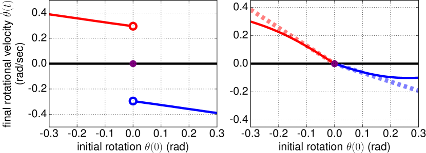
Figure 1: Trajectory outcomes in mechanical systems subject to unilateral constraints. (left) In general, trajectory outcomes depend discontinuously on initial conditions. In the pictured model for rigid–leg trotting (adapted from [26]), discontinuities arise when two legs touch down: if the legs impact simultaneously (corresponding to rotation $\theta(0)=0$), then the post–impact rotational velocity is zero; if the left leg impacts before the right leg ($\theta(0)>0$, blue) or vice–versa ($\theta(0)<0$, red), then the post–impact rotational velocities are bounded away from zero. (right) In the pictured model for soft–leg trotting (adapted from [6] with the addition of a nonlinear damper coupling the body and limbs), trajectory outcomes (solid lines) are continuous and piecewise–differentiable at $\theta(0)=0$ (dashed lines).

Specifically, this paper provides mathematical conditions on mechanical systems subject to unilateral constraints that ensure trajectory outcomes vary continuously and piecewise–differentiably with respect to initial conditions. Conditions that ensure continuity are known; see for instance Schatzman’s work on the one–dimensional impact problem [30] or Ballard’s seminal result [2, Thm. 20]. Furthermore, when the sequence of constraint activations and deactivations is held fixed, it has been known for some time that outcomes depend differentiably on initial conditions; see [1] for the earliest instance of this result we found in the English literature and [13, 10, 34, 7] for modern treatments. Our contribution is a proof that imposing an additional admissibility condition ensures continuous trajectory outcomes are piecewise–differentiable with respect to initial conditions, even as the sequence of constraint activations and deactivations varies; see Fig. 1 (right). The operative notion of piecewise–differentiability was originally developed by the nonsmooth analysis community to study structural stability of nonlinear programs [28], and now forms the basis of a rather complete generalization of Calculus accommodating non–linear first–order approximations [31]. In the terminology of that community, we provide conditions that ensure the flow of a mechanical system subject to unilateral constraints is $PC^{r}$, and therefore possesses a piecewise–linear Bouligand (or B–)derivative.

As discussed in more detail in Sec. 6, we envision the existence and straightforward computability of the B–derivative of the flow to be useful in practice because it supports generalization of familiar control techniques to a class of hybrid systems with physical significance. In particular, building on related work that dealt with differential equations with discontinuous right–hand–sides [5, 4], our B–derivative can be used to assess stability, controllability, or optimality of trajectories in mechanical systems subject to unilateral constraints. As control of dynamic and dexterous robots increasingly relies on scalable algorithms for optimization and learning that presume the existence of first–order approximations (i.e. gradients or gradient–like objects) [24, 17, 21, 18], it is important to place application of such algorithms on a firm theoretical foundation. From a theoretical perspective, the results in this paper dovetail with recent advances in simulation of hybrid systems [6] in that one of the conditions necessary for the B–derivative to exist (namely, continuity of trajectory outcomes) is also requisite for convergence of numerical simulations. Taken together, these observations suggest that a unified analytical and computational framework for modeling and control of mechanical systems subject to unilateral constraints may be within reach.

1.1 Organization

We begin in Sec. 2 by specifying the class of dynamical systems under consideration, namely, mechanical systems subject to unilateral constraints. Sec. 3 summarizes the well–known fact that, when the contact mode sequence is fixed, trajectories vary differentiably with respect to initial conditions. In Sec. 4, we observe (as others have) that trajectories generally vary discontinuously with respect to initial conditions as the contact mode sequence varies, but provide a sufficient condition that is known to restore continuity. Sec. 5 leverages continuity to provide conditions under which trajectories vary piecewise–differentiably with respect to initial conditions across contact mode sequences, and Sec. 6 discusses extensions and implications for a systems theory for mechanical systems subject to unilateral constraints.

1.2 Relation to prior work

The technical content in Sec. 2, Sec. 3, and Sec. 4 appeared previously in the literature and is (more–or–less) well–known; we collate the results here in a sequence of technical Lemmas to contextualize our contributions in Sec. 5.

2 Mechanical systems subject to unilateral constraints

In this paper, we study the dynamics of a mechanical system with configuration coordinates $q\in Q=\mathbb{R}^{d}$ subject to (perfect, holonomic, scleronomic) unilateral constraints $a(q)\geq 0$ specified by a differentiable function $a\colon Q\rightarrow\mathbb{R}^{n}$ where $d,n\in\mathbb{N}$ are finite. We are primarily interested in systems with $n>1$ constraints, whence we regard the inequality $a(q)\geq 0$ as being enforced componentwise. Given any $J\subset\left\{1,\dots,n\right\}$, and letting $\left|J\right|$ denote the number of elements in the set $J$, we let $a_{J}\colon Q\rightarrow\mathbb{R}^{\left|J\right|}$ denote the function obtained by selecting the component functions of $a$ indexed by $J$, and we regard the equality $a_{J}(q)=0$ as being enforced componentwise. It is well–known (see e.g. [2, Sec. 3] or [15, Sec. 2.4, 2.5]) that with $J=\left\{j\in\left\{1,\dots,n\right\}:a_{j}(q)=0\right\}$ the system’s dynamics take the form

$$M(q)\ddot{q} =f(q,\dot{q})+c(q,\dot{q})\dot{q}+Da_{J}(q)^{\top}\lambda_{J}(q,\dot{q}),$$ (1a)

$$\dot{q}^{+} =\Delta_{J}(q,\dot{q}^{-})\dot{q}^{-},$$ (1b)

where $M\colon Q\rightarrow\mathbb{R}^{d\times d}$ specifies the mass matrix (or inertia tensor) for the mechanical system in the $q$ coordinates, $f\colon TQ\rightarrow\mathbb{R}^{d}$ is termed the effort map [2] and specifies the internal and applied forces, $c\colon TQ\rightarrow\mathbb{R}^{d\times d}$ denotes the Coriolis matrix determined by $M$, $Da_{J}\colon Q\rightarrow\mathbb{R}^{\left|J\right|\times d}$ denotes the (Jacobian) derivative of the constraint function $a_{J}$ with respect to the coordinates, $\lambda_{J}\colon TQ\rightarrow\mathbb{R}^{\left|J\right|}$ denotes the reaction forces generated in contact mode $J$ to enforce the constraint $a_{J}(q)\geq 0$, $\Delta_{J}\colon TQ\rightarrow\mathbb{R}^{d\times d}$ specifies the collision restitution law that instantaneously resets velocities to ensure compatibility with the constraint $a_{J}(q)=0$,

$$\Delta_{J}(q,\dot{q})= I_{d}-(1+\gamma(q,\dot{q}))M(q)^{-1}Da_{J}(q)^{\top}\Lambda_{J}(q)Da_{J}(q),$$ (2)

where $I_{d}$ is the $d$–dimensional identity matrix, $\gamma\colon TQ\rightarrow[0,\infty)$ specifies the coefficient of restitution, $\dot{q}^{+}$ (resp. $\dot{q}^{-}$) denotes the right– (resp. left–)handed limits of the velocity vector with respect to time, and $\Lambda_{J}\colon Q\rightarrow R^{d\times d}$

$$\Lambda_{J}(q)=\left(Da_{J}(q)M(q)^{-1}Da_{J}(q)^{\top}\right)^{-1}.$$ (3)

Definition 1 (contact modes)

With
$A=\left\{q\in Q:a(q)\geq 0\right\}$ denoting the set of admissible configurations, the constraint functions $\left\{a_{j}\right\}_{j=1}^{n}$ partition $A$ into a finite collection $\left\{A_{J}\right\}_{J\in 2^{n}}$ of contact modes:

$$\forall J\in 2^{n}:A_{J}=\left\{q\in Q\mid\right. a_{J}(q)=0,$$ (4)

$$\left.\forall i\not\in J:a_{i}(q)>0\right\}.$$

We let $TA=\left\{(q,\dot{q})\in TQ:q\in A\right\}$ and
$TA_{J}=\left\{(q,\dot{q})\in TQ:q\in A_{J}\right\}$ for each $J\in 2^{n}$.

Remark 1

In Def. 1 (contact modes), $J=\left\{1,\dots,n\right\}$ indexes the maximally constrained contact mode and $J=\emptyset$ indexes the unconstrained contact mode. Since any velocity is allowable in the unconstrained mode, we adopt the convention $\Delta_{\emptyset}(q,\dot{q})=I_{d}$.

In the present paper, we will assume that appropriate conditions have been imposed to ensure trajectories of (1) exist on a region of interest in time and state.

Assumption 1 (existence and uniqueness)

There exists a flow for (1), that is, a function $\phi:\mathscr{F}\rightarrow TA$ where $\mathscr{F}\subset[0,\infty)\times TA$ is an open subset containing $\left\{0\right\}\times TA$ and for each $(t,(q,\dot{q}))\in\mathscr{F}$ the restriction $\phi|_{[0,t]\times\left\{(q,\dot{q})\right\}}:[0,t]\rightarrow TQ$ is the unique left–continuous trajectory for (1) initialized at $(q,\dot{q})$.

Remark 2

The problem of ensuring trajectories of (1) exist and are unique has been studied extensively; we refer the reader to [2, Thm. 10] for a specific result and [15] for a general discussion of this problem.

Since we are concerned with differentiability properties of the flow, we assume the elements in (1) are differentiable.

Assumption 2 ($C^{r}$ vector field and reset map)

The vector field (1a) and reset map (1b) are continuously differentiable to order $r\in\mathbb{N}$.

Remark 3

If we restricted our attention to the continuous–time dynamics in (1), then Assump. 2 would suffice to provide the local existence and uniqueness of trajectories imposed by Assump. 1; as illustrated by [2, Ex. 2], Assump. 2 does not suffice when the vector field (1a) is coupled to the reset map (1b).

3 Differentiability within contact mode sequences

It is possible to satisfy Assump. 1 (existence and uniqueness of flow) under mild conditions that allow trajectories to exhibit phenomena such as grazing (wherein the trajectory activates a new constraint without undergoing impact) or Zeno (wherein the trajectory undergoes an infinite number of impacts in a finite time interval). In this and subsequent sections, where we seek to study differentiability properties of the flow, we will not be able to accommodate grazing or Zeno phenomena. Therefore we proceed to restrict the trajectories under consideration.

Definition 2 (constraint activation/deactivation)

The trajectory $\phi^{(q,\dot{q})}$ initialized at $(q,\dot{q})\in TA_{J}\subset TQ$ activates constraints $I\in 2^{n}$ at time $t>0$ if (i) no constraint in $I$ was active immediately before time $t$ and (ii) all constraints in $I$ become active at time $t$. Formally,

$$\exists\varepsilon>0:\ I\cap J=\emptyset,\ \text{(i)} \phi\left((t-\varepsilon,t),(q,\dot{q})\right)\subset TA_{J},$$ (5)

(ii) $$\phi(t,(q,\dot{q}))\in TA_{I\cup J}.$$

We refer to $t$ as a constraint activation time for $\phi^{(q,\dot{q})}$. Similarly, the trajectory $\phi^{(q,\dot{q})}$ deactivates constraints $I\in 2^{n}$ at time $t>0$ if (i) all constraints in $I$ were active at time $t$ and (ii) no constraint in $I$ remains active immediately after time $t$. Formally,

$$\exists\varepsilon>0:\ I\subset J,\ \text{(i)} \phi(t,(q,\dot{q}))\in TA_{J},$$ (6)

(ii) $$\phi\left((t,t+\varepsilon),(q,\dot{q})\right)\subset TA_{J\setminus I}.$$

We refer to $t$ as a constraint deactivation time for $\phi^{(q,\dot{q})}$.

Definition 3 (admissible activation/deactivation)

A constraint activation time $t>0$ for $\phi^{(q,\dot{q})}$ is admissible if the constraint velocity for all activated constraints $I\in 2^{n}$ is negative. Formally, with $(\rho,\dot{\rho}^{-})=\lim_{s\rightarrow t^{-}}\phi(s,(q,\dot{q}))$ denoting the left–handed limit of the trajectory at time $t$,

$$\forall i\in I:D_{t}\left[a_{i}\circ\phi\right](0,(\rho,\dot{\rho}^{-}))=Da_{i}(\rho)\dot{\rho}^{-}<0.$$ (7)

A constraint deactivation time $t>0$ for $\phi^{(q,\dot{q})}$ is admissible if, for all deactivated constraints $I\in 2^{n}$: (i) the constraint velocity or constraint acceleration is positive, or (ii) the time derivative of the contact force is negative. Formally, with $(\rho,\dot{\rho}^{+})=\lim_{s\rightarrow t^{+}}\phi(s,(q,\dot{q}))$ denoting the right–handed limit of the trajectory at time $t$, for all $i\in I:$

$$\text{(i)}\ D_{t}\left[a_{i}\circ\phi\right](0,(\rho,\dot{\rho}^{+})) >0\ \text{or}$$ (8)

$$D^{2}_{t}\left[a_{i}\circ\phi\right](0,(\rho,\dot{\rho}^{+})) >0,$$

$$\text{or (ii)}\ D_{t}\left[\lambda_{i}\circ\phi\right](0,(\rho,\dot{\rho}^{+})) <0.$$

Remark 4

The conditions for admissible constraint deactivation in case (i) of (8) can only arise at admissible constraint activation times; otherwise the trajectory is continuous, whence active constraint velocities and accelerations are zero.

Definition 4 (admissible trajectory)

A trajectory $\phi^{(q,\dot{q})}$ is admissible on $[0,t]\subset\mathbb{R}$ if (i) it has a finite number of constraint activation (hence, deactivation) times on $[0,t]$, and (ii) every constraint activation and deactivation is admissible; otherwise the trajectory is inadmissible.

Remark 5 (admissible trajectories)

The key property admissible trajectories possess that will be leveraged in what follows is: time–to–activation and time–to–deactivation are differentiable with respect to initial conditions; the same is not generally true of inadmissible trajectories.

Remark 6 (grazing is not admissible)

The restriction in Def. 4 (admissible trajectory) that all constraint activation/deactivation times are admissible precludes admissibility of grazing.

Remark 7 (Zeno is not admissible)

The restriction in Def. 4 (admissible trajectory) that a finite number of constraint activations occur on a compact time interval precludes admissibility of Zeno.

Definition 5 (contact mode sequence)

The contact mode sequence associated with a trajectory $\phi^{(q,\dot{q})}$ that is admissible on $[0,t]\subset\mathbb{R}$ is the unique function $\omega\colon\left\{0,\dots,m\right\}\rightarrow 2^{n}$ such that there exists a finite sequence of times $\left\{t_{\ell}\right\}_{\ell=0}^{m+1}\subset[0,t]$ for which $0=t_{0}<t_{1}<\cdots<t_{m+1}=t$ and

$$\forall\ell\in\left\{0,\dots,m\right\}:\phi((t_{\ell},t_{\ell+1}),(q,\dot{q}))\subset TA_{\omega(\ell)}.$$ (9)

Remark 8

In Def. 8 (contact mode sequence), the sequence $\omega$ is easily seen to be unique by the admissibility of the trajectory; indeed, the associated time sequence consists of start, stop, and constraint activation/deactivation times.

Assumption 3 (independent constraints)

The constraints are independent:

$$\forall J\in 2^{n},\ q\in a_{J}^{-1}(0): \left\{Da_{j}(q)\right\}_{j\in J}\subset T^{*}_{q}Q$$ (10)

$$\quad\text{is linearly independent}.$$

Remark 9

Algebraically, Assump. 3 (independent constraints) implies that the constraint forces $\lambda_{J}$ are well–defined, and that there are no more constraints than degrees–of–freedom, $n\leq d$. Geometrically, it implies for each $J\in 2^{n}$ that $a_{J}^{-1}(0)\subset Q$ is an embedded codimension–$\left|J\right|$ submanifold, and that the codimension–1 submanifolds $\left\{a_{j}^{-1}(0)\right\}_{j\in J}$ intersect transversally; this follows from [19, Thm. 5.12] since each $a_{J}\colon Q\rightarrow\mathbb{R}$ must be constant–rank on its zero section.

We now state the well–known fact that, if the contact mode sequence is fixed, then admissible trajectory outcomes are differentiable with respect to initial conditions.

Lemma 1 (differentiability within mode seq. [1])

Under Assump. 1 (existence and uniqueness of flow), Assump. 2 ($C^{r}$ vector field and reset map), and Assump. 3 (independent constraints), with $\phi\colon[0,\infty)\times TA\rightarrow TA$ denoting the flow, if $\Sigma\subset TQ$ is a $C^{r}$ embedded submanifold such that all trajectories initialized in $\Sigma\cap TA$

1. are admissible on $[0,t]\subset\mathbb{R}$ and

2. have the same contact mode sequence,

then the restriction $\phi|_{\left\{t\right\}\times\Sigma}$ is $C^{r}$.

4 (Dis)continuity across contact mode sequences

As stated in Sec. 1, the point of this paper is to provide sufficient conditions that ensure trajectories of (1) vary differentiably as the contact mode sequence varies. A precondition for differentiability is continuity, whence in this section we consider what condition must be imposed to give rise to continuity in general. We begin in Sec. 4.1 by demonstrating that the transversality of constraints imposed by Assump. 3 (independent constraints) generally gives rise to discontinuity, then introduce an orthogonality condition in Sec. 4.2 that suffices to restore continuity.

4.1 Discontinuity across contact mode sequences

Consider an unconstrained initial condition $(q,\dot{q})\in TA_{\emptyset}\subset TQ$ that impacts (i.e. admissibly activates) exactly two constraints $i,j\in\left\{1,\dots,n\right\}$ at time $t>0$; with $(\rho,\dot{\rho}^{-})=\phi(t,(q,\dot{q}))$ we have

$$a_{\left\{i,j\right\}}(\rho)=0,\ Da_{i}(\rho)\dot{\rho}^{-}<0,\ Da_{j}(\rho)\dot{\rho}^{-}<0.$$ (11)

The pre–impact velocity $\dot{\rho}^{-}$ abruptly resets via (1b):

$$\dot{\rho}^{+}=\Delta_{\left\{i,j\right\}}(\rho)\dot{\rho}^{-}.$$ (12)

As noted in Remark 9 (independent constraints), the constraint surfaces $a_{i}^{-1}(0)$, $a_{j}^{-1}(0)$ intersect transversally. Therefore given any $\varepsilon>0$ it is possible to find $(q_{i},\dot{q}_{i})$ and $(q_{j},\dot{q}_{j})$ in the open ball of radius $\varepsilon$ centered at $(q,\dot{q})$ such that the trajectory $\phi^{(q_{i},\dot{q}_{i})}$ impacts constraint $i$ before constraint $j$ and $\phi^{(q_{j},\dot{q}_{j})}$ impacts $j$ before $i$. As $\varepsilon>0$ tends toward zero, the time spent flowing according to (1a) tends toward zero, hence the post–impact velocities tend toward the twofold iteration of (1b):

$$\dot{\rho}_{i}^{+}=\Delta_{\left\{i,j\right\}}(\rho)\Delta_{i}(\rho)\dot{\rho}^{-},$$ (13)

$$\dot{\rho}_{j}^{+}=\Delta_{\left\{i,j\right\}}(\rho)\Delta_{j}(\rho)\dot{\rho}^{-}.$$

Recalling for all $J\in 2^{n}$ that $\Delta_{J}\in\mathbb{R}^{d\times d}$ is an orthogonal projection onto the tangent plane of the codimension–$\left|J\right|$ submanifold $a_{J}^{-1}(0)$, observe that $\dot{\rho}_{i}^{+}=\dot{\rho}^{+}=\dot{\rho}_{j}^{+}$ if and only if $Da_{i}(\rho)$ is orthogonal to $Da_{j}(\rho)$. Therefore if constraints intersect transversally but non–orthogonally, outcomes from the dynamics in (1) vary discontinuously as the contact mode sequence varies.

Remark 10 (discontinuous locomotion outcomes)

The analysis of a saggital–plane quadruped in [26] provides an instructive example of the behavioral consequences of transverse but non–orthogonal constraints in a model of legged locomotion. As summarized in [26, Table 2], the model possesses 3 distinct but nearby trot (or trot–like) gaits, corresponding to whether two legs impact simultaneously (as in (12)) or at different time instants (as in (13)); the trot that undergoes simultaneous impact is unstable due to discontinuous dependence of trajectory outcomes on initial conditions.

4.2 Continuity across contact mode sequences

To preclude the discontinuous dependence on initial conditions exhibited in Sec. 4.1, we strengthen the transversality of constraints implied by Assump. 3 (independent constraints) by imposing orthogonality of constraints.

Assumption 4 (orthogonal constraints)

Constraint surfaces intersect orthogonally:

$$\forall i,j\in\left\{1,\dots,n\right\},\ i\neq j,\ q\in a_{i}^{-1}(0)\cap a_{j}^{-1}(0):$$ (14)

$$\langle Da_{i}(q),Da_{j}(q)\rangle_{M^{-1}}=0.$$

Remark 11

Note that Assump. 4 (orthogonal constraints) is strictly stronger than Assump. 3 (independent constraints). Physically, the assumption can be interpreted as asserting that any two independent limbs that can undergo impact simultaneously must be inertially decoupled. This can be achieved in artifacts by introducing series compliance in a sufficient number of degrees–of–freedom.

Sec. 4.1 demonstrated that Assump. 4 (orthogonal constraints) is necessary in general to preclude discontinuous dependence on initial conditions. The following result demonstrates that this assumption is sufficient to ensure continuous dependence on initial conditions.

Lemma 2 (continuity across mode seq. [2, Thm. 20])

Under Assump. 1 (existence and uniqueness of flow), Assump. 2 ($C^{r}$ vector field and reset map), and Assump. 4 (orthogonal constraints), with $\phi\colon[0,\infty)\times TA\rightarrow TA$ denoting the flow, if $t\in\mathbb{R}$ and $(p,\dot{p})\in TA\subset TQ$ are such that $t$ is not a constraint activation time for $(p,\dot{p})$, then $\phi$ is continuous at $(t,(p,\dot{p}))$.

Remark 12 (continuity across mode seq.)

The preceding result implies that the flow $\phi$ is continuous almost everywhere in both time and state, without needing to restrict to admissible trajectories. Thus orthogonal constraints ensure the flow $\phi$ depends continuously on initial conditions, even along trajectories that exhibit grazing and Zeno phenomena. For the reason described in Remark 5 (admissible trajectories), we will not be able to accommodate these phenomena when we study differentiability properties of trajectories in the next section.

5 Differentiability across contact mode sequences

We now provide conditions that ensure trajectories depend differentiably on initial conditions, even as the contact mode sequence varies. In general, the flow does not possess a classical Jacobian (alternately called Fréchet or F–)derivative, i.e. there does not exist a single linear map that provides a first–order approximation for the flow. Instead, under the admissibility conditions introduced in Sec. 3, we show that the flow admits a piecewise–linear first–order approximation termed a Bouligand (or B–)derivative [31, Ch. 3.1]. Though perhaps unfamiliar, this derivative is nevertheless quite useful. Significantly, unlike functions that are merely directionally differentiable, B–differentiable functions admit generalizations of many techniques familiar from calculus, including the Chain Rule [31, Thm 3.1.1] (and hence Product and Quotient Rules [31, Cor. 3.1.1]), Fundamental Theorem of Calculus [31, Prop. 3.1.1], and Implicit Function Theorem [31, Thm. 4.2.3], and the B–derivative can be employed to implement scalable algorithms [16] for optimization or learning.

We proceed by showing that the flow is piecewise–differentiable in the sense defined in [31, Ch. 4.1] and recapitulated here; functions that are piecewise–differentiable in this sense are always B–differentiable [31, Prop. 4.1.3]. Let $r\in\mathbb{N}\cup\left\{\infty\right\}$ denote an order of differentiability and $D\subset\mathbb{R}^{m}$ be open. A continuous function $\psi\colon D\rightarrow\mathbb{R}^{\ell}$ is called piecewise–$C^{r}$ if the graph of $\psi$ is everywhere locally covered by the graphs of a finite collection of functions that are $r$ times continuously differentiable ($C^{r}$–functions). Formally, for every $x\in D$ there must exist an open set $U\subset D$ containing $x$ and a finite collection $\left\{\psi_{\omega}\colon U\rightarrow\mathbb{R}^{\ell}\right\}_{\omega\in\Omega}$ of $C^{r}$–functions such that for all $x\in U$ we have $\psi(x)\in\left\{\psi_{\omega}(x)\right\}_{\omega\in\Omega}$.

We now state and prove the main result of this paper: whenever the flow of a mechanical system subject to unilateral constraints is continuous and admissible, it is piecewise–$C^{r}$; see Fig. 2 for an illustration.

Theorem 1 (piecewise–differentiable flow)

Under Assump. 1 (existence and uniqueness of flow), Assump. 2 ($C^{r}$ vector field and reset map), and Assump. 4 (orthogonal constraints), with $\phi\colon[0,\infty)\times TA\rightarrow TA$ denoting the flow, if $t\in[0,\infty)$, $(p,\dot{p})\in TA\subset TQ$, and $\Sigma\subset TQ$ is a $C^{r}$ embedded submanifold containing $(p,\dot{p})$ such that

1. the trajectory $\phi^{(p,\dot{p})}$ activates and/or deactivates constraints at time $s\in(0,t)$,

2. $\phi^{(p,\dot{p})}$ has no other activation or deactivation times in $[0,t]$,

3. trajectories initialized in $\Sigma\cap TA$ are admissible on $[0,t]$, and

4. the set $\Omega$ of contact mode sequences for trajectories initialized in $\Sigma\cap TA$ is finite,

then the restriction $\phi|_{[0,\infty)\times\Sigma}$ is piecewise–$C^{r}$ at $(t,(p,\dot{p}))$.

Proof 5.2.

We seek to show that the restriction $\phi|_{[0,\infty)\times\Sigma}$ is piecewise–$C^{r}$ at $(t,(p,\dot{p}))$. We will proceed by constructing a finite set of $r$ times continuously differentiable selection functions for $\phi$ on $[0,t]\times\Sigma$. In the example given in Fig. 2, there are two selection functions, one corresponding to a perturbation along $(v_{r},\dot{v}_{r})$, colored red, and the other along $(v_{b},\dot{v}_{b})$, colored blue. These selection functions will be indexed by a pair of functions $(\omega,\eta)$ where: $\omega\colon\left\{0,\dots,m\right\}\rightarrow 2^{n}$ is a contact mode sequence, i.e. $\omega\in\Omega$; $\eta\colon\left\{0,\dots,m-1\right\}\rightarrow\left\{1,\dots,n\right\}$ indexes constraints that undergoes admissible activation or deactivation at the contact mode transition indexed by $\ell\in\left\{0,\dots,m-1\right\}$. For instance, in Fig. 2 the index functions for the (de)activation sequence starting from $(v_{r},\dot{v}_{r})$, in red, are $\omega_{r}(0)=\left\{1\right\},\omega_{r}(1)=\emptyset,\omega_{r}(2)=\left\{2\right\}$, $\eta_{r}(1)=1,\eta_{r}(2)=2$, and the index functions for the (de)activation sequence starting from $(v_{b},\dot{v}_{b})$, in blue, are $\omega_{b}(0)=\left\{1\right\},\omega_{b}(1)=\left\{1,2\right\},\omega_{b}(2)=\left\{2\right\}$, $\eta_{b}(1)=2,\eta_{b}(2)=1$. Note that for each $\omega\in\Omega$ the set $H(\omega)$ of possible $\eta$’s is finite; since the set $\Omega$ is finite by assumption, the set of pairs $(\omega,\eta)$ is finite.

Let $(\omega\colon\left\{0,\dots,m\right\}\rightarrow 2^{n})\in\Omega$ and $(\eta\colon\left\{0,\dots,m-1\right\}\rightarrow\left\{1,\dots,n\right\})\in H(\omega)$ be as described above. Let $\mu\colon\left\{0,\dots,m\right\}\rightarrow 2^{n}$ be defined as $\mu(k)=\bigcup_{i=0}^{k-1}\left\{\eta(i)\right\}$, where we adopt the convention that $\bigcup_{i=0}^{-1}\left\{i\right\}=\emptyset$; note that $\mu$ is uniquely determined by $\eta$. For the sake of readability, we suppress dependence on $\eta$ and $\omega$ until (21). Let $(\rho,\dot{\rho}^{-})=\lim_{u\uparrow s}\phi(u,(p,\dot{p}))$. For all $k\in\left\{0,\dots,m\right\}$ define $\dot{\rho}_{k}=\Delta_{\mu(k)}(\rho)\dot{\rho}^{-}$. There exists an open neighborhood $U_{k}\subset TQ$ containing $(\rho,\dot{\rho}_{k})$ such that the vector field determined by (1a) at $\omega(k)$ admits a $C^{r}$ extension to $F_{k}\colon U_{k}\rightarrow\mathbb{R}^{2d}$. (Note that for $k=m$ (resp. $k=0$) the neighborhood $U_{k}$ can be taken to additionally include $\phi((s,t],(p,\dot{p}))$ (resp. $\phi([0,s),(p,\dot{p}))$).)

By the Fundamental Theorem on Flows [19, Thm. 9.12], $F_{k}$ determines a unique maximal flow $\phi_{k}\colon\mathscr{F}_{k}\rightarrow U_{k}$ over a maximal flow domain $\mathscr{F}_{k}\subset\mathbb{R}\times U_{k}$, which is an open set that contains $\left\{0\right\}\times U_{k}$, and the flow $\phi_{\ell}$ is $C^{r}$. (Note that $(t-s,(\rho,\dot{\rho}_{m}))\in\mathscr{F}_{m}$ and $(s,(p,\dot{p}))\in\mathscr{F}_{0}$.)

If $\eta(\ell)$ indexes an admissible constraint activation (recall that $\ell\in\left\{0,\dots,m-1\right\}$), then there exists a time–to–activation $\tau_{\ell}\colon U_{\ell}\rightarrow\mathbb{R}$ defined over an open set $U_{\ell}\subset TQ$ containing $(\rho,\dot{\rho}_{\ell})$ such that

$$\forall(q,\dot{q})\in U_{\ell}:a_{\eta(\ell)}\circ\phi_{\ell}(\tau_{\ell}(q,\dot{q}),(q,\dot{q}))=0.$$ (15)

If instead $\eta(\ell)$ indexes an admissible constraint deactivation, then there exists a time–to–deactivation $\tau_{\ell}\colon U_{\ell}\rightarrow\mathbb{R}$ defined over an open set $U_{\ell}\subset TQ$ containing $(\rho,\dot{\rho}_{\ell})$ such that

$$\forall(q,\dot{q})\in U_{\ell}:\lambda_{\eta(\ell)}\circ\phi_{\ell}(\tau_{\ell}(q,\dot{q}),(q,\dot{q}))=0.$$ (16)

In either case, $\tau_{\ell}$ exists and is $C^{r}$ by the Implicit Function Theorem [19, Thm. C.40] due to admissibility of trajectories initialized in $\Sigma$. (Note for $\ell=0$ the neighborhood $U_{\ell}$ can be extended to include $\phi([0,s),(p,\dot{p}))$ using the semi–group property of the flow $\phi_{\ell}$.) See Fig. 2 for an illustration of constraint activations and deactivations.

Let $\varphi_{\ell}\colon\mathbb{R}\times U_{\ell}\rightarrow\mathbb{R}\times U_{\ell}$ be defined for all $(u,(q,\dot{q}))\in\mathbb{R}\times U_{\ell}$ by

$$\varphi_{\ell}(u,(q,\dot{q}))=\left(u-\tau_{\ell}(q,\dot{q}),\phi_{\ell}\left(\tau_{\ell}(q,\dot{q}),(q,\dot{q})\right)\right).$$ (17)

The map $\varphi_{\ell}$ flows a state $(q,\dot{q})$ using the vector field from contact mode $\omega(\ell)$ until constraint $\eta(\ell)$ undergoes admissible activation/deactivation, and deducts the time required from the given budget $u$. The total derivative of $\varphi_{\ell}$ at $(0,(\rho,\dot{\rho}_{\ell}))$ (see also [5, § 7.1.4]) is

$$D\varphi_{\ell}(0,(\rho,\dot{\rho}_{\ell}))=\left[\begin{array}[]{cc}1&\frac{1}{gf}g\\ 0&I_{2d}-\frac{1}{gf}fg\end{array}\right],$$ (18)

where $f=F(\rho,\dot{\rho}_{\ell})$ and $g=Dh_{\eta(\ell)}(\rho,\dot{\rho}_{\ell})$ where $h_{\ell}\colon TQ\rightarrow\mathbb{R}$ is defined for all $(q,\dot{q})\in TQ$ by $h_{\ell}(q,\dot{q})=a_{\eta(\ell)}(q)$.

Let $\Gamma_{\ell}\colon\mathbb{R}\times TQ\rightarrow\mathbb{R}\times TQ$ be defined for all $(u,(q,\dot{q}))\in\mathbb{R}\times TQ$ by

$$\Gamma_{\ell}(u,(q,\dot{q}))=(u,(q,\Delta_{\mu(\ell)}(q)\dot{q})).$$ (19)

The map $\Gamma_{\ell}$ resets velocities to be compatible with contact mode $\omega(\ell)$ while leaving positions and times unaffected. The total derivative of $\Gamma_{\ell}$ at $(u,(q,\dot{q}))$ is given by

$$D\Gamma_{\ell}(u,(q,\dot{q}))=\left[\begin{array}[]{ccc}1&0&0\\ 0&I_{d}&0\\ 0&D_{q}(\Delta_{\mu(\ell)}(q)\dot{q})&\Delta_{\mu(\ell)}(q)\end{array}\right].$$ (20)

For each $\omega\in\Omega$ and $\eta\in H(\omega)$ define $\phi_{\omega}^{\eta}$ by the formal composition

$$\phi_{\omega}^{\eta}=\phi_{m}\circ\prod_{\ell=0}^{m-1}\left(\Gamma_{\ell+1}\circ\varphi_{\ell}\right).$$ (21)

We take as the domain of $\phi_{\omega}^{\eta}$ the set

$$\mathscr{F}_{\omega}^{\eta}=\left(\phi_{\omega}^{\eta}\right)^{-1}(TQ)\subset\mathbb{R}\times TQ,$$ (22)

noting that $\mathscr{F}_{\omega}^{\eta}$ is (i) open since each function in the composition is continuous, and (ii) nonempty since $(t,(p,\dot{p}))\in\mathscr{F}_{\omega}^{\eta}$. The map $\phi_{\omega}^{\eta}$ flows states via a given contact mode sequence for a specified amount of time; note that some of the resulting “trajectories” are not physically realizable, as they may evaluate the flows $\left\{\phi_{k}\right\}_{k=0}^{m}$ in backward time. An example of such a physically unrealizable “trajectory” is illustrated in Fig. 2 by $\phi_{\eta_{r}}^{\omega_{r}}(t,(v_{b},\dot{v}_{b}))$, which first flows forward in time via the extended vector field $F_{\left\{1\right\}}$ past the constraint surface $\left\{a_{2}(q)=0\right\}$ until constraint 1 deactivates and then flows backwards in time until constraint 2 activates, ultimately terminating in $TA_{\left\{2\right\}}$.

With $\mathscr{F}=\bigcap\left\{\mathscr{F}_{\omega}^{\eta}:\omega\in\Omega,\eta\in H(\omega)\right\}\subset[0,\infty)\times TQ$, for any $(u,(q,\dot{q}))\in\mathscr{F}\cap\left([0,\infty)\times TA\right)$ with contact mode sequence $\omega\in\Omega$ and constraint sequence $\eta\in H(\omega)$, the trajectory outcome is obtained by applying $\phi_{\omega}^{\eta}$ to $(u,(q,\dot{q}))$, i.e. $\phi(u,(q,\dot{q}))=\phi_{\omega}^{\eta}(u,(q,\dot{q}))$. See Fig. 2 for an illustration of trajectories with different contact mode sequences.

The maps $\varphi_{\ell}$, $\Gamma_{\ell}$, and $\phi_{\omega}^{\eta}$ are $C^{r}$ on their domains since they are each obtained from a finite composition of $C^{r}$ functions. Therefore the restriction $\phi|_{[0,\infty)\times\Sigma}$ is a continuous selection of the finite collection of $C^{r}$ functions

$$\left\{\phi_{\omega}^{\eta}:\omega\in\Omega,\eta\in H(\omega)\right\}$$

on the open neighborhood $\mathscr{F}\subset TQ$ containing $(t,(p,\dot{p}))$, i.e. $\phi|_{[0,\infty)\times\Sigma}$ is piecewise–$C^{r}$ at $(t,(p,\dot{p}))$. See Fig. 2 for an illustration the piecewise–differentiability of trajectory outcomes arising from a transition between contact mode sequences.

Remark 5.3 (relaxing Theorem hypotheses).

Since the class of piecewise–differentiable functions is closed under finite composition, conditions (i) and (ii) in the preceding Theorem can be readily relaxed to accommodate a finite number of constraint activation/deactivation times in the interval $(0,t)$. Conditions (iii) and (iv) are more difficult to relax since there are systems wherein trajectories initialized arbitrarily close to an admissible trajectory fail to be admissible themselves. As a familiar example, consider a 1 degree–of–freedom elastic impact oscillator [11, Ch. 2.4] (i.e. a bouncing ball): the stationary trajectory (initialized with $q,\dot{q}=0$) is admissible for all time, but all nearby trajectories (initialized with $q\neq 0$ or $\dot{q}\neq 0$) exhibit the Zeno phenomenon. We will discuss further possible extensions in Sec. 6.1.1.

Figure 2: Illustration of trajectory undergoing simultaneous constraint activation and deactivation: the trajectory initialized at $(p,\dot{p})\in TA_{\left\{1\right\}}\subset TQ$ flows via (1a) to a point $(\rho,\dot{\rho}^{-})\in TA_{\left\{1\right\}}$ where both the constraint force $\lambda_{1}$ and constraint function $a_{2}$ are zero, instantaneously resets velocity via (1b) to $\dot{\rho}^{+}=\Delta_{\left\{2\right\}}(\rho)\dot{\rho}^{-}$, then flows via (1a) to $\phi(t,(p,\dot{p}))\in TA_{\left\{2\right\}}\subset TQ$. Nearby trajectories undergo activation and deactivation at distinct times: trajectories initialized in the red region, e.g. $(v_{r},\dot{v}_{r})$, deactivate constraint $1$ and flow through contact mode $TA_{\emptyset}$ before activating constraint $2$—their contact mode sequence is $\left(\left\{1\right\},\emptyset,\left\{2\right\}\right)$—while trajectories initialized in the blue region, e.g. $(v_{b},\dot{v}_{b})$, activate $2$ and flow through $TA_{\left\{1,2\right\}}$ before deactivating $1$—their contact mode sequence is $\left(\left\{1\right\},\left\{1,2\right\},\left\{2\right\}\right)$. Piecewise–differentiability of the trajectory outcome is illustrated by the fact that red outcomes lie along a different subspace than blue.

Under the hypotheses of the preceding Theorem, the continuous flow $\phi$ is piecewise–differentiable at a point $(t,(p,\dot{p}))\in[0,\infty)\times TA$, that is, near $(t,(p,\dot{p}))$ the graph of $\phi$ is covered by the graphs of a finite collection $\left\{\phi_{\omega}^{\eta}:\omega\in\Omega,\eta\in H(\omega)\right\}$ of differentiable functions (termed selection functions). This implies in particular that there exists a continuous and piecewise–linear function

$$D\phi(t,(p,\dot{p})):T_{(t,(p,\dot{p}))}\left([0,\infty)\times TA\right)\rightarrow T_{\phi(t,(p,\dot{p}))}A$$ (23)

(termed the Bouligand or B–derivative) that provides a first–order approximation for how trajectory outcomes vary with respect to initial conditions. Formally, for all $(u,(v,\dot{v}))\in T_{(t,(p,\dot{p}))}\left([0,\infty)\times TA\right)$, the vector $D\phi(t,(p,\dot{p});u,(v,\dot{v}))\in\mathbb{R}^{2d}$ is the directional derivative of $\phi(t,(p,\dot{p}))$ in the $(u,(v,\dot{v}))$ direction:

$$\lim_{\alpha\downarrow 0}\frac{1}{\alpha}\left[\left(\phi(t+\alpha u,(p+\alpha v,\dot{p}+\alpha\dot{v}))-\phi(t,(p,\dot{p}))\right)-\right.$$ (24)

$$\left.D\phi(t,(p,\dot{p});u,(v,\dot{v}))\right]=0.$$

Furthermore, this directional derivative is contained within the collection of directional derivatives of the selection functions. Formally, for all $(u,(v,\dot{v}))\in T_{(t,(p,\dot{p}))}\left([0,\infty)\times TA\right)$,

$$D\phi(t,(p,\dot{p});u,(v,\dot{v}))\in$$ (25)

$$\left\{D\phi_{\omega}^{\eta}(t,(p,\dot{p});u,(v,\dot{v})):\omega\in\Omega,\eta\in H(\omega)\right\}.$$

The selection functions are classically differentiable, whence their directional derivatives can be computed via matrix–vector multiplication between a classical (Jacobian/Fréchet) derivative matrix and the perturbation vector. Formally, for all $(u,(v,\dot{v}))\in T_{(t,(p,\dot{p}))}\left([0,\infty)\times TA\right)$, $\omega\in\Omega$, $\eta\in H(\omega)$,

$$D\phi_{\omega}^{\eta}(t,(p,\dot{p});u,(v,\dot{v}))=D\phi_{\omega}^{\eta}(t,(p,\dot{p}))\left[\begin{array}[]{c}u\\ v\\ \dot{v}\end{array}\right],$$ (26)

where $D\phi_{\omega}^{\eta}(t,(p,\dot{p}))\in\mathbb{R}^{(2d)\times(1+2d)}$ is the classical derivative of the selection function $\phi_{\omega}^{\eta}$. The matrix $D\phi_{\omega}^{\eta}(t,(p,\dot{p}))$ can be obtained by applying the (classical) chain rule to the definition of $\phi_{\omega}^{\eta}$ from (21).

6 Discussion

We conclude by discussing possible routes (or obstacles) to extend our result, and implications for assessing stability and controllability.

6.1 Extending our result

6.1.1 Relaxing hypotheses

The hypotheses used to state Thm. 1 (piecewise differentiability across contact mode sequences) restrict either the systems or system trajectories under consideration; we will discuss the latter before addressing the former.

Trajectories we termed admissible exhibit neither grazing nor Zeno phenomena. Since grazing generally entails constraint activation times that are not even Lipschitz continuous with respect to initial conditions, the flow is not piecewise–$C^{r}$ along grazing trajectories. This fact has been shown by others [8, Ex. 2.7], and is straightforward to see in an example. Indeed, consider the trajectory of a point mass moving vertically in a uniform gravitational field subject to a maximum height (i.e. ceiling) constraint. The grazing trajectory is a parabola, whence the time–to–activation function involves a square root of the initial position. Zeno trajectories, on the other hand, can exhibit differentiable trajectory outcomes following an accumulation of constraint activations (and, hence, deactivations); consider, for instance, the (stationary) outcome that follows the accumulation of impacts in a model of a bouncing ball [11, Ch. 2.4]. Thus we cannot at present draw any general conclusions regarding differentiability of the flow along Zeno trajectories, and speculate that it might be possible to recover piecewise–differentiability along such trajectories in the completion of the mechanical system [25, Sec. IV] after establishing continuity with respect to initial conditions in the intrinsic state–space metric [6, Sec. III].

The criteria we impose on the mechanical system are more numerous. Assump. 4 (orthogonal constraints) can be generalized to include bilateral constraints by simply imposing orthogonality of the representation of the unilateral constraints in the intrinsic constraint manifold compatible with the bilateral constraints. We restricted the configuration space to $Q=\mathbb{R}^{d}$ starting in Sec. 2 to simplify the exposition and lessen the (already substantial) notational overhead, but the preceding results apply to more general configuration spaces: if pairing $Q$ with the inertia tensor $M$ yields a Riemannian manifold with respect to which Assumptions 1, 2, and 4 are satisfied, then the preceding results remain valid.

The dynamics in (1) vary with the contact mode $J\subset\left\{1,\dots,n\right\}$ due to intermittent activation of unilateral constraints $a_{J}(q)\geq 0$, but the (so–called [2]) effort map $f$ was not allowed to vary with the contact mode. Contact–dependent effort can easily introduce nonexistence or nonuniqueness. Indeed, this phenomenon was investigated thoroughly by Carathéodory and, later, Filippov [9, Ch. 1]. For a specific example of the potential challenges in allowing contact-dependent forcing, note that the introduction of simple friction models into mechanical systems subject to unilateral constraints is known to produce pathologies including nonexistence and nonuniqueness of trajectories [32]. To generalize the preceding results to allow the above phenomena, one would need to provide conditions ensuring that trajectories (i) exist uniquely, (ii) depend continuously on initial conditions, and (iii) admit differentiable selection functions along trajectories of interest.

6.1.2 Including control inputs

We focused on autonomous dynamics in (1); however, parameterized control inputs can be incorporated through a standard state augmentation technique in such a way that Theorem 1 implies trajectory outcomes depend piecewise–differentiably on initial states and input parameters, even as the contact mode sequence varies.

Specifically, suppose (1a) is replaced with

$$M(q)\ddot{q} =\tilde{f}((q,\dot{q}),u)+c(q,\dot{q})\dot{q}+Da_{J}(q)^{\top}\tilde{\lambda}_{J}((q,\dot{q}),u),$$ (27a)

$$\dot{q}^{+} =\widetilde{\Delta}_{J}((q,\dot{q}^{-}),u)\dot{q}^{-},$$ (27b)

where $\tilde{f}\colon TQ\times U\rightarrow\mathbb{R}^{d}$ is an effort map that accepts a constant input parameter $u\in U=\mathbb{R}^{m}$, $\tilde{\lambda}_{J}\colon TQ\times U\rightarrow\mathbb{R}^{\left|J\right|}$ is the reaction force that results from applying effort $\tilde{f}(q,\dot{q},u)$ in contact mode $J$, and $\widetilde{\Delta}_{J}\colon TQ\times U\rightarrow\mathbb{R}^{d}$ is a reset map that accepts input parameter $u$ as well. We interpret the vector $u$ as parameterizing an open– or closed–loop input to the system; once initialized, $u$ remains constant. It is possible to generalize the proof of Thm. 1 (piecewise differentiability across contact mode sequences) to provide conditions under which there exists a continuous flow $\widetilde{\phi}:\widetilde{\mathscr{F}}\rightarrow TA$ for (27) that is piecewise–differentiable with respect to initial conditions $(q,\dot{q})\in TA$ and input parameters $u\in U$ over an open subset $\widetilde{\mathscr{F}}\subset[0,\infty)\times TA\times U$ containing $\left\{0\right\}\times TA\times U$.

6.2 Assessing (in)stability of periodic orbits

In this section we consider the problem of assessing stability (or instability) of a periodic orbit in a mechanical system subject to unilateral constraints. Suppose $(\rho,\dot{\rho})\in TA_{\emptyset}$ is an initial condition that lies on a periodic orbit, i.e. there exists $T>0$ so that $\phi(T,(\rho,\dot{\rho}))=(\rho,\dot{\rho})$ (and so that $\phi(t,(\rho,\dot{\rho}))\neq(\rho,\dot{\rho})$ for all $t\in(0,T)$). If the trajectory $\phi^{(\rho,\dot{\rho})}$ undergoes constraint activations and deactivations at isolated instants in time, then prior work has shown that $\phi$ is $C^{1}$ at $(T,(\rho,\dot{\rho}))$, and the classical derivative $D\phi(T,(\rho,\dot{\rho}))$ can be used to assess stability of the periodic orbit [1]. If instead the trajectory activates and/or deactivates some constraints simultaneously as in Fig. 3, then (so long as constraint activations/deactivations are admissible on and near $\phi^{(\rho,\dot{\rho})}$) the results of Sec. 5 ensure that $\phi$ is $PC^{1}$ at $(T,(\rho,\dot{\rho}))$ and the B–derivative $D\phi(T,(\rho,\dot{\rho}))$ is not generally given by a single linear map, whence classical tests for stability are not applicable. In what follows we generalize the classical techniques to use this B–derivative to assess stability (or instability) of the periodic orbit $\phi^{(\rho,\dot{\rho})}$.

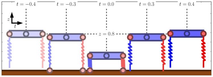
Figure 3: Illustration of a periodic orbit in the system depicted in Fig. 1(right) undergoing simultaneous activation (and, subsequently, simultaneous deactivation) of unilateral constraints. (top) Snapshots of the trajectory at apex ($t=\pm 0.4$), touchdown/liftoff ($t=\pm 0.3$), and nadir ($t=0.0$). (bottom) Illustration of Poincaré map $P:V\rightarrow S$ over the apex section $S$, defined in Sec. 6.2; trajectories initialized in the open subset $V\subset S$ return to $S$. The set $V$ is partitioned into regions where selection functions for the piecewise–$C^{r}$ map $P$ are active: initial conditions with $\theta>0$, where the left leg constraint activates before the right, are colored blue; initial conditions with $\theta<0$ are colored red. Along the trajectory generated by the fixed point $P(\rho,\dot{\rho})=(\rho,\dot{\rho})$ (colored black), simultaneous constraint activation is indicated by the trajectory passing through the intersection of the constraint surfaces for the right ($\left\{a_{r}=0\right\}$) and left ($\left\{a_{l}=0\right\}$) legs; similarly for simultaneous deactivation through the intersection $\left\{\lambda_{l}=0\right\}\cap\left\{\lambda_{r}=0\right\}$. A nearby trajectory initialized at $(p,\dot{p})\in V$ (colored blue) undergoes constraint activation and deactivation at distinct instants in time.

We start by constructing a Poincaré map for the periodic orbit $\phi^{(\rho,\dot{\rho})}$. Let $S\subset TQ$ be a Poincaré section for $\phi^{(\rho,\dot{\rho})}$ at $(\rho,\dot{\rho})$, i.e. a $C^{r}$ embedded codimension–1 submanifold containing $(\rho,\dot{\rho})$ that is transverse to the vector field in (1a). For a concrete example we refer to the model in Fig. 3 where $S$ is a Poincaré section about an apex height of $z~{}=~{}0.8$ and $\rho$ is a position vector with body height $z=0.8$, rotation $\theta=0$, and the legs oriented perpendicular to the body orientation. Given zero initial velocity, the time period is $T=0.8$.

Since $\phi$ is continuous by Lem. 2 (continuity across contact mode sequences), there exists a first–return time $\tau\colon V\rightarrow(0,\infty)$ defined over an open neighborhood $V\subset S$ containing $(\rho,\dot{\rho})$ such that $\phi(\tau(q,\dot{q}),(q,\dot{q}))\in S$ for all $(q,\dot{q})\in V$ and $\tau(\rho,\dot{\rho})=T$; we let $P:V\rightarrow S$ be the Poincaré (or first–return) map defined by

$$\forall(q,\dot{q})\in V\colon P(q,\dot{q})=\phi(\tau(q,\dot{q}),(q,\dot{q}))\in S.$$ (28)

As an illustration, $(p,\dot{p})\in V$ in Fig. 3(bottom) generates a trajectory initialized near $(\rho,\dot{\rho})$ that undergoes constraint activations and deactivations at distinct instants in time, activating the left leg constraint before activating the right leg constraint, then deactivating both constraints in the same order. Since $\phi$ is $PC^{r}$ and $S$ is a $C^{r}$ manifold we conclude that $\tau$ is $PC^{r}$ [5, Thm. 10], whence $P$ is $PC^{r}$. This implies in particular that its B–derivative $DP(\rho,\dot{\rho})$ provides a continuous and piecewise–linear first–order approximation for $P$. To assess exponential stability of $\phi^{(\rho,\dot{\rho})}$, it suffices to determine conditions under which the piecewise–linear map $DP(\rho,\dot{\rho})$ is exponentially contractive or expansive. This task is nontrivial since, as is well–known [3, Ex. 2.1], a piecewise–linear system constructed from stable subsystems may be unstable; similarly, a system constructed from unstable subsystems may be stable. We refer to [22, Sec. II-A] for a thorough review of state–of–the–art methods for assessing stability of piecewise–linear systems, and provide some example tests below.

Since $P$ is $PC^{r}$, there exists a finite collection $\left\{P_{\omega}\right\}_{\omega\in\Omega}$ of $C^{r}$ selection functions for $P$, and we assume the neighborhood $V$ was chosen sufficiently small that $P_{\omega}\colon V\rightarrow S$ for each $\omega\in\Omega$. Let $R_{\omega}\subset V$ denote the region where the selection function $p_{\omega}$ is active (i.e. where $P|_{R_{\omega}}=P_{\omega}|_{R_{\omega}}$). The first order approximation for $P_{\omega}$ is given by the classical (Jacobian/Fréchet) derivative $DP_{\omega}\colon TV\rightarrow TS$, which can be calculated using the (classical) chain rule. If there is a norm $\left\|\cdot\right\|:\mathbb{R}^{2d-1}\rightarrow\mathbb{R}$ with respect to which $DP_{\omega}(\rho,\dot{\rho})$ is a contraction for all $\omega\in\Omega$ (i.e. for all $\omega\in\Omega$ the induced norm $\left\|DP_{\omega}(\rho,\dot{\rho})\right\|<1$), then the periodic orbit $\phi^{(\rho,\dot{\rho})}$ is exponentially stable [5, Prop. 15]. (Note that it does not suffice to find a different norm $\|\cdot\|_{\omega}$ for each $\omega\in\Omega$ with respect to which $DP_{\omega}(\rho,\dot{\rho})$ is a contraction. [3, Ex. 2.1]). If instead for some $\omega\in\Omega$ there exists an eigenvector $\nu$ for $DP_{\omega}(\rho,\dot{\rho})$ with eigenvalue $\lambda$ such that $\left|\lambda\right|>1$ and both $\nu$ and $DP_{i}(\rho,\dot{\rho})\nu\in R_{i}$, then $(\rho,\dot{\rho})$ is exponentially unstable; this instability test is illustrated in Fig. 4.

Figure 4: A Poincaré section $S$ (outer grey box) and the neighborhood $V$ (inner circle) containing $(\rho,\dot{\rho})$ over which the piecewise–differentiable Poincaré (or first–return) map $P:V\rightarrow S$ is defined. In this example, the color corresponds to one of the two selection functions and the shaded region of $V$ denoting the active selection function for a perturbation in the given direction. $B$ is the unit ball. The dotted ellipses are the unit ball transformed by the respective selection functions with the arrow indicating the principle axes. (left) The Poincaré map $P$ corresponds to an unstable system. One of the eigenvectors $\nu_{1}$ maps a unit vector outside the unit ball. Additionally, the selection function for which $\nu_{1}$ is an eigenvector for is active for any perturbation lying along $\nu_{1}$. (right) The given instability check is not able to determine if the Poincaré map $P$ is unstable due to the lack of active eigenvectors mapping a unit vector outside the unit ball. The active selection function for a perturbation along $\nu_{2}$ is not the selection function for which $\nu_{2}$ is an eigenvector for.

6.3 Assessing controllability

In this section we consider the problem of assessing (small–time, local [33]) controllability along a trajectory in a mechanical system subject to unilateral constraints. The local control problem has been solved quite satisfactorily along trajectories in such systems that undergo constraint activation and deactivation at distinct instants in time for cases where the control input influences the discrete–time [23] or continuous–time [27] portions of (1). We concern ourselves here with the controlled dynamics in (27), and focus our attention on trajectories that activate and/or deactivate multiple constraints simultaneously since (to the best of our knowledge) this case has not previously been addressed in the literature.

Toward that end, let $\widetilde{\phi}:\widetilde{\mathscr{F}}\rightarrow TA$ be the flow of (27) (a mechanical system subject to unilateral constraints with input parameter $u\in U=\mathbb{R}^{m}$), and let $\widetilde{\phi}^{((\rho,\dot{\rho}),\mu)}$ be a trajectory initialized at $(\rho,\dot{\rho})\in TA$ with input parameter $\mu\in U$. If $\widetilde{\phi}$ were $C^{1}$ at $(t,(\rho,\dot{\rho}),\mu)\in\widetilde{\mathscr{F}}$, then (small–time) local controllability about $\widetilde{\phi}^{((\rho,\dot{\rho}),\mu)}$ could be determined using an invertibility condition on the (Jacobian) matrix $D\widetilde{\phi}(t,(\rho,\dot{\rho}),\mu)$. Indeed, a straightforward application of the Implicit Function Theorem [19, Thm. C.40] shows that if the subblock $D_{U}\widetilde{\phi}(t,(\rho,\dot{\rho}),\mu)$, which transforms first–order variations in the input parameter $u$ into the resulting first–order variations in the state $(q,\dot{q})$ at time $t$, is invertible, then (27) is (small–time) locally controllable along $\widetilde{\phi}^{((\rho,\dot{\rho}),\mu)}$ [20, Thm. 8].

In contrast to the preceding discussion, suppose now that $\widetilde{\phi}^{((\rho,\dot{\rho}),\mu)}$ undergoes simultaneous constraint activations in the time interval $(0,t)\subset[0,\infty)$. In this case $\widetilde{\phi}$ will not be $C^{1}$ at $(t,(\rho,\dot{\rho}),\mu)$, so the classical test for controllability is not applicable. If all constraint activations and deactivations are admissible for $\widetilde{\phi}^{((\rho,\dot{\rho}),\mu)}$ and nearby trajectories, then Thm. 1 (piecewise differentiability across contact mode sequences) implies that $\widetilde{\phi}$ is $PC^{r}$ at $(t,(\rho,\dot{\rho}),\mu)$ and hence possesses a B–derivative $D\widetilde{\phi}(t,(\rho,\dot{\rho}),\mu)$, that is, a continuous and piecewise–linear first–order approximation. By analogy with the classical test [20, Thm. 8], a variant of the Implicit Function Theorem applicable to $PC^{r}$ functions [31, Thm. 4.2.3] can be used to derive a sufficient condition for small–time local controllability along $\widetilde{\phi}^{((\rho,\dot{\rho}),\mu)}$: if the piecewise–linear function that transforms first–order variations in (an appropriately–chosen subspace of) input parameters $u$ into the resulting first–order variations in the state $(q,\dot{q})$ at time $t$ is a (piecewise–linear) homeomorphism, then (27) is (small–time) locally controllable along $\widetilde{\phi}^{((\rho,\dot{\rho}),\mu)}$.

References

- [1] M. A. Aizerman and F. R. Gantmacher “Determination of Stability by Linear Approximation of a Periodic Solution of a System of Differential Equations with Discontinuous Right–Hand Sides” In The Quarterly Journal of Mechanics and Applied Mathematics 11.4 Oxford University Press, 1958, pp. 385–398 DOI: 10.1093/qjmam/11.4.385
- [2] Patrick Ballard “The Dynamics of Discrete Mechanical Systems with Perfect Unilateral Constraints” In Archive for Rational Mechanics and Analysis 154.3 Springer-Verlag, 2000, pp. 199–274 DOI: 10.1007/s002050000105
- [3] M. S. Branicky “Multiple Lyapunov functions and other analysis tools for switched and hybrid systems” In IEEE Transactions on Automatic Control 43.4, 1998, pp. 475–482 DOI: 10.1109/9.664150
- [4] Samuel A. Burden “A Hybrid Dynamical Systems Theory for Legged Locomotion”, 2014 URL: http://www.eecs.berkeley.edu/Pubs/TechRpts/2014/EECS-2014-167.html
- [5] Samuel A. Burden, S. Shankar Sastry, Daniel E. Koditschek and Shai Revzen “Event–Selected Vector Field Discontinuities Yield Piecewise–Differentiable Flows” In SIAM Journal on Applied Dynamical Systems 15.2, 2016, pp. 1227–1267 DOI: 10.1137/15M1016588
- [6] Samuel A. Burden, Humberto Gonzalez, Ramanarayan Vasudevan, Ruzena Bajcsy and S. Shankar Sastry “Metrization and Simulation of Controlled Hybrid Systems” In IEEE Transactions on Automatic Control 60.9, 2015, pp. 2307–2320 DOI: 10.1109/TAC.2015.2404231
- [7] Samuel A. Burden, Shai Revzen and S. Shankar Sastry “Model Reduction Near Periodic Orbits of Hybrid Dynamical Systems” In IEEE Transactions on Automatic Control 60.10, 2015, pp. 2626–2639 DOI: 10.1109/TAC.2015.2411971
- [8] M. Di Bernardo, C. J. Budd, P. Kowalczyk and A. R. Champneys “Piecewise–smooth dynamical systems: theory and applications” Springer, 2008
- [9] A. F. Filippov “Differential equations with discontinuous righthand sides” Springer, 1988
- [10] J. W. Grizzle, G. Abba and F. Plestan “Asymptotically stable walking for biped robots: Analysis via systems with impulse effects” In IEEE Transactions on Automatic Control 46.1, 2002, pp. 51–64 DOI: 10.1109/9.898695
- [11] J. Guckenheimer and P. Holmes “Nonlinear oscillations, dynamical systems, and bifurcations of vector fields” Springer, 1983
- [12] N. Hinrichs, M. Oestreich and K. Popp “Dynamics of oscillators with impact and friction” In Chaos, Solitons & Fractals 8.4 Elsevier, 1997, pp. 535–558
- [13] I. A. Hiskens and M. A. Pai “Trajectory sensitivity analysis of hybrid systems” In IEEE Transactions on Circuits and Systems I: Fundamental Theory and Applications 47.2, 2000, pp. 204–220 DOI: 10.1109/81.828574
- [14] Yildirim Hürmüzlü and D. B. Marghitu “Rigid Body Collisions of Planar Kinematic Chains With Multiple Contact Points” In The International Journal of Robotics Research 13.1 Sage Publications, 1994, pp. 82–92 DOI: 10.1177/027836499401300106
- [15] Aaron M. Johnson, Samuel A. Burden and Daniel E. Koditschek “A Hybrid Systems Model for Simple Manipulation and Self–Manipulation Systems” In The International Journal of Robotics Research 35.11, 2016, pp. 1289–1327 DOI: 10.1177/0278364916639380
- [16] Krzysztof C Kiwiel “Methods of descent for nondifferentiable optimization” Springer, 1985
- [17] Scott Kuindersma, Robin Deits, Maurice Fallon, Andrés Valenzuela, Hongkai Dai, Frank Permenter, Twan Koolen, Pat Marion and Russ Tedrake “Optimization–based locomotion planning, estimation, and control design for the atlas humanoid robot” In Autonomous Robots, 2015, pp. 1–27 DOI: 10.1007/s10514-015-9479-3
- [18] V. Kumar, E. Todorov and S. Levine “Optimal control with learned local models: Application to dexterous manipulation” In IEEE International Conference on Robotics and Automation (ICRA), 2016, pp. 378–383 DOI: 10.1109/ICRA.2016.7487156
- [19] J. M. Lee “Introduction to smooth manifolds” Springer–Verlag, 2012
- [20] A. U. Levin and K. S. Narendra “Control of nonlinear dynamical systems using neural networks: controllability and stabilization” In IEEE Transactions on Neural Networks 4.2, 1993, pp. 192–206 DOI: 10.1109/72.207608
- [21] Sergey Levine, Chelsea Finn, Trevor Darrell and Pieter Abbeel “End–to–end Training of Deep Visuomotor Policies” In Journal of Machine Learning Research 17.1 JMLR.org, 2016, pp. 1334–1373 URL: http://dl.acm.org/citation.cfm?id=2946645.2946684
- [22] Hai Lin and P. J. Antsaklis “Stability and Stabilizability of Switched Linear Systems: A Survey of Recent Results” In IEEE Transactions on Automatic Control 54.2, 2009, pp. 308–322 DOI: 10.1109/TAC.2008.2012009
- [23] A.W. Long, T.D. Murphey and K.M. Lynch “Optimal motion planning for a class of hybrid dynamical systems with impacts” In IEEE International Conference on Robotics and Automation, 2011, pp. 4220–4226 DOI: 10.1109/ICRA.2011.5980154
- [24] Katja D. Mombaur, Richard W. Longman, Hans Georg Bock and Johannes P. Schlöder “Open–loop Stable Running” In Robotica 23.1 New York, NY, USA: Cambridge University Press, 2005, pp. 21–33 DOI: 10.1017/S026357470400058X
- [25] Y. Or and A. D. Ames “Stability and Completion of Zeno Equilibria in Lagrangian Hybrid Systems” In IEEE Transactions on Automatic Control 56.6, 2011, pp. 1322–1336 DOI: 10.1109/TAC.2010.2080790
- [26] C. D. Remy, K. Buffinton and R. Siegwart “Stability Analysis of Passive Dynamic Walking of Quadrupeds” In The International Journal of Robotics Research 29.9 Sage Publications, 2010, pp. 1173–1185 DOI: 10.1177/0278364909344635
- [27] M. Rijnen, A. Saccon and H. Nijmeijer “On optimal trajectory tracking for mechanical systems with unilateral constraints” In IEEE Conference on Decision and Control, 2015, pp. 2561–2566 DOI: 10.1109/CDC.2015.7402602
- [28] Stephen M. Robinson “Local structure of feasible sets in nonlinear programming, Part III: Stability and sensitivity” In Nonlinear Analysis and Optimization 30, Mathematical Programming Studies Springer Berlin Heidelberg, 1987, pp. 45–66 DOI: 10.1007/BFb0121154
- [29] R.T. Rockafellar “A Property of Piecewise Smooth Functions” In Computational Optimization and Applications 25.1/3 Springer-Verlag, 2003, pp. 247–250 DOI: 10.1023/A:1022921624832
- [30] M. Schatzman “Uniqueness and continuous dependence on data for one–dimensional impact problems” In Mathematical and Computer Modelling 28.4—8, 1998, pp. 1–18 DOI: 10.1016/S0895-7177(98)00104-6
- [31] Stefan Scholtes “Introduction to piecewise differentiable equations” Springer–Verlag, 2012 DOI: 10.1007/978-1-4614-4340-7
- [32] David E. Stewart “Rigid–Body Dynamics with Friction and Impact” In SIAM Review 42.1 Philadelphia, PA, USA: Society for IndustrialApplied Mathematics, 2000, pp. 3–39 DOI: 10.1137/S0036144599360110
- [33] H. J. Sussmann “A General Theorem on Local Controllability” In SIAM Journal on Control and Optimization 25, 1987, pp. 158–194
- [34] E. D. Wendel and A. D. Ames “Rank deficiency and superstability of hybrid systems” In Nonlinear Analysis: Hybrid Systems 6.2, 2012, pp. 787–805 DOI: 10.1016/j.nahs.2011.09.002