Topological order and equilibrium in a condensate of exciton-polaritons

We report the observation of the Berezinskii–Kosterlitz–Thouless transition for a 2D gas of exciton-polaritons, and through the joint measurement of the first-order coherence both in space and time we bring compelling evidence of a thermodynamic equilibrium phase transition in an otherwise open driven/dissipative system. This is made possible thanks to long polariton lifetimes in high-quality samples with small disorder and in a reservoir-free region far away from the excitation spot, that allow topological ordering to prevail. The observed quasi-ordered phase, characteristic for an equilibrium 2D bosonic gas, with a decay of coherence in both spatial and temporal domains with the same algebraic exponent, is reproduced with numerical solutions of stochastic dynamics, proving that the mechanism of pairing of the topological defects (vortices) is responsible for the transition to the algebraic order. Finally, measurements in the weak-coupling regime confirm that polariton condensates are fundamentally different from photon lasers and constitute genuine quantum degenerate macroscopic states.

Collective phenomena which involve the emergence of an ordered phase in many-body systems have a tremendous relevance in almost all fields of knowledge, spanning from physics to biology and social dynamics ^{1; 2}. While the physical mechanisms can be very different depending on the system considered, statistical mechanics aims at providing universal descriptions of phase transitions on the basis of few and general parameters, the most important being dimensionality and symmetry ^{3; 4; 5}. The spontaneous symmetry breaking of Bose–Einstein condensates (BEC) below a critical temperature $T>0$ is a remarkable example of such a transition, with the emergence of an extended coherence giving rise to a long range order (LRO) ^{6; 7; 8}. Notably, in infinite systems with dimensionality $d\leq 2$, true LRO cannot be established at any finite temperature ⁹. This is fundamentally due to the presence of low-energy long-wavelength thermal fluctuations (i.e. Goldstone modes) that prevail in $d\leq 2$ geometries.

However, if we accept a lower degree of order, characterised by an algebraic decay of coherence, it is still possible to make a clear distinction between such a quasi-long-range-ordered (QLRO) and a disordered phase in which the coherence is lost in a much faster, exponential way. Such transition, in two dimensions (2D) and at a critical temperature $T>0$, is explained in the Berezinskii–Kosterlitz–Thouless theory (BKT) by the proliferation of vortices—the fundamental topological defects—of opposite signs ¹⁰. This theory is well established for 2D ensembles of cold atoms in thermodynamic equilibrium, where the transition is linked to the appearance of a linear relationship between the energy and the wavevector of the excitations in the quasi-ordered state ¹¹. The joint observation of spatial and temporal decay of coherence has never been observed in atomic systems, mainly because of technical difficulties in measuring long-time correlations. These are important observables to bring together because an algebraic decay, with the same exponent $\alpha$, for both the temporal and spatial correlations of the condensed state, implies a linear dispersion for the elementary excitations^{12; 13; 14}.

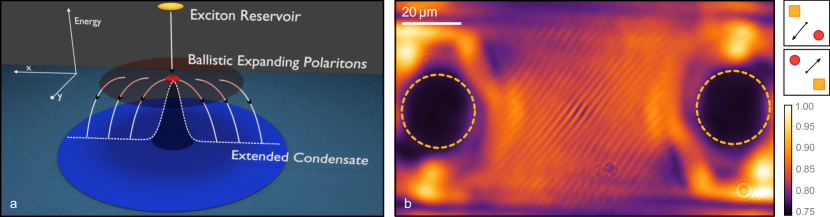
Figure 1: Sketch of the pumping mechanism and interferogram. a, Spatial cross section (x,y) at different energies, where the vertical axes represents increasing energies. The carriers, injected by the pumping laser, relax quickly into excitonic states (yellow area) spatially confined within the pumping spot region. Efficient scattering from the exciton reservoir into polariton states results in a region of high polariton density (red area) which expands radially outwards and relax into lower energy states. Above a threshold power, an extended 2D polariton condensate (blue area) is formed outside of the pumped region. b, Interference pattern of the extended 2D polariton condensate, obtained rotating one arm of the interferometer as the symbols on the right. The circles in yellow, dashed line indicate the blue-shifted region (emission is filtered around k=0) corresponding to the position of the laser spot.

On the other hand, semiconductor systems such as microcavity polaritons (dressed photons with sizeable interactions mediated by the excitonic component) since the report of their condensation¹⁵ appear to be ideal platforms to extend the investigation of many-body physics to the more general scenario of phase transitions in driven-dissipative systems ¹⁶. However, establishing if the transition can actually be governed by the same BKT process as for equilibrium system has proven to be challenging from both the theoretical^{17; 18; 19} and experimental perspective. Indeed, the dynamics of phase fluctuations is strongly modified by pumping and dissipation, and the direct measurement of their dispersion by photoluminescence and four-wave-mixing experiments is limited by the short polariton lifetime, by the pumping-induced noise and by the low resolution close to condensate energy^{20; 21; 22}. Moreover, the algebraic decay of coherence has been experimentally demonstrated only in spatial correlations, while only exponential or Gaussian decays of temporal coherence, which are not compatible with a BKT transition, have been reported until now^{23; 24; 25; 26}. In particular, the lack of a power law decay of temporal correlations is a strong argument against a true BKT transition, as will be demonstrated later on in a straightforward counter-example of a strongly out-of-equilibrium polariton system. For this reason, it has been a matter of constant debate in the field what is the nature of the various polariton phases, what are the observables that allow to determine a QLRO, if any, and how they compare with equilibrium 2D condensates and with lasers ^{27; 28; 29; 30; 31; 32}. Recently, thanks to a new generation of samples with record polariton lifetimes, a thermalization across the condensation threshold has been reported via constrained fitting to Bose–Einstein distribution, suggesting a weaker effect of dissipation in these systems ³³. However, to unravel the mechanisms that drive the transition, and characterize its departure from the equlibrium condition, it is crucial to measure the correlations between distant points in space and time as we move from the disordered to the quasi-ordered regime^{13; 14; 34; 35}. So far, all attempts in this direction have been thwarted, not only by the polariton lifetime being much shorter than the thermalization time, but also by sample inhomogeneities ^{36; 37} and/or small extents of the condensate. The latter, in particular, limits the power-law decay of the spatial coherence to the small spatial extension of the exciton reservoir set by the excitation spot ^{38; 39; 23}, which could result in an effective trapping mechanism ⁴⁰ and finite size effects ²⁸.

In this work, using a high quality sample (in terms of long lifetimes and spatial homogeneity) to form and control a reservoir-free condensate of polaritons over a largely extending spatial region, we make the first observation (in any system) of the transition to a QLRO phase both in spatial and in temporal domains. Remarkably, the convergence of spatial and temporal decay of coherence allows us to identify the connection with the classic equilibrium BKT scenario, in which for systems with linear spectrum the exponents take exactly the same value $\alpha\leq 1/4$.¹⁴ Stochastic simulations tuned to the experimental conditions, that reproduce the experimental observations in both space and time, further allow us to track vortices in each realisation of the condensate, confirming the topological origin of the transition. All these results settle the BKT nature of the 2D phase-transition for driven/dissipative polaritons in high quality samples, providing the equilibrium limit that allows to develop the paradigm of non-equilibrium regimes. Finally, this proves that a quasi-ordered polariton state is fundamentally different from a laser—excitons in a cavity under weak coupling conditions—for which a power-law decay of the first order coherence is observed only in space but not in time correlations, also putting to rest the long-time debate whether polaritons above threshold are distinct from a laser, and can indeed be called a condensate^{41; 42}.

Results

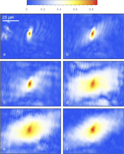
Figure 2: Two dimensional first order correlation function $g^{(1)}(\mathbf{r})$ at different densities. From the top left corner, d=$0.015\text{\,}\mathrm{p}\mathrm{o}\mathrm{l}\mathrm{/}\mathrm{\SIUnitSymbolMicro}\mathrm{m}\mathrm{{}^{2}}$, d=$0.1\text{\,}\mathrm{p}\mathrm{o}\mathrm{l}\mathrm{/}\mathrm{\SIUnitSymbolMicro}\mathrm{m}\mathrm{{}^{2}}$, d=$0.15\text{\,}\mathrm{p}\mathrm{o}\mathrm{l}\mathrm{/}\mathrm{\SIUnitSymbolMicro}\mathrm{m}\mathrm{{}^{2}}$, d=$0.4\text{\,}\mathrm{p}\mathrm{o}\mathrm{l}\mathrm{/}\mathrm{\SIUnitSymbolMicro}\mathrm{m}\mathrm{{}^{2}}$, d=$0.9\text{\,}\mathrm{p}\mathrm{o}\mathrm{l}\mathrm{/}\mathrm{\SIUnitSymbolMicro}\mathrm{m}\mathrm{{}^{2}}$, d=$1.2\text{\,}\mathrm{p}\mathrm{o}\mathrm{l}\mathrm{/}\mathrm{\SIUnitSymbolMicro}\mathrm{m}\mathrm{{}^{2}}$ in a, b, c, d, e, f, respectively.

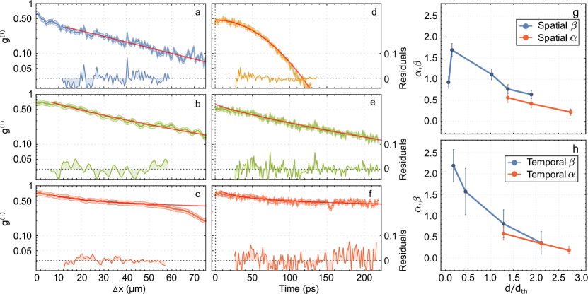
Figure 3: Coherence decay and BKT phase transition. a, b, c, Details for $\Delta x>0$ of the exponential (blue data), stretched exponential (green data), power law (red data) spatial decay of $g^{(1)}(x,-x)$ and corresponding fitting residuals. d, e, f, $g^{(1)}(t,t+\Delta t)$ for $\Delta t>0$ of the Gaussian (yellow data), stretched exponential (green data), power law (red data) temporal decay and corresponding fitting residuals. g, Blue line: $\beta$ exponent from the stretched exponential fitting of $g^{(1)}(x,-x)$ as a function of polariton densities. Red line: $\alpha$ exponent from the power law fitting of $g^{(1)}(x,-x)$ in the above threshold density range. h, Blue line: $\beta$ exponent from the stretched exponential fitting of $g^{(1)}(t,t+\Delta t)$ as a function of polariton densities. Red line: $\alpha$ exponent from the power law fitting of $g^{(1)}(t,t+\Delta t)$ in the above threshold density range. Error bars from fitting parameters errors.

The sample is excited non-resonantly (Methods), leading to the formation of the exciton reservoir (yellow region in Fig. 1a) which is localised within the pumping spot area due to the low exciton mobility. In turn, the repulsive interactions between excitons induce the energy blueshift of the polariton resonance at the center of the pumping spot (the dashed-white line in Fig. 1a is the energy blueshift in the $x$ direction, corresponding to the Gaussian intensity profile of the exciting beam). Polaritons, which are formed beneath the exciton reservoir through energy relaxation, are much lighter particles than excitons and are accelerated outwards from the center of the spot. As sketched in Fig. 1a, the cloud of expanding polaritons propagates ballistically for tens of microns, before eventually relaxing into the lowest energy level outside of the blue-shifted region. This process of expansion and relaxation leads, above a critical density, to the formation of a condensed state at the bottom of the lower polariton branch, which extends over a wide spatial region and even at long distances from the position of the pumping spot ⁴³. The light emitted by the sample carries all the information about the spatio-temporal correlations of the extended polariton condensate, that can be measured by a Michelson interferometer as described in the following and in the Supplementary Information.

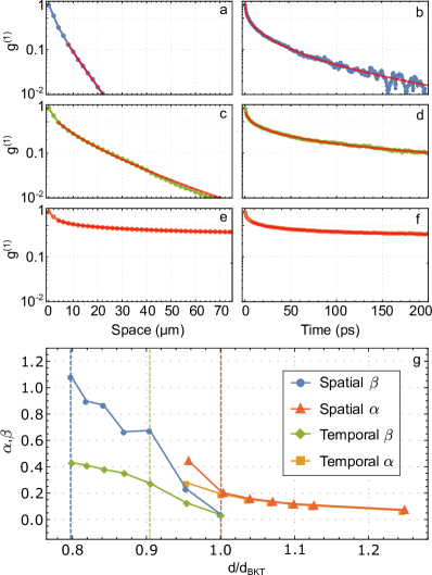
Figure 4: Decay of coherence from stochastic analysis. a,c,e Spatial decay of coherence. Respectively, an exponential decay, a stretched exponential with $\beta=0.67$ and a power law decay with $\alpha=0.20$. b,d,f, Temporal decay of coherence. Respectively, a stretched exponential with $\beta=0.41$, a stretched exponential with $\beta=0.27$ and a power law with $\alpha=0.20$. These three cases are indicated in g with blue, green and red vertical dashed lines. g, Exponents $\beta$ of the stretched exponential fit, for spatial (blue) and temporal (green). Exponents $\alpha$ of the power law fitting for spatial (red) and temporal (orange). Note, we normalise the density $d$ to the density $d_{\rm BKT}$ at which the algebraic decay clearly fits the data better then the stretched exponential (see Fig. 6 in SI).

The spatial correlation is extracted from the interference pattern obtained overlapping the 2D emission map with its centro-symmetric image. In Fig. 1b, the interference fringes are visible around the center of the image, which is the autocorrelation point $\mathbf{r}=\mathbf{r_{0}}$. The phase coherence in space is therefore measured by the first order correlation function $g^{(1)}(\mathbf{r}-\mathbf{r_{0}})$ (where omitted, $\mathbf{r_{0}}=0$ and $t=t^{\prime}$ is assumed). In Fig. 2, $g^{(1)}(\mathbf{r})$ is shown in colour-scale for different values of the polariton density. Increasing the pumping power, a higher level of coherence is sustained over larger distances (Fig. 2(a-e)), up to a maximum in Fig. 2e. Note that the high quality of the sample allows a uniform coherence to extend over a wide spatial region of about $80\text{\,}\mathrm{\SIUnitSymbolMicro m}$$\times$$60\text{\,}\mathrm{\SIUnitSymbolMicro m}$. Increasing further the excitation power results in the shrinking of the spatial extension of the coherence, as shown in Fig. 2f.

In Fig. 3, the horizontal line profile $|g^{(1)}(x,-x)|$ passing through $\mathbf{r_{0}}$, for $\Delta x>0$ (with $\Delta x\equiv 2x$), is studied at increasing pumping powers (Fig. 3(a-c)). To allow a uniform description across the transition, both a power law and a stretched exponential functions are used in the fitting procedure:

$$|g^{(1)}(x,-x)| =A|2x|^{-\alpha}$$ (1)

$$|g^{(1)}(x,-x)| =Ae^{-B|2x|^{\beta}}$$ (2)

with $B$ a scale parameter for the $x$-axis. At low pumping power (Fig. 3a), the decay is exponential and it is well fitted by eq. (2) with $\beta\approx 1$. Increasing the pumping power, the exponential decay first changes into a short range envelope $\beta>1$, and then, at the threshold density $\text{d}_{\text{th}}$ for the nonlinear increase of the ground-state population ⁴³, coherence starts to build up at larger distances. This corresponds to a change in the slope of the decay, which is still best fitted by eq. (2), but now with $\beta<1$ (Fig. 3b). Finally, at $d\approx 2.7\leavevmode\nobreak\ \text{d}_{\text{th}}$, a power law decay is evident (Fig. 3c), with a high degree of spatial coherence (>$50\text{\,}\%$) extending over distances of $\approx$50\text{\,}\mathrm{\SIUnitSymbolMicro m}$$. Remarkably, this slow decay is characterized by the exponent $\alpha=0.22$. In Fig. 3g, the $\alpha$ and $\beta$ exponents are shown at different densities: while below threshold only eq. (2) is able to fit the experimental data, above threshold the best fit is given by eq. (1) (see Supplementary Information). However, as will be shown in the following, it is essential to verify that a similar behavior is also observed for the temporal correlations.

The decay of temporal coherence is extracted by using the long delay line to change the relative temporal delay of the two interferometer arms up to $200$ ps (see Methods and Supplementary Information). In Fig. 3(d-f), the temporal coherence at the autocorrelation point $g^{(1)}(t,t+\Delta t)$ is shown for three different polariton densities. In Fig. 3h, the $\alpha$ and $\beta$ exponents of equations (1) and (2) that best fit the experimental data are shown across the transition. Below threshold, coherence decays quickly and follows a Gaussian slope ($\beta\approx 2$). At $d=1.3\leavevmode\nobreak\ \text{d}_{\text{th}}$, the temporal coherence can be best fitted by (2) with an exponent $\beta\approx 0.8$ (or, with a slightly worst fit, with a power-law of exponent $\alpha\approx 0.57$), while at $d\approx 2.7\leavevmode\nobreak\ \text{d}_{\text{th}}$, the long time behaviour clearly follows a power law with $\alpha=0.2$. The residuals analysis proves the agreement between the experimental data and the fitting model (see Supplementary Information). Crucially, also for time correlations, $\alpha<0.25$, which coincides, within the experimental accuracy, with the one obtained from the spatial coherence at the corresponding density.

We performed complementary theoretical analysis, based on the exact solution of the stochastic equations of motions ¹⁹ (see Methods), with the same microscopic parameters as the ones of the experiment. We observed the same crossover from an exponential via stretched exponential to an algebraic decay of coherence in space and time (Fig. 4). In particular, for our long polariton lifetime, we see the spatial and temporal $\alpha$ being the same and always smaller then 1/4 above the BKT threshold (Fig. 4g), showing that the drive and dissipation do not prevail in this good quality sample in contrast to the earlier studied non-equilibrium cases ^{19; 23}.

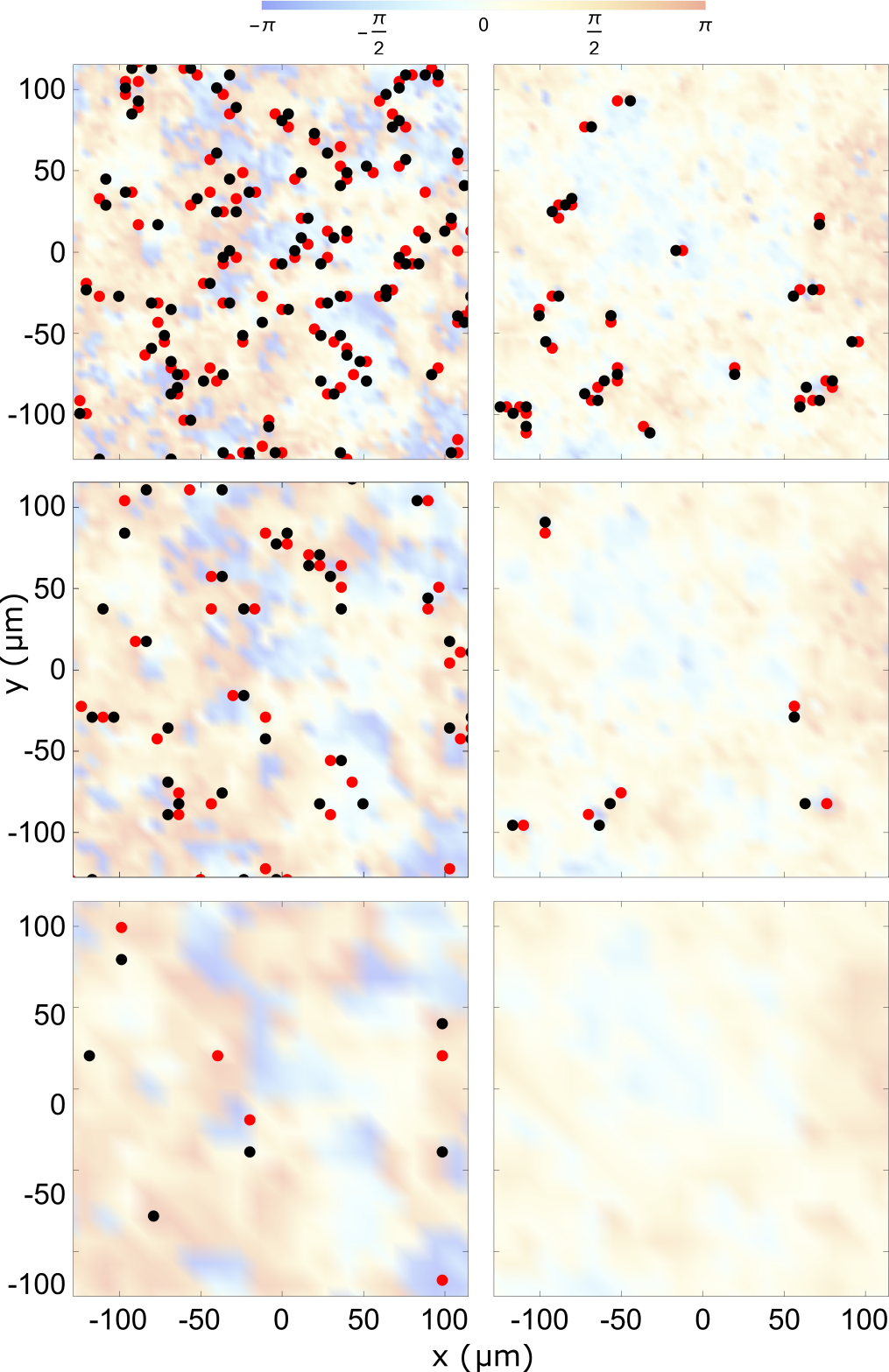
Figure 5: Vortex-antivortex distribution map. Top, Vortices (V) in red and anti-vortices (AV) in black just before (left) and after (right) the BKT transition with parameters as in Fig. 4c and e, respectively. Middle-Bottom The same as in Top but after filtering off in two steps high momentum states to eliminate bound pairs. Such filtering reveals the presence of free vortices. Note that there are no free vortices when spatial and temporal coherence show algebraic decay (right) but there are some free vortices in the case of stretched exponential decay of coherence (left). The underlying colour map shows the phase profile of the field.

Additionally, while the vortex-antivortex binding cannot be directly observed in the experiments, which average over many realizations, the numerical analysis is able to track the presence of free vortices in each single realisation, confirming the topological origin of the transition. Indeed, we see clearly that, in the algebraically ordered state, free vortices do not survive and the pairing is complete (Fig. 5 right). In contrast, the exponential and stretched-exponential regimes both show the presence of free vortices (Fig. 5 left), the number of which decreases as we move across the transition. Since the stretched exponential phase is always associated with some presence of free vortices, this supports that we are observing a BKT crossover rather than a Kardar-Parisi-Zhang phase ¹⁷.

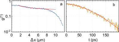
Figure 6: Spatial and temporal coherence in weak coupling regime. a, Spatial coherence showing a power law decay with $\alpha=0.253$. b, Temporal decay of coherence with stretched exponential fitting exponent $\beta=1.8$.

Finally, to highlight the importance of studying correlation not only in the space but also in the temporal domain, we used a microcavity in the weak-coupling regime, showing that a power law decay of coherence in space is associated in this case to a Gaussian decay in time. Using a sample with a lower quality factor and less quantum wells, we induce, under high non-resonant pumping, the photon-laser regime (as in a VCSEL) ^{44; 45}. Despite the fact that this system is clearly out-of-equilibrium, it shows a power law decay of spatial coherence with $\alpha=0.25$ (Fig. 6a) within the pumping spot region (with a radius of about $10\text{\,}\mathrm{\SIUnitSymbolMicro m}$). Remarkably, the behavior of spatial correlations is very similar to what obtained in Ref[23], but the temporal coherence, shown in Fig. 6b, follows a quasi-Gaussian decay (stretched exponential with $\beta$ exponent about 1.8), not compatible with the algebraic order characteristic of the BKT phase. This shows that a consistent behavior between time and space is necessary to evidence the BKT transition in driven/dissipative systems.

Conclusions

In conclusion, we observed the formation of an ordered phase in two-dimensional driven/dissipative ensemble of bosonic quasiparticles, exciton-polaritons in semiconductor microcavities, exploring both spatial and temporal correlations across the transition. This system lies at the interface between equilibrium and out-of-equilibrium phase transitions, and it has been often compared both to Bose-Einstein condensates and to photon lasers. We show that the measurement of spatial correlations $g^{(1)}(\mathbf{r})$ alone is not sufficient to establish whether an open/dissipative system is at equilibrium. Instead, two distinct measurements, one in time and one in space domain, are needed. Satisfying this requirement, we report a power-law decay of coherence with the onset of the algebraic order at the same relative density and comparable exponents for both space and time correlations. We should stress that the exceptionally long polariton lifetime in the present sample allows us to reach the BKT phase transition at lower densities, and in the region without the excitonic reservoir, resulting in a lower level of dephasing. In our experiments, the absence of any trapping mechanism, be it from the exciton reservoir or potential minima, allows us to avoid the influence of finite-size effects in the temporal dynamics of the autocorrelation ¹⁴. Simulations with stochastic equations match perfectly the experimental results and demonstrate that the underlying mechanism of the transition is of the BKT type i.e. a topological ordering of free vortices into bound pairs, resulting in the coherence built up both in space and time. All these observations validate that polaritons undergo phase-transitions following the standard BKT picture, and fulfill the expected conditions of thermal equilibrium despite their driven/dissipative nature. Now that the equilibrium character of polaritons becomes a tunable parameter, the study of driven/dissipative phase transitions and of the universal scaling laws is within reach in this solid state device.

Methods

In the present experiment, polaritons were created in a planar semiconductor microcavity. The sample is described in detail in Ref.[43] and in the Supplementary Information. Polaritons are injected in the system by making use of a single-mode Ti:sapphire ring laser in continuous wave (CW) operation and tuned at energy around $1686.80\text{\,}\mathrm{meV}$ with a stabilized output wavelength and power (M2Squared SolsTis) to reduce fluctuations in the exciton reservoir. In particular, the energy of the laser is chosen to coincide with a minimum of the reflection stop band. To avoid sample thermal heating the pump laser is chopped at a frequency of $4$ kHz with a duty cycle of $8\%$. The chopper window aperture time (in the scale of $\mathrm{\SIUnitSymbolMicro s}$) is significantly larger than the polariton lifetime so it does not affect the dynamics. The excitation laser beam is focused in a Gaussian spot with a FWHM $\approx$ $20\text{\,}\mathrm{\SIUnitSymbolMicro m}$. The Gaussian laser profile in space is the best one to trigger the expulsion-relaxation mechanism, allowing the creation of a sufficiently uniform and extended polariton condensate. On the detection line, the emission from the sample is collected in epilayer configuration and it is sent to a Michelson interferometer with two delay lines as showed in Fig. S1 of SI. On the first interferometer arm, a short (fraction of the wavelength) piezo stage motorized is used to move a mirror. This allows the reconstruction of the spatial coherence $g^{(1)}(\mathbf{r}-\mathbf{r_{0}})$ using the sinusoidal envelope of the intensity (see Supplementary Fig. S2). On the second arm, a long (about $200$ ps) motorized screw actuator is used to change the position of the back-reflector to characterize the behavior of the coherence in time. By using the back-reflector, one of the two arms is centrosymmetrically rotated respect to the other and these two beams interfere on the focal plane of a CCD (Charge-Coupled Device) camera. To obtain energy resolved spatial and momentum emission images, a spectrometer is placed before the CCD detector.

References

Author contributions

D.C. and D.B. took and analysed the data. G.D. and M.H.S. performed stochastical numerical simulations. C.S.M. and F.P.L. discussed the results. D.C.,D.B, C.S.M., M.D.G., L.D., G.G, F.P.L. M.H.S. and D.S. co-wrote the manuscript. K.W. and L.N.P. fabricated the sample. D.S. coordinated and supervised all the work.

Topological order and equilibrium in a condensate of exciton-polaritons
Supplemental Material

Sample and experimental setup

The sample used in this work is a high quality factor (Q>100000) $\rm GaAs$/$\rm AlGaAs$ planar microcavity containing 12 $\rm GaAs$ quantum wells of 7 nm width, grouped in 3 blocks placed at the antinode positions of the electric field inside the cavity, with a collective Rabi splitting of $\hbar\Omega=$16\text{\,}\mathrm{meV}$$. The front (back) mirror consists of 34 (40) pairs of $\rm AlAs$/$\rm Al_{0.2}Ga_{0.8}As$ layers, with a polariton lifetime of about 100 ps ¹. The cavity detuning $\delta=\hbar(\rm\omega_{c}-\rm\omega_{x})$ is slightly negative ($\delta=$-1\text{\,}\mathrm{meV}$$), with the exciton energy $\rm\hbar\omega_{x}$=$1611.2\text{\,}\mathrm{meV}$. The sample is placed in a cryostat and kept at a temperature of about 10 K.

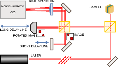
Figure S1: Michelson interferometer with two different delay lines: a first short one to measure the spatial decay of the correlation and a long one to evaluate the temporal decay.

The coherence properties are investigated using a Michelson interferometer with two different delay lines, as showed in Fig. S1.

First-order Correlation Function Decay

The first order correlation function is defined as:

$$g^{(1)}(r_{1},t_{1};r_{2},t_{2})=\frac{\langle\psi^{*}_{1}\psi_{2}\rangle}{\sqrt{\langle\psi^{*}_{1}\psi_{1}\rangle\langle\psi^{*}_{2}\psi_{2}\rangle}}$$ (S1)

with $\psi^{*}_{i}$ and $\psi_{i}$ the creation and annihilation operators for the space-time point $(r_{i},t_{i})$, with $i=1,2$. By changing the length of one path through the use of a motorized piezo stage, the relative phase is changed, and the intensity of each point of the image shows a sinusoidal envelope as shown in Fig. S2.

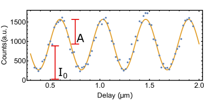
Figure S2: Sinusoidal envelope of the intensity on a single CCD pixel as a function of the piezo-controlled delay between the two arms of the interferometer.

The path length is scanned by sub-wavelength steps in order to extract the first order correlation function as:

$$|g^{(1)}(\mathbf{r},\mathbf{-r})|=VI_{\text{ideal}},$$ (S2)

where $I_{\text{ideal}}=\displaystyle(I_{1}+I_{2})(2\sqrt{I_{1}I_{2}})^{-1}$ takes into account small asymmetries between the two interferometer arms, with $I_{1}$ and $I_{2}$ the intensities in the two interferometer arms and $V$ is the visibility of the interference fringes obtained by fitting the data with:

$$I(x)=I_{0}+A\sin(\omega x+\phi_{0})$$ (S3)

where the visibility $V=\frac{A}{I_{0}}$ is shown in Fig. S2 and $\phi_{0}$ is the initial phase.

Coherence Length and Time

In order to evaluate the coherence length and time as a function of density, both spatial $g^{(1)}(x,-x,t=0)$ and temporal $g^{(1)}(t,t+\Delta t)$ are fitted with stretched exponentials as reported in Eq. (2) of the main text. It is therefore possible to define both in space and time the relaxation length (time) as:

$$\langle l\rangle=\int_{0}^{\infty}dxe^{-(x/l_{e})^{\beta}}=\frac{l_{e}}{\beta}\Gamma\left(\frac{1}{\beta}\right)$$ (S4)

with $l_{e}$ the renormalization factor scale of the x-axis and $\Gamma$ the gamma function, with x-axis both the spatial and temporal one. The resulting coherence length and time are reported in Fig. S3:

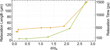
Figure S3: Coherence length (yellow) and time (green) for different densities extracted from the stretched exponential fitting.

Fitting Model and Residuals Analysis

The analysis of the fitting results allows to assess the applicability of the model used in the fitting procedure. In Fig. S4 we show the residuals of fitting the temporal first order correlation function $g^{(1)}(t,t+\Delta t)$ in the quasi-ordered regime (Red square in Fig. 3h of the main paper). We report different attempts to fit the data using an exponential (blue, row (a)), a Gaussian (yellow, row (b)), a stretched exponential (green, row (c)) and a power law (red, row (d)). The P-P (Probability Probability) plot is a standard tool to investigate the deviance of a data set from the normal distribution.

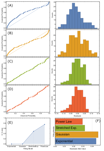
Figure S4: Fitting residuals analysis for the temporal algebraic regime (red square in Fig. 3h of the main text). Each color corresponds to a different model used to fit the temporal decay. Row a: P-P plot for the observed and expected Gaussian with minimum standard deviation of residuals distribution for the exponential model. Row b: Gaussian model. Row c: Stretched exponential model. Row d: Power law model. e: Kolmogorov-Smirnov value quantifying the normality of the residuals distribution for each model. f: Total Absolute Value of fitting residuals, normalised to the number of point used.

Indeed, fitting residuals with a normal distribution around the zero value represents a strong indication that the power-law model used to fit the data is the best one. The Kolmogorov-Smirnov test permits to quantitatively check the deviation from the normal distribution of a dataset. In order to assure that we have the minimum residual spreading, we used a normalised Gaussian distribution with $\sigma$ the minimum from the residuals distributions for each model fitting the experimental data. The value of this test, maximum for the power law model, combined with the fact (Fig. S4f) that the sum of the absolute values of the residuals is minimum for the power law model, confirms that the power law is the best fitting for the temporal decay of the correlation above BKT transition. In Fig. S5 we show the same analysis for the same regime (red square in Fig. 3g of the main paper but for the spatial decay of correlations. In this case the Gaussian fitting is not shown because the values of the residuals is too large.

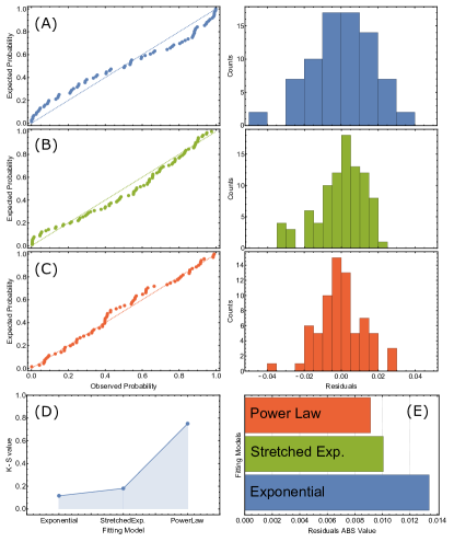
Figure S5: Fitting residuals analysis for the spatial algebraic regime (red square in Fig. 3g of the main text). Each color corresponds to a different model used to fit the spatial decay. Row a: P-P plot for the observed and expected Gaussian with minimum standard deviation of residuals distribution for the exponential model. Row b: Stretched exponential model. Row c: Ppower law model. d: Kolmogorov-Smirnov value quantifying the normality of the residuals distribution for each model. e: Total Absolute Value of fitting residuals, normalised to the number of point used.

Theoretical Description

In the classic equilibrium BKT scenario, for a system with linear dispersion in the ordered phase, we expect a slow algebraic decay (as eq. (1) of the main text) of the first order coherence with exactly the same power-law exponents in both space ($\alpha_{s}$) and time ($\alpha_{t}$) ^{2; 3}, given by $\alpha_{s,t}=k_{B}T/n_{s}$, where $T$ indicates temperature and $n_{s}$ the superfluid density. $\alpha_{s,t}$ have an upper bound of 1/4 ⁴ at which density/temperature vortices proliferate, causing an exponential decay of coherence, characteristic for the disordered phase. At the same time non-equilibrium dissipative driven systems, with diffusive spectrum in the ordered phase ^{2; 5}, have been shown to still exhibit an algebraic decay of coherence but with temporal correlations decaying two times slower then the spatial ones $\alpha_{t}=1/2\alpha_{s}$ ^{2; 3}. Moreover, values of $\alpha_{s}$ as large as four times the equilibrium upper bound, when approaching the BKT transition, were reported both experimentally ⁶ and from theoretical analysis ¹⁹, using beyond-mean-field truncated Wigner methods able to account for vortices, suggesting an “over-shaken” superfluid state ⁷. Finally, it has recently been suggested that the dissipation might in fact have an even more profound effect on the system with collective phase fluctuations destroying the algebraic order at long distances, leading to a stretched exponential decay of first order coherence characteristic of Kardar-Parisi-Zhang phase (KPZ)⁸. In that scenario the parameter $\beta$ of the stretched exponential (see Eqn. (2) of the main paper) are also different for space ($\beta\approx$ 0.78) and time ($\beta\approx$ 0.48). Even if later estimates of the KPZ length-scales appeared to be unrealistic, and the presence of free topological defects strongly hampers the possibility of the KPZ phase ⁹, the true nature of the 2D exciton-polariton phase transition and the resulting order is still at the center of an intense debate. Additionally, the type of the Renormalisation-Group (RG) analysis, which led to those conclusions ^{8; 9}, rely on the expansion in one over the mean-field density, and so are inadequate in describing the crossover region close to the phase transition. Thus, here, to specifically address the region close to the phase transition we restore to exact numerical solutions of the stochastic equations of motions, described in the next section.

Stochastic simulations

Our system consists of an ensemble of bosonic particles (the lower-polaritons) of mass $m$ and lifetime $2\kappa$, interacting via contact interactions $g$, and driven incoherently with pump of strength $\gamma$. The pumping saturation due to other processes is $\Gamma$. Using Keldysh field theory one can show that by including the classical fluctuations to all orders, but quantum fluctuations only to the second order (correct in the long-wavelength limit), and employing the MSR formalism, one can arrive at the stochastic equation for the field $\psi(\mathbf{r},t)$ (for review see ¹⁰). Alternative derivation, using the Focker-Plank equation for the Wigner function, aimed at numerical implementation on a finite spatial grid $dV$has been reviewed in ¹¹. The finite grid version reads

$$id\psi(\mathbf{r},t)=\biggl{[}-\frac{\nabla^{2}}{2m}+g|\psi(\mathbf{r},t)|_{-}^{2}+(\gamma-\kappa-\Gamma|\psi(\mathbf{r},t)|_{-}^{2})\biggr{]}\psi(\mathbf{r},t)dt+dW$$ (S5)

where $dW$ is the Wiener noise with correlations

$$\left\langle dW^{*}(\mathbf{r^{\prime}},t)dW(\mathbf{r},t)\right\rangle=\frac{\gamma+\kappa+\Gamma|\psi(\mathbf{r},t)|_{-}^{2}}{dV}\delta_{\mathbf{r},\mathbf{r^{\prime}}}dt,$$

where by $|\psi(\mathbf{r},t)|_{-}$ we abbreviated the following expression for the density $|\psi(\mathbf{r},t)|_{-}=|\psi(\mathbf{r},t)|-\frac{1}{dV}$, which comes from the Wigner function relating to the time symmetric and not time ordered operators. In Ref. ⁸ the Eqn. (S5) is solved approximately analytically using RG analysis by eliminating the amplitude fluctuations, and focusing solely on the non-topological phase-fluctuations. The procedure, however, relies on an expansion in one over the mean-field density, which together with approximating the amplitude fluctuations and discarding vortices, cannot capture the region close to the phase transition. Instead, here, we solve this equation exactly numerically on a finite grid. In addition, we have checked our results with a more general model of a saturable drive, applicable up to higher densities, in which $\gamma-\Gamma|\psi(\mathbf{r},t)|_{-}^{2}$ in Eqn. (S5) is replaced by $\frac{\gamma}{1+\frac{|\psi(\mathbf{r},t)|_{-}^{2}}{n_{s}}}$ with the noise strength proportional to $\frac{\gamma}{1+\frac{|\psi(\mathbf{r},t)|^{2}_{-}}{n_{s}}}+\kappa$. There is no appreciable difference between the results from the two models for our relatively low densities.

We evolve the dynamics of the stochastic equations (S5) with the XMDS2 software ¹² using a fixed-step (to ensure stochastic noise consistency) 4th order Runge-Kutta (RK) algorithm, which we have tested against fixed-step 9th order RK, and a semi-implicit fixed-step algorithm with 3 and 5 iterations. We choose the system parameters the same as in the experimental part: the mass of the microcavity lower polaritons is taken to be $m_{C}=3.8\times 10^{-5}m_{e}$, where $m_{e}$ is the electron mass, the polariton lifetime $2\kappa=101.3ps$, and the polariton-polariton interaction strength $g=0.004$ meV$\mu$m². The only parameter not possible to extract from the experiment is the saturation rate of the driving process (or in other words the three-body type losses in the system). We perform analysis for a range of $\Gamma$ (or $n_{s}$) values, and since the other parameters are fixed, we choose the value of $\Gamma$ ($n_{s}$)to reproduce the overall length scale of $g^{(1)}(x)$.

In our method, the stochastic averages over the configurations of different realisations of the fields provide the expectation value of the corresponding symmetrically ordered operators, and it is important to get the results to converge in the number of realisations. The first order spatial correlation function $g^{(1)}(x)$ is evaluated according to Eq. (S1), by averaging over 100 independent stochastic paths, and additionally over auxiliary position in space $r_{0}$, since in simulations our system is uniform. The temporal correlation function is evaluated from a single spatial point (to avoid picking up any spatial correlations) after the steady-state is reached, and averaged over 10000 stochastic paths. Since the Wigner average provides the expectation value of the corresponding symmetrically (and not time)-ordered operators, we need to subtract the expectation value of the commutator. For single time correlation functions, such as $g^{(1)}(x)$, the commutator is simply $\frac{1}{2dV}$. For two-time correlation functions, such as $g^{(1)}(t)$, strictly speaking the expectation value of the commutator is unknown. It is, however, changing from $\frac{1}{2dV}$ at $t=0$ to $0$ at $t\to\infty$. Using the two limiting values allows us to estimate the error, which we expect to be small given the densities considered. Indeed, for the densities used here the difference is practically indistinguishable.

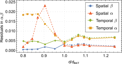
Figure S6: Residuals of the stretched exponential fit, $\beta$, for spatial (blue) and temporal (green) $g^{(1)}$, and the power-law fit, $\alpha$, for spatial (red) and temporal (orange) $g^{(1)}$ as a function of the polariton density normalised to the BKT threshold.

In order to test the robustness of our conclusions to the choice of the numerical parameters, we perform simulations on different spatial grids varying from 2 to $5\text{\,}\mathrm{\SIUnitSymbolMicro}\mathrm{m}$ in the grid spacing, and different system sizes from 256 to $1024\text{\,}\mathrm{\SIUnitSymbolMicro}\mathrm{m}$. Note, that to satisfy the condition necessary to derive the discrete version of equation (S5), $g/[(\kappa+\gamma)dV]\ll 1$, whilst maintaining a sufficient spatial resolution and, at the same time, a large enough momentum range, the window of available momentum grids is quite narrow. We find the main conclusions of our work (such as the crossover in $g^{(1)}(x)$ and $g^{(1)}(t)$ from exponential to power-law, spatial and temporal $\alpha$ being the same in the algebraic phase and smaller then 1/4, as well as the behaviour of vortices) independent on the choice of those parameters. Here, we present a case with $2\text{\,}\mathrm{\SIUnitSymbolMicro}\mathrm{m}$ grid spacing, and system size of $256\text{\,}\mathrm{\SIUnitSymbolMicro}\mathrm{m}$, which is sufficiently larger from experimental to avoid any boundary effects influencing the relevant region. Finally, in order to assess which functional form fits the numerical data best we perform residuals analysis similar to those applied to experimental data. The residuals for the data and fittings presented in the main text is shown in Fig S6.

References

References

- 1 H. E. Stanley, Scaling, universality, and renormalization: Three pillars of modern critical phenomena. Rev. Mod. Phys. 71, S358 (1999).
- 2 C. Castellano, S. Fortunato, V. Loreto, Statistical physics of social dynamics. Rev. Mod. Phys. 81, 591 (2009).
- 3 L. Onsager, Crystal statistics. I. A two-dimensional model with an order-disorder transition. Phys. Rev. 65, 117 (1944).
- 4 L. D. Landau, E. M. Lifshitz. Statistical Physics: Volume 5 (Course of Theoretical Physics) (Butterworth-Heinemann, 1980).
- 5 P. Hohenberg, B. Halperin, Theory of dynamic critical phenomena. Rev. Mod. Phys. 49, 435 (1977).
- 6 L. Pitaevskii, S. Stringari. Bose-Einstein Condensation and Superfluidity (Oxford University Press, 2016).
- 7 M. Kohl, T. Donner, S. Ritter, T. Bourdel, A. Ottl, F. Brennecke, T. Esslinger, Criticality and correlations in cold atomic gases. Advances in Solid State Physics 47, 79 (2008).
- 8 S. Braun, M. Friesdorf, M. Hodgman, S.S. Schreiber, P. Ronzheimer, A. Riera, M. Del Rey, I. Bloch, J. Eisert, U. Schneider, Emergence of coherence and the dynamics of quantum phase transitions. PNAS 112, 3641 (2015).
- 9 N. D. Mermin, H. Wagner, Absence of ferromagnetism or antiferromagnetism in one- or two-dimensional isotropic heisenberg models. Phys. Rev. Lett. 17, 1133 (1966).
- 10 P. Minnhagen, The two-dimensional coulomb gas, vortex unbinding, and superfluid-superconducting films. Rev. Mod. Phys. 59, 1001–1066 (1987).
- 11 J. Steinhauer, R. Ozeri, N. Katz, N. Davidson, Excitation spectrum of a bose-einstein condensate. Phys. Rev. Lett. 88, 120407 (2002).
- 12 D. R. Nelson, J. M. Kosterlitz, Universal jump in the superfluid density of two-dimensional superfluids. Phys. Rev. Lett. 39, 1201–1205 (1977).
- 13 M. H. Szymanska, J. Keeling, P. B. Littlewood, Nonequilibrium quantum condensation in an incoherently pumped dissipative system. Phys. Rev. Lett. 96, 230602 (2006).
- 14 M. H. Szymańska, J. Keeling, P. B. Littlewood, Mean-field theory and fluctuation spectrum of a pumped decaying bose-fermi system across the quantum condensation transition. Phys. Rev. B 75, 195331 (2007).
- 15 M. Richard, J. Kasprzak, R. Romestain, R. Andre, L. S. Dang, Spontaneous coherent phase transition of polaritons in CdTe microcavities. Phys. Rev. Lett. 94, 187401 (2005).
- 16 I. Carusotto, C. Ciuti, Quantum fluids of light. Rev. Mod. Phys. 85, 299 (2013).
- 17 E. Altman, L. M. Sieberer, L. Chen, S. Diehl, J. Toner, Two-dimensional superfluidity of exciton polaritons requires strong anisotropy. Phys. Rev. X 5, 011017 (2015).
- 18 G. Wachtel, L. Sieberer, S. Diehl, E. Altman, Electrodynamic duality and vortex unbinding in driven-dissipative condensates. arXiv:1604.01042v2 (2016).
- 19 G. Dagvadorj, J. M. Fellows, S. Matyjaskiewicz, F. M. Marchetti, I. Carusotto, M. H. Szymanska, Nonequilibrium phase transition in a two-dimensional driven open quantum system. Phys. Rev. X 5, 041028 (2015).
- 20 S. Utsunomiya, L. Tian, G. Roumpos, C. W. Lai, N. Kumada, T. Fujisawa, M. Kuwata-Gonokami, A. Loffler, S. Hofling, A. Forchel, Y. Yamamoto, Observation of Bogoliubov excitations in exciton-polariton condensates. Nature Phys. 4, 700 (2008).
- 21 V. Kohnle, Y. Léger, M. Wouters, M. Richard, M. T. Portella-Oberli, B. Deveaud-Plédran, From single particle to superfluid excitations in a dissipative polariton gas. Phys. Rev. Lett. 106, 255302 (2011).
- 22 V. Kohnle, Y. Léger, M. Wouters, M. Richard, M. T. Portella-Oberli, B. Deveaud, Four-wave mixing excitations in a dissipative polariton quantum fluid. Phys. Rev. B 86, 064508 (2012).
- 23 G. Roumpos, M. Lohse, W. H. Nitsche, J. Keeling, M. H. Szymanska, P. B. Littlewood, A. Löffler, S. Höfling, L. Worschech, A. Forchel, Y. Yamamoto, Power-law decay of the spatial correlation function in exciton-polariton condensates. Proceedings of the National Academy of Sciences 109, 6467–6472 (2012).
- 24 D. N. Krizhanovskii, D. Sanvitto, A. P. D. Love, M. S. Skolnick, D. M. Whittaker, J. S. Roberts, Dominant effect of polariton-polariton interactions on the coherence of the microcavity optical parametric oscillator. Phys. Rev. Lett. 97, 097402 (2006).
- 25 A. P. D. Love, D. N. Krizhanovskii, D. M. Whittaker, R. Bouchekioua, D. Sanvitto, S. A. Rizeiqi, R. Bradley, M. S. Skolnick, P. R. Eastham, R. Andre, L. S. Dang, Intrinsic decoherence mechanisms in the microcavity polariton condensate. Phys. Rev. Lett. 101, 067404 (2008).
- 26 S. Kim, B. Zhang, Z. Wang, J. Fischer, S. Brodbeck, M. Kamp, C. Schneider, S. Höfling, H. Deng, Coherent polariton laser. Phys. Rev. X 6, 011026 (2016).
- 27 S. Dihel, A. Micheli, A. Kantian, B. Kraus, H. Buchler, P. Zoller, Quantum states and phases in driven open quantum systems with cold atoms. Nat. Phys. 4, 878 (2008).
- 28 J. Keeling, M. H. Szymańska, P. B. Littlewood. Keldysh Green’s function approach to coherence in a non-equilibrium steady state: connecting Bose-Einstein condensation and lasing, 293–329 (Springer Berlin Heidelberg, Berlin, Heidelberg, 2010).
- 29 P. Kirton, J. Keeling, Nonequilibrium model of photon condensation. Phys. Rev. Lett. 111, 100404 (2013).
- 30 H. Deng, G. Weihs, D. Snoke, J. Bloch, Y. Yamamoto, Polariton lasing vs. photon lasing in a semiconductor microcavity. PNAS 100, 15318 (2003).
- 31 L. V. Butov, Solid-state physics: A polariton laser. Nature 447, 540–541 (2007).
- 32 J. Klaers, J. Schmitt, F. Vewinger, M. Weitz, Bose–einstein condensation of photons in an optical microcavity. Nature 468, 545 (2010).
- 33 Y. Sun, P. Wen, Y. Yoon, G. Liu, M. Steger, L. Pfeiffer, K. West, D. Snoke, K. Nelson, Bose-einstein condensation of long-lifetime polaritons in thermal equilibrium. arXiv:1601.02581 (2016).
- 34 A. Chiocchetta, I. Carusotto, Non-equilibrium quasi-condensates in reduced dimensions. EPL (Europhysics Letters) 102, 67007 (2013).
- 35 J. Keeling, L. Sieberer, E. Altman, L. Chen, S. Diehl, J. Toner, Superfluidity and phase correlations of driven dissipative condensates. arXiv preprint arXiv:1601.04495 (2016).
- 36 D. N. Krizhanovskii, K. G. Lagoudakis, M. Wouters, B. Pietka, R. A. Bradley, K. Guda, D. M. Whittaker, M. S. Skolnick, B. Deveaud-Pledran, M. Richard, R. Andre, L. S. Dang, Coexisting nonequilibrium condensates with long-range spatial coherence in semiconductor microcavities. Phys. Rev. B 80, 045317 (2009).
- 37 D. Sanvitto, D. N. Krizhanovskii, D. M. Whittaker, S. Ceccarelli, M. S. Skolnick, J. S. Roberts, Spatial structure and stability of the macroscopically occupied polariton state in the microcavity optical parametric oscillator. Phys. Rev. B 73, 241308(R) (2006).
- 38 H. Deng, G. S. Solomon, R. Hey, K. H. Ploog, Y. Yamamoto, Spatial coherence of a polariton condensate. Phys. Rev. Lett. 99, 126403 (2007).
- 39 W. H. Nitsche, N. Y. Kim, G. Roumpos, C. Schneider, M. Kamp, S. Höfling, A. Forchel, Y. Yamamoto, Algebraic order and the berezinskii-kosterlitz-thouless transition in an exciton-polariton gas. Phys. Rev. B 90, 205430 (2014).
- 40 Z. Hadzibabic, P. Kruger, M. Cheneau, B. Battelier, J. Dalibard, Berezinskii-kosterlitz-thouless crossover in a trapped atomic gas. Nature 441, 1118–1121 (2006).
- 41 L. V. Butov, A. V. Kavokin, The behaviour of exciton-polaritons. Nat Photon 6, 2–2 (2012).
- 42 B. Deveaud-Pledran, The behaviour of exciton-polaritons. Nat Photon 6, 205–205 (2012).
- 43 D. Ballarini, D. Caputo, C. Muñoz, M. De Giorgi, L. Dominici, M. Szymańska, W. K., L. Pfeiffer, G. G., F. Laussy, D. Sanvitto, Formation of a macroscopically extended polariton condensate without an exciton reservoir (2016). eprint 1609.05717.
- 44 R. Butté, G. Delalleau, A. I. Tartakovskii, M. S. Skolnick, V. N. Astratov, J. J. Baumberg, G. Malpuech, A. Di Carlo, A. V. Kavokin, J. S. Roberts, Transition from strong to weak coupling and the onset of lasing in semiconductor microcavities. Phys. Rev. B 65, 205310 (2002).
- 45 D. Bajoni, E. Semenova, A. Lemaitre, S. Bouchoule, E. Wertz, P. Senellart, J. Bloch, Polariton light-emitting diode in a gaas-based microcavity. Phys. Rev. B 77, 113303 (2008).
Acknowledgements
Funding from the POLAFLOW ERC Starting Grant is acknowledged. M. H. S. acknowledges support from EPSRC (Grants No. EP/I028900/2 and No. EP/K003623/2).

References

- Ballarini et al. 2016 D. Ballarini, D. Caputo, C. Muñoz, M. De Giorgi, L. Dominici, M. Szymańska, W. K., L. Pfeiffer, G. G., F. Laussy, et al. (2016), eprint 1609.05717.
- Szymanska et al. 2006 M. H. Szymanska, J. Keeling, and P. B. Littlewood, Phys. Rev. Lett. 96, 230602 (2006).
- Szymańska et al. 2007 M. H. Szymańska, J. Keeling, and P. B. Littlewood, Phys. Rev. B 75, 195331 (2007).
- Nelson and Kosterlitz 1977 D. R. Nelson and J. M. Kosterlitz, Phys. Rev. Lett. 39, 1201 (1977).
- Wouters and Carusotto 2007 M. Wouters and I. Carusotto, Phys. Rev. A 76, 043807 (2007).
- Roumpos et al. 2012 G. Roumpos, M. Lohse, W. H. Nitsche, J. Keeling, M. H. Szymanska, P. B. Littlewood, A. Löffler, S. Höfling, L. Worschech, A. Forchel, et al., Proceedings of the National Academy of Sciences 109, 6467 (2012).
- Dagvadorj et al. 2015 G. Dagvadorj, J. M. Fellows, S. Matyjaskiewicz, F. M. Marchetti, I. Carusotto, and M. H. Szymanska, Phys. Rev. X 5, 041028 (2015).
- Altman et al. 2015 E. Altman, L. M. Sieberer, L. Chen, S. Diehl, and J. Toner, Phys. Rev. X 5, 011017 (2015).
- Wachtel et al. 2016 G. Wachtel, L. Sieberer, S. Diehl, and E. Altman, arXiv:1604.01042v2 (2016).
- L. M. Sieberer 2015 S. D. L. M. Sieberer, M. Buchhold, arXiv:1512.00637 (2015).
- Carusotto and Ciuti 2013 I. Carusotto and C. Ciuti, Rev. Mod. Phys. (2013), eprint 1205.6500.
- Dennis et al. 2012 G. R. Dennis, J. J. Hope, and M. T. Johnsson, Comput. Phys. Commun. 184, 201 (2012), eprint 1204.4255.