Low-$\ell$ power suppression in punctuated inflation

Abstract

Motivated by Planck confirmation of an anomalously low value of the CMB temperature fluctuations up to multipole $\ell<40$, we in this paper try to explain such feature by investigating case of punctuated inflation scenario. This form of inflation potential is inspired by Minimal Super-symmetric Standard Model (MSSM) wherein suppression of curvature perturbation power at large scales is produced by introducing period of fast-roll phase of the inflation sandwiched between two stages of slow-roll phase.

We apply Markov Chain Monte Carlo analysis to determine posterior distribution and the best fit values of the model parameters using recent WMAP9 and Planck data. We show that WMAP9 and Planck results are consistent with each other and that with Planck data we obtain tighter constraints for punctuated inflation parameters. We find that punctuated inflation leads to better fit in CMB data compared to simple power law model. The improvement in the fit to the WMAP9 data is $\Delta\chi^{2}\sim 3.6$ and for Planck the improvement is $\Delta\chi^{2}\sim 5.4$. We find that $AIC$ does not discriminate between punctuated inflation and simple power law model for WMAP9 data. However, for Planck data we find that punctuated inflation is moderately preferred over a simple power law model.

1 Introduction

Anisotropy in the cosmic microwave background (CMB) is one of the most robust and informative tools in cosmology. Measurements of the CMB anisotropies by COBE, WMAP9 [1, 2] and Planck [3, 4] are in striking agreement with $\Lambda$CDM cosmology. These results are consistent with an adiabatic and nearly scale invariant spectrum of primordial perturbations, as predicted by the simple inflationary models [5, 6, 7]. The inflationary model(s) provide us potential solutions to most of the outstanding problems of standard Big Bang. They successfully explain the flatness problem, horizon problem and the monopole problem [5, 6, 8]. A key feature of these models is that during inflationary epoch, in the very early universe, primordial quantum fluctuations [9, 10, 11] of some scalar fields are produced which eventually transform into large scale structure of the universe under the gravitational instability paradigm. The observed statistical distribution of temperature fluctuations in the cosmic microwave background is believed to be sourced by these quantum fluctuations.

Although, power law (PL) model with almost scale-invariant, adiabatic and Gaussian primordial spectrum “$\mathcal{P}(k)$” ($k$ being the co-moving wavenumber) has emerged as the most successful model from the recent observations, there exist several anomalies in CMB data which could have far reaching consequences. Some of these anomalies are low CMB power at large angular scales [12, 13, 14, 15], departure from either Gaussianity or statistical isotropy [16, 17, 18, 19, 20, 21], lack of correlations on large scales [22, 23, 24], hemispheric asymmetry and the cold spot [25, 26, 27, 28, 29, 30], the so-called Axis of Evil [31, 32, 33] and oscillatory features in the primordial power spectrum [34, 35, 36, 37, 38, 39, 40, 41, 42]. Many inconsistencies in angular power spectrum have also been found between WMAP9 and Planck data [43, 44, 45]. Recently, Addison et al. [46] found internal inconsistencies between high ($\ell>1000$) and low ($\ell<1000$) multipoles in the Planck data. They suggest that tension in the Planck high $\ell$ spectrum is either due to an unlikely statistical fluctuation or unaccounted systematics in data. Similarly, Hazra & Shafieloo [47] found that Planck data is consistent with the concordance $\Lambda$CDM model only at 2-3$\sigma$ confidence level with an indication of lack of power at both high and low $\ell$’s with respect to concordance model. The study of these anomalies and their statistical significance is of utmost importance for cosmology as these results could test the $\Lambda$CDM model.

Lack of power at low CMB multipoles can be attributed to spatial curvature [48], non-trivial topology [49], violation of statistical anisotropies [16], hemispherical anisotropy and non-gaussianity [50, 51], bouncing inflation [52, 53], dark energy during the inflation [54], primordial micro black holes [55], loop quantum cosmology [56], string theory [57, 58, 59], non-attractor initial conditions [60] and so on. Besides, there exist many other classes of inflationary models which give rise to additional features in primordial power spectra compared to simple power law model. Exploring different inflationary models is still an interesting problem and could help us in explaining many anomalies. In our earlier work, we carried a detailed study of the inflationary models which could produce cut off in primordial power spectrum at low $k$ so as to reproduce necessary suppression in the CMB power spectrum up to multipoles $\ell\leq 40$ observed in the Planck data. We found marginal preference of the cut off parameters that describe the power suppression at low multipoles [15]. However, in all these models, we have to assume a specific pre-inflationary era (like kinetic or radiation dominated regime) and/or some special initial conditions to achieve a near scale invariant power spectrum along with a cut off at large scales (i.e low $k$). In this paper, we will consider punctuated inflationary scenario (PI model) which allows a brief period of fast roll sandwiched between two stages of slow roll inflation. Such scenario can be encountered in the Minimal Supersymmetric Standard Model (MSSM) wherein the inflationary potentials contain a point of inflection [61, 62, 63, 64, 65]. The break in the slow roll will induce power suppression followed by rise in the primordial power spectrum corresponding to the scales that leave the Hubble radius just before the transition to the fast roll [66, 67, 68]. The form of inflationary potential that we consider in this work has been previously investigated by Jain et al. [68, 69] using WMAP5 year data and this work can be regarded as a progression of their work. They showed that brief period of fast roll induces step like feature in the primordial spectrum corresponding to the Hubble scales leading to the suppression in the CMB power at low multipoles. Such scenario is advantageous in that we don’t have to consider any special pre-inflationary era or impose any special initial condition. Given the new Planck data and improved WMAP9 data, we aim to tighten the constraints on the parameter space with respect to previous work. Indeed, if the Planck and WMAP results are not consistent with each other then this would clearly imply the rejection of such model. Moreover, we also use Akaike information criterion ($AIC$) [70] to compare punctuated inflation model with PL model.

The plan of this paper is as follows: In section 2, we discuss punctuated inflationary model which can produce cut off primordial power spectrum at large scales. We then discuss CMB data set and methodology used in our analysis in section 3. In section 4, we give parameter estimates and explore Akaike information criterion for comparing punctuated inflationary model with power law model. Finally, we conclude our work in section 5. Throughout this work we will assume $\hbar=c=8\pi G=1$.

2 Punctuated inflation

The deviations from the scale invariance of the power spectrum can be produced by introducing two or more periods of fast roll phase. Such cases arise in double inflationary scenarios where one uses two scalar fields [71, 72, 73, 74]. Within single field inflationary scenarios, such departure from the slow roll phase are usually produced by introducing step or sudden change in slope of the inflationary field [75, 76, 77, 78]. However, there also exist many smooth and well behaved potentials that can incorporate fast roll phase [79, 66, 67]. The extent of deviations would depend on the nature and duration of the fast roll which are essentially controlled by the model parameters. The potential that we consider in this work to achieve a phase of fast roll is motivated by MSSM, an extension of the Standard Model (SM) which has many cosmological consequences [61, 62, 63, 64, 65]. In such scenarios, inflation carries the standard model (SM) charges and eventually decays into the SM baryons and the cold dark matter. We will consider following form of inflationary potential which has been earlier studied by Jain et al. [68, 69]

$$V(\phi)=\left(\frac{m^{2}}{2}\right)\,\phi^{2}-\left(\frac{\sqrt{2\,\lambda\,(n-1)}\,m}{n}\right)\,\phi^{n}+\left(\frac{\lambda}{4}\right)\,\phi^{2(n-1)},$$ (2.1)

where we consider the case $n=3$ and the coefficient of the $\phi^{n}$ term has been chosen in such a way that the potential has a point of inflection (point where both $V_{\phi}\equiv(dV/d\phi)$ and $V_{\phi\phi}\equiv(d^{2}V/d\phi^{2})$ vanish) at $\phi=\phi_{0}$ given by

$$\phi_{0}=\left(\frac{2\,m^{2}}{(n-1)\,\lambda}\right)^{\frac{1}{2\,(n-2)}}.$$ (2.2)

This form of the inflationary potential is shown in figure 1 using best fit parameters. It is important to note that in the usual Minimal Super-symmetric Standard Models, the point of inflection is located at the sub-Planckian values (i.e. $\phi_{0}<<1$). However, for our case the inflationary potential has an inflection at $\phi_{0}>>1$, if we have to induce a period of the fast roll followed by a second phase of slow roll. This is helpful in our case in the sense that the inflationary phase becomes independent of the initial value of the $\phi_{i}$ and $\dot{\phi}_{i}$ while in case of MSSM they have to be severely fine tuned; $\phi_{i}\sim\phi_{0}$ and $\dot{\phi}_{i}\sim 0$ [61]. It has been shown by Jain et al. [68] that if we start with any initial value $\phi_{i}>>\phi_{0}$ then the subsequent dynamics of the punctuated field approach the attractor and the attractor trajectory exhibit two regimes of slow roll inflation sandwiching a period of fast roll. It is worth mentioning that even though we consider the parameters of the inflationary potential that are different from the MSSM case, it may be possible to realize such scenarios beyond standard model (see [68] for more details).

It is often found that if we consider single field inflationary models along with the slow roll approximation then the amplitude of the scalar perturbations freezes after the modes leave the Hubble radius which can be expressed in terms of inflationary potential as follows [7, 80]

$${\cal P}_{S}(k)\simeq\left(\frac{1}{12\,\pi^{2}}\right)\,\left(\frac{V^{3}}{V_{\phi}^{2}}\right).$$ (2.3)

However, if we also consider an intermediate period of fast roll, it is found that the super-Hubble amplitude of the modes that exit the Hubble scale just before start of fast roll are enhanced compared to their value at Hubble exit. For modes that exit the Hubble scale during fast roll, the amplitudes are actually suppressed [66, 81, 67, 82, 14]. Further, the modes that leave well before and after fast roll remain unaffected.

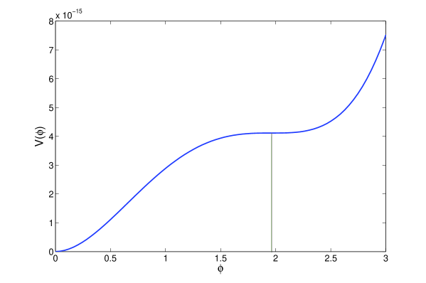
Figure 1: Form of the inflationary potential for parameters: $m=1.1323\times 10^{-7}$ and $\lambda=3.3299\times 10^{-15}$ (or $\phi_{0}=1.9622$). The vertical line represents the inflection point.

3 Solving primordial power spectrum

In this section, we will discuss equations of motion governing the evolution of scalar (curvature) perturbations and tensor perturbations. We use the formalism similar to Jain et al. [68], Aich et al. [38] and Hazra et al. [83] where they evolve the perturbations using the exact numerical approach using e-folds as the independent variable.

3.1 Background equations

The general action of scalar field in the curved space-time can be described by [84, 85]

$$S\,=-\,\int d^{4}\,x\,\sqrt{|g|}\,\left[\mathcal{L}_{g}+\mathcal{L}_{\phi}\,\right],$$ (3.1)

where

$$\mathcal{L}_{g}=\frac{1}{2}R,\quad\mathcal{L}_{\phi}=\frac{1}{2}g^{\mu\nu}\partial_{\mu}\phi\partial_{\nu}\phi-V(\phi),$$ (3.2)

are the Lagrangians for the gravitation and scalar fields respectively, $V(\phi)$ is the potential energy of the scalar field and $R$ is the curvature scalar. Variation of the action with respect to $\phi$ leads to the Klein-Gordon equation [85]

$$\frac{1}{\sqrt{|g|}}\partial_{\mu}\left[\sqrt{|g|}g^{\mu\nu}\partial_{\mu}\phi\right]+V_{\phi}=0.$$ (3.3)

For the spatially flat FRW metric where $g_{\mu\nu}=\textrm{diag}(1,-a^{2},-a^{2},-a^{2}$) and $\sqrt{|g|}=a^{3}$, $a$ being the scale factor, the above equation reduces to [8, 7]

$$\ddot{\phi}+3H\dot{\phi}-a^{-2}\nabla^{2}\phi+V_{\phi}=0,$$ (3.4)

where the overdots represent the differentiation with respect to cosmic time. The second term provides friction term for the scalar field which is proportional to the Hubble constant (expansion rate) $H=\dot{a}/a$ and third term is approximately equal to zero as the inflation would rapidly smooth out spatial variations in the universe. Similarly, variation of the action with respect to $g^{\mu\nu}$ gives us the Einstein tensor $G_{\mu\nu}$

$$G_{\mu\nu}=T_{\mu\nu},$$ (3.5)

where $T_{\mu\nu}$ is energy-momentum tensor of the scalar field given by,

$$T_{\mu\nu}=\partial_{\mu}\phi\partial_{\nu}\phi-g_{\mu\nu}\mathcal{L}_{\phi}.$$ (3.6)

For spatially flat FRW metric $T_{\mu\nu}$ reduces to [85]

$$T_{00}=\rho_{\phi}=\frac{1}{2}{\dot{\phi}}^{2}+V(\phi),\quad T_{ii}=p_{\phi}=\frac{1}{2}{\dot{\phi}}^{2}-V(\phi),$$ (3.7)

where $\rho_{\phi}$ and $p_{\phi}$ are the energy density and pressure density of the scalar field. The combination of $G_{00}$ and $G_{ii}$ provides a useful equation,

$$\dot{H}=\frac{1}{2}\dot{\phi}^{2},\quad 3H^{2}=\frac{1}{2}{\dot{\phi}}^{2}+V(\phi),$$ (3.8)

where the second equation is called the Friedmann equation. For inflation to happen, the scalar field is assumed to vary slowly with time (i.e $\dot{\phi}/2<<V$) which leads to the exponentially growing scale factor in the Friedmann equation. Slow-roll inflation is characterized by two parameters $\epsilon<<1$ and $\eta<<1$ which are defined as [6]

$$\epsilon=-\frac{\dot{H}}{H^{2}}=\frac{1}{2}\left(\frac{V_{\phi}}{V(\phi)}\right)^{2},\quad\eta=\epsilon+\delta=\left(\frac{V_{\phi\phi}}{V(\phi)}\right),$$ (3.9)

where $\delta=-\ddot{\phi}/H{\dot{\phi}}$.

3.2 Perturbation equations

In spatially flat Friedmann universe, the Fourier modes of the curvature perturbation $\mathcal{R}$ and the tensor perturbation $h$ are described by the following equations [80]

$$\mathcal{R}_{k}^{\prime\prime}+2\frac{z^{\prime}}{z}\mathcal{R}_{k}^{\prime}+k^{2}\mathcal{R}_{k}=0,\quad{h}_{k}^{\prime\prime}+2\frac{a^{\prime}}{a}{h}_{k}^{\prime}+k^{2}h_{k}=0,$$ (3.10)

where $z=a\dot{\phi}/H$ and the primes represent differentiation with respect to the conformal time. It is advantageous to consider the gauge invariant Mukhanov variables $u$ and $v$,

$$u=z\mathcal{R},\quad v=ah.$$ (3.11)

The Fourier components $u_{k}$ and $v_{k}$ obey the following equations of motion

$$u_{k}^{\prime\prime}+\left(k^{2}-\frac{z^{\prime\prime}}{z}\right)u_{k}=0,\quad v_{k}^{\prime\prime}+\left(k^{2}-\frac{a^{\prime\prime}}{a}\right)v_{k}=0,$$ (3.12)

We can then define the primordial power spectrum of curvature perturbations $\mathcal{P}_{s}(k)$ and tensor perturbations $\mathcal{P}_{t}(k)$ by the two-point correlation functions as [86]

$$<\mathcal{R}_{k_{1}}\mathcal{R}^{*}_{k_{2}}>=\frac{2\pi^{2}}{k^{3}}\mathcal{P}_{s}(k)\delta^{(3)}(k_{1}-k_{2}),\quad<{h}_{k_{1}}{h}^{*}_{k_{2}}>=\frac{2\pi^{2}}{k^{3}}\mathcal{P}_{t}(k)\delta^{(3)}(k_{1}-k_{2}).$$ (3.13)

Assuming Gaussianity and adiabaticity, $\mathcal{P}_{s}(k)$ and $\mathcal{P}_{t}(k)$ encode all the information for a complete statistical description of the fluctuations and are related to $u_{k}$ and $v_{k}$ via

$$\mathcal{P}_{s}(k)=\frac{k^{3}}{2\pi^{2}}\left|\frac{u_{k}}{z}\right|^{2},\quad\mathcal{P}_{t}(k)=2\frac{k^{3}}{2\pi^{2}}\left|\frac{v_{k}}{a}\right|^{2}.$$ (3.14)

Since, tensor-to-scalar ratio “$r$” remains smaller than $10^{-4}$ over whole cosmological scale for our model, therefore, we shall only consider scalar perturbation to minimize the computation time.

3.3 Initial conditions

In order to evaluate scalar power spectrum for different modes of $k$, we need to solve together background equation (equation 3.4) and perturbation equation (equation 3.10). Since both the equations are second order differential equations, we need 4 initial conditions - $\phi_{i}$, $\dot{\phi}_{i}$, $\mathcal{R}_{i}$ and $\mathcal{R^{\prime}}_{i}$. We assume $\phi_{i}$ to be equal to $12$ and $\dot{\phi}_{i}$ is evaluated using,

$$3H\dot{\phi}_{i}=-V(\phi_{i}).$$ (3.15)

The initial conditions for $\mathcal{R}_{i}$ and $\mathcal{R^{\prime}}_{i}$ can be obtained by imposing Bunch-Davies vacuum of de Sitter space when the perturbations are well inside the horizon,

$$\mathcal{R}_{i}=\frac{1}{\sqrt{2k}z_{i}}\exp(-ik\eta),$$ (3.16)

where conformal time $\eta$ is an irrelevant phase. In simple inflationary models, one usually imposes the initial conditions on the modes when $k/(aH)\approx 100$. Similarly, to compute the spectrum we need to integrate until the mode is far outside the horizon (i.e super-Hubble scales), typically, $k/aH\approx 10^{-5}$ [83, 68].

4 Methodology

4.1 CMB analysis

The initial power spectrum $\mathcal{P}(k)$ is related to the angular power spectrum $C_{\ell}$ through,

$$C_{\ell}^{{XX^{\prime}}}\propto\int{\rm d}{\rm ln}k\,\mathcal{P}(k)\,T_{\ell}^{X}(k)\,T_{\ell}^{X^{\prime}}(k),$$ (4.1)

where $T_{\ell}^{X}(k)$ is the transfer function with $X$ representing the CMB temperature or polarization. The measured angular power spectrum $C_{l}$ is a robust cosmological probe in constraining cosmological models, the position and amplitude of the peaks being very sensitive to important cosmological parameters.

We have used modified version of CAMB [87, 88] which is based on line of sight integration approach given in [89] to calculate the angular power spectra of the CMB anisotropies for different inflationary models discussed above. For exploring the likelihood function $\mathcal{L}(\mathbf{D}|\boldsymbol{\theta},\mathcal{M})$ (or the posterior distribution) of the parameters, we use Markov chain Monte Carlo (MCMC) methods. We have obtained the best fit values for the parameters using modified version of publicly available CosmoMC code [90] with a convergence diagnostics done through the Gelman and Rubins statistics. We have used PL model along with the PI derived scalar power spectrum for the cosmological estimates. We have conducted the analysis with two different data sets: WMAP9 and Planck. For WMAP9 data set, we have used full temperature and polarization 9 year data and likelihood code provided by the WMAP9 team. For Planck data set, we have used low $\ell$ TEB likelihood ($2\leq\ell\leq 29$) and high $\ell$ nuisance-marginalized Plik lite likelihood ($30\leq\ell\leq 2500$) to compute joint likelihood for TT, EE, BB, TE.

4.2 Model parameters and priors

The cosmological parameterization has been carried out by using the six basic parameters (baryon density ($\Omega_{b}h^{2}$), cold dark matter density ($\Omega_{c}h^{2}$), Thomson scattering optical depth due to re-ionization ($\tau$), angular size of horizon ($\theta$), scalar spectral index ($n_{s}$) and scalar amplitude ($\ln 10^{10}A_{s}$)) along with the three parameters which describe punctuated inflation ($\phi_{0}$, $\ln[10^{10}m^{2}]$) and scale factor of the universe at start of inflation ($a_{0}$). The remaining cosmological parameters are kept constant. We have fixed the sum of physical masses of standard neutrinos “$\nu"=0.06$ eV, effective number of neutrinos “Neff”$=3.046$, Helium mass fraction “YHe”$=0.24$ and the width of re-ionization $=0.5$. The results of the Bayesian parameter estimation may depend on the range of priors used. Table 1 shows the prior ranges of all parameters used in this work. Moreover, we have used flat prior distributions for all cosmological parameters.

Parameter Name	Symbol	Lower limit	Upper limit
Baryon density	$\Omega_{b}{h}^{2}$	0.005	0.1
Cold dark matter density	$\Omega_{c}{h}^{2}$	0.001	0.99
Angular size of acoustic horizon	$\theta$	0.5	10.0
Optical depth	$\tau$	0.01	0.8
Scalar spectral index	$n_{s}$	0.5	1.5
Scalar amplitude	$\ln[10^{10}A_{s}]$	2.7	4.0
Initial scale factor	$a_{0}$	0.0001	0.1
Inflection point	$\phi_{0}$	1.950	1.970
Inflationary mass	$\ln[10^{10}m^{2}]$	-12	-8

Table 1: Uniform prior used in parameter estimation.

		WMAP9			Planck
Model	Parameter	Best Fit	68% Limit	$\chi^{2}=-2\log{\mathcal{L}}$	Best Fit	68 % Limit	$\chi^{2}=-2\log{\mathcal{L}}$
PL	$\Omega_{b}{h}^{2}$	$0.0223$	$0.0223^{+0.0005}_{-0.0005}$	$7557.828$	$0.0211$	$0.0211^{+0.0001}_{-0.0001}$	$11629.944$
	$\Omega_{c}h^{2}$	$0.1141$	$0.1138^{+0.0046}_{-0.0044}$		$0.1239$	$0.1241^{+0.0015}_{-0.0015}$
	$\Omega_{\Lambda}$	$0.7110$	$0.7124^{+0.0288}_{-0.0234}$		$0.6521$	$0.6506^{+0.0107}_{-0.0105}$
	$\ln[10^{10}A_{s}]$	$3.0869$	$3.0878^{+0.0277}_{-0.0315}$		$3.0351$	$3.0421^{+0.0382}_{-0.0393}$
	$n_{s}$	$0.9670$	$0.9683^{+0.0126}_{-0.0127}$		$0.9483$	$0.9474^{+0.0046}_{-0.045}$
	$\tau$	$0.0861$	$0.0875^{+0.0127}_{-0.0147}$		$0.0500$	$0.0530^{+0.0193}_{-0.0196}$
	$100\theta$	$1.0393$	$1.0395^{+0.0057}_{-0.0073}$		$1.0400$	$1.0400^{+0.0003}_{-0.0003}$
	$z_{re}$	$10.551$	$10.617^{+1.112}_{-1.101}$		$7.5607$	$7.7661^{+2.3591}_{-1.936}$
	$H_{0}$	$68.898$	$69.158^{+5.517}_{-6.563}$		$64.738$	$64.662^{+0.673}_{-0.6609}$
PI	$\Omega_{b}{h}^{2}$	$0.0219$	$0.0220^{+0.0005}_{-0.0003}$	$7554.198$	$0.0211$	$0.0211^{+0.0001}_{-0.0001}$	$11624.540$
	$\Omega_{c}h^{2}$	$0.1172$	$0.1164^{+0.0041}_{-0.0045}$		$0.1247$	$0.1164^{+0.0016}_{-0.0016}$
	$\Omega_{\Lambda}$	$0.6914$	$0.6953^{+0.0273}_{-0.0218}$		$0.1040$	$0.6498^{+0.0109}_{-0.0110}$
	$\tau$	$0.0825$	$0.0826^{+0.0118}_{-0.0137}$		$0.6746$	$0.0571^{+0.0204}_{-0.0204}$
	$100\theta$	$1.0389$	$1.0387^{+0.0020}_{-0.0020}$		$1.0400$	$1.0400^{+0.0003}_{-0.0003}$
	$z_{re}$	$10.420$	$10.343^{+1.093}_{-1.083}$		$9.403$	$8.1973^{+2.4195}_{-1.9729}$
	$a_{0}$	$0.0097$	$0.0104^{+0.0041}_{-0.0066}$		$0.0070$	$0.0065^{+0.0020}_{-0.0019}$
	$\phi_{0}$	$1.9654$	$1.9661^{+0.0039}_{-0.0011}$		$1.9628$	$1.9630^{+0.0013}_{-0.0015}$
	$\ln[10^{10}m^{2}]$	$-9.8376$	$-10.137^{+0.626}_{-1.196}$		$-9.1350$	$-9.2039^{+0.3298}_{-0.4269}$
	$H_{0}$	$67.336$	$67.694^{+1.919}_{-1.738}$		$64.450$	$64.618^{+0.6591}_{-0.7400}$

Table 2: The best fit and mean values for power law (PL) model and Punctuated Inflation (PI) model obtained using WMAP9 year and Planck data sets.

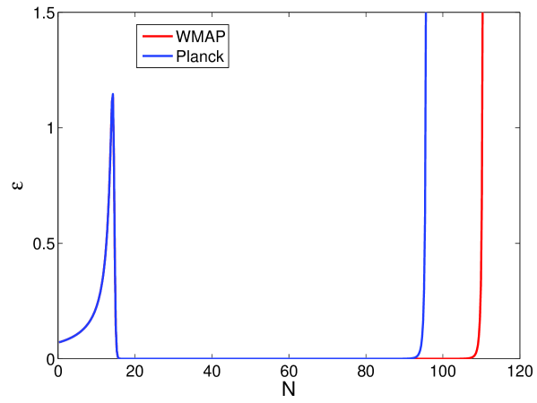
Figure 2: Evolution of the slow roll parameters $\epsilon$ as a function of e-folds $N$ in case of PI model for WMAP9 and Planck data. The slow roll approximation is violated (i.e $\epsilon>1$) for an e-fold around $N=13$ - $14$ e-folds. It can be seen that the evolution of $\epsilon$ is identical for WMAP9 and Planck data sets except at the late stage of inflation. Also note that here inflation ends at relatively large value of $N$ (i.e $N=112$ and $N=92$ for WMAP9 and Planck data sets respectively).

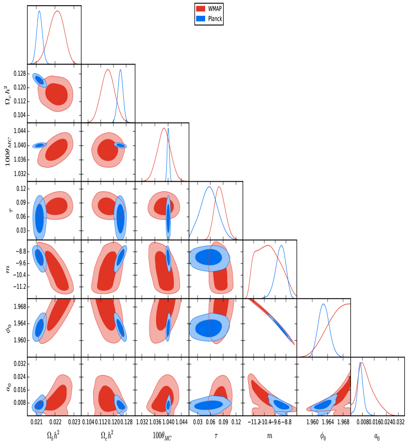
Figure 3: Two dimensional joint posterior probability distributions and one dimensional marginal posterior probability distribution for the parameters of the punctuated inflation along with other cosmological parameters.

5 Results and discussion

5.1 Best fit parameters and joint constraints

In table 2, we present the estimates of all the parameters in terms of the best fit values and their mean values with 1-$\sigma$ error bars for both PL model and PI model using WMAP9 and Planck data. Figure 2 shows the evolution of slow roll parameter $\epsilon$ as a function of e-folds $N$ for the best fit parameters of WMAP9 and Planck data set. As can be seen from figure 2, the slow roll approximation is violated for an e-fold around 13-14 e-folds. Figure 3 shows marginalized posterior distribution and two dimensional posterior distributions along with contours at 68% and 95% of the cosmological parameters for WMAP9 and Planck data set. Figure 4 shows best fit primordial spectra for PI model using WMAP9 and Planck data set. For comparison we have also plotted the best fit primordial power spectrum for the pure power law case. Figures 5 & 6 show the corresponding angular power spectra $C_{\ell}^{TT}$ for the best fit values of PI model parameters and other standard cosmological parameters.

From table 2, we see that PI model gives better fit to the data than the standard power law model at the cost of one extra parameter. For WMAP9 the improvement is $\Delta\chi^{2}\sim 3.6$ and for Planck data set the improvement in fit is $\Delta\chi^{2}\sim 5.4$. In the next section, we will discuss the significance of these fits using $AIC$. From figure 3, it is clear that we are able to obtain good bounds on all the parameters and that both WMAP9 and Planck data sets are consistent with each other. In fact, we were able to put tighter constraints on the parameters with the Planck data set. It follows from figure 4, that the main feature of the primordial power spectrum for PI model is the existence of sharp cut-off around $k\approx 4\times 10^{-4}$ followed by a bump around $k\approx 0.001$ and suppression around $k\approx 0.002$ in both WMAP9 and Planck cases. This corresponds to sharp cut-off in the $C_{\ell}^{TT}$ spectrum up to multipoles $\ell\leq 4$ followed by the bump ($5\leq\ell\leq 11$) and suppression ($12\leq\ell\leq 40$) as shown figure 5.

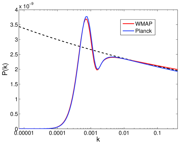
Figure 4: The best fit primordial spectra for PI model using WMAP9 (red line) and Planck (blue line) data sets. Note for both cases, we find sharp cut off around $k\approx 4\times 10^{-4}$ followed by a bump and suppression. At large $k$, PI primordial power spectrum matches with the standard power law model shown with the black dashed line.

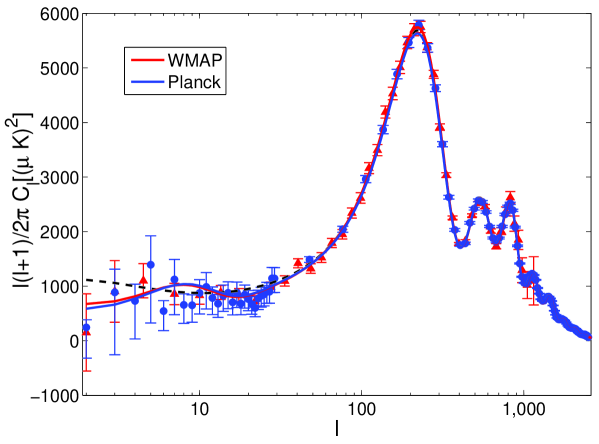
Figure 5: The best fit angular power spectra $C_{l}^{TT}$ for PI model using WMAP9 and Planck data sets. For comparison, we have also plotted $C_{l}^{TT}$ using power law model with black bashed line. The observed data points for WMAP9 and Planck data are also shown by red triangles and blue dots respectively.

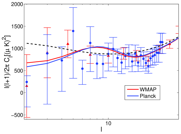
Figure 6: Same as in Fig. (5) at low-$\ell$. From this figure it is clear that the PI model induces power suppression up to a large values of $l\leq 40$ with a bump around $5\leq\ell\leq 11$ which results in the better improvement of fit in case of Planck data compared to WMAP9 data

.

5.2 Model comparison

To judge whether a model is preferred by data, we use Akaike information criterion ($AIC$) which incorporates trade-off between the goodness of fit and additional complexity of the model [70, 91, 92]:

$$AIC=-2\ln{\mathcal{L}_{max}}({\bf d}|{\bf\theta})+2N,$$ (5.1)

where $N$ is the number of free parameters and $\chi^{2}=-2\ln{\mathcal{L}_{max}}$, $\mathcal{L}_{max}$ being best fit likelihood value of the given model. In the above equation, first term represents the quality of the model fit and second term represent the model complexity. The $AIC$ is based on approximation to the Kullback-Leibler information entropy [93, 94]. The preferred model is the one which has a minimum value of $AIC$ and $\Delta AIC\equiv AIC_{i}-AIC_{min}$ represents preference of model $i$ over the best fit model (model with minimum value of $AIC$ i.e $AIC_{min}$). Models with $\Delta AIC\leq 2$ have substantial support, models with $4<\Delta AIC<7$ have considerably less support and those with $\Delta AIC>10$ have essentially no support compared to best fit model [95].

For Planck data set, we find $\Delta AIC=3.40$ which implies that PI model is moderately preferred compared to PL model despite having an additional parameter. However, for the WMAP9 only data set, we find that both models are equally favorable.

6 Conclusions

Although power law model has emerged as the most successful model consistent with recent observations, it could not explain certain anomalies. One of these anomalies is low CMB power at large angular scales in the CMB power spectrum. Different models have been used, having their own virtues and deficiencies, to account for this power loss. For example, in our previous work [15], we studied various inflationary models using different initial condition (like kinetic or radiation dominated era).

Motivated by the initial condition independence, in this work, we have used the punctuated inflationary model in which a brief period of fast roll is sandwiched between two stages of slow-roll inflation. Markov Chain Monte Carlo analysis has been performed to determine posterior distributions and the values of model parameters that provide best fit to WMAP9 and Planck data for CMB angular power spectrum. We found that PI model gives better fit to the data ($\Delta\chi^{2}\approx 3.6$ for WMAP9 and $\Delta\chi^{2}\approx 5.4$ for Planck) than the standard $\Lambda$CDM model with a featureless, primordial power spectrum at the cost of one extra parameter. Further, we used Akaki information criteria for model comparison which showed that for Planck data, PI model (having an additional parameter) is moderately preferred over PL model while as for WMAP9 data set only, both models are equally favorable.

There are models which superimpose oscillations on the power spectrum and which could produce $\Delta\chi^{2}\approx 10$ - $16$ [96, 97, 42]. However, in these cases the fitting is forced in the entire spectrum and the number of extra parameters involved are three or more. There also remains problem of over fitting data with such models. Similarly, many models have also been proposed with a step like feature in the inflationary potential [10, 75, 76] which are also found to better fit the data. Therefore, it is clear that significant improvement in both data and modeling is required to establish supremacy of one model over the other.

References

- [1] G. F. Smoot et al., Structure in the COBE differential microwave radiometer first-year maps, Astrophys. J. Lett. 396 (Sept., 1992) L1.
- [2] WMAP Collaboration, G. Hinshaw et al., Nine-Year Wilkinson Microwave Anisotropy Probe (WMAP) Observations: Cosmological Parameter Results, Astrophys. J. Lett. 208 (Oct., 2013) 19, [arXiv:1212.5226].
- [3] PLANCK Collaboration, P. A. R. Ade et al., Planck 2013 results. XVI. Cosmological parameters, Astronomy & Astrophysics 571 (Nov., 2014) A16, [arXiv:1303.5076].
- [4] PLANCK Collaboration, P. A. R. Ade et al., Planck 2015 results. XIII. Cosmological parameters, Astronomy & Astrophysics 594 (Sept., 2016) A13, [arXiv:1502.01589].
- [5] A. H. Guth, Inflationary universe: A possible solution to the horizon and flatness problems, Phys. Rev. D. 23 (Jan., 1981) 347.
- [6] A. R. Liddle, P. Parsons and J. D. Barrow, Formalizing the slow-roll approximation in inflation, Phys. Rev. D. 50 (Dec., 1994) 7222, [astro-ph/9408015].
- [7] A. R. Liddle and D. H. Lyth, Cosmological Inflation and Large-Scale Structure. Cambridge University Press, Apr., 2000.
- [8] A. R. Liddle and D. H. Lyth, The cold dark matter density perturbation, Phys. Rep. 231 (Aug., 1993) 1, [astro-ph/9303019].
- [9] S. W. Hawking, The development of irregularities in a single bubble inflationary universe, Physics Letters B 115 (Sept., 1982) 295.
- [10] A. A. Starobinsky, Dynamics of phase transition in the new inflationary universe scenario and generation of perturbations, Physics Letters B 117 (Nov., 1982) 175.
- [11] A. H. Guth and S.-Y. Pi, Fluctuations in the new inflationary universe, Physical Review Letters 49 (Oct., 1982) 1110.
- [12] J. R. Bond, A. H. Jaffe and L. Knox, Estimating the power spectrum of the cosmic microwave background, Phys. Rev. D. 57 (Feb., 1998) 2117, [astro-ph/9708203].
- [13] R. Sinha and T. Souradeep, Post-WMAP assessment of infrared cutoff in the primordial spectrum from inflation, Phys. Rev. D. 74 (Aug., 2006) 043518, [astro-ph/0511808].
- [14] M. Cicoli, S. Downes, B. Dutta, F. G. Pedro and A. Westphal, Just enough inflation: power spectrum modifications at large scales, JCAP 12 (Dec., 2014) 030, [arXiv:1407.1048].
- [15] A. Iqbal, J. Prasad, T. Souradeep and M. A. Malik, Joint Planck and WMAP Assessment of Low CMB Multipoles, JCAP 06 (June, 2015) 14, [arXiv:1501.02647].
- [16] A. Hajian and T. Souradeep, Measuring the Statistical Isotropy of the Cosmic Microwave Background Anisotropy, Astrophys. J. Lett. 597 (Nov., 2003) L5–L8, [astro-ph/0308001].
- [17] D. Seery and J. E. Lidsey, Non-Gaussianity from the inflationary trispectrum, JCAP 01 (Jan., 2007) 008, [astro-ph/0611034].
- [18] M. Aich and T. Souradeep, Statistical isotropy violation of the CMB brightness fluctuations, Phys. Rev. D. 81 (Apr., 2010) 083008, [arXiv:1001.1723].
- [19] PLANCK Collaboration, P. A. R. Ade et al., Planck 2013 results. XXIII. Isotropy and statistics of the CMB, Astronomy & Astrophysics 571 (Nov., 2014) A23, [arXiv:1303.5083].
- [20] P. K. Aluri, N. Pant, A. Rotti and T. Souradeep, Novel approach to reconstructing signals of isotropy violation from a masked CMB sky, Phys. Rev. D. 92 (Oct., 2015) 083015, [arXiv:1506.00550].
- [21] C. T. Byrnes and E. R. M. Tarrant, Scale-dependent non-Gaussianity and the CMB power asymmetry, JCAP 07 (July, 2015) 007, [arXiv:1502.07339].
- [22] C. J. Copi, D. Huterer, D. J. Schwarz and G. D. Starkman, Uncorrelated universe: Statistical anisotropy and the vanishing angular correlation function in WMAP years 1 3, Phys. Rev. D. 75 (Jan., 2007) 023507, [astro-ph/0605135].
- [23] C. J. Copi, D. Huterer, D. J. Schwarz and G. D. Starkman, Large-angle cosmic microwave background suppression and polarization predictions, Mon. Not. R. Astron. Soc. 434 (Oct., 2013) 3590, [arXiv:1303.4786].
- [24] A. Gruppuso, Two-point correlation function of Wilkinson Microwave Anisotropy Probe 9-yr data, Mon. Not. R. Astron. Soc. 437 (Jan., 2014) 2076, [arXiv:1310.2822].
- [25] H. K. Eriksen, F. K. Hansen, A. J. Banday, K. M. Gorski and P. B. Lilje, Asymmetries in the Cosmic Microwave Background Anisotropy Field, Astrophys. J. 605 (Apr., 2004) 14, [astro-ph/0307507].
- [26] F. K. Hansen, A. J. Banday and K. M. Górski, Testing the cosmological principle of isotropy: local power-spectrum estimates of the WMAP data, Mon. Not. R. Astron. Soc. 354 (Nov., 2004) 641, [astro-ph/0404206].
- [27] J. A. R. Cembranos, A. de la Cruz-Dombriz, A. Dobado and A. L. Maroto, Is the CMB cold spot a gate to extra dimensions?, JCAP 10 (Oct., 2008) 039, [arXiv:0803.0694].
- [28] Y. Akrami, Y. Fantaye, A. Shafieloo, H. K. Eriksen, F. K. Hansen, A. J. Banday and K. M. Górski, Power Asymmetry in WMAP and Planck Temperature Sky Maps as Measured by a Local Variance Estimator, Astrophys. J. Lett. 784 (Apr., 2014) L42, [arXiv:1402.0870].
- [29] H. Assadullahi, H. Firouzjahi, M. H. Namjoo and D. Wands, CMB hemispherical asymmetry from non-linear isocurvature perturbations, JCAP 04 (Apr., 2015) 017, [arXiv:1410.8036].
- [30] PLANCK Collaboration, P. A. R. Ade et al., Planck 2015 results. XVI. Isotropy and statistics of the CMB, Astronomy & Astrophysics 594 (Aug., 2016) A16, [arXiv:1506.07135].
- [31] K. Land and J. Magueijo, Examination of Evidence for a Preferred Axis in the Cosmic Radiation Anisotropy, Phys. Rev. Lett. 95 (Aug., 2005) 071301, [astro-ph/0502237].
- [32] M. Frommert and T. A. Enßlin, The axis of evil - a polarization perspective, Mon. Not. R. Astron. Soc. 403 (Apr., 2010) 1739, [arXiv:0908.0453].
- [33] A. Rassat, J.-L. Starck, P. Paykari, F. Sureau and J. Bobin, Planck CMB anomalies: astrophysical and cosmological secondary effects and the curse of masking, JCAP 08 (Aug., 2014) 006, [arXiv:1405.1844].
- [34] C. Pahud, M. Kamionkowski and A. R. Liddle, Oscillations in the inflaton potential?, Phys. Rev. D. 79 (Apr., 2009) 083503, [arXiv:0807.0322].
- [35] R. Flauger, L. McAllister, E. Pajer, A. Westphal and G. Xu, Oscillations in the CMB from axion monodromy inflation, JCAP 06 (July, 2010) 009, [arXiv:0907.2916].
- [36] T. Kobayashi and F. Takahashi, Running spectral index from inflation with modulations, JCAP 01 (Jan., 2011) 026, [arXiv:1011.3988].
- [37] P. Adshead, C. Dvorkin, W. Hu and E. A. Lim, Non-Gaussianity from step features in the inflationary potential, Phys. Rev. D. 85 (Jan., 2012) 023531, [arXiv:1110.3050].
- [38] M. Aich, D. K. Hazra, L. Sriramkumar and T. Souradeep, Oscillations in the inflaton potential: Complete numerical treatment and comparison with the recent and forthcoming CMB datasets, Phys. Rev. D. 87 (Apr., 2010) 083526, [arXiv:1106.2798].
- [39] H. V. Peiris, R. Easther and R. Flauger, Constraining monodromy inflation, JCAP 09 (Sept., 2013) 018, [arXiv:1303.2616].
- [40] M. Benetti, Updating constraints on inflationary features in the primordial power spectrum with the Planck data, Phys. Rev. D. 88 (Oct., 2013) 087302, [arXiv:1308.6406].
- [41] PLANCK Collaboration, P. A. R. Ade and et al., Planck 2013 results. XXII. Constraints on inflation, Astronomy & Astrophysics 571 (Nov., 2014) A22, [arXiv:1303.5082].
- [42] PLANCK Collaboration, P. A. R. Ade et al., Planck 2015 results. XX. Constraints on inflation, Astronomy & Astrophysics 594 (Sept., 2016) A20, [arXiv:1502.02114].
- [43] D. K. Hazra and A. Shafieloo, Test of consistency between Planck and WMAP, Phys. Rev. D. 89 (Jan., 2014) 043004, [arXiv:1308.2911].
- [44] D. Larson, J. L. Weiland, G. Hinshaw and C. L. Bennett, Comparing Planck and WMAP: Maps, Spectra, and Parameters, Astrophys. J. 801 (Mar., 2015) 9, [arXiv:1409.7718].
- [45] A. Shafieloo, Crossing statistic: reconstructing the expansion history of the universe, JCAP 08 (Aug., 2012) 002, [arXiv:1204.1109].
- [46] G. E. Addison, Y. Huang, D. J. Watts, C. L. Bennett, M. Halpern, G. Hinshaw and J. L. Weiland, Quantifying discordance in the 2015 Planck CMB spectrum, Astrophys. J. 818 (Feb., 2016) 132, [arXiv:1511.00055].
- [47] D. K. Hazra and A. Shafieloo, Confronting the concordance model of cosmology with Planck data, JCAP 1 (Jan., 2014) 43, [arXiv:1401.0595].
- [48] G. Efstathiou, Is the low cosmic microwave background quadrupole a signature of spatial curvature?, Mon. Not. R. Astron. Soc. 343 (Aug., 2003) L95–L98, [astro-ph/0303127].
- [49] J.-P. Luminet, J. R. Weeks, A. Riazuelo, R. Lehoucq and J.-P. Uzan, Dodecahedral space topology as an explanation for weak wide-angle temperature correlations in the cosmic microwave background, Nature. 425 (Oct., 2003) 593–595, [astro-ph/0310253].
- [50] J. McDonald, Hemispherical power asymmetry from a space-dependent component of the adiabatic power spectrum, Phys. Rev. D. 89 (June, 2014) 127303, [arXiv:1403.2076].
- [51] J. McDonald, Negative running of the spectral index, hemispherical asymmetry and the consistency of Planck with large r, JCAP 11 (Nov., 2014) 012, [arXiv:1403.6650].
- [52] Y.-S. Piao, B. Feng and X. Zhang, Suppressing the CMB quadrupole with a bounce from the contracting phase to inflation, Phys. Rev. D. 69 (May, 2004) 103520, [hep-th/0310206].
- [53] Z.-G. Liu, Z.-K. Guo and Y.-S. Piao, Obtaining the CMB anomalies with a bounce from the contracting phase to inflation, Phys. Rev. D. 88 (Oct., 2013) 063539, [arXiv:1304.6527].
- [54] C. Gordon and W. Hu, Low CMB quadrupole from dark energy isocurvature perturbations, Phys. Rev. D. 70 (Oct., 2004) 083003, [astro-ph/0406496].
- [55] F. Scardigli, C. Gruber and P. Chen, Black hole remnants in the early universe, Phys. Rev. D. 83 (Mar., 2011) 063507, [arXiv:1009.0882].
- [56] A. Barrau, T. Cailleteau, J. Grain and J. Mielczarek, Observational issues in loop quantum cosmology, Classical and Quantum Gravity 31 (Mar., 2014) 053001, [arXiv:1309.6896].
- [57] E. Dudas, N. Kitazawa, S. P. Patil and A. Sagnotti, CMB imprints of a pre-inflationary climbing phase, JCAP 5 (May, 2012) 012, [arXiv:1202.6630].
- [58] N. Kitazawa and A. Sagnotti, A string-inspired model for the low- CMB, Mod. Phys. Lett. 30 (July, 2015) 1550137, [arXiv:1503.04483].
- [59] Y.-F. Cai, E. G. M. Ferreira, B. Hu and J. Quintin, Searching for features of a string-inspired inflationary model with cosmological observations, Phys. Rev. D. 92 (Dec., 2015) 121303, [arXiv:1507.05619].
- [60] Y.-F. Cai, J.-O. Gong, D.-G. Wang and Z. Wang, Features from the non-attractor beginning of inflation, JCAP 10 (Oct., 2016) 017, [arXiv:1607.07872].
- [61] R. Allahverdi, K. Enqvist, J. Garcia-Bellido and A. Mazumdar, Gauge-invariant inflaton in the minimal supersymmetric standard model, Phys. Rev. Lett. 97 (Nov., 2006) 191304, [hep-ph/0605035].
- [62] R. Allahverdi, K. Enqvist, J. Garcia-Bellido, A. Jokinen and A. Mazumdar, MSSM flat direction inflation: slow roll, stability, fine-tuning and reheating, JCAP 06 (June, 2007) 019, [hep-ph/0610134].
- [63] J. C. Bueno Sanchez, K. Dimopoulos and L. D. H., A-term inflation and the minimal supersymmetric standard model, JCAP 01 (Jan., 2007) 015, [hep-ph/0608299].
- [64] R. Allahverdi, S. Downes and B. Dutta, Constructing Flat Inflationary Potentials in Supersymmetry, Phys. Rev. D. 84 (Nov., 2011) 101301, [arXiv:1106.5004].
- [65] S. Choudhury, A. Mazumdar and S. Pal, Low & high scale MSSM inflation, gravitational waves and constraints from Planck, JCAP 07 (July, 2013) 041, [arXiv:1305.6398].
- [66] S. M. Leach, M. Sasaki, D. Wands and A. R. Liddle, Enhancement of superhorizon scale inflationary curvature perturbations, Phys. Rev. D. 64 (July, 2001) 023512, [astro-ph/0101406].
- [67] R. K. Jain, P. Chingangbam and L. Sriramkumar, On the evolution of tachyonic perturbations at super-Hubble scales, JCAP 10 (Oct., 2007) 003, [astro-ph/0703762].
- [68] R. K. Jain, P. Chingangbam, J.-O. Gong, L. Sriramkumar and T. Souradeep, Punctuated inflation and the low CMB multipoles, JCAP 1 (Jan., 2009) 009, [arXiv:0809.3915].
- [69] R. K. Jain, P. Chingangbam, L. Sriramkumar and T. Souradeep, Tensor-to-scalar ratio in punctuated inflation, Phys. Rev. D. 82 (July, 2010) 023509, [arXiv:0904.2518].
- [70] H. Akaike, A new look at the statistical model identification, Automatic Control, IEEE Transactions on 19 (Dec., 1974) 716.
- [71] D. Polarski and A. A. Starobinsky, Structure of primordial gravitational waves spectrum in a double inflationary model, Phy. Lett. B 356 (Feb., 1995) 196, [astro-ph/9505125].
- [72] J. A. Adams, G. G. Ross and S. Sarkar, Multiple inflation, Nucl. Phys. B 503 (Feb., 1997) 405, [hep-ph/9704286].
- [73] S. Tsujikawa, D. Parkinson and B. A. Bassett, Correlation-consistency cartography of the double-inflation landscape, Phys. Rev. D. 67 (Apr., 2003) 083516, [astro-ph/0210322].
- [74] S. Schettler and J. Schaffner-Bielich, Model with two periods of inflation, Phys. Rev. D. 93 (Jan., 2016) 025001, [arXiv:1510.00557].
- [75] J. Adams, B. Cresswell and R. Easther, Inflationary perturbations from a potential with a step, Phys. Rev. D. 64 (Dec., 2001) 123514, [astro-ph/0102236].
- [76] J.-O. Gong, Breaking scale invariance from a singular inflaton potentia, JCAP 07 (July, 2005) 015, [astro-ph/0504383].
- [77] J. Martin, L. Sriramkumar and D. K. Hazra, Sharp inflaton potentials and bi-spectra: effects of smoothening the discontinuity, JCAP 09 (Sept., 2014) 039, [arXiv:1404.6093].
- [78] Y.-F. Cai, F. Chen, E. G. M. Ferreira and J. Quintin, New model of axion monodromy inflation and its cosmological implications, JCAP 06 (June, 2016) 027, [arXiv:1412.4298].
- [79] H. M. Hodges, G. R. Blumenthal, L. A. Kofman and J. R. Primack, Nonstandard primordial fluctuations from a polynomial inflation potential, Nucl. Phys. B 335 (Apr., 1990) 197.
- [80] V. F. Mukhanov, H. A. Feldman and R. H. Brandenberger, Theory of cosmological perturbations, Phys. Rep. 215 (June, 1992) 203.
- [81] R. Saito, J. Yokoyama and R. Nagata, Single-field inflation, anomalous enhancement of superhorizon fluctuations and non-Gaussianity in primordial black hole formation, JCAP 06 (June, 2008) 024, [arXiv:0804.3470].
- [82] J. L. Cook and L. M. Krauss, Large slow roll parameters in single field inflation, JCAP 03 (Mar., 2016) 028, [arXiv:1508.03647].
- [83] D. K. Hazra, L. Sriramkumar and J. Martin, BINGO: A code for the efficient computation of the scalar bi-spectrum, JCAP 05 (May, 2013) 026, [arXiv:1201.0926].
- [84] S. Weinberg, Gravitation and Cosmology: Principles and Applications of the General Theory of Relativity. WILEY, July, 1972.
- [85] T. Padmanabhan, Gravitation: Foundations and Frontiers. Cambridge University Press, Jan., 2010.
- [86] R. Durrer, The Cosmic Microwave Background. Cambridge University Press, Cambridge, UK, Aug., 1998.
- [87] A. Lewis, A. Challinor and A. Lasenby, Efficient Computation of Cosmic Microwave Background Anisotropies in Closed Friedmann-Robertson-Walker Models, Astrophys. J. 538 (Aug., 2000) 473, [astro-ph/9911177].
- [88] A. Lewis and A. Challinor, Evolution of cosmological dark matter perturbations, Phys. Rev. D. 66 (July, 2002) 023531, [astro-ph/0203507].
- [89] U. Seljak and M. Zaldarriaga, A Line-of-Sight Integration Approach to Cosmic Microwave Background Anisotropies, Astrophys. J. 469 (Oct., 1996) 437, [astro-ph/9603033].
- [90] A. Lewis and S. Bridle, Cosmological parameters from CMB and other data: A Monte Carlo approach, Phys. Rev. D. 66 (Nov., 2002) 103511, [astro-ph/0205436].
- [91] A. R. Liddle, How many cosmological parameters?, Mon. Not. R. Astron. Soc. 351 (July, 2004) L49, [astro-ph/0401198].
- [92] C. R. Contaldi, M. Peloso, L. Kofman and A. Linde, Suppressing the lower multipoles in the CMB anisotropies, JCAP 7 (July, 2003) 002, [astro-ph/0303636].
- [93] D. R. Anderson and K. Burnham, Model selection and multimodel inference. Springer-Verlag, 2002.
- [94] G. Goswami and J. Prasad, Maximum entropy deconvolution of primordial power spectrum, Phys. Rev. D. 88 (July, 2013) 023522, [arXiv:1303.4747].
- [95] P. B. Kenneth and R. A. David, Model Selection and Multimodel Inference: A Practical Information-Theoretic Approach. Springer Science and Business Media, 2002.
- [96] P. D. Meerburg, D. N. Spergel and B. D. Wandelt, Searching for oscillations in the primordial power spectrum. II. Constraints from the Planck data, Phys. Rev. D. 89 (Mar., 2014) 063537, [arXiv:1308.3705].
- [97] P. D. Meerburg, D. N. Spergel and B. D. Wandelt, Searching for oscillations in the primordial power spectrum. I. Perturbative approach, Phys. Rev. D. 89 (Mar., 2014) 063536, [arXiv:1308.3704].