Analytic solution for Gauged Dirac-Weyl equation in $(2+1)$-dimensions

Abstract

A gauged Dirac-Weyl equation in (2+1)-dimension is considered. This equation has the particularity to describe the states of a graphene Dirac matter. In particular we are interested in matter interacting with a Chern-Simons gauge fields. We show that exact self-dual solutions are admitted. These solutions are the same as those supported by nonrelativistic matter interacting with a Chern-Simons gauge field.

PACS numbers: 11.10.Kk, 11.15.Yc, 81.05.ue

1 Introduction

The two dimensional matter field interacting with gauge fields whose dynamics is governed by a Chern-Simons term support soliton solutions[1, 18, 3, 4, 5, 6, 7]. These models have the particularity to became auto-dual when the self-interactions are suitably chosen [8, 9, 10, 11]. When this occur the model presents particular mathematical and physics properties, such as the supersymmetric extension of the model [12], and the reduction of the motion equation to first order derivative equation [13]. The Chern-Simons gauge field inherits its dynamics from the matter fields to which it is coupled, so it may be either relativistic [8] or non-relativistic [10, 11]. In addition the soliton solutions are of topological and non-topological nature [14].
In the present Letter, we investigate Dirac-Weyl massless fermions under perpendicular magnetic field whose dynamics is dictated by a Chern-Simons gauge field. In particular we show that this gauge theory admit soliton solutions which are analytic and coincide with the self-dual solutions supported by Schrödinger-Chern-Simons model [10, 11] defined by the Lagrangian density

$$\mathcal{L}=\frac{\kappa}{2}\epsilon^{\mu\nu\rho}A_{\mu}\partial_{\nu}A_{\rho}+i\psi^{*}D_{0}\psi-\frac{1}{2m}|D_{i}\psi|^{2}+\frac{g}{2}|\psi|^{4}$$ (1)

where, the first term is a Chern-Simons gauge field dynamics, which are coupled to nonrelativistic bosonic matter, represented by the complex scalr field $\psi$.

2 The soliton solution

Let us start by considering a $(2+1)$-dimensional Dirac-Weyl-Chern-Simons model coupled to two-component spinors

$$\Psi=(\psi_{a},\psi_{b})^{T}$$ (2)

where $\psi_{a}$ and $\psi_{b}$ represent the envelope functions associated with the probability amplitudes. In addition, T denotes the transpose of the column vector. Then the action is governed by

$$S=\int d^{3}x\Big{(}\frac{\kappa}{2}\epsilon^{\mu\nu\rho}A_{\mu}\partial_{\nu}A_{\rho}+\Psi^{\dagger}\sigma^{0}D_{0}\Psi-\Psi^{\dagger}\sigma^{i}D_{i}\Psi\Big{)}$$ (3)

Here, the covariant derivative is defined as $D_{0}=-i\partial_{0}-eA_{0}$, $D_{i}=-i\partial_{i}+eA_{i}$ $(i=1,2)$, the metric tensor is $g^{\mu\nu}=(-1,1,1)$ and $\epsilon^{\mu\nu\lambda}$ is the totally antisymmetric tensor such that $\epsilon^{012}=1$. Also, $\sigma^{\mu}$ $(\mu=0,1,2)$ are 2$\times$2 Pauli matrices, i.e.

$$\sigma^{0}=\left(\begin{array}[]{cc}1&0\\ 0&1\end{array}\right)\,,\;\;\;\;\;\ \sigma^{1}=\left(\begin{array}[]{cc}0&1\\ 1&0\end{array}\right)\,,\;\;\;\;\;\ \sigma^{2}=\left(\begin{array}[]{cc}0&-i\\ i&0\end{array}\right)$$ (10)

The Chern-Simons term of the action (3) may be developed integrating by parts,

$$S_{cs}=\frac{\kappa}{2}\int d^{3}x\Big{(}\epsilon^{\mu\nu\rho}A_{\mu}\partial_{\nu}A_{\rho}\Big{)}=\kappa\int d^{2}x\Big{(}A_{0}F_{12}+A_{2}\partial_{0}A_{1}\Big{)}$$ (11)

On the plane the curl of a vector is a scalar, so that the magnetic field is $F_{12}=\partial_{1}A_{2}-\partial_{2}A_{1}$. We may also develop the Dirac-Weyl term,

$$S_{dw} = \int d^{3}x\Big{(}\Psi^{\dagger}\sigma^{0}D_{0}\Psi-\Psi^{\dagger}\sigma^{i}D_{i}\Psi\Big{)}$$ (12)

$$= \int d^{3}x\Big{(}-i\psi_{a}^{\dagger}\partial_{0}\psi_{a}-eA_{0}\psi_{a}^{\dagger}\psi_{a}-i\psi_{b}^{\dagger}\partial_{0}\psi_{b}-eA_{0}\psi_{b}^{\dagger}\psi_{b}-[-i\psi_{a}^{\dagger}\partial_{1}\psi_{b}-\psi_{a}^{\dagger}\partial_{2}\psi_{b}$$

$$+eA_{1}\psi_{a}^{\dagger}\psi_{b}-ieA_{2}\psi_{a}^{\dagger}\psi_{b}-i\psi_{b}^{\dagger}\partial_{1}\psi_{a}+\psi_{b}^{\dagger}\partial_{2}\psi_{a}+eA_{1}\psi_{b}^{\dagger}\psi_{a}+ieA_{2}\psi_{b}^{\dagger}\psi_{a}]\Big{)}$$

Then, the corresponding field equations for the action (3) are

$$- i\partial_{0}\psi_{a}-eA_{0}\psi_{a}-[-i\partial_{1}\psi_{b}-\partial_{2}\psi_{b}+eA_{1}\psi_{b}-ieA_{2}\psi_{b}]$$ (13)

$$= D_{0}\psi_{a}-[D_{1}\psi_{b}-iD_{2}\psi_{b}]=0$$

$$- i\partial_{0}\psi_{b}-eA_{0}\psi_{b}-[-i\partial_{1}\psi_{a}+\partial_{2}\psi_{a}+eA_{1}\psi_{a}-ieA_{2}\psi_{a}]$$ (14)

$$= D_{0}\psi_{b}-[D_{1}\psi_{a}+iD_{2}\psi_{a}]=0$$

$$\kappa F_{12}-e[\psi^{\dagger}_{a}\psi_{a}+\psi^{\dagger}_{b}\psi_{b}]=0$$ (15)

$$\kappa(-\partial_{0}A_{2}+\partial_{2}A_{0})-e[\psi^{\dagger}_{a}\psi_{b}+\psi^{\dagger}_{b}\psi_{a}]=0$$ (16)

$$\kappa(\partial_{0}A_{1}-\partial_{1}A_{0})-e[-i\psi^{\dagger}_{a}\psi_{b}+i\psi^{\dagger}_{b}\psi_{a}]=0$$ (17)

The equations (13) and (14) may be expressed in a compact form as

$$\sigma^{0}D_{0}\Psi-\sigma^{i}D_{i}\Psi=0$$ (18)

which is the massless Dirac-Weyl equation in (2+1)-dimensions. This equation is gauge invariant since a gauge transformation of the potentials,

$$A_{i}\rightarrow A_{i}-\frac{1}{e}\partial_{i}\omega\,,\;\;\;\;\;\ A_{0}\rightarrow A_{0}+\frac{1}{e}\partial_{0}\omega$$ (19)

accompanied by a transformation of the spinor

$$\Psi\rightarrow e^{i\omega}\Psi$$ (20)

leaves the equation (18) unchanged.
The gauge field satisfied its dynamical equations, which are dictated by the formulas (15), (16) and (17). These are the Chern-Simons field equations coupled to matter field by $j^{0}=e[\psi^{\dagger}_{a}\psi_{a}+\psi^{\dagger}_{b}\psi_{b}]$ and $j^{i}=e\psi^{\dagger}\sigma^{i}\psi$, which are the conserved currents associated to gauge symmetry (20). So that,

$$\partial_{\mu}j^{\mu}=\partial_{0}j^{0}+\partial_{i}j^{i}=0$$ (21)

In particular, the field equations (15), (16) and (17) may be reduced to a single equation

$$\frac{\kappa}{2}\epsilon^{\nu\alpha\beta}F_{\alpha\beta}=j^{\nu}$$ (22)

Thus, the equation (15) is the time component of this equation

$$\kappa F_{12}=j^{0}$$ (23)

Then, integrating over the entire plane, we obtain the important consequence that any field configuration with charge $Q=\int d^{2}xj^{0}$ also carries magnetic flux $\Phi=\int Bd^{2}x$ [15, 16, 17]:

$$\Phi=\frac{1}{\kappa}Q$$ (24)

In addition, the equations (16) and (17) are the spatial components of (22),

$$j^{i}=\epsilon^{ij}\kappa E_{j}$$ (25)

In this note we will show that the system (3) admit a static soliton solution carrying magnetic flux and electric charge. In order to show this we consider the stationary points of the action which for the static field configuration reads

$$S=\int d^{2}x\Big{(}\kappa A_{0}F_{12}-eA_{0}(\psi_{a}^{\dagger}\psi_{a}+\psi_{b}^{\dagger}\psi_{b})-[-i\psi_{a}^{\dagger}\partial_{1}\psi_{b}-\psi_{a}^{\dagger}\partial_{2}\psi_{b}+eA_{1}\psi_{a}^{\dagger}\psi_{b}$$

$$-ieA_{2}\psi_{a}^{\dagger}\psi_{b}-i\psi_{b}^{\dagger}\partial_{1}\psi_{a}+\psi_{b}^{\dagger}\partial_{2}\psi_{a}+eA_{1}\psi_{b}^{\dagger}\psi_{a}+ieA_{2}\psi_{b}^{\dagger}\psi_{a}]\Big{)}$$ (26)

In view of Gauss law constraint (23), the action may be rewritten as

$$S=-\int d^{2}x\Big{(}-i\psi_{a}^{\dagger}\partial_{1}\psi_{b}-\psi_{a}^{\dagger}\partial_{2}\psi_{b}+eA_{1}\psi_{a}^{\dagger}\psi_{b}-ieA_{2}\psi_{a}^{\dagger}\psi_{b}$$

$$-i\psi_{b}^{\dagger}\partial_{1}\psi_{a}+\psi_{b}^{\dagger}\partial_{2}\psi_{a}+eA_{1}\psi_{b}^{\dagger}\psi_{a}+ieA_{2}\psi_{b}^{\dagger}\psi_{a}\Big{)}$$

$$=-\int d^{2}x\Big{(}\psi_{a}^{\dagger}[D_{1}\psi_{b}-iD_{2}\psi_{b}]+\psi_{b}^{\dagger}[D_{1}\psi_{a}+iD_{2}\psi_{a}]\Big{)}$$ (27)

To proceed, we can use the static version of equations (13) and (14), i.e.,

$$\psi_{a}=\frac{-1}{eA_{0}}[D_{1}\psi_{b}-iD_{2}\psi_{b}]$$ (28)

$$\psi_{b}=\frac{-1}{eA_{0}}[D_{1}\psi_{a}+iD_{2}\psi_{a}]$$ (29)

So, the equation (27) reads

$$S = \int d^{2}x\frac{1}{eA_{0}}\Big{(}[D_{1}\psi_{b}-iD_{2}\psi_{b}]^{\dagger}[D_{1}\psi_{b}-iD_{2}\psi_{b}]+[D_{1}\psi_{a}+iD_{2}\psi_{a}]^{\dagger}[D_{1}\psi_{a}+iD_{2}\psi_{a}]\Big{)}$$ (30)

$$= \int d^{2}x\frac{1}{eA_{0}}\Big{(}|D_{1}\psi_{b}-iD_{2}\psi_{b}|^{2}+|D_{1}\psi_{a}+iD_{2}\psi_{a}|^{2}\Big{)}$$

Since, $A_{0}$ is a Lagrange multiplier, which does not play any role in the search of static solution, we can choose, without loss of generality, $A_{0}>0$. Thus, the action (30) is non-negative and bounded below by zero. This lower bound is saturated by solutions to the first-order self-duality equations

$$(D_{1}-iD_{2})\psi_{b}=0$$

$$(D_{1}+iD_{2})\psi_{a}=0$$ (31)

Together with the Gauss law (23) these two equations compose the set of the field equations whose solutions minimize the static action (26). In particular, an interesting situation emerge when one of the spinor component is set to zero. In that case, the set of equations reduces to the self-duality equations of the Schrödinger-Chern-Simons model present in Ref.[10, 11],

$$(D_{1}+iD_{2})\psi_{a}=0$$

$$\kappa F_{12}=e\psi^{\dagger}_{a}\psi_{a}$$ (32)

with $\psi_{b}=0$ or

$$(D_{1}-iD_{2})\psi_{b}=0$$

$$\kappa F_{12}=e\psi^{\dagger}_{b}\psi_{b}$$ (33)

with $\psi_{a}=0$. Both, (32) and (33) may be solved analytically. We can take the set (32). To solve these equations is usual to decompose the scalar field $\psi_{a}$ into its phase and magnitude:

$$\psi_{a}=\rho^{\frac{1}{2}}e^{i\alpha}$$ (34)

where, $\rho=\psi^{\dagger}_{a}\psi_{a}$. Then, multiplying the first of the self-duality equations (32) by $i\psi^{\dagger}_{a}$ and its complex conjugate by $-i\psi_{a}$ we arrive to

$$i\psi^{\dagger}_{a}(D_{1}+iD_{2})\psi_{a}-i\psi_{a}[(D_{1}+iD_{2})\psi_{a}]^{\dagger}=2ieA_{2}|\psi_{a}|^{2}-2|\psi_{a}|^{2}i\partial_{2}\alpha+i\partial_{1}|\psi_{a}|^{2}=0$$ (35)

$$i\psi^{\dagger}_{a}(D_{1}+iD_{2})\psi_{a}+i\psi_{a}[(D_{1}+iD_{2})\psi_{a}]^{\dagger}=2ieA_{1}|\psi_{a}|^{2}-2|\psi_{a}|^{2}i\partial_{1}\alpha-i\partial_{2}|\psi_{a}|^{2}=0$$ (36)

This, determines the gauge field

$$A_{i}=\frac{1}{2e\rho}\Big{(}\epsilon^{ij}\partial_{j}(\log\rho)-2\partial_{i}\alpha\Big{)}$$ (37)

everywhere away from the zeros of the scalar field. Thus, using (37) the second self-duality equation of (32) reduces to a nonlinear elliptic equation for the scalar field density $\rho$,

$$\nabla^{2}\log\rho=-\frac{2e^{2}}{\kappa}\rho$$ (38)

We can proceed in similar way and take the set (33). Then, we arrive to

$$\nabla^{2}\log\rho=\frac{2e^{2}}{\kappa}\rho$$ (39)

These are elliptic equations, known as the Liouville equations and are exactly solvable,

$$\rho=\frac{\kappa}{e^{2}}\nabla^{2}\log\Big{(}1+|f|^{2}\Big{)}$$ (40)

where $f=f(z)$ is a holomorphic function of $z=x_{1}+ix_{2}$. General radially symmetric solutions may be obtained by taking $f(z)=\Big{(}\frac{z_{0}}{z}\Big{)}^{N}$. Then, we have

$$\rho=\frac{4\kappa N^{2}}{e^{2}r_{0}^{2}}\frac{\Big{(}\frac{r}{r_{0}}\Big{)}^{2(N-1)}}{\Big{(}1+(\frac{r}{r_{0}})^{2N}\Big{)}^{2}}$$ (41)

This vanish as $r\to\infty$ and is nonsingular at the origin for $|N|\geq 0$ but for $|N|>0$, the vector potential behaves as $A_{i}(r)\sim-\partial_{i}\alpha-2(N-1)\epsilon_{ij}\frac{x^{j}}{r^{2}}$, which indicates that it has a singular contribution at $r=0$. The singularity may be avoided if we choose the phase of $\phi$ to be $\alpha=\theta(N-1)$. Then, the self-dual $\phi$ field is (see figure 1)

$$\phi=\frac{\sqrt{\kappa}2N}{er_{0}}\Big{(}\frac{(\frac{r}{r_{0}})^{N-1}}{1+(\frac{r}{r_{0}})^{2N}}\Big{)}e^{-i(N-1)\theta}$$ (42)

Requiring that $\phi$ be single-valued we find that $N$ must be an integer, and for $\rho$ to decay at infinity we require that $N$ be positive.
To conclude it is interesting to comment that the solution (42) is the same as the soliton solution discussed in Ref.[10, 11]. In fact, as we mentioned, the self-duality equations (32) and (33) coincide with the self-duality equations of the Schrödinger-Chern-Simons model present in Ref.[10, 11]. The reason for this lies in the fact that the static Hamiltonian associated to the model (1) is

$$H=\int\,\,d^{2}x \Big{(}\frac{1}{2m}|D_{i}\psi|^{2}-\frac{g}{2}|\psi|^{4}\Big{)}$$ (43)

The static solutions, which are the stationary points of the Hamiltonian, may be found in view of the Chern-Simons Gauss law $B=\frac{e}{\kappa}\rho$ and the identity

$$|D_{i}\psi|^{2}=|(D_{1}\pm iD_{2})\psi|^{2}\mp eB|\psi|^{2}\pm m\epsilon^{ij}\partial_{i}J_{j}$$ (44)

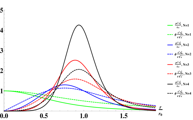
Figure 1: Scalar field density $\rho$ and self-dual field $\phi$ as a function of $r/r_{0}$ for different values of $N$ and $\theta=0$.

Then, (43) reads as

$$H=\int\,\,d^{2}x \Big{(}\frac{1}{2m}|(D_{1}\pm iD_{2})\psi|^{2}\pm\frac{\epsilon^{ij}}{2}\partial_{i}J_{j}+[-\frac{g}{2}\mp\frac{e^{2}}{2m\kappa}]|\psi|^{4}\Big{)}$$ (45)

Here, the second term in (45) is a surface term. To see this, we can apply the Stokes’ theorem, then we have,

$$\int\,\,d^{2}x\epsilon^{ij}\partial_{i}J_{j}=\oint_{|x|=\infty}\,\,J_{j}dx^{j}$$ (46)

where, $J_{j}=-\frac{i}{2m}\Big{(}\phi^{*}D_{j}\phi-(D_{j}\phi)^{*}\phi\Big{)}$. The requirement that the energy be finite states that the covariant derivative must vanish asymptotically. This fixes the behavior of the field at infinity. In the case of a nontopological theory such as the Jackiw-Pi model [10, 11], this implies the following boundary condition,

$$\lim_{r\to\infty}\phi(x)=0$$ (47)

whereas the gauge field, at infinity, is a pure gauge. Hence, $J_{j}\to 0$ as $x\to\infty$. Thus, with the self-dual coupling

$$g=\mp\frac{e^{2}}{m\kappa}$$ (48)

and sufficiently well behaved fields so that the integral over all space of $\epsilon^{ij}\partial_{i}J_{j}$ vanishes, the energy becomes

$$E=\int\,\,d^{2}x \frac{1}{2m}|(D_{1}\pm iD_{2})\psi|^{2}$$ (49)

If we compare this expression with (30) we note that they are very similar. So, the fields that minimize the energy (49) are the same as minimize (30) and therefore obey the equations (32) and (33). Thus, the identity (44) plays and important role in order to connect the Dirac model with a non-relativistic model.
In summary, we show that the Dirac-Weyl field interacting with gauge fields governed by Chern-Simons dynamics, support analytic static self-dual solutions. The solutions that we found are the same as the solution supported by nonrelativistic matter interacting with a Chern-Simons gauge fields. In addition, it well know [18]-[26] that in the low energy electronic excitations of graphene, an expansion around any of the two fermi points gives an effective Hamiltonian linear in momentum which reduces to the massless Dirac equation in two dimensions derived from the Hamiltonian,

$$H=\upsilon_{F}\int d^{2}x\Big{(}\Psi^{\dagger}\sigma^{i}\partial_{i}\Psi\Big{)}$$ (50)

where $\upsilon_{F}=8\times 10^{5}m/sec$ is the Fermi velocity. This Hamiltonian is associated to a static field configuration and therefore it can be derived from a more general Hamiltonian for time dependent fields

$$H=\upsilon_{F}\int d^{3}x\Big{(}-\Psi^{\dagger}\sigma^{0}D_{0}\Psi+\Psi^{\dagger}\sigma^{i}D_{i}\Psi\Big{)}$$ (51)

which is the Hamiltonian for the description of a graphene layer in presence of electric and magnetic fields (see for instance [27, 28, 29, 30, 31, 32, 33, 34]).
On the other hand, Chern-Simons term becomes important in the description of fractional quantum Hall effect (FQHE) in graphene [35, 36, 37, 39, 40, 41, 42, 43]. A way to understand the nature of these states is provided by the composite Fermion(CF) theory [44] in which the state of the system is described in terms of CF quasiparticles which correspond to electrons bound to an even number (2k) of vortices of flux quantum $\Phi_{0}=\frac{hc}{e}$. Such a flux attachment can also be understood by carrying out Chern-Simon (CS) transformation on the electron field operators, which leads to the introduction of a topological CS vector potential a resulting in a CS magnetic field, which is proportional to the electron density $j^{0}=e[\psi^{\dagger}_{a}\psi_{a}+\psi^{\dagger}_{b}\psi_{b}]$ [45, 46]. In other words, the dynamics of the magnetic field is dictated by the Chern-Simons Gauss law (23). Thus, the Chern-Simons term is important because allows us to introduce a general flux tied to the electrons, and then it has its own dynamics. In particular, many works have been done in the study of graphene Dirac electrons interacting with an external magnetic field [47]-[56]. In general numerical computation is required and some simple cases for an electron in the presence magnetic field are solve analytically [54, 56]. In this direction, we think that our result may be important because constitutes an exact solution for the description of graphene Dirac electrons in a magnetic field with its own gauge dynamics dictated by a Chern-Simons term.

Acknowledgements

This paper was partially supported by grants of CONICET (Argentina National Research Council) and Universidad Nacional del Sur (UNS)and by ANPCyT through PICT 1770, and PIP-CONICET Nos. 114-200901-00272 and 114-200901-00068 research grants, as well as by SGCyT-UNS., A. J., J. S. A. and L. S. are members of CONICET.