Statistical Learning Theory Approach for Data Classification with $\ell$-diversity

Abstract

Corporations are retaining ever-larger corpuses of personal data; the frequency or breaches and corresponding privacy impact have been rising accordingly. One way to mitigate this risk is through use of anonymized data, limiting the exposure of individual data to only where it is absolutely needed. This would seem particularly appropriate for data mining, where the goal is generalizable knowledge rather than data on specific individuals. In practice, corporate data miners often insist on original data, for fear that they might ”miss something” with anonymized or differentially private approaches. This paper provides a theoretical justification for the use of anonymized data. Specifically, we show that a support vector classifier trained on anatomized data satisfying $\ell$-diversity should be expected to do as well as on the original data. Anatomy preserves all data values, but introduces uncertainty in the mapping between identifying and sensitive values, thus satisfying $\ell$-diversity. The theoretical effectiveness of the proposed approach is validated using several publicly available datasets, showing that we outperform the state of the art for support vector classification using training data protected by $k$-anonymity, and are comparable to learning on the original data.

1 Introduction

Many privacy definitions have been proposed based on generalizing/suppressing data ($\ell$-diversity[23], $k$-anonymity [27, 28], $t$-closeness [19], $\delta$-presence [25], ($\alpha$,$k$)-anonymity [32]). Other alternatives include value swapping [24], distortion [2], randomization [12], and noise addition (e.g., differential privacy [11]). Generalization consists of replacing identifying attribute values with a less specific version [28]. Suppression can be viewed as the ultimate generalization, replacing the identifying value with an “any” value [28]. Generalization has the advantage of preserving truth, but a less specific truth that reduces utility of the published data.

Xiao and Tao proposed anatomization as a method to enforce $\ell$-diversity while preserving specific data values [33]. Anatomization splits instances across two tables, one containing identifying information and the other containing private information. The more general approach of fragmentation [7] divides a given dataset’s attributes into two sets of attributes (2 partitions) such that an encryption mechanism avoids associations between two different small partitions. Vimercati et al. extend fragmentation to multiple partitions [9], and Tamas et al. propose an extension that deals with multiple sensitive attributes [13]. The main advantage of anatomization/fragmentation is that it preserves the original values of data; the uncertainty is only in the mapping between individuals and sensitive values.

We show that this additional information has real value. First, we demonstrate that in theory, learning from anatomized data can be as good as learning from the raw data. We then demonstrate empirically that learning from anatomized data beats learning from generalization-based anonymization.

This paper looks at linear support vector (SVC) and support vector machine (SVM) classifiers. This focus was chosen because these classifiers have a wide range of successful applications, and also have some solid theoretical basis their generalization properties. We propose a simple heuristic to preprocess the anatomized data such that SVC and SVM generalize well with sufficiently large training data.

There is concern that anatomization is vulnerable to several attacks [18, 14, 21]. While this can be an issue, any method that provides meaningful utility fails to provide perfect privacy against a sufficiently strong adversary [20, 11]. Introducing uncertainty into the anonymization process reduces the risk of many attacks, e.g., minimality [31, 8]. Our theoretical analysis holds for any assignment of items to anatomy groups, including a random assignment, which provides a high degree of robustness against minimality and correlation-based attacks. While this does not eliminate privacy risk, if the alternative is to use the original data, we show that anatomy provides comparable utility while reducing the privacy risk. This paper has the following key contributions:

1. We define a classification task on anatomized data without violating the random worlds assumption. A violating classification task would be the prediction of sensitive attribute, a task that was found to be #P-complete by Kifer [18].

2. We propose a heuristic algorithm to train SVC and SVM when the test data is neither anonymized nor anatomized. Inan et al. already gives a practical applications of such a learning scenario [15].

3. We study the effect of our heuristic algorithm on the generalization error. To our best knowledge, this is the first paper in the privacy community that does such analysis for $\ell$-diversity

4. In empirical analysis, our algorithm will be compared with SVM and SVC that are trained on either unprotected data or generalized data (under $k$-anonymity [15]). The analysis will be justified with the statistical learning theory [29, 5]

We next summarize related work and define the problem statement. We then give necessary definitions and notations. Section 4 proposes the heuristic algorithm and gives theoretical analysis. Empirical analysis is presented in section 5. Section 6 summarizes the work and gives future directions.

2 Related Work and Problem Statement

There have been studies of linear classification for anonymized data. Agrawal et al. proposed an iterative distribution reconstruction algorithm for distorted training data from which a C4.5 decision tree classifier was trained [1]. Iyengar suggested using a classification metric so as to find the optimum generalization. Then, a C4.5 decision tree classifier was trained from the optimally generalized training data [16]. Dowd et al. studied C4.5 decision tree learning from training data perturbed by random substitutions. A matrix based distribution reconstruction algorithm was applied on the perturbed training data from which an accurate C4.5 decision tree classifier was learned [10]. Inan et al. proposed support vector machine classifiers using anonymized training data that satisfy $k$-anonymity. Taylor approximation was used to estimate the linear and RBF kernel computation from generalized data[15]. Rubinstein et al. studies the kernels of support vector machine in the differential privacy and show the trade-off between privacy level and the data utility. They analyze finite and infinite dimensional kernels in function of the approximation error under differential privacy [26]. Lin at al. studies training support vector classification for outsourced data. Random transformation is applied on the training set so that the cloud server computes the accurate model without knowing what the actual values are [22]. Jain et al. studies the support vector machine kernels in the differential privacy setting. They propose differentially private mechanisms to train support vector machines for interactive, semi-interactive and non-interactive learning scenarios, providing theoretical analysis of the proposed approaches [17].

None of the earlier work has provided a linear classifier directly applicable to anatomized training data. Such a classifier requires specific theoretical and experimental analysis, because anatomized training data provides additional detail that has the potential to improve learning; but also additional uncertainty that must be dealt with. Furthermore, most of the previous work didn’t justify theoretically why the proposed heuristics let classifiers generalize well. Therefore, this paper studies the following problem: Define a heuristic to train SVCs and SVMs on anatomized data without violating $\ell$-diversity while using the sensitive information, with a theoretical guarantee of good generalization under reasonable assumptions.

3 Definitions and Notations

The first four definitions restate standard definitions of unprotected data and attribute types.

Definition 1

A dataset ${D}$ is called a person specific dataset for population ${P}$ if each instance ${X_{\_}i\in D}$ belongs to a unique individual ${p\in P}$.

The person specific dataset will be called the original training data in this paper. Next, we will give the first type of attributes.

Definition 2

A set of attributes are called direct identifying attributes if they let an adversary associate an instance $X_{\_}i\in D$ to a unique individual $p\in P$ without any background knowledge.

Definition 3

A set of attributes are called quasi-identifying attributes if there is background knowledge available to the adversary that associates the quasi-identifying attributes with a unique individual $p\in P$.

We include both direct and quasi-identifying attributes under the name identifying attribute. First name, last name and social security number (SSN) are common examples of direct identifying attributes. Some common examples of quasi-identifying attributes are age, postal code, and occupation. Next, we will give the second type of attribute.

Definition 4

An attribute of instance $X_{\_}i\in D$ is called a sensitive attribute if we should protect against adversaries correctly inferring the value for an individual.

Patient disease and individual income are common examples of sensitive attributes. Unique individuals $p\in P$ typically don’t want these sensitive information to be revealed to individuals without a direct need to know that information. Provided an instance $X_{\_}i\in D$, the class label is denoted by $X_{\_}i.C$. We don’t consider the case where $C$ is sensitive, as this would make the purpose of classification to violate privacy. $C$ is neither sensitive nor identifying in this paper, although our analysis holds for $C$ being an identifying attribute.

Given the former definitions, we will next define the anonymized training data following the definition of $k$-anonymity [28].

Definition 5

A training dataset $D$ that satisfies the following conditions is said to be anonymized training data $D_{\_}k$ [28]:

1. The training data $D_{\_}k$ does not contain any unique identifying attributes.

2. Every instance $X_{\_}i\in D_{\_}k$ is indistinguishable from at least $(k-1)$ other instances in $D_{\_}k$ with respect to its quasi-identifying attributes.

Anatomy satisfies a slightly weaker definition; the indistinguishability applies only to sensitive data. This will be captured in Definitions 8-15.

In this paper, we assume that the anonymized training data $D_{\_}k$ is created according to a generalization based data publishing method. We next define the comparison classifiers.

Definition 6

A linear support vector classifier (SVC) that is trained on the anonymized training data $D_{\_}k$ is called the anonymized SVC. Similarly, a support vector machine (SVM) that is trained on the anonymized training data $D_{\_}k$ is called the anonymized SVM.

Definition 7

A linear support vector classifier (SVC) that is trained on the original training data $D$ is called the original SVC. Similarly, a support vector machine (SVM) that is trained on the original training data $D$ is called the original SVM.

The theoretical aspects of comparison classifiers are out of the scope of this paper. We will remind the theoretical analysis of the original SVC and SVM classifiers in the end of this section [29].

We go further from Definition 5, requiring that there must be multiple possible sensitive values that could be linked to an individual. The proposed algorithms will be centered around the following definitions. This new requirement uses the definition of groups [23].

Definition 8

A group ${G_{\_}j}$ is a subset of instances in original training data ${D}$ such that ${D=\cup_{\_}{j=1}^{m}G_{\_}j}$, and for any pair ${(G_{\_}{j_{\_}1},G_{\_}{j_{\_}2})}$ where ${1\leq j_{\_}1\neq j_{\_}2\leq m}$, ${G_{\_}{j_{\_}1}\cap G_{\_}{j_{\_}2}=\emptyset}$.

Next, we define the concept of $\ell$-diversity or $\ell$-diverse (multiple possible sensitive values) for all the groups in the original training data $D$.

Definition 9

A set of groups is said to be $\ell$-diverse if and only if for all groups ${G_{\_}j}$ ${\forall v\in\Pi_{\_}{A_{\_}s}(G_{\_}j),\frac{freq(v,G_{\_}j)}{|G_{\_}j|}\leq\frac{1}{\ell}}$ where ${A_{\_}s}$ is the sensitive attribute in ${D}$, $\Pi_{\_}{A_{\_}s}(*)$ is the database $A_{\_}s$ projection operation on original training data $*$ (or on data table in the database community), ${freq(v,G_{\_}j)}$ is the frequency of ${v}$ in ${G_{\_}j}$ and ${|G_{\_}j|}$ is the number of instances in ${G_{\_}j}$.

We extend the data publishing method anatomization that is originally based on $\ell$-diverse groups by Xiao et al. [33].

Definition 10

Given an original training data ${D}$ partitioned in $m$ $\ell$-diverse groups according to Definition 9, anatomization produces an identifying table ${IT}$ and a sensitive table ${ST}$ as follows. ${IT}$ has schema

$$(C,A_{\_}1,...,A_{\_}d,GID)$$

including the class attribute, the quasi-identifying attributes ${A_{\_}i\in IT}$ for ${1\leq i\leq d}$, and the group id ${GID}$ of the group $G_{\_}j$. For each group ${G_{\_}j\in D}$ and each instance ${X_{\_}i\in G_{\_}j}$, ${IT}$ has an instance $X_{\_}i$ of the form:

$$(X_{\_}i.C,X_{\_}i.A_{\_}1,...,X_{\_}i.A_{\_}d,j)$$

$ST$ has schema

$$(GID,A_{\_}s)$$

where ${A_{\_}s}$ is the sensitive attribute in ${D}$ and ${GID}$ is the group id of the group $G_{\_}j$. For each group ${G_{\_}j\in D}$ and each instance ${X_{\_}i\in G_{\_}j}$, ${ST}$ has an instance of the form:

$$(j,X_{\_}i.A_{\_}s)$$

The $IT$ table includes only the quasi-identifying and class attributes. We assume that direct identifying attributes are removed before creating the $IT$ and $ST$ tables. We have the following observation from Definition 10 to train a classifier: every instance $X_{\_}{i}\in IT$ can be matched to $\ell$ instances $X_{\_}j\in ST$ using the common attribute $GID$ in both data table. This observation yields the anatomized training data.

Definition 11

Given two data tables $IT$ and $ST$ resulting from the anatomization on original training data $D$, the anatomized training data $D_{\_}A$ is

$$D_{\_}A=\Pi_{\_}{IT.A_{\_}1,\cdots IT.A_{\_}d,ST.A_{\_}s}(\;IT\Join\;ST)$$

where $\Join$ is the database inner join operation with respect to the condition $IT.GID=ST.GID$ and $\Pi(*)$ is the database projection operation on training data *.

Anatomized training data shows one of the most naïve data preprocessing approaches. Another one is ignoring the sensitive attribute in $ST$ table.

Definition 12

Given two data tables $IT$ and $ST$ resulting from the anatomization on original training data $D$, the identifying training data $D_{\_}{id}$ is

$$D_{\_}{id}=\Pi_{\_}{IT.A_{\_}1,\cdots IT.A_{\_}d}(\,IT\,)$$

where $\Pi(*)$ is the database projection operation on training data *.

The naïve training method of Defintion 11 is both costly (a factor of $\ell$ increase in size) and noisy: for every true instance, there are $\ell-1$ incorrect instances that may not be linearly separable. Ignoring the sensitive data, on the other hand, does not use all the information available in the published data (and would likely lead to users insisting on having the original data.) A smarter preprocessing algorithm would eliminate $\ell-1$ instances within each group such that the training data becomes separable having good generalization (with or without soft margin). This gives the definition of our proposition: pruned training data.

Definition 13

Given two data tables $IT$ and $ST$ resulting from anatomization of the original training data $D$, the pruned training data $D_{\_}P$ is

$$D_{\_}P=\Pi_{\_}{IT.A_{\_}1,\cdots IT.A_{\_}d,ST.A_{\_}s}(\sigma_{\_}G(\;IT,\;ST))$$

where $\sigma_{\_}G(IT,ST)$ is a pruning mechanism eliminating $\ell-1$ instances for all groups $G$ in the $IT$/$ST$ pair that are unlikely to be separable (cf. Section 4), and $\Pi(*)$ is the database projection operation on training data *.

Definition 14

A linear support vector classifier (SVC) that is trained on the identifying training data $D_{\_}{id}$ is called the identifying SVC. Similarly, a support vector machine (SVM) that is trained on the identifying training data $D_{\_}{id}$ is called the identifying SVM.

Definition 15

A linear support vector classifier (SVC) that is trained on the pruned training data $D_{\_}P$ is called the pruned SVC. Similarly, a support vector machine (SVM) that is trained on the pruned training data $D_{\_}P$ is called the pruned SVM.

Now, we are giving the notations of this paper. $X_{\_}i$ will denote a training instance in the original training data $D$ and pruned training data $D_{\_}P$ interchangeably. $N$ will be the total number of instances in $D$ and $D_{\_}P$. $\mathbf{X}$ will be a random variable vector in $D$ and $D_{\_}P$ interchangeably. $D\subset\mathbb{R}^{d+1}$ and $D_{\_}P\subset\mathbb{R}^{d+1}$ will hold in Euclidean space (see Appendix for practical issues). $y$ will be the binary class label with values $\{-1,1\}$. $f(\mathbf{X})=w\mathbf{X}+b$ will be a linear classifier such that $w\in\mathbb{R}^{d+1}$ and $b\in\mathbb{R}$. $\mathcal{F}$ is the functional space

(3.1) $$\{f:\mathbb{R}^{d+1}\rightarrow\{0,1\}:f(\mathbf{X})=w\mathbf{X}+b,b\in\mathbb{R},w\in\mathbb{R}^{d+1}\}.$$

We will use $f$ instead of $f(\mathbf{X})$ for shorthand in subsequent parts of this paper. The risk of a linear classifier $f$ is $R(f)$ in (3.2).

(3.2) $$R(f)=\int|(y-f(\mathbf{X}))|p(\mathbf{X},y)d\mathbf{X}dy$$

In (3.2), $p(\mathbf{X},y)$ is the joint probability density of training instances $\mathbf{X}$ with class label $y$. The empirical risk of classifier $f$ is $\widehat{R}_{\_}N(f)$ in (3.3).

(3.3) $$\widehat{R}_{\_}{N}(f)=\frac{1}{N}\overset{N}{\underset{i=1}{\sum}}I(y\neq f(X_{\_}i))$$

In (3.3), $N$ is the number of training instances and $I(*)$ is the indicator function.

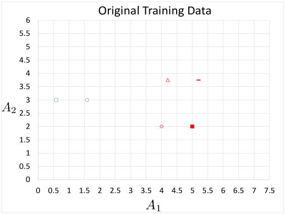
(a) Original Training Data

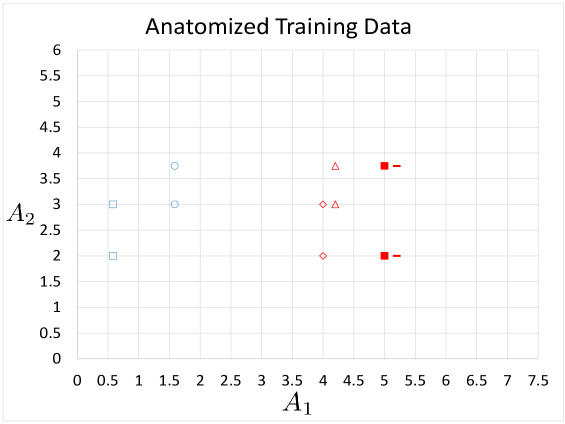
(b) Noisy Training Data ($A_{\_}{id}=A_{\_}1$, $A_{\_}S=A_{\_}2$, $\ell=2$)

Figure 1: Toy Example of Training Data with Two Attributes $A_{\_}1$ and $A_{\_}2$

.

The linear classifier $f$ is an empirical risk minimizer such that $\widehat{f}_{\_}{N}=\underset{f\in\mathcal{F}}{argmin}\widehat{R}_{\_}{N}(f)$. Given the empirical risk minimizer $\widehat{f}_{\_}N$ is the SVC with the largest margin, bound (3.4) holds

(3.4) $$E[R(\widehat{f}_{\_}N)]\leq\frac{E[(R||w||)^{2}]}{N}$$

when the training data is linearly separable [5]. In (3.4), $R$ stands for the radius of the sphere that the shatterable instances lie on and $w$ stands for the weight vector of hyperplane $f(\mathbf{X})$ in (3.1). For the same SVC, the generalization ability is defined in (3.5) according to VC theory [29, 5].

(3.5) $$E[R(\widehat{f}_{\_}N)]-\underset{f\in\mathcal{F}}{inf}R(f)\leq 4\sqrt{\frac{(d+2)log(N+1)+log2}{N}}$$

In (3.5), $\underset{f\in\mathcal{F}}{inf}R(f)$ is the minimum possible risk for the SVC $f$. Next, we define our pruning mechanism for the anatomization.

4 Pruning Mechanism for Anatomization

4.1 Algorithm

We will explain our algorithm ($\sigma_{\_}G$ in Definition 13) through the example in Figure 1(b). The curious reader should visit Figures B.1 and B.2 in the appendix to see the pseudo code and the complexity. Although the example is for any linear classifier (hyperplane), the pruning mechanism is valid for SVC and SVM. We later define the generalization ability of pruned SVC/SVM (cf. Definition 15).

Figure 1(a) shows the original training data with six instances: two instances of a blue class (on the left side) and four of a red class (on the right side), with two attributes $A_{\_}1$ and $A_{\_}2$. Here, every instance has a different shape and filling combination since they are unique. Figure 1(b) shows the anatomized training data with 12 instances created from pairs $IT(A_{\_}1,GID)$ and $ST(GID,A_{\_}2)$ when $\ell=2$ (cf. Definitions 10 and 11).

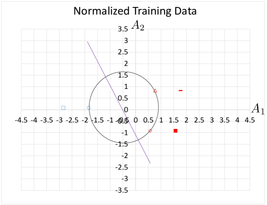
Figure 2: Linear Classifier from Original Training Data

A typical training procedure would be the subtraction of mean from attributes $A_{\_}1$ and $A_{\_}2$ in the original training data, and solving an objective function of a perceptron or SVC (cf. Figure 2). In Figure 2, the original training data is linearly separable and the instances which are closest to the separating hyperplane lie on the surface of the circle . This circle is the key point of linear classification, because the original training data is guaranteed to be linearly separable if the instances that are closest to the decision boundary lie on the surface of a circle [5]. This observation let us define two steps of the pruning mechanism algorithm:

1. Prerequisite Step: Estimate the circle of shatterable instances from the anatomized training data (Algorithm in Figure B.1).

2. Pruning Step: For every group in the anatomized training data, pick an instance that is closest to the surface of the estimated circle of shatterable instances (Algorithm in Figure B.2).

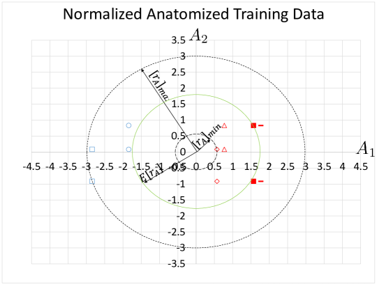
Figure 3: Possible Circles of Shatterable Points

Figure 3 show the range of radiuses for all possible circles of shatterable instances in the prerequisite step. The radius of the original training data must be between the norms of the pair of instances that are closest to (${r_{\_}A}_{\_}{min}$ in Figure 3) and farthest from (${r_{\_}A}_{\_}{max}$ in Figure 3), the origin. Under the random worlds assumption [33], the prerequisite step assumes that $({r_{\_}A}_{\_}{min},{r_{\_}A}_{\_}{max})$ has uniform distribution and therefore estimates the expected radius $E[r]$ with $\frac{{r_{\_}A}_{\_}{min}+{r_{\_}A}_{\_}{max}}{2}$ (dashed green line in Figure 3).

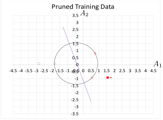
Figure 4: Linear Classifier from Pruned Training Data

Using the estimated radius from the prerequisite step, the pruning step creates the pruned training data in Figure 4. Figure 4 also has the hyperplane that is trained from the pruned training data. Although the shatterable instances of the pruned training data (cf. Figure 4) are the same as the shatterable instances of the original training data (cf. Figure 2), other instances are different. The purpose of the pruning step is to find a linearly separable case instead of distribution reconstruction.

There are two remaining issues to address. First is the application of the pruning algorithm even if the anatomized training data is linearly separable (cf. Figure 1(b)). Even though the anatomized training data is linearly separable in this case, it is not always guaranteed. The instances within each group are not linearly independent from the other $\ell-1$ instances and the shattering property is damaged [5]. The second issue is non-separable original and anatomized training data. If the training data is not linearly separable in the original $(d+1)$ dimensional space, the right approach would be projecting it into higher dimensional space, apply the pruning algorithm in the projected space and hope for the best with a soft margin classifier.

4.2 Privacy Preservation

The preprocessing and pruning steps preserve the $\ell$-diversity condition of anatomization. The algorithm doesn’t estimate the correct matchings between the identifying and the sensitive tables. Instead, it makes a random guess within each group which is expected to give some linearly separable training data. It is possible that the original training data isn’t linearly separable or even is a random set of instances without any pattern (see Section 5).

4.3 Generalization Error of Pruned SVC

We will now give the upper bound on the generalization error of the pruned SVC (cf. Definition 15).

Theorem 4.1

Let $N$ be the number of instances, $d$ be the number of identifying attributes and $d+1$ be the total number of attributes in the original and the pruned training data. Let $R$ be the radius of sphere containing the shatterable instances of the original training data $D$ and $w$ be the weights of the linear hyperplane resulting from linear SV classifier trained on the original training data $D$. Let $R_{\_}p$ and $w_{\_}p$ be the symmetric notations for a linear SV classifier trained on the pruned training data $D_{\_}p$. Assume that all the training instances are located in an Euclidean space $\mathbb{R}^{d+1}$. Let $||*||$ be the Euclidean norm of vector $*$. Let $r^{2}$ be $(R||w||)^{2}$, $r_{\_}p^{2}$ be $(R_{\_}P||w_{\_}p||)^{2}$, $[r_{\_}p^{2}]_{\_}{min}$ be $min\{r_{\_}p^{2}\}>0$ and $[r_{\_}p^{2}]_{\_}{max}$ be $max\{r_{\_}p^{2}\}<\infty$. Let $\widehat{R}_{\_}{N}(f)$ be the empirical risk of on the original training data $D$ and $\widehat{R}_{\_}{N_{\_}p}(f)$ be the empirical risk on the pruned training data. Let $\mathcal{F}$ be the functional space defining the set of possible linear SV classifiers on the original training data $D$ and $\mathcal{F}_{\_}p$ be the functional space of possible linear SV classifiers on the pruned training data $D_{\_}P$. Let $\widehat{f}_{\_}{N}$ be the empirical risk minimizer such that $\widehat{f}_{\_}{N}=\underset{f\in\mathcal{F}}{argmin}\widehat{R}_{\_}{N}(f)$ and $\widehat{f}_{\_}{N_{\_}p}$ be the empirical risk minimizer such that $\widehat{f}_{\_}{N_{\_}p}=\underset{f\in\mathcal{F}_{\_}p}{argmin}\widehat{R}_{\_}{N_{\_}p}(f)$ Last, let $\underset{f\in\mathcal{F}}{inf}R(f)$ be the lowest value of the risk of the linear SV classifier $f$ that could be analytically calculated. Then, the expected risk $E[R(\widehat{f}_{\_}{N_{\_}p})]$ of $\widehat{f}_{\_}{N_{\_}p}$ converges to $\underset{f\in\mathcal{F}}{inf}R(f)$ under the upper bound

(4.6) $$\begin{split}E[R(\widehat{f}_{\_}{N_{\_}p})]-\underset{f\in\mathcal{F}}{inf}R(f)\leq 4&\sqrt{\frac{(d+2)log(N+1)+log2}{N}}\\ &+\frac{[r_{\_}p^{2}]_{\_}{max}-[r_{\_}p^{2}]_{\_}{min}}{N}\end{split}$$

using only $D_{\_}P$.

The proof of Theorem 4.1 is provided in Appendix Section A. The upper bound (4.6) is defined as the function of two terms where the second term is the result of using pruned training data. The former upper bound shows that pruned SVC can be as accurate as the original SVC under two conditions: 1) Very large training data size ($N\to\infty$) 2) Small size of sensitive attribute domain or low $\ell$ value or both ($[r_{\_}p^{2}]_{\_}{max}-[r_{\_}p^{2}]_{\_}{min}\to 0$).

Theorem 4.1 holds when the pruned training data is mapped into a higher dimensional space $d^{\prime}$ using kernel trick. Although the generalization ability of SVMs with RBF kernel is not formally defined (invalid Theorem 4.1), SVMs with RBF kernel are expected to work under the conditions of Theorem 4.1 in the infinite dimensional space [29, 5].

5 Experiments

5.1 Prerequisites

5.1.1 Datasets

We tested our algorithm on the adult, IPUMS and marketing datasets of the UCI data repository [4] and the fatality dataset of Keel data repository [3]:

1. Adult: Adult dataset is drawn from 1994 census data of the United States [4]. It is composed of 45222 instances after the removal of instances with missing values. The binary classification task is to predict whether a person’s adjusted gross income is $\leq 50K$ or $>50K$. The attribute “final weight” is ignored. Last, education was treated as sensitive attribute in the experiments.

2. IPUMS: This data is drawn from the 1970, 1980 and 1990 census data of the Los Angeles and Long Beach areas [4]. It has 233584 instances in total. We picked the 10 attributes that are included in the adult data. The binary classification task is to predict whether a person’s total income is $\leq 50K$ or $>50K$. The classifiers are expected to show a different behavior from the former adult data since the population (and to some extent, classification task, as it is total income rather than adjusted gross income) are different. Last, education was treated as sensitive attribute in the experiments.

   

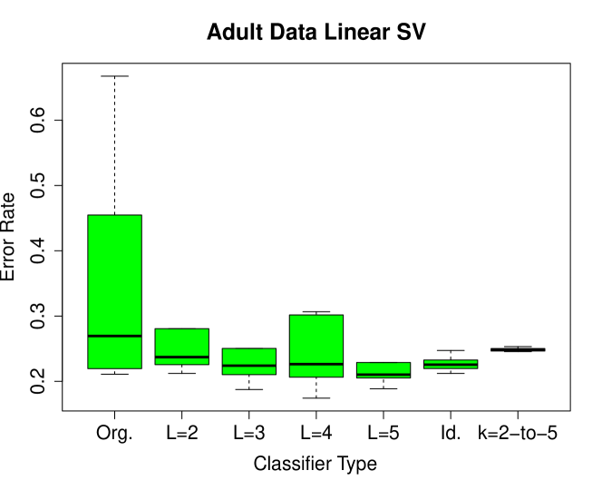
   Figure 5: SVC on Adult

   

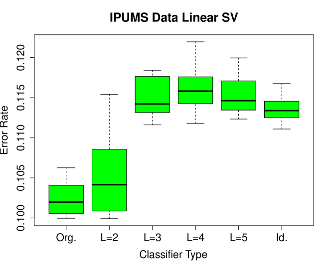
   Figure 6: SVC on IPUMS

The additional information is provided in the appendix for marketing and fatality datasets. Weka was used for attribute selection and discretization if needed [30].

5.1.2 Privacy Setup

The anatomization was done according to Xiao et al.’s bucketization algorithm [33]. When $\ell$-diversity condition is not satisfied, the instances were divided into groups of size $\ell$ according to the original bucketization algorithm. Leftover instances were suppressed (not used in training models).

Anonymized training data was created for the adult dataset. We used Inan et al.’s value generalization hierarchies in the experiments. The privacy parameters were $k=\ell$ for $k$-anonymity and $\ell$-diversity to compare the classifiers using same group sizes in training data.

Anonymized and anatomized training data had the same identifying and sensitive attributes. The sensitive attributes were chosen such that the $\ell$-diversity is satisfied for at least $\ell=2$.

5.1.3 Model Evaluation Setup

LibSVM version 3.21 was used for the support vector classification [6]. We will train the support vector machine with linear (SVC) and RBF kernels (SVM).

10-fold cross validation was used for evaluation. The comparison includes pruned SVC/SVM, original SVC/SVM and identifying SVC/SVM. The comparison on adult dataset also include anonymized SVC/SVM. The anonymized SVC/SVM are not included for other datasets since Inan et al. provided generalization hierarchies only in the adult dataset [15]. Last, the error rates of pruned and original SVC/SVM are compared using the Student $t$-test (See Appendix). Other models are not included, because Theorem 4.1 covers only pruned and original SVC/SVM.

5.2 Analysis of Results

Figures 5, 6 (see above) and C.1 through C.8 (see Appendix) show the boxplots of error rates for SVC and SVM. In all Figures, “Org.” and “Id.” labels will stand for original SVC/SVM and identifying SVC/SVM respectively. The pruned and anonymized SVC/SVM will be represented by their respective privacy parameters (L for $\ell$ and k for $k$.) This section will include the discussion of results in Figures 5 and 6. (See Appendix for analysis of other results.) The analysis have three observation aspects.

The first is the comparison between the pruned and the original SVC/SVM. From Theorem 4.1, we expect that the average error rate of the pruned SVC/SVM will be higher than the average error rate of the original SVC/SVM because bound (4.6) has the additional second term at the right-hand side (cf. Section 4.3). Increasing the $\ell$ parameter would result in the increase of the average error rate if the training data size remains same between multiple $\ell$ values (no suppression). The rate of the error rate increase in function of $\ell$ is theoretically hard to estimate since the assignments of sensitive attributes to each group will be random throughout the bucketization algorithm [33]. Figure 6 show the expected behaviour for the pruned SVC. The average error rates in Figure 5 show a surprising result. We observe that the pruned SVC outperforms the original SVC for multiple $\ell$ values. Moreover, the average error rate decreases when $\ell$ is increased. Here, the assumption of Theorem 4.1 is violated because of suppression for $\ell\geq 4$. The bound 4.6 thus does not hold and the result is statistically insignificant (see Appendix.)

The second aspect is the comparison between pruned and identifying SVC/SVM. In the first case, the identifying SVC/SVM are likely to outperform the pruned SVC/SVM if the sensitive attribute is a bad predictor of the class attribute in the original training data. The sensitive attribute damages the shattering property of the instances in the original training data and the instances near the decision boundary are not on the surface of a sphere. The pruned SVC/SVM estimates a model of the original training data that is not likely to generalize well. Figure 5 shows a bad predictor case, because the average error rates of the identifying SVC is less than the average error rates of the pruned SVC when $\ell$ is 2 to 4. $\ell=5$ is a special case where the pruning algorithm and $\ell$-diversity show the regularization effect to reduce the bias of the underfitting original SVC. In the second case, the pruned SVC/SVM are likely to outperform the identifying SVC/SVM if the sensitive attribute is a good predictor of the class attribute in the original training data. The symmetric shattering argument implicitly holds here. Figure 6 shows a special case of a good predictor. The pruned SVC outperforms the identifying SVC only for $\ell=2$. For $\ell$ values 3 to 5, the pruning algorithm and $\ell$-diversity act like a poorly tuned regularizer that cause overfitting. Unfortunately, we cannot know whether the sensitive attribute is a good or bad predictor. Knowing such a behavior would indicate the prediction of the sensitive attribute, a defacto violation of $\ell$-diversity.

The third aspect is the comparison between the pruned and the anonymized SVC/SVM. Figure 5 show the anonymized SVC/SVM in addition to the anatomized and original SVC/SVM. The anatomized SVC/SVM are expected to outperform the anonymized SVC/SVM because anatomization preserves the original values for all the attributes. The generalization based $k$-anonymity, on the other hand, distorts most of the original attribute values [15]. In Figure 5, the average error rate of the pruned SVC is less than the anonymized SVC’s when $\ell$ is 3 to 5. These results show the advantage of anatomization versus generalization-based $k$-anonymity. Anatomization has high data utility while the sensitive attribute has a strong privacy guarantee, unlike generalization-based $k$-anonymity.

6 Conclusion and Future Directions

We proposed a preprocessing algorithm for anatomization. Our algorithm estimates a linearly separable training data from the anatomized training data. We defined the generalization ability of support vector classifiers when they are trained on the former preprocessed data. The key point to remember is that our algorithm gives good generalization guarantees to support vector classifiers. The proposed mechanism is evaluated on multiple publicly available datasets and accurate models were observed in most cases while $\ell$-diversity is preserved.

There are multiple future directions for this work. First is the development of other classification or clustering algorithms for anatomization. Second is the extension of current work to the $k$-anonymity or generalization based $\ell$-diversity. Considering multiple sensitive attributes is also another direction.

See pages - of appendix

References

- [1] D. Agrawal and C. C. Aggarwal, On the design and quantification of privacy preserving data mining algorithms, in Proceedings of the Twentieth ACM SIGACT-SIGMOD-SIGART Symposium on Principles of Database Systems, Santa Barbara, California, May 21-23 2001, ACM, pp. 247–255.
- [2] R. Agrawal and R. Srikant, Privacy-preserving data mining, in Proceedings of the 2000 ACM SIGMOD Conference on Management of Data, Dallas, TX, May 14-19 2000, ACM, pp. 439–450.
- [3] J. Alcalá, A. Fernández, J. Luengo, J. Derrac, S. García, L. Sánchez, and F. Herrera, Keel data-mining software tool: Data set repository, integration of algorithms and experimental analysis framework, Journal of Multiple-Valued Logic and Soft Computing, 17 (2010), p. 11.
- [4] A. Asuncion and D. Newman, UCI machine learning repository, 2007.
- [5] C. J. Burges, A tutorial on support vector machines for pattern recognition, vol. 2, January 1998, pp. 121–167.
- [6] C.-C. Chang and C.-J. Lin, Libsvm: a library for support vector machines, ACM Transactions on Intelligent Systems and Technology (TIST), 2 (2011), p. 27.
- [7] V. Ciriani, S. D. C. D. Vimercati, S. Foresti, S. Jajodia, S. Paraboschi, and P. Samarati, Combining fragmentation and encryption to protect privacy in data storage, ACM Trans. Inf. Syst. Secur., 13 (2010), pp. 22:1–22:33.
- [8] G. Cormode, N. Li, T. Li, and D. Srivastava, Minimizing minimality and maximizing utility: Analyzing method-based attacks on anonymized data, in Proceedings of the VLDB Endowment, vol. 3, 2010, pp. 1045–1056.
- [9] S. D. C. di Vimercati, S. Foresti, S. Jajodia, G. Livraga, S. Paraboschi, and P. Samarati, Extending loose associations to multiple fragments, in DBSec’13, 2013, pp. 1–16.
- [10] J. Dowd, S. Xu, and W. Zhang, Privacy-preserving decision tree mining based on random substitutions, tech. report, In International Conference on Emerging Trends in Information and Communication Security, 2005.
- [11] C. Dwork, Differential privacy, in 33rd International Colloquium on Automata, Languages and Programming (ICALP 2006), Venice, Italy, July 9-16 2006, pp. 1–12.
- [12] A. Evfimievski, J. Gehrke, and R. Srikant, Limiting privacy breaches in privacy preserving data mining, in Proceedings of the 22nd ACM SIGACT-SIGMOD-SIGART Symposium on Principles of Database Systems (PODS 2003), San Diego, CA, June 9-12 2003, pp. 211–222.
- [13] T. Gal, Z. Chen, and A. Gangopadhyay, A privacy protection model for patient data with multiple sensitive attributes, International Journal of Information Security and Privacy, IGI Global, Hershey, PA, 2 (2008), pp. 28–44.
- [14] X. He, Y. Xiao, Y. Li, Q. Wang, W. Wang, and B. Shi, Permutation anonymization: Improving anatomy for privacy preservation in data publication., in PAKDD Workshops, L. Cao, J. Z. Huang, J. Bailey, Y. S. Koh, and J. Luo, eds., vol. 7104 of Lecture Notes in Computer Science, Springer, 2011, pp. 111–123.
- [15] A. Inan, M. Kantarcioglu, and E. Bertino, Using anonymized data for classification, in Proceedings of the 2009 IEEE International Conference on Data Engineering, ICDE ’09, Washington, DC, USA, 2009, IEEE Computer Society, pp. 429–440.
- [16] V. Iyengar, Transforming data to satisfy privacy constraints, in Proc., the Eigth ACM SIGKDD Int’l Conf. on Knowledge Discovery and Data Mining, 2002, pp. 279–288.
- [17] P. Jain and A. Thakurta, Differentially private learning with kernels., ICML (3), 28 (2013), pp. 118–126.
- [18] D. Kifer, Attacks on privacy and de finetti’s theorem, in In SIGMOD, 2009.
- [19] N. Li and T. Li, t-closeness: Privacy beyond k-anonymity and l-diversity, in Proceedings of the 23nd International Conference on Data Engineering (ICDE ’07), Istanbul, Turkey, Apr. 16-20 2007.
- [20] T. Li and N. Li, On the tradeoff between privacy and utility in data publishing, in Proceedings of the 15th ACM SIGKDD International Conference on Knowledge Discovery and Data Mining, Paris, France, June 28 - July 1, 2009, 2009, pp. 517–526.
- [21] T. Li, N. Li, J. Zhang, and I. Molloy, Slicing: A new approach for privacy preserving data publishing, IEEE Trans. Knowl. Data Eng., 24 (2012), pp. 561–574.
- [22] K.-P. Lin and M.-S. Chen, Privacy-preserving outsourcing support vector machines with random transformation, in Proceedings of the 16th ACM SIGKDD International Conference on Knowledge Discovery and Data Mining, KDD ’10, New York, NY, USA, 2010, ACM, pp. 363–372.
- [23] A. Machanavajjhala, J. Gehrke, D. Kifer, and M. Venkitasubramaniam, -diversity: Privacy beyond -anonymity, in Proceedings of the 22nd IEEE International Conference on Data Engineering (ICDE 2006), Atlanta Georgia, Apr. 2006.
- [24] R. A. Moore, Jr., Controlled data-swapping techniques for masking public use microdata sets, Statistical Research Division Report Series RR 96-04, U.S. Bureau of the Census, Washington, DC., 1996.
- [25] M. E. Nergiz and C. Clifton, -presence without complete world knowledge, 22 (2010), pp. 868–883.
- [26] B. I. Rubinstein, P. L. Bartlett, L. Huang, and N. Taft, Learning in a large function space: Privacy-preserving mechanisms for svm learning, arXiv preprint arXiv:0911.5708, (2009).
- [27] P. Samarati, Protecting respondent’s privacy in microdata release, 13 (2001), pp. 1010–1027.
- [28] L. Sweeney, k-anonymity: a model for protecting privacy, International Journal on Uncertainty, Fuzziness and Knowledge-based Systems, (2002), pp. 557–570.
- [29] V. N. Vapnik and V. Vapnik, Statistical learning theory, vol. 1, Wiley New York, 1998.
- [30] I. H. Witten and E. Frank, Data Mining: Practical Machine Learning Tools and Techniques with Java Implementations, Morgan Kaufmann, San Francisco, Oct. 1999.
- [31] R. C.-W. Wong, A. W.-C. Fu, K. Wang, and J. Pei, Minimality attack in privacy preserving data publishing, in VLDB, 2007, pp. 543–554.
- [32] R. C.-W. Wong, J. Li, A. W.-C. Fu, and K. Wang, (, k)-anonymity: An enhanced k-anonymity model for privacy preserving data publishing, in Proceedings of the 12th ACM SIGKDD International Conference on Knowledge Discovery and Data Mining, KDD ’06, New York, NY, USA, 2006, ACM, pp. 754–759.
- [33] X. Xiao and Y. Tao, Anatomy: Simple and effective privacy preservation, in Proceedings of 32nd International Conference on Very Large Data Bases (VLDB 2006), Seoul, Korea, Sept. 12-15 2006.