Nonstationary POT modelling of air pollution concentrations: Statistical analysis of the traffic and meteorological impact

Abstract

Predicting the occurrence, level and duration of high air pollution concentrations exceeding a given critical level enables researchers to study the health impact of road traffic on local air quality and to inform public policy action. Precise estimates of the probabilities of occurrence and level of extreme concentrations are formidable due to the combination of complex physical and chemical processes involved. This underpins the need for developing sophisticated extreme value models, in particular allowing for non-stationarity of environmental time series. In this paper, extremes of nitrogen oxide (NO), nitrogen dioxide ($\text{NO}_{2}$) and ozone ($\text{O}_{3}$) concentrations are investigated using two models. Model I is based on an extended peaks-over-threshold (POT) approach developed by A. C. Davison and R. L. Smith, whereby the parameters of the underlying generalized Pareto distribution (GPD) are treated as functions of covariates (i.e., traffic and meteorological factors). The new Model II resolves the lack of threshold stability in the Davison–Smith model by constructing a special functional form for the GPD parameters. For each of the models, the effects of traffic and meteorological factors on the frequency and size of extreme values are estimated using Markov chain Monte Carlo methods. Finally, appropriate goodness-of-fit tests and model selection criteria confirm that Model II significantly outperforms Model I in estimation and forecasting of extremes.

Keywords: Roadside air pollution; Extreme values; Peaks-over-threshold (POT); Generalized Pareto distribution (GPD); Non-stationarity; Threshold stability.

2010 MSC: Primary: 62G32; Secondary: 60G70, 62F15, 62G05.

1 Introduction

The issue of high episodic concentrations of air pollutants (e.g., nitrogen oxides, particulates, and carbon monoxide) is a matter of growing worldwide concern due to their harmful effects on human health and the environment. Among many contributing factors, road traffic emission is accounted for high proportions of harmful pollutants. Accurate prediction of pollution episodes, including their magnitude and duration, is a formidable problem due to the combination of many complex physical and chemical processes involved in their formation. Hence, there is a need for the development of sophisticated extreme value models in order to facilitate prediction of high pollution concentrations and to better understand their cause.

Statistical analysis of air pollution data has been extensively advanced in the recent decade (see, e.g., Carslaw et al., 2007; Zito et al., 2008; and references therein). In general, research in this area aims to pursue the following long-term goals (Thompson et al., 2001; Eastoe & Tawn, 2009):

• predicting critical levels of pollutants to give out health warnings to public;

• identifying and predicting trends in high concentration levels;

• assessing changes in air pollution levels due to the impact of human activities on the environment, either direct (e.g., via changing emission patterns) or indirect (through the climate change).

As argued by Eastoe and Tawn (2009), statistical methodology based on extreme value theory is particularly suited to address these problems. An extensive discussion of extreme value methods useful in the air quality modelling can also be found in Horowitz and Barakat (1979), Smith (1989), and Küchenhoff and Thamerus (1996).

In the present paper, a novel approach to extreme value modelling is proposed, tailored to the problems indicated above on both long (e.g., daily or yearly) and short (e.g., 15 min) time scales. The latter is particularly important in environmental and health applications due to the fact that even a short exposure to high pollution concentrations may have harmful effects on human health, for example, asthmatic patients exposed to a high sulphur dioxide ($\text{SO}_{2}$) concentration may develop adverse symptoms within minutes (WHO, 2000).

The models presented in this paper are used to analyse the nitrogen oxide (NO), nitrogen dioxide ($\text{NO}_{2}$), collectively referred to as $\text{NO}_{x}$, and ozone ($\text{O}_{3}$) concentration data (see Figure 1), which consist of $15$-min maxima of $1$-min concentration values observed within one calendar year, from January 1, 2008 to January 1, 2009. The data were collected at a fixed roadside laboratory on Kirkstall Road in the city of Leeds (West Yorkshire, UK). The laboratory houses a traffic monitoring system and an air quality monitoring station, in which local meteorological conditions are recorded (see more details in Section 3.5).

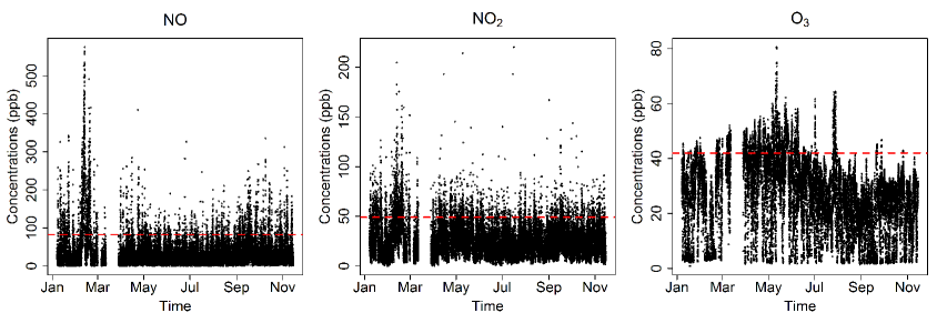
Figure 1: Time-series plots of 15-min maximum concentrations of $\text{NO}_{x}$ and $\text{O}_{3}$ (expressed in ppb = parts-per-billion), collected at the Kirkstall roadside laboratory from 1 January 2008 till 1 January 2009. Missing data are left blank. The empirical $90\%$-quantiles of the concentration values are indicated by the dashed lines (red in the online version).

As demonstrated in Figure 1, all three chemicals have a highly variable dynamic behaviour, with noticeable evidence of nonstationarity. Temporal variation in the mean and variance, as well as in the patterns of extreme values, can be explained by the underlying physical and chemical processes. An additional remarkable feature of these plots is that the three chemicals are apparently strongly correlated, which can be attributed to the photochemical interconversion reactions between the pollutants (Clapp & Jenkin, 2001). Despite a large number of chemical processes potentially oxidizing NO and $\text{NO}_{2}$, the most important source of secondary $\text{NO}_{2}$ is the following reaction:

$$\text{NO}+\text{O}_{3}\to\text{NO}_{2}+\text{O}_{2},\qquad\text{NO}_{2}+h\nu\,(+\text{O}_{2})\to\text{NO}+\text{O}_{3}.$$ (1)

Due to the asymmetry of the reactions (1), the equilibrium concentration levels (photostationary state) strongly depend on the presence (or otherwise) of sunlight ($h\nu$), in particular leading to decreased levels of $\text{NO}_{x}$ (and, correspondingly, increased levels of ozone $\text{O}_{3}$) during the summer due to a higher solar radiation. Hence, there are yearly cycles in the time series of concentrations. There is also a difference between daylight and night-time measurements that can be explained by the lack of sunshine at night and dry deposition in the early morning. In addition, the emission of $\text{NO}_{x}$ also follows some daily, weekly and seasonal trends, which are due to the traffic patterns (including peak hours and weekday–weekend oscillations) and to the seasonal variability of human activities, such as emission from plants and motor vehicles, combustion of fossil fuels in habitations, etc. Specifically, the data under study correspond to traffic-dominated emission sources.

In the present work, the extreme value models are developed furnishing an efficient tool to estimate the probabilities of future extreme events, conditional on the traffic and meteorological covariates. In particular, these models account for nonstationarity of pollution concentrations; thus the effects of possible future scenarios relating to changes in emission patterns and climate can also be quantified. Despite the apparently high correlation between the three pollutants under study, in this work we confine ourselves to univariate models for each chemical, which however prove to be rather efficient (see further comments in Section 5).

2 Peaks-over-threshold models

Suppose that observations $X_{1},X_{2}\dots$ are independent and identically distributed (i.i.d.) random variables with a common continuous distribution function $F(x)=\mathsf{P}(X_{t}\leq x)$ ($-\infty<x<\infty$). There are two main approaches in the literature to characterization of extreme values in the sequence $(X_{t})$ (see Smith, 1989, for a review and further bibliography therein). The classic block-maxima method based on the Fisher–Tippett–Gnedenko theorem (see Embrechts et al., 1997) proceeds by picking the maximum values over certain blocks of data of large enough size $n$ (e.g., one year worth of data each) and approximating them via a generalized extreme value (GEV) distribution function,

$$\mathsf{P}\bigl{(}\max\{X_{1},\dots,X_{n}\}\leq x\bigr{)}\approx F_{\mathrm{GEV}}(x;\mu,\sigma,\xi)=\exp\left\{-\left(1+\frac{\xi(x-\mu)}{\sigma}\right)_{+}^{-1/\xi}\right\},$$ (2)

where $a_{+}=\max\{a,0\}$ and $\mu$, $\sigma$ and $\xi$ are the location, scale and shape parameters, respectively. Three distinct subclasses of the GEV family (2) are known as the Fréchet ($\xi>0)$, Weibull ($\xi<0$), and Gumbel ($\xi=0$) distributions (the latter is interpreted as the limit of (2) as $\xi\rightarrow 0$).

A more recent peaks-over-threshold (POT) method (see Embrechts et al., 1997) focuses on exceedances within the original sample $(X_{t})$ over a high threshold $u$, that is, $X_{t}^{u}=X_{t}-u$ conditioned on the event $X_{t}>u$. The phrase “high threshold” means that $u$ is close to the upper boundary of the support of the GEV distribution (2), that is, $u\to\mu+\sigma/(-\xi)$ ($\xi<0$) or $u\to\infty$ ($\xi\geq 0$). In particular, the threshold exceedance rate

$$\rho_{u}=\mathsf{P}(X_{t}>u)$$ (3)

is small. The corresponding approximation, conveniently written for the tail distribution function, is known as the generalized Pareto distribution (GPD),

$$\mathsf{P}(X_{t}^{u}>x)=\mathsf{P}(X_{t}>u+x\,|\,X_{t}>u)\approx\bar{F}_{\mathrm{GPD}}(x;\sigma_{u},\xi)=\left(1+\frac{x\,\xi}{\sigma_{u}}\right)_{+}^{-1/\xi},\qquad x\geq 0,$$ (4)

with the same shape parameter $\xi$ as in (2) (hence, not depending on the threshold value $u$) and a new scale parameter $\sigma_{u}=\sigma+\xi(u-\mu)$. The GPD approximation (4) holds whenever the GEV approximation (2) does (Pickands, 1975). Note that for $\xi\geq 0$ the support of the GPD (4) is the half-line $[0,\infty)$, whereas for $\xi<0$ it is a bounded interval, $0\leq x\leq\sigma_{u}/(-\xi)$.

Because the air quality standards and objectives are normally expressed in terms of certain critical thresholds, the POT approach is apparently more suitable and better interpretable in the air pollution context. Moreover, there is a growing recognition among statisticians and environmental modellers that the POT is superior to the block-maxima approach in that the latter ignores any secondary extreme values in each block (i.e., next to the largest one) and thus leads to loss of information; consequently, the POT has a strong potential to provide an improved accuracy of estimation and inference (Coles, 2001).

In the influential paper of Davison and Smith (1990), an extension of the POT method to the nonstationary case was proposed, based on treating the parameters of the GPD as functions of covariates. This method was applied in the air pollution context, for example, by Eastoe and Tawn (2009), to model the extremes of surface level ozone ($\text{O}_{3}$) concentrations.

In the present paper, our first goal is to build a dynamic version of the Davison–Smith model (referred to as Model I) to estimate the distribution of extreme concentration values (threshold exceedances) in terms of the traffic and meteorological conditions and also to assess the impact of these covariates on the extremes. Furthermore, we propose a special functional form for the parameters of the GPD (leading to the new Model II) to ensure consistency over different threshold choices. This resolves the intrinsic problem of threshold stability of the GPD in the nonstationary case (cf. Eastoe & Tawn, 2009; Northrop et al., 2016); to the best of our knowledge, such a solution is new. Due to analytical and computational complexities, estimation of the model parameters and variable selection in both Models I and II were carried out within the Bayesian framework by using a suitable Markov Chain Monte Carlo (MCMC) procedure (Gilks et al., 1996).

The rest of the paper is organized as follows. The methodology based on an extension of the Davison–Smith model is set out in Section 3. The results of the model fitting are presented in Section 4 along with the estimation of extreme events. This is followed in Section 5 by a discussion of the inference obtained.

3 Methodology

3.1 GPD model with covariates

Let us introduce the necessary notation and describe our models in more detail. Let $(X_{t})$ be a (discrete-time) random process representing the temporal dynamics of the concentration of a specific pollutant, and let $u$ be a selected (high) threshold level. If the observed values $(X_{t})$ are i.i.d. and a GEV approximation (2) holds, then the (conditional) distribution function of the threshold exceedances $X_{t}^{u}=X_{t}-u$ can be approximated by the GPD (see (4)).

Following Davison and Smith (1990), nonstationarity of observations $(X_{t})$ (and hence of the threshold exceedances) is incorporated in Model I through the conditional distribution

$$\mathsf{P}(X^{u}_{t}>x\,|\,\boldsymbol{C}_{t}=\boldsymbol{c})=\mathsf{P}(X_{t}>u+x\,|\,X_{t}>u,\,\boldsymbol{C}_{t}=\boldsymbol{c}),\qquad x\geq 0,$$ (5)

where $\boldsymbol{C}_{t}$ denotes the random vector of relevant covariates at time $t$ (such as traffic and meteorological conditions), with values $\boldsymbol{c}$ in a suitable covariate space $\mathcal{C}$. Full details of the covariates used in the model building are described in Section 3.5. The marginal distribution of the exceedances $X_{t}^{u}$ is obtained by integrating over the covariates,

$$\mathsf{P}(X^{u}_{t}>x)=\int_{\mathcal{C}}\mathsf{P}\left(X^{u}_{t}>x\,|\,\boldsymbol{C}_{t}=\boldsymbol{c}\right)f_{t}(\boldsymbol{c})\,\mathrm{d}\boldsymbol{c},\qquad x\geq 0,$$ (6)

where $f_{t}(\boldsymbol{c})$ is the density of $\boldsymbol{C}_{t}$. In practice, the function $f_{t}(\boldsymbol{c})$ is not known but can be estimated by its empirical version using a subset of observation times where the covariate vector takes values close to a given $\boldsymbol{c}\in\mathcal{C}$.

The statistical analysis is greatly simplified under the standard assumption that the conditional distribution (5) does not depend on time $t$. That is to say, the covariate vector $\boldsymbol{C}_{t}$ plays a role of a sufficient statistic incorporating all information contained in the data about nonstationarity of the threshold exceedances. This assumption is in fact the backbone of the Davison–Smith modelling approach.

As a result, the GPD approximation (4) takes the form

$$\mathsf{P}(X^{u}_{t}>x\,|\,\boldsymbol{C}_{t}=\boldsymbol{c})\approx\bar{F}_{\mathrm{GPD}}\left(x;\sigma_{u}(\boldsymbol{c}),\xi(\boldsymbol{c})\right)=\left(1+\frac{x\,\xi(\boldsymbol{c})}{\sigma_{u}(\boldsymbol{c})}\right)_{+}^{-1/\xi(\boldsymbol{c})},\qquad x\geq 0,$$ (7)

where the GPD parameters $\sigma_{u}=\sigma_{u}(\boldsymbol{c})$ and $\xi=\xi(\boldsymbol{c})$ are functions of the current value of the covariate vector $\boldsymbol{C}_{t}=\boldsymbol{c}$.

Likewise, the rate of threshold exceedance at time $t$ (see (3)) should also be interpreted as a covariate-dependent quantity,

$$\rho_{u}(\boldsymbol{c})=\mathsf{P}(X_{t}>u\,|\,\boldsymbol{C}_{t}=\boldsymbol{c}).$$ (8)

Note that the probability of the event $X_{t}>u+x$ conditioned on the covariates (i.e., the exceedance rate for a higher threshold $u+x$) is given by

$$\rho_{u+x}(\boldsymbol{c}) =\mathsf{P}(X_{t}>u+x\,|\,\boldsymbol{C}_{t}=\boldsymbol{c})$$

$$=\mathsf{P}(X_{t}>u\,|\,\boldsymbol{C}_{t}=\boldsymbol{c})\cdot\mathsf{P}(X_{t}>u+x\,|\,X_{t}>u,\,\boldsymbol{C}_{t}=\boldsymbol{c})$$

$$=\rho_{u}(\boldsymbol{c})\cdot\mathsf{P}(X^{u}_{t}>x\,|\,\boldsymbol{C}_{t}=\boldsymbol{c})$$

$$\approx\rho_{u}(\boldsymbol{c})\left(1+\frac{x\,\xi(\boldsymbol{c})}{\sigma_{u}(\boldsymbol{c})}\right)_{+}^{-1/\xi(\boldsymbol{c})},$$ (9)

according to GPD (7).

Let us now introduce the usual regression-type parametric assumption (cf. Davison & Smith, 1990; Eastoe, 2009; Eastoe & Tawn, 2009) for the functional link between the model parameters and the covariates. To be specific, suppose that the covariate vector $\boldsymbol{c}$ is $m$-dimensional (including any dummy variables if required) and, without loss of generality, $\boldsymbol{c}\in\mathbb{R}^{m}$. In order to accommodate baseline effects (intercepts) in our regression models, it is also convenient to introduce the extended covariate vector

$$\tilde{\boldsymbol{c}}^{\top}=(1,c_{1},\dots,c_{m})\in\mathbb{R}^{m+1},$$

where $\boldsymbol{x}^{\top}$ denotes the transpose of a (column) vector $\boldsymbol{x}$. In what follows, we use the standard notation

$$\mathop{\mathrm{logit}}\nolimits\rho=\ln\left(\frac{\rho}{1-\rho}\right),\qquad 0<\rho<1.$$

Assumption 1.

The quantities $\ln\sigma_{u}(\boldsymbol{c})$,  $\xi(\boldsymbol{c})$ and $\mathop{\mathrm{logit}}\nolimits\rho_{u}(\boldsymbol{c})$ are linear functions of the covariates,

$$\ln\sigma_{u}(\boldsymbol{c})=\boldsymbol{s}_{u}^{\top}\mbox{$\>\!$}\tilde{\boldsymbol{c}},\ \ \quad\xi(\boldsymbol{c})=\boldsymbol{\kappa}^{\top}\tilde{\boldsymbol{c}},\ \ \quad\mathop{\mathrm{logit}}\nolimits\rho_{u}(\boldsymbol{c})=\boldsymbol{r}_{u}^{\top}\mbox{$\>\!$}\tilde{\boldsymbol{c}},$$ (10)

where $\boldsymbol{s}_{u}$, $\boldsymbol{\kappa}$ and $\boldsymbol{r}_{u}$ are the corresponding $(m+1)$-dimensional vector coefficients (effects).

The regression setting (10) is the basis of our Model I.

3.2 Threshold stability

The desirable property of the GPD is its consistency with regard to the variable choice of the threshold, referred to as the threshold stability: if the conditional distribution of exceedances over $u$ is a GPD with parameters $\sigma_{u}$ and $\xi$, then the conditional distribution of exceedances over a higher level $u+x$ ($x\geq 0$) should also be given by a GPD with the same shape parameter $\xi$ and the new scale parameter $\sigma_{u+x}=\sigma_{u}+x\,\xi$ (Embrechts et al., 1997). In the nonstationary case, this conditions transcribes as

$$\sigma_{u+x}(\boldsymbol{c})=\sigma_{u}(\boldsymbol{c})+x\,\xi(\boldsymbol{c}).$$ (11)

As was pointed out by Eastoe and Tawn (2009), the Davison–Smith model in general does not guarantee the threshold stability: even if $\xi(\boldsymbol{c})$ is constant, $\sigma_{u+x}(\boldsymbol{c})$ must be either constant (leading back to the stationary case) or a linear function, which contradicts the log-linear formulation of the model (10).

We suggest a solution to this problem by using a special functional form for the scale and shape parameters, which then leads to what we call Model II. Observe that, according to (11), $\sigma_{u}(\boldsymbol{c})$ is linear in $u$. Thus, the proposed functional parameterization is as follows:

$$\sigma_{u}(\boldsymbol{c})=\bigl{(}\alpha(\boldsymbol{c})+u\mbox{$\>\!$}\beta(\boldsymbol{c})\bigr{)}\,\mathrm{e}^{\gamma(\boldsymbol{c})},\qquad\xi(\boldsymbol{c})=\beta(\boldsymbol{c})\,\mathrm{e}^{\gamma(\boldsymbol{c})},$$ (12)

where $\alpha(\boldsymbol{c})$, $\beta(\boldsymbol{c})$ and $\gamma(\boldsymbol{c})$ are functions of the covariates, subject to the constraint that $\alpha(\boldsymbol{c})+u\mbox{$\>\!$}\beta(\boldsymbol{c})>0$. It is easy to verify that the formulas (12) secure the threshold stability condition (11):

$$\sigma_{u}(\boldsymbol{c})+x\,\xi(\boldsymbol{c}) =\bigl{(}\alpha(\boldsymbol{c})+u\mbox{$\>\!$}\beta(\boldsymbol{c})\bigr{)}\,\mathrm{e}^{\gamma(\boldsymbol{c})}+x\mbox{$\;\!$}\beta(\boldsymbol{c})\,\mathrm{e}^{\gamma(\boldsymbol{c})}$$

$$=\bigl{(}\alpha(\boldsymbol{c})+(u+x)\mbox{$\;\!$}\beta(\boldsymbol{c})\bigr{)}\,\mathrm{e}^{\gamma(\boldsymbol{c})}=\sigma_{u+x}(\boldsymbol{c}).$$

By analogy with the regression setting (10), it is natural to introduce the following

Assumption 2.

The coefficients $\alpha(\boldsymbol{c})$, $\beta(\boldsymbol{c})$ and $\gamma(\boldsymbol{c})$ of the model (12), as well as $\mathop{\mathrm{logit}}\nolimits\rho_{u}(\boldsymbol{c})$ as before, are linear functions of the covariates,

$$\alpha(\boldsymbol{c})=\boldsymbol{a}^{\top}\tilde{\boldsymbol{c}},\ \ \quad\beta(\boldsymbol{c})=\boldsymbol{b}^{\top}\tilde{\boldsymbol{c}},\ \ \quad\gamma(\boldsymbol{c})=\boldsymbol{g}^{\top}\tilde{\boldsymbol{c}},\ \ \quad\mathop{\mathrm{logit}}\nolimits\rho_{u}(\boldsymbol{c})=\boldsymbol{r}_{u}^{\top}\mbox{$\>\!$}\tilde{\boldsymbol{c}}.$$ (13)

Note that the regression vectors $\boldsymbol{a}$, $\boldsymbol{b}$ and $\boldsymbol{g}$ do not depend on the threshold $u$, in accord with the construction of the threshold-stable Model II. So we need to estimate these coefficients only once, for a suitable level $u$, then they can be used for any level $u+x$. As for the threshold exceedance rate $\rho_{u}$, once it has been estimated at the level $u$ it can be directly calculated for another level $u+x$ using the formula (9).

3.3 Bayesian model estimation with MCMC

Recall that MCMC simulation techniques are based on running a suitable Markov chain whose equilibrium distribution is the desired (posterior) distribution of the model parameters (Gilks et al., 1996). In addition to computational convenience and efficiency, this methodology provides more information as compared to the conventional maximum likelihood inference; for instance, it makes it possible to find the predictive distribution for future extreme events (Beirlant et al., 2004).

Estimation of the parameters in our models was carried out using the Metropolis–Hastings MCMC algorithm (Gilks et al., 1996). The general framework of this algorithm is as follows. Let $\boldsymbol{X}$ be a random sample from the target distribution with density $f(\boldsymbol{x}\mbox{$\>\!$}|\mbox{$\>\!$}\boldsymbol{\theta})$, and let $q(\boldsymbol{\theta})$ be the prior density of the unknown vector parameter $\boldsymbol{\theta}$. The likelihood function is denoted by $L(\boldsymbol{\theta}\mbox{$\>\!$}|\mbox{$\>\!$}\boldsymbol{X})=f(\boldsymbol{X}\mbox{$\>\!$}|\mbox{$\>\!$}\boldsymbol{\theta})$. According to the Bayes theorem, the posterior density $q(\boldsymbol{\theta}\mbox{$\;\!$}|\mbox{$\>\!$}\boldsymbol{X})$ is proportional to $L(\boldsymbol{\theta}\mbox{$\>\!$}|\mbox{$\>\!$}\boldsymbol{X})\,q(\boldsymbol{\theta})$. The aim of the Metropolis–Hastings algorithm is to generate a sample from the posterior distribution $q(\boldsymbol{\theta}\mbox{$\;\!$}|\mbox{$\>\!$}\boldsymbol{X})$ obtained as the equilibrium distribution $\pi(\boldsymbol{\theta})$ of a certain Markov chain $(\boldsymbol{\theta}_{k})$ in the parameter space (whereby the next state $\boldsymbol{\theta}_{k+1}$ depends only on the present state $\boldsymbol{\theta}_{k}$ but not on the past states $\boldsymbol{\theta}_{j}$ with $j<k$). In turn, $\pi(\boldsymbol{\theta})$ can be approximated by a long run of the Markov chain $(\boldsymbol{\theta}_{k})$, which relies on good mixing of the chain and fast enough convergence to the equilibrium. The suitable Markov chain is implemented using a generalized acceptance–rejection sampling method. Namely, at each step, given the current state $\boldsymbol{\theta}$ of the chain a new candidate state $\boldsymbol{\theta}^{\prime}$ is generated according to a proposal density $g(\boldsymbol{\theta}^{\prime}\mbox{$\>\!$}|\mbox{$\;\!$}\boldsymbol{\theta})$, which is accepted with probability

$$A(\boldsymbol{\theta}^{\prime}\mbox{$\>\!$}|\mbox{$\;\!$}\boldsymbol{\theta})=\min\left\{1,\frac{q(\boldsymbol{\theta}^{\prime}|\mbox{$\>\!$}\boldsymbol{X})\,g(\boldsymbol{\theta}\mbox{$\>\!$}|\mbox{$\>\!$}\boldsymbol{\theta}^{\prime})}{q(\boldsymbol{\theta}\mbox{$\>\!$}|\mbox{$\>\!$}\boldsymbol{X})\,g(\boldsymbol{\theta}^{\prime}|\mbox{$\>\!$}\boldsymbol{\theta})}\right\}.$$ (14)

Using (7) and (8), the likelihood function in our GPD-based models is given by (cf. Eastoe & Tawn, 2009)

$$L(\boldsymbol{\theta}\mbox{$\>\!$}|\mbox{$\>\!$}\boldsymbol{X})=\prod_{t=1}^{n}\bigl{(}1-\rho_{u}(\boldsymbol{C}_{t})\bigr{)}^{1-\delta_{u}(X_{t})}\left(\frac{\rho_{u}(\boldsymbol{C}_{t})}{\sigma_{u}(\boldsymbol{C}_{t})}\left(1+\xi(\boldsymbol{C}_{t})\mbox{$\;\!$}\frac{X_{t}-u\,}{\sigma_{u}(\boldsymbol{C}_{t})}\right)_{+}^{-1-1/\xi(\boldsymbol{C}_{t})}\right)^{\delta_{u}(X_{t})},$$

where $\boldsymbol{\theta}=(\boldsymbol{s}_{u},\boldsymbol{\kappa},\boldsymbol{r}_{u})$ (Model I, see (10)) or $\boldsymbol{\theta}=(\boldsymbol{a},\boldsymbol{b},\boldsymbol{g},\boldsymbol{r}_{u})$ (Model II, see (12) and (13)), and $\delta_{u}$ is the threshold exceedance indicator: $\delta_{u}(X_{t})=1$ if $X_{t}>u$ and $\delta_{u}(X_{t})=0$ otherwise. The role of $\delta_{u}$ is to dispatch the correct contribution of each observation $X_{t}$ depending on whether $X_{t}>u$ or not. If there are $m$ covariates under study (i.e., $\boldsymbol{c}\in\mathbb{R}^{m}$ and $\tilde{\boldsymbol{c}}\in\mathbb{R}^{m+1}$) then the dimension of the parameter vector $\boldsymbol{\theta}$ is $M=3\mbox{$\>\!$}(m+1)$ (Model I) or $M=4\mbox{$\>\!$}(m+1)$ (Model II).

For our purposes, the proposals are sampled from a normal distribution centred at the current state $\boldsymbol{\theta}$ of the Markov chain, with a fixed (small) standard deviation tuned in advance. The proposal density is then symmetric, $g(\boldsymbol{\theta}^{\prime}|\mbox{$\>\!$}\boldsymbol{\theta})=g(\boldsymbol{\theta}\mbox{$\>\!$}|\mbox{$\>\!$}\boldsymbol{\theta}^{\prime})$, and therefore cancels out from the acceptance probability (14). The priors for different parameters are taken to be independent and flat (uninformative), that is, $q(\boldsymbol{\theta})=1$. As a result, the acceptance probability (14) is reduced to

$$A(\boldsymbol{\theta}^{\prime}\mbox{$\>\!$}|\mbox{$\;\!$}\boldsymbol{\theta})=\min\left\{1,\frac{L(\boldsymbol{\theta}^{\prime}\mbox{$\>\!$}|\mbox{$\>\!$}\boldsymbol{X})}{L(\boldsymbol{\theta}\mbox{$\>\!$}|\mbox{$\>\!$}\boldsymbol{X})}\right\}.$$ (15)

Thus, our MCMC algorithm runs as follows.

1. Initialize the parameter vector by setting $\boldsymbol{\theta}_{0}^{\top}=(\boldsymbol{0},\boldsymbol{0},\boldsymbol{0})$ (Model I) or $\boldsymbol{\theta}_{0}^{\top}=(\boldsymbol{a}_{0},\boldsymbol{0},\boldsymbol{0},\boldsymbol{0})$ (Model II), where the vector $\boldsymbol{a}_{0}$ has components $(\boldsymbol{a}_{0})_{i}=0$ for $i=1,\dots,m$ and $(\boldsymbol{a}_{0})_{i}=1$ for $i=0$. (Note that under this choice the condition $\alpha(\boldsymbol{c})+u\mbox{$\>\!$}\beta(\boldsymbol{c})>0$ of Model II is satisfied for all $\boldsymbol{c}\in\mathbb{R}^{m}$.)

2. At each step $k\geq 1$:

   • Draw a new proposal $\boldsymbol{\theta}^{\prime}$ from the normal distribution $\mathcal{N}_{M}(\boldsymbol{\theta}_{k-1},\Sigma)$, that is, centred at the current value $\boldsymbol{\theta}_{k-1}$ and with a fixed diagonal covariance matrix $\Sigma$ tuned in advance so as to ensure an optimal acceptance rate of $30$ to $70\%$ (cf. (iii)).

   • In Model II, check that the proposal $\boldsymbol{\theta}^{\prime}$ satisfies the constraint $\alpha(\boldsymbol{c})+u\mbox{$\>\!$}\beta(\boldsymbol{c})>0$.

   • Generate an independent random value $U_{k}$ with uniform distribution on $[0,1]$. With $A(\boldsymbol{\theta}^{\prime}\mbox{$\>\!$}|\mbox{$\;\!$}\boldsymbol{\theta})$ defined in (15):

     • If $U_{k}\leq A(\boldsymbol{\theta}^{\prime}\mbox{$\>\!$}|\mbox{$\;\!$}\boldsymbol{\theta})$ then accept the proposal and set $\boldsymbol{\theta}_{k}=\boldsymbol{\theta}^{\prime}$.

     • Otherwise, reject the proposal and keep the current value, $\boldsymbol{\theta}_{k}=\boldsymbol{\theta}_{k-1}$.

3. Reset $k\leftarrow k+1$ and go to 2.

Convergence of the sampling algorithm is monitored by the usual diagnostic tools including visual inspection of the output plots (Gilks et al., 1996).

3.4 Variable selection

An important issue in statistical analysis of air pollution problems is the choice of an optimal model, that is, deciding on which of the $m$ covariates should be included in the model to explain most of the variation in the responses. In the Bayesian context, this problem is handled by estimating the posterior probability of all possible models (O’Hara & Sillanpää, 2009). The standard procedure (Kuo & Mallick, 1998) is to embed an indicator vector $\boldsymbol{I}=\left(I_{1},\dots,I_{m}\right)$ into the model, where $I_{j}=1$ if the $j$-th covariate is included and $I_{j}=0$ otherwise ($j=1,\dots,m$). For simplicity, we choose a flat (uninformative) prior distribution of $\boldsymbol{I}$, so that its components $I_{j}$ are mutually independent and symmetric (i.e., $\mathsf{P}(I_{j}=1)=0.5$), making all of the $2^{m}$ possible models equally weighted. Thus, the prior distribution of the number of covariates included in the model is binomial with parameters $m$ and $1/2$. The posterior distribution of the vector $\boldsymbol{I}$ (also called the posterior inclusion probabilities) measures the data-supported significance of the various covariates, thus advising the selection of suitable variables.

To incorporate the variable selection in the MCMC simulation, the Metropolis–Hastings algorithm described in Section 3.3 should be adapted via retaining at each step a reduced vector of parameters $\mbox{$\;\!$}\bar{\mbox{$\>\!\!$}\boldsymbol{\theta}}_{k}$ according to nonzero values of the current indicator vector $\boldsymbol{I}=\boldsymbol{I}_{k}$, which is in turn simply resampled at each step in an i.i.d. fashion.

3.5 Covariates

Choosing the relevant explanatory covariates to draw inference is a key step in the model building, upon which the model performance depends rather strongly. The sensitivity of the model to the impact of different covariates is pinpointed by the complexity of the physical and chemical mechanisms governing the pollutant concentrations (Thompson et al., 2001). The traffic data at our disposal (see the Introduction) are specified using the traffic flow (TF = number of vehicles per 15 min) and traffic speed (TS = average speed over 15 min, measured in kph = kilometres per hour), both monitored for the two categories, light duty vehicles (LDV) including cars, and heavy goods vehicles (HGV). In turn, meteorological data are encoded using the following variables: relative humidity (RH); solar radiation (SR); wind speed (WS); wind direction (WD); and temperature (T).

To account for physical and chemical covariates for which we have no data (such as temporal patterns of potential point sources, e.g., factories and other industrial units displaying seasonal behaviour), we introduce the so-called composite variables. The choice of these variables is also based on seasonality and periodicity analysis of the measured concentrations. We use Fourier components accounting for seasonal/periodic oscillations (i.e., yearly, weekly and daily). The assumption that the model parameters vary smoothly with certain covariates is consistent with the underlying physical and chemical mechanisms. Therefore, instead of using the time variables as factor or dummy variables, they are converted into circular ones. Further advantage of this approach is that the number of parameters for estimation is substantially reduced as compared to using dummy variables.

A pilot study was conducted using the variable selection technique (see Section 3.3) to assess the significance of these variables. The results suggested that the terms up to the second order for all circular variables and up to the third order for the daily Fourier components should be sufficient for inclusion as the model covariates. In addition, interaction terms between the wind speed and other meteorological variables were also deployed. Lagged concentrations were included in the model with the aim to account for residual dependencies due to unobserved covariates. Based on the examination of the corresponding partial autocorrelation plots, it was concluded that the fourth-order autoregressive scheme was adequate.

Let us also make a few comments about the traffic variables. According to Bell et al. (2006), for the average UK vehicle fleet the $\text{NO}_{x}$ emissions are highest at lowest cruise speeds, significantly decreasing until speeds reach about 60–70 kph, above which emissions tend to increase slightly at higher speeds. Once traffic flows reach the capacity of the road, they become unstable and congestion can be caused. The resulting acceleration, deceleration and idling of vehicles within the flow generate elevated emissions. In contrast, the traffic regime that provides lowest emissions is driving at steady state (cruise) avoiding alternating periods of acceleration, deceleration and idling. Following Bell et al. (2006) who categorized the traffic regimes in urban environments into states corresponding to different levels of emissions congestion, the observed traffic regime (TR) was treated in our study as a factor with four levels: $0\,{=}\mbox{$\>\!$}\text{``quiet''}$ ($\textit{TF}\leq 200$, $\textit{TS}\geq 30$); $1\mbox{$\;\!$}{=}\mbox{$\>\!$}\text{``free''}$ ($200<\textit{TF}\leq 300$, $\textit{TS}\geq 30$); $2\,{=}\mbox{$\>\!$}\text{``busy''}$ ($\textit{TF}>300$, $\textit{TS}\geq 30$); and $3\,{=}\mbox{$\>\!$}\text{``congested''}$ ($\textit{TS}<30$).

Overall, our models include $7$ traffic-related variables; $18$ composite (Fourier) variables; $15$ meteorological variables; and $12$ lagged concentration values (i.e., up to $4$ lags per each of the three air pollutants under study). Thus, in total there are $m=52$ covariate variables in each model.

3.6 Estimating extreme events by simulation

In applications of extreme value theory, predictive inference for unobserved events requires extrapolation. In the air pollution context, to predict future extremes of the pollutant concentration process $(X_{t})$ (regardless of the covariate process $(\boldsymbol{C}_{t})$) it is common to calculate the marginal return levels $\ell_{p}$ (for small $p$), defined as the $100(1-p)\%$-quantile, that is, $\mathsf{P}(X_{t}>\ell_{p})=p$. Under the assumption of stationarity of $(X_{t})$, the level $\ell_{p}$ does not depend on time $t$ and is exceeded on average about once per $n=1/p$ observations. In environmental applications, the mesh size of the observation grid may vary (e.g., in our case measurements are taken every minute and the maxima are registered every 15 minutes), so to give a meaningful interpretation for marginal returns levels not depending on the grid, it is conventional to report them with regard to a certain physical amount of time, usually measured in years. In our case, for example, a one-year return level would correspond to $1/p=n=4\,\text{(quarters)}\times 24\,\text{(hours)}\times 365\,\text{(days)}=35\mbox{$\>\!$}{}136$, that is, $p=1/n\approx 2.85\times 10^{-5}$.

Non-stationarity can be handled in a similar manner by using the conditional distribution of $X_{t}$ given the covariate values at time $t$; namely, the conditional return level $\ell_{p}$ is defined by the relation

$$\mathsf{P}(X_{t}>\ell_{p}\,|\,\boldsymbol{C}_{t}=\boldsymbol{c})=p.$$ (16)

Note that now $\ell_{p}=\ell_{p}(\boldsymbol{c})$ is in fact time-dependent through the dependence on the current (variable) value of the covariate vector $\boldsymbol{C}_{t}=\boldsymbol{c}$. When the aim is to quantify the effect of future emission (e.g., under a new traffic policy) or a possible climate change, formula (16) provides a simple measure of how a particular scenario might affect extreme pollution concentration levels.

In the Bayesian context, estimation of the marginal and conditional return levels, as well as evaluation of the posterior probabilities of extreme events, can be carried out using MCMC-generated posterior samples for the model parameters. For example, a simple way to estimate the posterior distribution of the marginal return level $\ell_{p}$ is to simulate $N$ observations $X_{1},\dots,X_{N}$ ($N\gg 1/p$) using different (independent) samples of parameters from the corresponding posterior distribution, and then determine an estimate $\hat{\ell}_{p}$ from the empirical tail-distribution function by setting

$$\hat{\ell}_{p}=\inf\left\{x\colon\frac{1}{N}\sum_{i=1}^{N}{\bf 1}_{\{X_{i}>x\}}>p\right\}=X_{(Np)},$$

that is, the $(Np)$-th largest observation (order statistic).

To simulate a sequence of observations $(X_{t})$ of length $N$, the simulation method should be nonparametric with regard to the unknown distribution of the covariates, for which no assumptions are being made. Following Eastoe (2009), one approach is to resample with replacement from the observed covariate values and to use the corresponding empirical distribution. However, nonstationarity of the covariates on the temporal scale must be preserved, including seasonal, weekly and daily trends. Hence, the distribution density $f_{t}(\boldsymbol{c})$ of the covariate vector $\boldsymbol{C}_{t}$ (see (6)) needs to be estimated from the covariate values observed under similar conditions (e.g., in the same part of year, day of week, and hour of day), an obvious drawback of this being that the usable data would be considerably reduced. The simple alternative approach adopted in the present study is to utilize the observed values of the traffic and meteorological covariates rather than simulate them, which automatically preserves the existing temporal dependence.

A random sequence of exceedances $(X_{t}^{u})$ can be simulated as follows, using a fourth-order autoregressive scheme within the covariates (see Section 3.5).

1. Initialize by setting $X^{u}_{t}=X_{1}$ for $t=1,\dots,4$.

2. For $t\geq 5$, generate an independent random value $U_{t}$ with uniform distribution on $[0,1]$. Then, given the observed covariate vector $\boldsymbol{C}_{t}=\boldsymbol{c}$ and the preceding values $X^{u}_{t-4},\dots,\allowbreak X^{u}_{t-1}$:

   • If $\rho_{u}(\boldsymbol{c})>U_{t}$ then simulate $X^{u}_{t}$ from the GPD with parameters $\sigma_{u}(\boldsymbol{c})$ and $\xi(\boldsymbol{c})$ (see (7)).

   • Otherwise (i.e., if $\rho_{u}(\boldsymbol{c})\leq U_{t}$), $X^{u}_{t}$ is plainly resampled from the empirical distribution of observed concentration values restricted to the region $\{X>u\}$.

3. Reset $t\leftarrow t+1$ and go to 2.

The empirical distribution based on a large number of simulated samples $\{X^{u}_{t}\}$ can then be used to estimate the probabilities of future extreme events.

4 Results

4.1 Threshold selection

The results reported here were obtained by applying Models I and II described in Section 3 to the concentration data shown in Figure 1. Measurements were excluded from the analysis if either the concentration values or one of the covariates were missing; we assume that any missing observations occur at random due to an independent cause (e.g., a machine failure) and thus are noninformative. The simplest approach to choosing an appropriate threshold (Eastoe & Tawn, 2009) is to use standard diagnostic tools designed in the stationary framework, such as mean residual-life plots (see Beirlant et al., 2004). In our study, this suggested that empirical $90\%$-quantiles could be used as suitable thresholds, specifically giving the values (in ppb) $86.94$ for NO, $49.63$ for $\text{NO}_{2}$, and $42.01$ for $\text{O}_{3}$ (see Figure 1).

In the presence of nonstationarity, the use of such diagnostic tools is not fully justified and may be questionable. As an alternative, more sophisticated threshold choice procedures are available in the nonstationary context; for example, Northrop and Jonathan (2011) proposed a method for setting covariate-dependent thresholds using quantile regression, while Northrop et al. (2016) focused on graphical methods for choosing time-dependent thresholds. Such methods are not used here, since our primary aim is to model exceedances of fixed thresholds, which in practice may be directly associated with the air quality standards or critical medical levels.

Following the ideas briefly outlined in Section 3.3, MCMC simulation algorithm was employed to obtain inference about the parameter estimation by using sufficiently long burn-in periods and different initial values to guarantee convergence of the sampling algorithm. In order to ensure independence within the sample, autocorrelation analysis was applied and approximately every $100$-th generated value was selected and kept for future inference. Note that choosing a single “optimal” model is not satisfactory, since this would ignore the model uncertainty. In practice, the problem is circumvented by the model averaging, where the estimate of each candidate model is weighted via its posterior probability. This approach is especially useful if several candidate models show high posterior probabilities (O’Hara & Sillanpää, 2009). Moreover, Madigan and Raftery (1994) showed that the model averaging is an optimal strategy in the sense that it outperforms any single model in terms of a general utility function derived from information theory. Therefore, all the results presented below are obtained for the averaged model. First, Model I is discussed in detail and later, in Section 4.5, it is compared with Model II.

4.2 Assessing the model fit

Goodness-of-fit of the models can be assessed by using the well-known probability integral transform, whereby $U=F(X)$ is uniformly distributed on $[0,1]$ if $X$ has a continuous distribution function $F(x)=\mathsf{P}(X\leq x)$. Let $w_{t}=\bar{F}_{\mathrm{GPD}}(X_{t}^{u};\sigma_{u}(\boldsymbol{C}_{t}),\xi(\boldsymbol{C}_{t}))$ be the fitted GPD value for the observed concentration exceedance $X_{t}^{u}=X_{t}-u$ above threshold $u$ at time $t$ and the corresponding values of the covariate vector $\boldsymbol{C}_{t}$ ($t=1,2,\dots$). Applying the classic Kolmogorov–Smirnov test, we found that the test accepted the uniformity of $w_{t}$’s for each pollutant, with the corresponding $p$-values $0.32$ (NO), $0.18$ ($\text{NO}_{2}$) and $0.52$ ($\text{O}_{3}$).

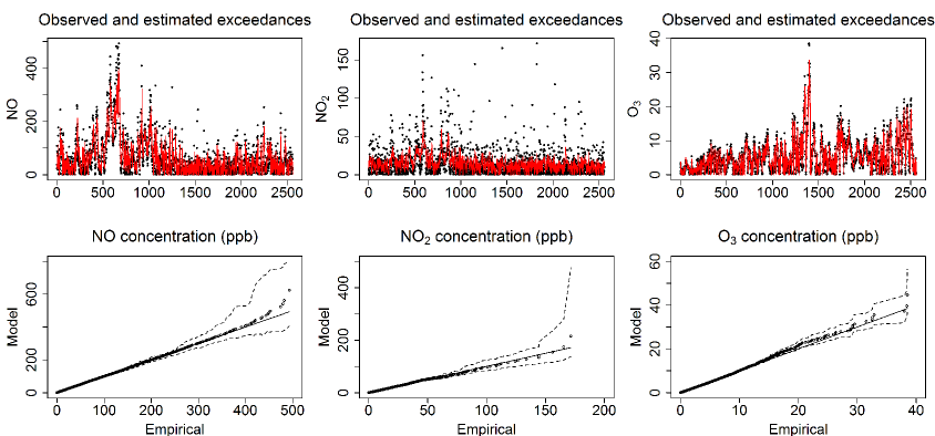
Figure 2: Top row: Observed threshold exceedances (dots) and their estimated conditional means (solid lines, red in the online version) for the three pollutants. Bottom row: QQ-plots of the overall model fit to the data, with straight lines indicating an exact agreement between the model and observations and dashed lines showing $95$%-credible intervals. The data used in these plots were reduced to keep only the exceedances without missing covariates; the number of usable data points was $2\mbox{$\>\!$}560$ (out of about $3\mbox{$\>\!$}500$), indexed in the top row plots in the order of appearance.

Analysing further the goodness-of-fit of the model, the plots of the observed threshold exceedances and their estimated posterior means are shown in the top row of Figure 2. (This figure is based on the data points for which all the covariates were recorded, resulting in a reduction of usable data from about $3\mbox{$\>\!$}500$ exceedances down to $2\mbox{$\>\!$}560$.) The expected value of the GPD (4) is given by $\mu^{u}_{\vphantom{t^{t}}\text{GPD}}=\sigma_{u}\mbox{$\>\!$}(1-\xi)^{-1}$ ($\xi<1$); in the nonstationary context, this is modified accordingly,

$$\mu^{u}_{\vphantom{t^{t}}\text{GPD}}(\boldsymbol{c})=\frac{\sigma_{u}(\boldsymbol{c})}{1-\xi(\boldsymbol{c})}.$$ (17)

The median $m^{u}_{\vphantom{t^{t}}\text{GPD}}=\sigma_{u}\mbox{$\>\!$}(2^{\xi}-1)/\xi$, as well as its nonstationary counterpart $m^{u}_{\vphantom{t^{t}}\text{GPD}}(\boldsymbol{c})$, has an advantage of being well defined for all $\xi\in\mathbb{R}$, but despite being robust against outliers the median is more “conservative” and may be a less spectacular benchmark for extreme value models because $m^{u}_{\vphantom{t^{t}}\text{GPD}}<\mu^{u}_{\vphantom{t^{t}}\text{GPD}}$ for $\xi>-1$.

The plots in Figure 2 show that the simulated data reproduce the observed threshold exceedances reasonably well, which again confirms the overall model fit. More specifically, for NO and especially for $\text{O}_{3}$ the match is quite good, but in the case of $\text{NO}_{2}$ many threshold exceedances are not well captured by the mean (nor by the median). The exact reason for that is not quite clear yet, but it is noteworthy that the $\text{NO}_{2}$ case stands out as the only one where the estimated shape parameter is positive, $\xi=0.074$ (see Section 4.3), suggesting that the posterior GPD of exceedances is rather heavy-tailed. In this case, the mean is less likely to be a faithful representative of large exceedances. Furthermore, it may be misleading to use the standard coefficient of determination $R^{2}$ as a measure of goodness-of-fit (Draper & Smith, 1998), because the coefficient $R^{2}$ is based on squared deviations from the mean, which could be extremely large due to heavy tails even if the model was in fact adequate. As an alternative, the conditional $95\%$-quantiles were calculated (not presented here), and it was concluded that the extreme concentrations were captured well by these higher quantiles. The overall conclusion is that the model has a good potential for an efficient determination of threshold exceedances from traffic and meteorological conditions.

Following Eastoe (2009), an alternative way to assess the model’s fit is to plot the observed order statistics of threshold exceedances against the order statistics obtained by simulation from the fitted model (cf. Section 3.6). Each of the simulated data sets has the same length as the observed data. The medians, along with $2.5\%$- and $97.5\%$-quantiles, were calculated for the order statistics from a simulated data set based on $1000$ replicas. The results presented in Figure 2 (bottom row) also confirm the overall good model fit.

4.3 Assessing the impact of the covariates

At the next step, the interest is in understanding the qualitative influence of the traffic and meteorological conditions on the magnitude and occurrence probability of extreme concentration values. This can be assessed by analysing the estimated parameters of the GPD as well as the conditional threshold exceedance probabilities. An optimal threshold probability that should be used to classify concentration values as extremes (i.e., lying above the threshold) can be determined by minimizing the total number of misclassified cases, that is, the total number of non-extremes classified as extremes and vice versa. The corresponding misclassification rates were found to be $7.13\%$ (NO), $8.26\%$ ($\text{NO}_{2}$) and $7.45\%$ ($\text{O}_{3}$). According to these results, the model is adequate to estimate the time occurrence of the threshold exceedances; therefore, it can be applied to describe the episodes of elevated air pollution concentrations.

In view of the equations (10), the average size of exceedances $X^{u}_{t}$ (see (17)) is a monotone transformation of linear combinations of the covariates. Hence, the coefficients of the regression model (10) characterize the size and direction of the impact of each variable on the threshold exceedances $X^{u}_{t}$. A similar interpretation is valid for the parameters describing the link between the covariates and the threshold exceedance rate $\rho_{u}(\boldsymbol{c})$.

Table 1 presents the results of estimation of the regression coefficients of various covariates for the averaged model, including the posterior medians, $95\%$-credible intervals and the posterior inclusion probabilities (note that the latter were consistently bigger than $0.05$ for almost all the covariates except for some higher-order Fourier terms of time variables).

Table 1: Estimated posterior medians and $95\%$-credible intervals of the regression coefficients (magnified by a factor of $10^{4}$) for the scale parameter $\sigma_{u}$ and the threshold exceedance rate $\rho_{u}$ in the model (10). The threshold level $u$ is chosen according to an empirical $90\%$-quantile. The posterior inclusion probabilities are presented in parentheses.

Covariates	Scale parameter $\sigma_{u}$			Threshold exceedance rate $\rho_{u}$
	NO	$\text{NO}_{2}$	$\text{O}_{3}$	NO	$\text{NO}_{2}$	$\text{O}_{3}$
TF (LDV)	$6.3$ $(0.25)$	$4.7$ $(0.47)$	$-2.8$ $(0.25)$	$37.4$ $(0.91)$	$38.2$ $(0.86)$	$-13.9$ $(0.88)$
	$[5.6,7.7]$	$[3.5,5.8]$	$[-3.2,-2.1]$	$[32.2,43.1]$	$[31.5,45.9]$	$[-18,-9.5]$
TF (HGV)	$10.5$ $(0.37)$	$3$ $(0.33)$	$-1.9$ $(0.39)$	$58.5$ $(0.84)$	$33.7$ $(0.79)$	$-20$ $(0.90)$
	$[8.4,12.0]$	$[2.0,5.7]$	$[-2.1,-1.2]$	$[34.2,69.7]$	$[22.5,42.0]$	$[-25.0,-15.6]$
TS (LDV)	$-5.0$ $(0.25)$	$-6.4$ $(0.78)$	$1.7$ $(0.13)$	$-6.7$ $(0.67)$	$-1.7$ $(0.89)$	$6.1$ $(0.55)$
	$[-5.2,-4.6]$	$[-7.6,-5.2]$	$[1.3,2.1]$	$[-9.5,-1.3]$	$[-2.4,-0.7]$	$[5.23,8.9]$
TS (HGV)	$-1.7$ $(0.27)$	$-2.5$ $(0.31)$	$0.79$ $(0.37)$	$-7.2$ $(0.79)$	$-1.0$ $(0.12)$	$4.1$ $(0.69)$
	$[-1.9,-1.5]$	$[-3.8,-1.2]$	$[0.4,1.2]$	$[-10.5,-2.8]$	$[-1.6,-0.5]$	$[3.3,4.9]$
WS	$-3.1$ $(0.83)$	$4.4$ $(0.63)$	$1.9$ $(0.80)$	$-4.2$ $(0.90)$	$-2.0$ $(0.10)$	$9.3$ $(0.90)$
	$[-3.5,-2.6]$	$[3.9,6.1]$	$[1.6,2.3]$	$[-5.0,-3.7]$	$[-2.9,-1.4]$	$[4.8,15.6]$
RH	$2.3$ $(0.70)$	$1.6$ $(0.30)$	$-1.2$ $(0.30)$	$0.15$ $(0.90)$	$3.0$ $(0.86)$	$-1.5$ $(0.44)$
	$[2.0,2.6]$	$[1.0,2.8]$	$[-1.5,-1.0]$	$[0.1,0.2]$	$[2.1,4.2]$	$[-1.9,-1.0]$
T	$-1.6$ $(0.27)$	$-1.7$ $(0.53)$	$2.6$ $(0.28)$	$-3.3$ $(0.78)$	$-2.58$ $(0.78)$	$1.3$ $(0.15)$
	$[-1.8,-1.6]$	$[-2.3,-0.9]$	$[1.9,3.2]$	$[-3.6,-2.8]$	$[-3.4,-1.9]$	$[0.9,1.96]$
SR	$-3.5$ $(0.62)$	$-1.3$ $(0.38)$	$4.0$ $(0.51)$	$-0.9$ $(0.93)$	$-2.0$ $(0.93)$	$3.9$ $(0.81)$
	$[-4.2,-3.5]$	$[-2.6,-0.7]$	$[1.8,6.7]$	$[-1.4,-0.5]$	$[-2.6,-1.5]$	$[2.9,4.5]$

Note that with a higher traffic flow for both LDV and HGV categories, the size and probability of threshold exceedances increase for $\text{NO}_{x}$ and decrease for $\text{O}_{3}$. The traffic speed has an opposite effect on the size and exceedance probability for each pollutant, which can be explained by the negative correlation between the traffic speed and traffic flow. In practice, the speed is not entirely negatively correlated with the flow; a positive correlation may arise when the traffic conditions change from “busy” to “congested” (Bell et al., 2006). According to the estimated coefficients of the traffic regimes (factors), the size and probability of threshold exceedances increase as the traffic changes from “quiet” towards “congested”, in agreement with Bell et al. (2006).

From the estimated weekly Fourier components of the time variables (not shown in the table), there are decreased levels of $\text{NO}_{x}$ and an increased level of ozone at weekends, as could be expected due to decreased traffic volume and emission of possible point sources (e.g., factories). On the other hand, $\text{NO}_{x}$ levels decrease with temperature and solar radiation, which is a manifestation of the photochemical nature of the chemical reaction between these pollutants. The estimated coefficients of daily Fourier component variables, and their second-order terms, suggest that there is a significant difference between daylight and night-time levels, as well as between peak and off-peak hours, with higher vs. lower average concentrations, respectively. Increased $\text{NO}_{x}$ (decreased $\text{O}_{3}$) concentrations can be observed during the winter months, contrasted with decreased $\text{NO}_{x}$ (increased $\text{O}_{3}$) concentrations during the summer months. Furthermore, stronger winds correspond to decreased levels of NO and increased levels of $\text{NO}_{2}$ and $\text{O}_{3}$, which is likely to be due to the transport mechanisms and mixing of the particles at this particular site.

Model II preserving the threshold stability was fitted to the data using the similar MCMC procedure as for Model I (see Section 3.3). It is assumed that the parameters $\alpha(\boldsymbol{c})$ and $\gamma(\boldsymbol{c})$ are linear functions of the same covariates as in Model I, while $\beta(\boldsymbol{c})\equiv\beta$ is constant (see equations (12)). The sign of the shape parameter $\xi$ for different pollutants (determined by the sign of $\beta$) is the same as in Model I, that is, the corresponding GPD is bounded for NO and $\text{O}_{3}$, and is heavy-tailed for $\text{NO}_{2}$. The results obtained for the estimated shape parameter $\xi$ are shown as part of Table 2, and are very similar to those in Model I. Note however that the estimated medians for $\xi$ are slightly lower for Model II as compared to Model I, so that the former is more conservative in predicting high exceedances. This trend is also confirmed by computing the estimated return levels (see Table 3).

Table 2: Estimated posterior medians for the shape parameter $\xi$ and the corresponding $95\%$-credible intervals (CI) in Models I and II.

Pollutant	Model I		Model II
	$\xi$	$95\%$-CI	$\xi$	$95\%$-CI
NO	$-0.101$	$[-0.114,-0.081]$	$-0.148$	$[-0.156,-0.127]$
$\text{NO}_{2}$	$\hphantom{-}0.074$	$[0.038,0.103]$	$\hphantom{-}0.061$	$[0.043,0.091]$
$\text{O}_{3}$	$-0.279$	$[-0.296,-0.259]$	$-0.292$	$[-0.301,-0.274]$

One can also plot the estimated medians on top of the observed exceedances, as was done for Model I in Figure 2. The results (not shown here) are very similar, but again suggest that the estimates under Model II tend to be slightly lower. The results of estimation of the shape parameter $\xi$ in Models I and II are presented in Table 2. In particular, it appears that the posterior distribution of $\xi$ is likely to be bounded above for NO and $\text{O}_{3}$ (Weibull type GPD), while being heavy-tailed for $\text{NO}_{2}$ (Fréchet type GPD).

4.4 Cross-validation

The possibility of overfitting as well as the predictive strength of the model were investigated by using cross-validation. Each month was divided into two parts — the first $75\%$ of the data were used for the model calibration and the remaining $25\%$ for the model validation. Inference about the predictive strength of the model was drawn by using the same diagnostics presented in the previous sections. The results are very similar to those presented in Figure 2, and therefore are not shown here.

In the prediction of the conditional probability of threshold exceedance, the corresponding misclassification rates were $10.23\%$ (NO), $11.01\%$ ($\text{NO}_{2}$), and $10.79\%$ ($\text{O}_{3}$). These results show that the model predicts extreme concentrations and their occurrence probability quite successfully, and the risk of overfitting is low.

4.5 Bayesian model comparison

Although a bare-eye inspection of the graphical results does not reveal much difference between the models, they can be compared quantitatively using the so-called Bayes factor (Kass & Raftery, 1995), defined as the likelihood ratio for Model II ($\text{M}_{2}$) against Model I ($\text{M}_{1}$),

$$B_{21}:=\frac{L(\text{M}_{2}\mbox{$\>\!$}|\mbox{$\>\!$}\boldsymbol{X})}{L(\text{M}_{1}\mbox{$\>\!$}|\mbox{$\>\!$}\boldsymbol{X})},$$

where $\boldsymbol{X}$ denotes the threshold exceedance data and $L(\text{M}_{i}\mbox{$\>\!$}|\mbox{$\>\!$}\boldsymbol{X})=f(\boldsymbol{X}\mbox{$\>\!$}|\mbox{$\>\!$}\text{M}_{i})$ is the likelihood (joint density) under the model $\text{M}_{i}$. The reference value of the Bayes factor is $B_{21}=1$, corresponding to no preference for either of the models, while values greater or smaller than $1$ show evidence in favour of the model $\text{M}_{2}$ or the alternative model $\text{M}_{1}$, respectively. It is more convenient to work with the quantity $\beta_{21}=2\ln B_{21}$, for which an indicative scale was given by Kass and Raftery (1995); for example, the values of $\beta_{21}$ in the range 2–5 or 5–10 are interpreted respectively as positive or strong evidence in favour of the model $\text{M}_{2}$ against the competing model $\text{M}_{1}$.

For our data, the calculated Bayes log-factor $\beta_{21}$ is $6.28$ (NO),  $5.57$ ($\text{NO}_{2}$), and $7.49$ ($\text{O}_{3}$); thus, according to the above classification the threshold-stable model $\text{M}_{2}$ strongly outperforms the Davison–Smith type model $\text{M}_{1}$.

This result was also validated and confirmed using an alternative model selection procedure called the deviance information criterion (DIC) (results not shown here). This criterion is widely used in the Bayesian setting to handle complex models with abundance of possible parameters (see Claeskens & Hjort, 2008).

4.6 The models’ performance under decreased traffic flow

To illustrate the flexibility of the models, possible future scenarios corresponding to a $25\%$-decrease in the traffic flow were generated and the drop in the marginal return level was assessed. Note that the simulation method described in Section 3.6 cannot be used without modification; indeed, resampling the lagged concentration values directly from the empirical distribution of the values below the threshold (i.e., $X_{t}\leq u$) from the same daylight (7am–8pm) or night-time (8pm–7am) of the corresponding day would lead to a bias because the reduction in the traffic flow would be ignored. To overcome this problem, the past concentration values were resampled from the subset of values $(X_{t})$ satisfying $X_{t}\leq u$ and belonging to the time period of the corresponding daylight or night-time when the traffic flow is between $70\%$ and $80\%$ of the total traffic flow observed at time $t$. If this interval was empty then the observed lagged concentration values corresponding to time $t$ were kept.

Table 3: Estimated 5- and 10-year return levels for the observed and $25\%$-decreased traffic flow conditions in Models I and II. Point estimates and posterior $95\%$-credible intervals were obtained by simulation.

	Observed flow		Decreased flow
	5-year	10-year	5-year	10-year
Model I
NO	$988.4$	$1264.1$	$882.0$	$1055.5$
	$[591.2,1325.9]$	$[780.6,1625.4]$	$[536.8,1151.5]$	$[669.3,1543.9]$
$\ \,\text{NO}_{2}$	$362.3$	$426.3$	$313.1$	$376.9$
	$[251.1,530.5]$	$[291.8,602.5]$	$[216.0,466.6]$	$[253.4,529.6]$
$\text{O}_{3}$	$94.5$	$99.6$	$96.7$	$102.4$
	$[86.9,107.9]$	$[89.6,110.5]$	$[89.1,111.8]$	$[93.7,115.0]$
Model II
NO	$959.2$	$1214.6$	$859.7$	$1024.7$
	$[551.9,1292.5]$	$[763.9,1583.9]$	$[519.8,1139.4]$	$[652.6,1517.7]$
$\ \,\text{NO}_{2}$	$336.6$	$380.9$	$288.8$	$331.1$
	$[237.8,499.3]$	$[277.7,566.4]$	$[238.3,334.3]$	$[246.5,467.6]$
$\text{O}_{3}$	$91.3$	$97.1$	$97.0$	$104.1$
	$[83.8,102.9]$	$[85.8,107.4]$	$[91.5,114.9]$	$[94.1,117.1]$

Table 3 illustrates the $5$- and $10$-year marginal return levels estimated with the original covariates, as well as with those corresponding to a reduced traffic flow. Note that there is a noticeable drop in return levels for each scenario under Model II as compared to Model I. To assess if these estimates are realistic, additional concentration values were analysed for cross-validation. Altogether, two years worth of concentration data were available from the monitoring site covering the period from November 1, 2007 till November 1, 2009; unfortunately, only the period from January 1, 2008 to January 1, 2009 could be used for modelling purposes due to missing traffic or meteorological observations outside this period.

The observed maxima for the $2$-year data were $811.1$ (NO), $245.2$ ($\text{NO}_{2}$), and $80.5$ ($\text{O}_{3}$), whereas the observed $1$-year maxima were $574.8$, $220.3$, and $80.5$, respectively. Overall, these results provide additional evidence that the estimated 5-year return levels can be considered as realistic.

5 Discussion and conclusions

Modelling and predicting air pollution episodes is commonly believed to be a formidable task, especially on a short time scale. The inherent difficulties are due to the complexity and dynamic nature of traffic conditions and meteorological characteristics interwoven with photochemical reactions in the atmosphere. In this paper, the classical model of Davison and Smith (1990) was adapted so as to incorporate nonstationary traffic and weather covariates into the POT statistical analysis of pollution extremes (Model I). Furthermore, a modified version of the Davison–Smith model aiming to ensure the threshold stability was derived (Model II) and its performance was compared to that of Model I. The estimation and a model selection procedure were carried out using a suitable MCMC algorithm. Both models demonstrated a good fit to the data; however, using a Bayesian hypothesis testing it was concluded that Model II significantly outperformed Model I.

The models discussed in this paper yield encouraging results and have a promising potential for an accurate and reliable estimation of extreme concentrations. Owing to their regression-based structure, they are easy to implement in practice. Most importantly, the models can be used to draw predictive inference about extreme values beyond the observed ranges and, consequently, to design, validate and evaluate future air pollution scenarios, for example, resulting from changing patterns in the traffic flow and/or meteorological conditions. Thus, our models can provide the air quality decision makers with an effective tool to manage air pollution problems.

As compared to a similar model developed by Eastoe and Tawn (2009) in the context of surface level ozone ($\text{O}_{3}$) concentrations, a required improvement achieved in the present work is the inclusion of the traffic-related covariates, which turn out to be significant under both models. Despite confining ourselves to univariate models for each chemical, it should be noted that the need to account for multiple pollutants is somewhat addressed in our paper owing to the use of a regression framework in the MCMC simulation; hence, due to lagged past values of the pollutant in question (e.g., NO), the impact of other (correlated) pollutants (such as $\text{NO}_{2}$ and $\text{O}_{3}$) is implicitly taken into account. Furthermore, these models may serve as a stepping stone for a multivariate version of the POT modelling in the air pollution context (cf. Roth et al., 2014), which will be developed in our forthcoming work. It would also be important to add a spatial (e.g., regional) dimension to the models, in particular due to the apparent significance of proximity to point sources such as factories or road junctions. To this end, data available from the UK’s largest database known as the Automatic Urban and Rural Network (AURN, 2016) will be instrumental (cf. Gyarmati-Szabó et al., 2011).

The issue of choosing a “correct” threshold in the nonstationary POT modelling has attracted a lot of attention due to its paramount importance for the extreme value inference (Northrop & Jonathan, 2011; Northrop & Coleman, 2014). Following the classic approach by Davison and Smith (1990), further developed in the environmental context, for example, by Eastoe and Tawn (2009), we have opted to work in this paper with a constant threshold (determined by a certain empirical quantile, e.g., $90\%$) and to model nonstationarity of the data through dependence on time-varying covariates. The alternative popular approach is to choose a time-dependent, data-driven threshold (using some graphical diagnostics) but to keep the parameters of the GPD constant (Northrop et al., 2016; Northrop et al., 2017). The latter idea is appealing, because the exceedance rate of a fixed threshold may deteriorate due to nonstationarity; thus, it is reasonable to monitor the estimation performance and adjust the threshold if and when necessary. Flexibility with the threshold is also attractive in view of the possible future changes (e.g., in the environmental standards, driving patterns or climate). From this point of view, the threshold-stable Model II proposed in this work is conceptually rather promising. The fact that we do not seem to use its full potential is somewhat deceiving: as argued in the paper (see Section 3.2), the model fitting should be done only once for a chosen threshold — should it change, the GPD parameters are easily recalculated, whereas the exceedance rate can be computed using formula (9). Thus, in a sense, Model II may serve to bridge the gap between the two alternative approaches to the threshold selection.

Finally, let us point out that the successful extreme value modelling also crucially relies on the quality of the data collected. Air pollution concentrations are known to be significantly location-dependent as well as highly variable temporally, with noticeable deviations from stationarity. Pervasive mobile environmental sensors, developed for example in the MESSAGE project (MESSAGE, 2009), could provide a cost-effective, accurate monitoring system. Air quality data from such a grid, combined with the urban big data (e.g., UBDC, 2017), would be instrumental for both feeding in and validating the extreme value models developed in this study and, as a consequence, should prove valuable for evidence-based air quality decision-making.

References

- AURN. (2016). Automatic Urban and Rural Network (AURN). Department for Environment, Food & Rural Affairs (DEFRA, UK). Available online at uk-air.defra.gov.uk/networks/network-info?view=aurn.
- Beirlant, J., Goegebeur, Y., Teugels, J., & Segers, J. (2004). Statistics of extremes: theory and applications. Chichester: Wiley. doi:10.1002/0470012382
- Bell, M., Chen, H., Hackman, M., McCabe, K., & Price, S. (2006). Using ITS to reduce environmental impacts. In 13th World Congress on Intelligent Transport Systems and Services (8–12 October 2006, London, UK), Paper 1271. World Road Association — PIARC. Retrieved from https://www.academia.edu/29090250/Using_ITS_to_Reduce_Environmental_Impacts.
- Carslaw, D. C., Beevers, S. D., & Tate, J. E. (2007). Modelling and assessing trends in traffic-related emissions using a generalised additive modelling approach. Atmospheric Environment, 41, 5289–5299. doi:10.1016/j.atmosenv.2007.02.032
- Claeskens, G., & Hjort, N. L. (2008). Model selection and model averaging. Cambridge: Cambridge University Press. doi:10.1017/CBO9780511790485
- Clapp, L. J., & Jenkin, M. E. (2001). Analysis of the relationship between ambient levels of , and NO as a function of in the UK. Atmospheric Environment, 35, 6391–6405. doi:10.1016/S1352-2310(01)00378-8
- Coles, S. (2001). An introduction to statistical modeling of extreme values. London: Springer. doi:10.1007/978-1-4471-3675-0
- Davison, A. C., & Smith, R. L. (1990). Models for exceedances over high thresholds. Journal of the Royal Statistical Society, Series B (Methodological), 52, 393–442. www.jstor.org/stable/2345667
- Draper, N. R., & Smith, H. (1998). Applied regression analysis (3rd ed.). New York: Wiley. doi:10.1002/9781118625590
- Eastoe, E. F. (2009). A hierarchical model for non-stationary multivariate extremes: a case study of surface-level ozone and data in the UK. Environmetrics, 20, 428–444. doi:10.1002/env.938
- Eastoe, E. F., & Tawn, J. A. (2009). Modelling non-stationary extremes with application to surface level ozone. Journal of the Royal Statistical Society, Series C (Applied Statistics), 58, 25–45. doi:10.1111/j.1467-9876.2008.00638.x
- Embrechts, P., Klüppelberg, C., & Mikosch, T. (1997). Modelling extremal events for insurance and finance. New York: Springer. doi:10.1007/978-3-642-33483-2
- Gilks, W. R., Richardson, S., & Spiegelhalter, D. J. (eds.) (1996). Markov Chain Monte Carlo in practice. London: Chapman and Hall/CRC Press.
- Gyarmati-Szabó, J., Bogachev, L. V., & Chen, H. (2011). Modelling threshold exceedances of air pollution concentrations via non-homogeneous Poisson process with multiple change-points. Atmospheric Environment, 45, 5493–5503. doi:10.1016/j.atmosenv.2011.06.049
- Horowitz, J., & Barakat, S. (1979). Statistical analysis of the maximum concentration of an air pollutant: effects of autocorrelation and non-stationarity. Atmospheric Environment, 13, 811–818. doi:10.1016/0004-6981(79)90272-5
- Kass, R. E., & Raftery, A. E. (1995). Bayes factors. Journal of the American Statistical Association, 90(430), 773–795. doi:10.1080/01621459.1995.10476572
- Küchenhoff, H., & Thamerus, M. (1996). Extreme value analysis of Munich air pollution data. Environmental and Ecological Statistics, 3, 127–141. doi:10.1007/BF02427858
- Kuo, L., & Mallick, B. (1998). Variable selection for regression models. Sankhyā: The Indian Journal of Statistics, Series B, 60, 65–81. https://www.jstor.org/stable/25053023?seq=1#page_scan_tab_contents
- Madigan, D., & Raftery, A. E. (1994). Model selection and accounting for model uncertainty in graphical models using Occam’s window. Journal of the American Statistical Association, 89(428), 1535–1546. doi:10.1080/01621459.1994.10476894
- MESSAGE. (2009). Mobile Environmental Sensing System Across Grid Environments (MESSAGE). Research Project, grants SRT 7/5/7 (DfT) and (EPSRC), 2006–2009. Retreived from webarchive.nationalarchives.gov.uk/20140603191607/http://www.dft.gov.uk/rmd/project.asp?intProjectID=12457
- Northrop, P. J., Attalides, N., & Jonathan, P. (2017). Cross-validatory extreme value threshold selection and uncertainty with application to ocean storm severity. Journal of the Royal Statistical Society: Series C (Applied Statistics), 66, 93–120. doi:10.1111/rssc.12159
- Northrop, P. J., & Coleman, C. L. (2014). Improved threshold diagnostic plots for extreme value analyses. Extremes, 17, 289–303. doi:10.1214/09-BA403
- Northrop, P. J., & Jonathan, P. (2011). Threshold modelling of spatially dependent non-stationary extremes with application to hurricane-induced wave heights. Environmetrics, 22, 799–809. doi:10.1002/env.1106
- Northrop, P. J., Jonathan, P., & Randell, D. (2016). Threshold modeling of nonstationary extremes. In Extreme value modeling and risk analysis: methods and applications (Dey, D. K., & Yan, J., eds.), Boca Raton, FL: Chapman and Hall/CRC Press, pp. 87–108. doi:10.1007/s10687-014-0183-z
- O’Hara, R. B., & Sillanpää, M. J. (2009). A review of Bayesian variable selection methods: what, how and which. Bayesian Analysis, 4, 85–118. doi:10.1214/09-BA403
- Pickands, J. (1975). Statistical inference using extreme order statistics. The Annals of Statistics, 3, 119–131. doi:10.1214/aos/1176343003
- Roth, M., Buishand, T. A., Jongbloed, G., Klein Tank, A. M. G., & van Zanten, J. H. (2014). Projections of precipitation extremes based on a regional, non-stationary peaks-over-threshold approach: a case study for the Netherlands and north-western Germany. Weather and Climate Extremes, 4, 1–10. doi:10.1016/j.wace.2014.01.001
- Smith, R. L. (1989). Extreme value analysis of environmental time series: an application to trend detection in ground-level ozone. Statistical Science, 4, 367–377. doi:10.1214/ss/1177012400
- Thompson, M. L., Reynolds, J., Cox, L. H., Guttorp, P., & Sampson, P. D. (2001). A review of statistical methods for the meteorological adjustment of tropospheric ozone. Atmospheric Environment, 35, 617–630. doi:10.1016/S1352-2310(00)00261-2
- UBDC. (2017). Urban Big Data Centre (UBDC), University of Glasgow, UK. Funded by the ESRC (the Economic and Social Research Council, UK). Available online at http://ubdc.ac.uk/.
- WHO. (2000). Air quality guidelines for Europe (2nd ed.). World Health Organization (WHO) Regional Publications, European Series, No. 91. Copenhagen: Regional Office for Europe. Available online at www.euro.who.int/__data/assets/pdf_file/0005/74732/E71922.pdf.
- Zito, P., Chen, H., & Bell, M. C. (2008). Predicting real-time roadside CO and concentrations using neural networks. IEEE Transactions on Intelligent Transportation Systems, 9, 514–522. doi:10.1109/TITS.2008.928259