Understanding experimentally-observed fluctuations

Abstract

We discuss two topics on the experimental measurements of fluctuation observables in relativistic heavy-ion collisions. First, we discuss the effects of the thermal blurring, i.e. the blurring effect arising from the experimental measurement of fluctuations in momentum space as a proxy of the thermal fluctuations defined in coordinate space, on higher order cumulants. Second, we discuss the effect of imperfect efficiency of detectors on the measurement of higher order cumulants. We derive effective formulas which can carry out the correction of this effect for higher order cumulants based on the binomial model.

1 Introduction

Fluctuations of conserved charges are important observables in relativistic heavy-ion collisions because they are believed to be sensitive to early thermodynamics of the hot medium created by the collisions [1]. Active theoretical and experimental studies on the fluctuation observables as well as numerical simulations on the lattice and their comparison have been carried out. In particular, non-Gaussianity of fluctuations characterized by higher-order cumulants acquires much attention recently. For example, the sign of higher-order cumulants is believed to be sensitive to the location of a medium in the QCD phase diagram [2, 3].

In theoretical studies and lattice simulations on fluctuation observables, they are usually studied based on statistical mechanics. The fluctuations discussed in this formalism are called thermal fluctuations. On the other hand, the experimental analyses measure the event-by-event fluctuations of particle number observed by detectors. Although these fluctuations are sometimes compared directly in the literature, the experimentally-observed fluctuations are not the same as the thermal fluctuations in various aspects. In this talk, we focus on two such differences [4, 5], and clarify the reason why they are different and in which case they can be compared with each other. We also discuss practical ways to compare these different fluctuations.

2 Thermal blurring

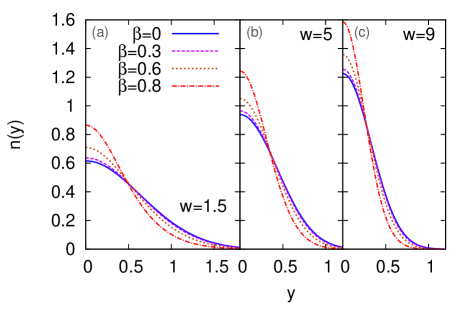
Figure 1: Particle number distribution per unit rapidity $n(y)$ for several values of $w=m/T$ and the transverse velocity $\beta$ [4].

We first focus on the difference in phase spaces in which thermal fluctuations and the fluctuation observed in experiments are defined [4]. First, thermal fluctuations calculated in statistical mechanics are those in a spatial volume with momentum space integrated out. On the other hand, the experimental detectors can only measure the momentum of particles entering there. Therefore, the event-by-event fluctuations measured in experiments are inevitably those in a momentum phase space. Therefore, the phase spaces defining fluctuations are completely different between theoretical and experimental settings.

Nevertheless, for sufficiently high energy collisions the latter can be regarded as a proxy of the former as recognized in earlier studies [6, 7]. This approximate correspondence can be obtained by assuming the Bjorken space-time evolution. In this space-time picture, the system has boost invariance. Accordingly, (momentum-space) rapidity and coordinate-space rapidity,

$$y=\frac{1}{2}\ln\frac{E-p_{z}}{E+p_{z}},\quad Y=\frac{1}{2}\ln\frac{t-z}{t+z},$$ (1)

of a fluid element are equivalent in this picture, where $z$ represents the longitudinal coordinate. If all particles were stopping in each fluid element, therefore, the experimental measurement in a rapidity window $\Delta y$ can be regarded as the one in the coordinate-space rapidity window with $\Delta Y=\Delta y$.

However, particles have thermal motion, and thus they have nonzero velocity in the rest frame of a fluid element. The correspondence between $y$ and $Y$ thus is only an approximate one for individual particles. Due to this difference, the experimental measurement of a particle number in $\Delta y$ receives a blurring effect when it is interpreted as the coordinate-space one in $\Delta Y$. We call this effect as thermal blurring. In Fig. 1, we show the thermal distribution of a free particle with mass $m$ in rapidity space in a medium with temperature $T$ and radial velocity $\beta$. The result is plotted for various values of $w=m/T$. The blastwave model for the central collisions at LHC and top-RHIC energies suggests $T\simeq 100$ MeV and $\beta=0.6-0.7$ at kinetic freezeout; thus pions have $w\simeq 1.5$ while nucleons have $w\simeq 9$ at kinetic freezeout. From Fig. 1, one finds that for pions the thermal width in $y$ space is as large as $1.0$, which is comparable with the maximum coverage of the STAR detector $\Delta y=1.0$. This result indicates that the measurement of net-electric charge fluctuation at STAR is strongly affected by the thermal blurring effect. When the event-by-event fluctuation at $\Delta y=1.0$ is compared with the thermal one, therefore, the thermal blurring effect has to be considered seriously.

In Ref. [4], it is discussed that the thermal blurring effect gives rise to a characteristic dependence of higher-order cumulants as a function of $\Delta y$. This result suggests that the experimental result of the cumulants as a function of $\Delta y$ can be used to understand and remove the thermal blurring effect. It is also discussed that the thermal blurring can be regarded as a part of diffusion before kinetic freezeout [8]. It is an interesting subject to investigate the $\Delta y$ dependences of higher-order cumulants experimentally, and extract the values of cumulants before the blurring and diffusion effects. See Ref. [8] for more detailed discussion.

3 Efficiency correction

Next, we consider the effect of the imperfect efficiency of detectors on fluctuation observables [5]. All detector can measure particles entering there only with a probability less than unity, which is called the efficiency. Because of the finite efficiency, the event-by-event distribution of a particle number observed experimentally is different from the original one without the efficiency loss. The cumulants characterizing the distribution function, therefore, are also modified by the efficiency loss. This difference has to be corrected in experimental analyses to remove the artificial effect due to the efficiency loss.

It is known that this procedure for efficiency correction can be carried out when the efficiencies for individual particle are independent [9]. In this case, the event-by-event probability distribution functions of observed and original particle numbers are related with each other in a simple form with binomial distribution functions [9]. Using this relation, the cumulants of original particle number without efficiency loss can be represented by those of observed particle numbers with efficiency loss. These relations are first obtained for net-particle number with two different efficiencies for particle and anti-particle [9]. The relation is then extended to the case that the particle number is given by a sum of the numbers of different species of particles which are observed with different efficiencies [10, 11].

The procedure of the efficiency correction presented in Refs. [10, 11] is given in terms of factorial moments. In this method, however, the number of factorial moments grows as the number of different particle species $M$ increases. Accordingly, the numerical cost required for the efficiency correction becomes large rapidly with increasing $M$; for $n$-th order cumulant, the cost increases $\sim M^{n}$. In order to carry out the efficiency correction with a reasonable computational time, therefore, the number of $M$ is limited to a small number.

In Ref. [5], different formulas which lead to the same result as those in Refs. [10, 11] are obtained. In this formula, the efficiency correction of a charge which is given by

$$Q=\sum_{i=1}^{M}a_{i}N_{i},$$ (2)

is considered, where $N_{i}$ is a particle number with a species of particle labeled by $i$, and $a_{i}$ is a numerical number. Because of the efficiency loss, the number $n_{i}$ observed by the detector can be different from, and typically smaller than, $N_{i}$. The cumulants of $Q$ up to fourth order are given by

$$\langle Q\rangle_{\rm c} = \mathopen{\hbox{${\langle}$}\mkern 2.0mu\kern-3.49998pt\leavevmode\hbox{${\langle}$}}q_{(1)}\mathclose{\hbox{${\rangle}$}\mkern 2.0mu\kern-3.49998pt\leavevmode\hbox{${\rangle}$}}_{\rm c},$$ (3)

$$\langle Q^{2}\rangle_{\rm c} = \mathopen{\hbox{${\langle}$}\mkern 2.0mu\kern-3.49998pt\leavevmode\hbox{${\langle}$}}q_{(1)}^{2}\mathclose{\hbox{${\rangle}$}\mkern 2.0mu\kern-3.49998pt\leavevmode\hbox{${\rangle}$}}_{\rm c}-\mathopen{\hbox{${\langle}$}\mkern 2.0mu\kern-3.49998pt\leavevmode\hbox{${\langle}$}}q_{(2)}\mathclose{\hbox{${\rangle}$}\mkern 2.0mu\kern-3.49998pt\leavevmode\hbox{${\rangle}$}}_{\rm c},$$ (4)

$$\langle Q^{3}\rangle_{\rm c} = \mathopen{\hbox{${\langle}$}\mkern 2.0mu\kern-3.49998pt\leavevmode\hbox{${\langle}$}}q_{(1)}^{3}\mathclose{\hbox{${\rangle}$}\mkern 2.0mu\kern-3.49998pt\leavevmode\hbox{${\rangle}$}}_{\rm c}-3\mathopen{\hbox{${\langle}$}\mkern 2.0mu\kern-3.49998pt\leavevmode\hbox{${\langle}$}}q_{(2)}q_{(1)}\mathclose{\hbox{${\rangle}$}\mkern 2.0mu\kern-3.49998pt\leavevmode\hbox{${\rangle}$}}_{\rm c}+\mathopen{\hbox{${\langle}$}\mkern 2.0mu\kern-3.49998pt\leavevmode\hbox{${\langle}$}}3q_{(2,1|2)}-q_{(3)}\mathclose{\hbox{${\rangle}$}\mkern 2.0mu\kern-3.49998pt\leavevmode\hbox{${\rangle}$}}_{\rm c},$$ (5)

$$\langle Q^{4}\rangle_{\rm c} = \mathopen{\hbox{${\langle}$}\mkern 2.0mu\kern-3.49998pt\leavevmode\hbox{${\langle}$}}q_{(1)}^{4}\mathclose{\hbox{${\rangle}$}\mkern 2.0mu\kern-3.49998pt\leavevmode\hbox{${\rangle}$}}_{\rm c}-6\mathopen{\hbox{${\langle}$}\mkern 2.0mu\kern-3.49998pt\leavevmode\hbox{${\langle}$}}q_{(2)}q_{(1)}^{2}\mathclose{\hbox{${\rangle}$}\mkern 2.0mu\kern-3.49998pt\leavevmode\hbox{${\rangle}$}}_{\rm c}+12\mathopen{\hbox{${\langle}$}\mkern 2.0mu\kern-3.49998pt\leavevmode\hbox{${\langle}$}}q_{(2,1|2)}q_{(1)}\mathclose{\hbox{${\rangle}$}\mkern 2.0mu\kern-3.49998pt\leavevmode\hbox{${\rangle}$}}_{\rm c}+3\mathopen{\hbox{${\langle}$}\mkern 2.0mu\kern-3.49998pt\leavevmode\hbox{${\langle}$}}q_{(2)}^{2}\mathclose{\hbox{${\rangle}$}\mkern 2.0mu\kern-3.49998pt\leavevmode\hbox{${\rangle}$}}_{\rm c}$$ (6)

$$-4\mathopen{\hbox{${\langle}$}\mkern 2.0mu\kern-3.49998pt\leavevmode\hbox{${\langle}$}}q_{(3)}q_{(1)}\mathclose{\hbox{${\rangle}$}\mkern 2.0mu\kern-3.49998pt\leavevmode\hbox{${\rangle}$}}_{\rm c}+\mathopen{\hbox{${\langle}$}\mkern 2.0mu\kern-3.49998pt\leavevmode\hbox{${\langle}$}}-15q_{(2,2|2)}+6q_{(2,1,1|3)}+4q_{(3,1|2)}-q_{(4)}\mathclose{\hbox{${\rangle}$}\mkern 2.0mu\kern-3.49998pt\leavevmode\hbox{${\rangle}$}}_{\rm c},$$

where the cumulants $\langle\cdot\rangle_{\rm c}$ and $\mathopen{\hbox{${\langle}$}\mkern 2.0mu\kern-3.49998pt\leavevmode\hbox{${\langle}$}}\cdot\mathclose{\hbox{${\rangle}$}\mkern 2.0mu\kern-3.49998pt\leavevmode\hbox{${\rangle}$}}_{\rm c}$ are taken for original distribution function for $N_{i}$ and observed one for $n_{i}$, respectively. $q_{(\cdots)}$ are linear combinations of $n_{i}$ defined by

$$q_{(s)}=\sum_{i=1}^{M}c_{(s)}^{(i)}n_{i},\qquad q_{(s_{1},\cdots,s_{j}|t_{1},\cdots,t_{k})}=\sum_{i=1}^{M}c_{(s_{1},\cdots,s_{j}|t_{1},\cdots,t_{k})}^{(i)}n_{i}.$$ (7)

The coefficients $c_{(\cdots)}^{(i)}$ are numerical numbers which depend on $a_{i}$ and $\epsilon_{i}$ defined by

$$c_{(s)}^{(i)}=\tilde{a}_{i}^{s}\tilde{\xi}_{s}^{(i)},\qquad c_{(s_{1},\cdots,s_{j}|t_{1},\cdots,t_{k})}^{(i)}=\tilde{a}_{i}^{s_{1}+\cdots+s_{j}}\tilde{\xi}_{s_{1}}^{(i)}\cdots\tilde{\xi}_{s_{j}}^{(i)}\tilde{\xi}_{t_{1}}^{(i)}\cdots\tilde{\xi}_{t_{k}}^{(i)},$$ (8)

with $\tilde{a}_{i}=a_{i}/\epsilon_{i}$, $\tilde{\xi}_{m}^{(i)}=\xi_{m}^{(i)}/\epsilon_{i}$, and $\xi_{m}^{(i)}=\xi_{m}(\epsilon_{i})$ being coefficients of the binomial cumulants with probability $\epsilon_{i}$.

Equations (3) – (6) represent the cumulants of the original particle number $Q$ by the mixed cumulants of observed particle numbers. Since the right-hand sides in these equations are experimental observables, these equations enable the efficiency correction. The formulas Eqs. (3) – (6) consist of a fixed number of mixed cumulants. Because of this property, the numerical cost for the efficiency correction is proportional to $M$ for all orders of cumulants. This is contrasted to the numerical cost of the method in Refs. [10, 11] which is proportional to $M^{n}$. The new formula can drastically reduce the numerical cost especially when $M$ and $n$ are large. Because of this advantage, Eqs. (3) – (6) will enable us to carry out the efficiency corrections with momentum dependent efficiency. It is an important subject to perform such efficiency corrections in experimental analyses.

References

- [1] M. Asakawa and M. Kitazawa, Prog. Part. Nucl. Phys. 90 (2016) 299.
- [2] M. Asakawa, S. Ejiri, and M. Kitazawa, Phys. Rev. Lett. 103 (2009) 262301.
- [3] M. A. Stephanov, Phys. Rev. Lett. 107 (2011) 052301.
- [4] Y. Ohnishi, M. Kitazawa and M. Asakawa, Phys. Rev. C 94 (2016) 044905.
- [5] M. Kitazawa, Phys. Rev. C 93 (2016) 044911.
- [6] M. Asakawa, U. W. Heinz, and B. Müller, Phys. Rev. Lett. 85, 2072 (2000).
- [7] S. Jeon and V. Koch, Phys. Rev. Lett. 85 (2000) 2076.
- [8] M. Kitazawa, Nucl. Phys. A 942 (2015) 65.
- [9] M. Kitazawa and M. Asakawa, Phys. Rev. C 86 (2012) 024904 [Erratum-ibid. C 86 (2012) 069902].
- [10] X. Luo, Phys. Rev. C 91 (2015) 034907.
- [11] A. Bzdak and V. Koch, Phys. Rev. C 91 (2015) 027901.