Embodiment of Learning in Electro-Optical Signal Processors

Abstract

Delay-coupled electro-optical systems have received much attention for their dynamical properties and their potential use in signal processing. In particular it has recently been demonstrated, using the artificial intelligence algorithm known as reservoir computing, that photonic implementations of such systems solve complex tasks such as speech recognition. Here we show how the backpropagation algorithm can be physically implemented on the same electro-optical delay-coupled architecture used for computation with only minor changes to the original design. We find that, compared when the backpropagation algorithm is not used, the error rate of the resulting computing device, evaluated on three benchmark tasks, decreases considerably. This demonstrates that electro-optical analog computers can embody a large part of their own training process, allowing them to be applied to new, more difficult tasks.

Published version : http://dx.doi.org/10.1103/PhysRevLett.117.128301

Introduction. Nonlinear dynamical systems, such as neural networks (NN), can be used to perform highly complex computations, e.g. speech or image recognition. One of the main difficulties when using such systems is to train their internal parameters. The backpropagation (BP) algorithm Rumelhart et al. (1986); Werbos (1988) is one of the most important algorithms in this area, and is behind the remarkable successes achieved in the field of deep learning in the last decade LeCun et al. (2015). The simple idea behind the BP algorithm is to compute the derivative (or gradient) of a cost function in the parameter space of the system. The gradient is then subtracted from the parameters themselves in order to reduce the cost function. This process is repeated until the cost function no longer reduces.

Such nonlinear dynamical systems can be implemented in hardware. Here also the training of internal parameters is key and the use of the BP algorithm is highly beneficial in order to improve performance Hermans et al. (2015a, b). However implementing the BP algorithm in hardware systems can be difficult because of the need of an accurate model to compute the gradient and because of the resources necessary to run the BP algorithm. Remarkably, in certain cases the BP algorithm can be implemented physically on the system it is optimising Hermans et al. (2015c). The basic idea behind this advance is to use a slightly modified version of the system for propagating error signals backwards, i.e. for running the BP algorithm. Such self-learning computing systems could be highly advantageous, as any gain in terms of processing speed or limited power consumption will also apply to the training phase. Furthermore having the same hardware computing the BP algorithm eliminates, to a large extent, the need for an accurate model of the system. This idea may conceivably also have implications for biological neural networks, as these are physical system that – using mechanisms that are not yet well understood – can both compute and carry out their own training process. Reference Hermans et al. (2015c) also reported a proof of concept experiment in which physical BP was tested on a simple task, but left open the question of whether the algorithm, with all the imperfections inherent in an experiment, can provide the same improvement in performance as numerical approaches Hermans et al. (2015a, b).

References Hermans et al. (2015a, b, c) used as computational device a delay dynamical system (see Erneux (2009); Flunkert et al. (2013)). Such systems can be exploited to realise a form of analog computer based on the Reservoir Computing (RC) paradigm Jaeger (2001); Verstraeten et al. (2007) in which unoptimised high-dimensional dynamic systems (termed reservoirs) are used as signal processors. The RC approach is simple, versatile and can be applied to a wide set of problems (see the review Lukos̆evic̆ius and Jäger (2009)) and experimental implementations Fernando and Sojakka (2003); Caluwaerts and Schrauwen (2011); Appeltant et al. (2011); Brunner et al. (2013); Larger et al. (2012); Paquot et al. (2012); Vandoorne et al. (2014); Haynes et al. (2015); Vinckier et al. (2015). Applying the BP algorithm to delay-coupled signal processors allows one to optimise many more parameters than in traditional RC, yielding significant improvements in performance as was shown in simulation in Hermans et al. (2015a), and subsequently in an experiment Hermans et al. (2015b) in which BP was applied to a numerical model of the system, and the results of the BP algorithm applied to the physical experimental setup.

Here we implement the BP algorithm physically on an electro-optic delay dynamical system used as signal processor. Our key innovation is to modify the system used in Larger et al. (2012); Paquot et al. (2012) by adding a photonic setup capable of implementing both the nonlinearity and its derivative, so that it can be used both as signal processor and to perform the BP algorithm. We test our system on several tasks considered hard in the machine learning community, including a real world phoneme recognition task (the TIMIT task, discussed later in this paper), obtaining state of the art results when the BP algorithm is used. The present work thus demonstrates the full potential of physical BP. It constitutes an important step towards self-learning hardware, with potential applications towards ultra-fast, low energy consumption, computing systems.

In the following we first recall the principles of reservoir computing and error back propagation, before introducing our experimental implementation. We then report the results obtained on several benchmark tasks, and conclude with a discussion of the results and their implications.

Reservoir Computing. In typical RC tasks, the goal is to map an input sequence $s_{i}$ (where $i\in\{1,\cdots,L\}$, with $L$ the total sequence length) to an output sequence $y_{i}$, which has target values $y^{*}_{i}$, for example a speech signal to a sequence of labels. In order to use delay-coupled systems as reservoir computers, the discrete time input sequence $s_{i}$ is encoded into a continuous time function $z(t)$ by the input mask $m(r)$ and bias mask $m_{b}(r)$, where $r\in\left[0,T\right]$, with $T$ the masking period, as follows

$$z(t)=z(iT+r)=m(r)s_{i}+m_{b}(r)\ .$$ (1)

In our implementation, we use a delay-coupled system with sine nonlinearity (which stems from the transfer function of the intensity modulator, as will be explained below), which obeys the equation:

$$a(t+D)=\mu\sin\left(a(t)+z(t)\right)$$ (2)

where $a(t)$ is the state variable and $D$ is the delay. The factor $\mu$ corresponds to the total loop amplification. Eq. (2) can be seen as a special case of the Ikeda delay differential equation Ikeda and Matsumoto (1987).

One then needs to map the continuous time state variable $a(t)$ to a discrete time output sequence $y_{i}$. This is performed using an output mask $u(r)$ where $r\in\left[0,T\right]$ and a bias term $u_{b}$ as follows:

$$y_{i}=\int_{0}^{T}dr\;a(iT+r)u(r)+u_{b}\ .$$ (3)

In the RC paradigm the input mask is typically chosen randomly, and the output mask $u(r)$ and $u_{b}$ is determined by solving a linear system of equations which minimises the mean square error $C$ between the desired and actual output: $C=\left<(y_{i}-y_{i}^{*})^{2}\right>_{i}$.

Error Backpropagation. The goal of applying error backpropagation to the above scheme is to optimise both the input and output masks $m(r)$, $m_{b}(r)$, $u(r)$ and $u_{b}$, knowing the output $a(t)$, and the desired output $y_{i}^{*}$. To this end one needs the gradient of $C$ with respect to the masks, given by (the proof is given in the Supplementary Material):

$$\bar{e}(iT+r) = e_{i}u(r)\ ,$$ (4)

$$e(t-D) = J(t)\left(e(t)+\bar{e}(t)\right)\ ,$$ (5)

$$J(t) = \mu\cos\left(a(t)+z(t)\right)\ ,$$ (6)

$$\frac{dC}{dm(r)} = \sum_{i}e(iT+r)s_{i}\ ,$$ (7)

$$\frac{dC}{dm_{b}(r)} = \sum_{i}e(iT+r)\ ,$$ (8)

where $\bar{e}(t)={\partial C}/{\partial a(t)}$ is a continuous time signal and, as above, $i\in\{1,\cdots,L\}$ and $r\in\left[0,T\right]$. One can then iteratively improve the masks so as to lower $C$.

Physical BP. In order to use the same hardware for both the signal processing and its own training, one exploits the very close analogy between Eqs. (1) and (4) – both are formed in the same way from a discrete time sequence, multiplied by a periodic mask – as well as the very close analogy between Eqs. (2) and (5) – both are delay systems. However the equation for $e(t)$ depends on future values, so it needs to be solved backwards in time. In practice one time-inverts $\bar{e}(t)$ and $J(t)$ before computing $e(t)$ to obtain a linear delayed equation:

$$e(q+D)=J(q)\left(e(q)+\bar{e}(q)\right)\ .$$ (9)

where we use $q$ instead of $t$ to remind oneself that we are dealing with time-inverted signals. We also note that $J(t)$, the derivative of the nonlinear function, is a cosine, which can also be implemented using the intensity modulator. Although this property of the sine function is key for this experiment, other types of nonlinearity can be implemented in analogue hardware (see the discussions).

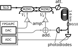
Figure 1: Schematic representation of the experimental system. SLD: superluminescent diode; MZM1 and MZM2: dual input - dual output Mach-Zehnder Modulators; $V_{1}$ and $V_{2}$: driving voltages of the MZMs; att.: programmable optical attenuator; add.: electrical combiner; amp.: pulse amplifier.

Experimental implementation. In the present work we show how Eqs. (2) and (9) can be realised using the same physical setup. Our fibre optics experiment is depicted in Figure 1. Light is generated by a superluminescent diode (SLD) emitting in the telecommunications band (1550 nm, with a 33 nm FWHM), modulated by two dual input / dual output Mach-Zehnder modulators (MZM), and attenuated using a programmable optical attenuator used to control the total loop amplification of the system, i.e. $\mu$ in Eq. (2). It then propagates through an approximately 1.6 km long spool of optical fibre which provides a total loop delay of 7.93 µs. The light is split and enters two photodiodes, one of which provides the feedback signal. The signals are produced and recorded by Digital to Analog Converters (DAC) and Analog to Digital Converters (ADC), controlled by a Xilinx Virtex 6 FPGA chip. The FPGA simultaneously generates the input voltage signals and records the output signals. The FPGA communicates with a PC that controls the whole experiment. (Further details on the experimental setup are given in the Supplementary material).

The key innovation with respect to the earlier experiments Larger et al. (2012); Paquot et al. (2012) is the use of two dual input / dual output MZMs, see Fig. 1, which allows to implement both Eqs. (2) and (9) using the same physical system. Taking into account the incoherence of light in the two branches between the modulators (see Supplementary Material for details), the output of the upper branch of MZM2 (see Fig. 1) can be found to be:

$$I_{2}^{+}=\frac{I_{0}}{2}\left[1+\sin(V_{1}/V_{0})\sin(V_{2}/V_{0})\right],$$ (10)

where $I_{0}$ is the input intensity in the upper branch of MZM1, $V_{1}$ and $V_{2}$ are the driving voltages and $V_{0}$ a constant depending on the MZM. The computational details are presented in the Supplementary Material. In the forward mode, we choose $V_{1}/V_{0}=\pi/2$. The transfer function thus acts as a sinusoidal function for the input argument $V_{2}/V_{0}=a(t)+z(t)$. The constant offset $I_{0}/2$ is removed by the high-pass filter of the amplifier, that drives the MZM. Therefore, once the loop is closed, we end up with Eq. (2). In the backward mode we drive MZM1 with a voltage $V_{1}/V_{0}=a(q)+z(q)+\pi/2$, and MZM2 with a signal proportional to $\bar{e}(q)+e(q)$, but scaled down sufficiently such that $\sin(V_{2}/V_{0})\approx V_{2}/V_{0}=\bar{e}(q)+e(q)$, which gives the desired functionality for the adjoint system Eq. (9).

In order to train our reservoir computer, we first choose a value of $\mu$ close to the threshold for instability. We then iterate the following three steps for (typically) several thousands of iterations, during which performance slowly improves until it converges:

1) We take the training data (typically a small subsequence of the complete set), and convert it to $z(t)$ using the input masks. We feed this signal to the experimental setup, physically implementing Equation 2. Next, we measure and record the signal $a(t)$, and generate an output sequence $y_{i}$ using the output masks.

2) From the output and the desired target values we compute the sequence $e_{i}=\partial C/\partial y_{i}$ at the output, and convert it to $\bar{e}(t)$, now using the output mask as an input mask. Next we time-invert it and feed it back into the experimental setup. Simultaneously we drive the first MZM with the (time-inverted) signal $a(q)+z(q)$ in order to implement the online multiplication with $J(q)$. We record the response signal $e(q)$.

3) From the recorded signals $a(t)$ and $e(t)$ we obtain the gradients for the masking signals, which we use to update the input and output masks:

$$m(r) \leftarrow m(r)-\eta\,{dC}/{dm(r)},$$

$$m_{b}(r) \leftarrow m_{b}(r)-\eta\,{dC}/{dm_{b}(r)},$$

$$u(r) \leftarrow u(r)-\eta\,{dC}/{du(r)},$$

$$u_{b} \leftarrow u_{b}-\eta\,{dC}/{du_{b}},$$ (11)

where $\eta$ is a (typically small) learning rate. In order to speed up convergence we applied a slightly more advanced variant of these update rules known as Nesterov momentum Nesterov (1983); Sutskever et al. (2013) (details are given in the Supplementary material).

Results. We experimentally validate the above scheme using the system described in Fig. 1 by testing it on three time series processing task. We consider first of all the NARMA10 task Atiya and Parlos (2000), an academic task often used in the RC community. Here the input sequence $s_{i}$ consists of a series of independent and identically distributed random numbers drawn uniformly from the interval $\left[0,0.5\right]$. The desired output sequence is given by

$$y^{*}_{i}=0.3y^{*}_{i-1}+0.05y^{*}_{i-1}\sum_{n=1}^{10}{y^{*}_{i-n}}+1.5s_{i}s_{i-9}+0.1.$$

The second task we will call VARDEL5 (from variable delay). Here the input sequence consists of i.i.d. digits drawn from the set $\{1,2,3,4,5\}$. The desired output is then given by $y^{*}_{i}=s_{i-s_{i}}$, i.e., the goal is to retrieve the input instance delayed with the number of time steps given by the current input.

As a performance metric for NARMA10 and VARDEL5 we use the normalised root mean square error (NRMSE), which is given by

$$\text{NRMSE}=\sqrt{\frac{\left<(y_{i}-y^{*}_{i})^{2}\right>_{i}}{\left<(y^{*}_{i})^{2}\right>_{i}}}.$$

The NRMSE varies between 0 (perfect match), and 1 (no relation between output and target).

The third task is a frame-wise phoneme labelling task. We use the TIMIT dataset Garofolo et al. (1993), a speech dataset in which each time step has been labelled with one of 39 phonemes. The input data is high-dimensional (consisting of 39 frequency channels), and the desired output is one of (coincidentally) 39 possible output classes. The goal is to label each frame in a separate test set. Consequently, the performance metric is now the classification error rate, i.e., the fraction of misclassified phonemes in the test set. Note that the masking scheme and BP algorithm is easily extended to multidimensional in – and output sequences (more details are provided in the Supplementary material). The TIMIT task has been studied before in the context of RC, which has shown it to be challenging, typically requiring extremely large reservoirs to obtain competitive performance Triefenbach et al. (2010, 2014).

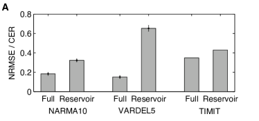
Figure 2: Comparison of performances for the three tasks under consideration. We show either NRMSE (for NARMA10 and VARDEL5) or the classification error rate (CER) for TIMIT. For each task we show performance for a fully trained systems (Full) vs. those trained using the RC paradigm (Reservoir). Error bars indicate standard deviations if available.

For all these tasks we compared performance of the fully trained system to traditional RC, where we kept the input and bias masks fixed and random, and only optimised their global scaling and the feedback strength parameter $\mu$. Full experimental details for each task may be found in the supplementary material, together with an example of optimised input masks and of convergence of NRMSE during training. The results are shown in Figure 2. The experimental setup is successful in performing both useful computations, and implementing its own training process. The fully trained system consistently outperforms the RC approach in all tasks considered.

For the NARMA10 task we improve over all previous experimental results. The previous best was published in Vinckier et al. (2015), which reported an NRMSE of 0.249 for 50 virtual nodes, and 0.22 for 300 virtual nodes, whereas here we obtain a NRMSE of 0.185 for 80 nodes (note that in Vinckier et al. (2015) they report normalised mean square error (NMSE), which is the square of the NRMSE). That result was obtained on an experimental setup that was specially designed to produce a minimal amount of noise (using a passive cavity as a reservoir). The lowest reported experimental NRMSE on a setup equivalent to ours was 0.41 Paquot et al. (2012). Note that we obtain a better average performance for the RC setup ($\text{NRMSE}=0.32$), which is most likely due to the higher number of virtual nodes (80 as opposed to 50 in Paquot et al. (2012)).

For the VARDEL5 task, we cannot directly compare to literature, however as pointed out in chapter 5 of Hermans (2012), this task is an important example of a task that is so nonlinear that it is nearly impossible to solve it with RC. This is confirmed here; the NRMSE of RC is 0.66, indicating that the reservoir has only captured the task on a very rudimentary level. The fully trained system shows a drastically better performance (NRMSE = 0.15). This shows that training the input masks not just allows for better performance on existing tasks, but also allows to tackle tasks that are so intricate that they are considered beyond the reach of traditional RC.

For the TIMIT task we obtain a classification error rate of 34.8% for fully trained systems, vs. 42.9% for the standard RC approach. These results are only slightly worse than similar experimental results presented in Hermans et al. (2015b), (33.2% for fully trained systems and 40.5% for the RC approach) where 600 virtual nodes were used as opposed as 200 in our case.

Discussion. The present work confirms the results anticipated in Hermans et al. (2015a, b): the performance of delay-based reservoir computers can be drastically improved by optimising both input and output masks. Furthermore, following the proposal of Hermans et al. (2015c), we showed that the underlying hardware is capable of running a large part of its own optimisation process. We performed our demonstrations on a fast electro-optical system (whose speed could be readily improved by several orders of magnitude, see, e.g. Brunner et al. (2013)), and on tasks considered hard in the RC community. Importantly, our work has revealed that the BP algorithm is robust against various experimental imperfections (see the Supplementary Material for details), as the performance gains we obtained on all three tasks were similar to those predicted by numerical simulations.

Although our experiment relies on the sine nonlinearity and its cosine derivative, other nonlinear functions can also be successfully realised in hardware with their derivatives. For instance, the so-called linear rectifier function, which truncates the input signal below a certain threshold, is a popular activation function in neural architectures Glorot et al. (2011). Its derivative is a simple binary function which can be easily implemented using an analogue switch, as in Hermans et al. (2015c). In Shi and Lu (2002) it is shown how to implement a sigmoid nonlinearity and its derivative. And in Vandoorne et al. (2014); Vinckier et al. (2015) the nonlinearity is quadratic, and therefore the derivative, which is linear, should also be easy to implement. Furthermore, the BP algorithm is robust against imperfect implementation of the derivative, as shown in section 4.3 of the Supplementary Material, and in the Supplementary Material of Hermans et al. (2015c) (Supplementary Note 4). Therefore we expect that physical implementation of the BP algorithm will be possible in a wide variety of physical systems.

The current setup still requires some slow digital processing to perform the masking and to compute gradients from the recorded signals. Performing masking operations in analog hardware, however, is actively being researched Duport et al. (2016), and these approaches could be used to speed up the present setup. Another limitation is the relatively slow data transfer between the FPGA and the computer. Implementing the full training algorithm on the FPGA would drastically increase the speed of the experiment. FPGA’s have already been demonstrated to be useful for controlling and training electro-optical signal processors Antonik et al. (2015, 2016).

Nowadays, there’s an increased interest in unconventional, neuromorphic computing, as this could allow for energy efficient computing, and may provide a solution to the predicted end of Moore’s law Waldrop (2016). These novel approaches to computing will likely be made with components that exhibit strong element-to-element variability, or whose characteristics evolve slowly with time. Self-learning hardware may be the solution that enables these systems to fulfil their potential. The results in Hermans et al. (2015c) and in this paper therefore constitute an important step towards this goal.