Properties of Surface Plasmon Polaritons on lossy materials: Lifetimes, periods and excitation conditions

Abstract

The possibility to excite Surface Plasmon Polaritons (SPPs) at the interface between two media depends on the optical properties of both media and geometrical aspects. Specific conditions allowing the coupling of light with a plasmon-active interface must be satisfied. Plasmonic effects are well described in noble metals where the imaginary part of the dielectric permittivity is often neglected (“perfect medium approximation”). However, some systems exist for which such approximation cannot be applied, hence requiring a refinement of the common SPP theory. In this context, several properties of SPPs such as excitation conditions, period of the electromagnetic field modulation and SPP lifetime then may strongly deviate from that of the perfect medium approximation. In this paper, calculations taking into account the imaginary part of the dielectric permittivities are presented. The model identifies analytical terms which should not be neglected in the mathematical description of SPPs on lossy materials. These calculations are applied to numerous material combinations resulting in a prediction of the corresponding SPP features. A list of plasmon-active interfaces is provided along with a quantification of the above mentioned SPP properties in the regime where the perfect medium approximation is not applicable.

Keywords: surface plasmon polaritons, lossy materials, plasmon lifetime

1 Introduction

Surface Plasmon Polaritons (SPPs) are collective oscillations of electrons occuring at the interface of materials. More than hundred years after their discovery [1], SPPs have promoted new applications in many fields such as microelectronics [2], photovoltaics [3], near-field sensing [4, 5, 6], laser techonology [7, 8], photonics [9, 10], meta-materials design [11], high order harmonics generation [12], or charged particles acceleration [13, 14].

Most of these applications are based on expensive noble metals such as gold, silver or platinum, as these materials greatly support the plasmonic phenomena, exhibit very small (plasmonic) losses and the experimental results match well with the associated theory [1, 4, 7, 15, 16]. Although there were numerous studies addressing SPPs in lossy materials [17, 18, 19, 20, 21, 22, 23, 24, 25, 26, 27, 28, 29], some specific aspects remain to be investigated.

In this paper, a mathematical condition for SPP excitation at flat interfaces is provided. This approach includes the widely accepted theory but reveals a wider (material dependent) domain of SPP excitation than predicted by the existing literature. The importance of the terms originating from losses is underlined and complemented by formula of the SPP near-field period and lifetime.

2 Excitation conditions for Surface Plasmon Polariton in lossy materials

At a planar interface between two different materials, the electric field components ($E_{x,y,z}$) and magnetic field components ($H_{x,y,z}$) can be calculated by solving the Helmholtz equation for Transverse Magnetic (TM) and Transverse Electric (TE) boundary conditions [1, 16, 30]. For the geometry provided in Fig. 1, the mathematical solutions crucially depend on two complex-valued properties: the dielectric permittivities $\varepsilon_{i}\in\mathbb{C}$ (linked to the optical refractive indices $n_{i}$ of medium $i$ by $\varepsilon_{i}=n_{i}^{2}$), and the complex-valued wavenumbers $k_{i}\in\mathbb{C}$ (associated with electromagnetic field modes in the medium $i$). At the interface between two media (1 and 2), the conservation of light momentum results in the condition [1]

$$k_{1,2}^{2}=\beta^{2}-k_{0}^{2}\varepsilon_{1,2},$$ (1)

where $\beta\in\mathbb{C}$ is the SPP wavenumber along the interface, $k_{0}=\frac{\omega}{c}$ is the wavenumber of the incident light ($\omega\in\mathbb{R}$: light angular frequency, $c$: light velocity in vacuum).

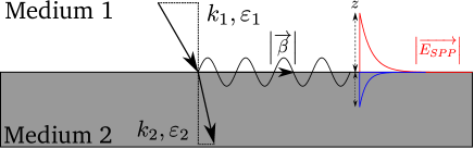
Figure 1: Scheme of a planar interface between medium 1 and 2 at which Surface Plasmon Polaritons are considered. The wavevector components along the surface normal axis are indicated as $k_{1,2}$ and $\varepsilon_{1,2}$ are the complex dielectric permittivities of both media. $\beta$ is the complex wavenumber of the SPPs propagating along the surface plane.

In TM geometry, the continuity conditions for the electromagnetic fields results in the relation [1, 16, 30]

$$\frac{k_{1}}{\varepsilon_{1}}+\frac{k_{2}}{\varepsilon_{2}}=0.$$ (2)

Equation (2) represents the dispersion relation of Surface Plasmon Polaritons at the interface between two semi-infinite media. The signs of $\Re e(k_{1})$ and $\Re e(k_{2})$ were taken positive here, accounting for the exponential decay of the electromagnetic field amplitude in the direction perpendicular to (away from) the interface. The combination of Eqs. (1) and (2) provides the solutions of the SPP wavenumber $\beta$:

$$\beta = \pm\frac{\omega}{c}\sqrt{\frac{\varepsilon_{1}\varepsilon_{2}}{\varepsilon_{1}+\varepsilon_{2}}}.$$ (3)

In order to address the mathematical description of damped surface electromagnetic waves, in the following, we selected the positive branch of $\beta$.

It must noted that in a generalized view, the characterization of lossy waves can be treated by calculating an observable response function $F(\omega,\beta)$ which allows to construct a dispersion relation by locating its complex zeros/poles [21, 23].

As already noted by Ritchie et al. [23], when damping is relevant, the dispersion relation $\omega(\beta)$ for $\beta\in\mathbb{R}$ may have complex solutions ($\omega\in\mathbb{C}$). Conversely, if $\omega$ is real-valued, $\beta$ may be complex-valued. Although straightforward in a theoretical framework, there is some ambiguity about the significance of complex values of $\omega$ or $\beta$ in the interpretation of experiments [23].

In experiments it may be difficult to observe temporal or spatial decay of a resonance due to its rapidity or smallness. The properties of such excitations are usually extracted from the transfer of energy and momentum to the system, involving both real $\omega$ and real $k$. As an example, dispersion relations have been determined by Attenuated Total Reflection (ATR) in Otto configuration [4]. In this approach, a beam is totally reflected at the basis plane of an optical prism. Excitation of SPP in a neighbored metal surface may be realized via coupling through a gap of a dielectric medium (air). SPP manifest as drops in the totally reflected signal, when momentum matching between light and SPP occurs. Experimentally, as underlined by Kovener et al. [21], this can be realized either for a variation of frequency $\omega$ at a fixed angle of incidence $\theta$, or via a variation of $\theta$ at a fixed $\omega$. The first procedure produces dispersion curves with a specific ”bend back” feature, while the second procedure results in curves without that feature [21].

To calculate the excitation conditions of SPPs at the interface between two arbitrary (absorbing) media, a mathematical analysis is presented in the following.

2.1 Sign analysis on the dispersion relation

SPPs can be excited only if the dispersion relation [Eq. (2)] is fulfilled. In order to extract the SPP excitation conditions from the dispersion relation, a sign analysis can be performed on the real and imaginary parts of Eq. (2), which can be mathematically developed to:

$$\cases{\Re e\left(\frac{k_{1}}{\varepsilon_{1}}+\frac{k_{2}}{\varepsilon_{2}}\right)&= 0\\ \Im m\left(\frac{k_{1}}{\varepsilon_{1}}+\frac{k_{2}}{\varepsilon_{2}}\right)&= 0}$$ (4)

By assuming

$$\Re e\left(k_{1}\right)>0\mbox{ and }\Re e\left(k_{2}\right)>0,$$

this equation can be used to deduce a constraint on the sign of real part of the dielectric permittivities $\varepsilon_{1,2}$, resulting in

$$\Re e\left(\frac{\varepsilon_{1}}{\varepsilon_{2}}\right)<0.$$ (5)

Equation (5) defines the first necessary condition for excitation of Surface Plasmon Polaritons, which is equivalent to

$$\Re e\left(\varepsilon_{1}\right)\times\Re e\left(\varepsilon_{2}\right)+\underbrace{\Im m\left(\varepsilon_{1}\right)\times\Im m\left(\varepsilon_{2}\right)}_{\mbox{important for lossy materials}}<0.$$ (6)

The physical meaning of Eq. (6), named Condition 1 for SPP excitation, is the following: in presence of a perfect dielectric medium (e.g. for $\Im m\left(\varepsilon_{1}\right)=0$ or $\Im m\left(\varepsilon_{2}\right)=0$), Eq. (6) implies that SPPs can only be excited at a dielectric - metal interface. This is usually fulfilled when $\Im m\left(\varepsilon_{1,2}\right)\ll\left|\Re e\left(\varepsilon_{1,2}\right)\right|$. Then Eq. (6) reduces to the widely accepted expression [1, 30, 31]

$$\Re e\left(\varepsilon_{1}\right)\times\Re e\left(\varepsilon_{2}\right)<0.$$ (7)

However, in presence of two absorbing media (having then $\Im m\left(\varepsilon_{1}\right)>0$ and $\Im m\left(\varepsilon_{2}\right)>0$), the physical meaning is less intuitive. The condition given by Eq. (6) is more complex due to non-vanishing contributions of the imaginary parts of the dielectric permittivities. Consequences of this additional term, important for lossy materials, will be discussed in Section 2.3.

2.2 Perfect medium approximation and beyond

Assuming purely real-valued dielectric permittivities, Eq. (3) is typically used to derive another condition for SPP excitation. This approach is called Perfect Medium Approximation (PMA) and will be outlined in the following. For simplicity, we adopt the following notations: $\varepsilon_{i}^{\prime}=\Re e\left(\varepsilon_{i}\right)$ and $\varepsilon_{i}^{\prime\prime}=\Im m\left(\varepsilon_{i}\right)$. If $\varepsilon^{\prime\prime}_{1}$ and $\varepsilon^{\prime\prime}_{2}=0$, then $\beta$ is real-valued ($\mathbb{R}$), and Eq. (3) becomes

$$\cases{\Re e\left(\frac{\varepsilon_{1}\varepsilon_{2}}{\varepsilon_{1}+\varepsilon_{2}}\right)>0\\ \Im m\left(\frac{\varepsilon_{1}\varepsilon_{2}}{\varepsilon_{1}+\varepsilon_{2}}\right)=0.}$$ (8)

The latter can be rewritten as

$$\cases{\frac{\left(\varepsilon_{1}^{\prime}\varepsilon_{2}^{\prime}-\varepsilon_{1}^{\prime\prime}\varepsilon_{2}^{\prime\prime}\right)\left(\varepsilon_{1}^{\prime}+\varepsilon_{2}^{\prime}\right)+\left(\varepsilon_{1}^{\prime\prime}\varepsilon_{2}^{\prime}+\varepsilon_{1}^{\prime}\varepsilon_{2}^{\prime\prime}\right)\left(\varepsilon_{1}^{\prime\prime}+\varepsilon_{2}^{\prime\prime}\right)}{\left(\varepsilon_{1}^{\prime}+\varepsilon_{2}^{\prime}\right)^{2}+\left(\varepsilon_{1}^{\prime\prime}+\varepsilon_{2}^{\prime\prime}\right)^{2}}&$>$ 0\\ \frac{\left(\varepsilon_{1}^{\prime\prime}\varepsilon_{2}^{\prime}+\varepsilon_{1}^{\prime}\varepsilon_{2}^{\prime\prime}\right)\left(\varepsilon_{1}^{\prime}+\varepsilon_{2}^{\prime}\right)-\left(\varepsilon_{1}^{\prime}\varepsilon_{2}^{\prime}-\varepsilon_{1}^{\prime\prime}\varepsilon_{2}^{\prime\prime}\right)\left(\varepsilon_{1}^{\prime\prime}+\varepsilon_{2}^{\prime\prime}\right)}{\left(\varepsilon_{1}^{\prime}+\varepsilon_{2}^{\prime}\right)^{2}+\left(\varepsilon_{1}^{\prime\prime}+\varepsilon_{2}^{\prime\prime}\right)^{2}}&= 0}$$

which is strictly equivalent to

$$\frac{\varepsilon_{1}^{\prime}\varepsilon_{2}^{\prime}}{\varepsilon_{1}^{\prime}+\varepsilon_{2}^{\prime}}>0.$$ (9)

Condition [Eq. (9)] implies

$$\left|\varepsilon_{2}^{\prime}\right|>\varepsilon_{1}^{\prime}$$ (10)

and widely used in literature [16, 31]. In particular, when medium 1 is air ($\varepsilon_{1}=1$), the joint application of Eqs. (7) and (10) leads to the well admitted condition

$$\Re e\left(\varepsilon_{2}\right)<-1.$$ (11)

However, beyond the perfect medium approximation, it must be noted that Eq. (3) can be treated using fully complex permittivity values since $\beta$ is defined in $\mathbb{C}$ for any value of the dielectric permittivities $\varepsilon_{i}$. As a consequence, in presence of one (or more) ”lossy” materials, e.g., when $\Im m\left(\varepsilon_{1}\right)>0$ or $\Im m\left(\varepsilon_{2}\right)>0$, there is no other restriction for SPP excitation than the Condition 1 given by Eq. (6). In other words, performing an ad-hoc restriction of the dielectric permittivity to its real part(s) may lead to an oversimplified SPP excitation condition.

2.3 Exploration of plasmon-active material combinations

In this section, the plasmon activity of a wide set of material combinations is explored by comparing predictions of the PMA [real-valued Eqs. (7) and (9)] with the more general case [complex-valued Eq. (6)]. For that, if not stated differently, data of the optical constants were taken from Ref. [32]. Values are listed in A.

In a first step, a selection of different metals exposed to air are analyzed. The results for the SPP-activity for 12 different noble and transition metals are provided in Tab. 1. Here we restrict the study to two wavelengths frequently used in laser processing: 800 nm and 400 nm. However, these calculations can be generalized to other material combinations and wavelengths. The SPP-activity of the metal-air interfaces is indicated by a green tick ($\surd$), whereas the interfaces which do not support SPPs are marked by a red cross ($\times$). At both wavelengths the generalized model [Eq. (6)] predicts similar results as the PMA. Interestingly, and opposed to the PMA, Niobium (Nb) is predicted to support SPPs when interfaced with air, upon 400 nm irradiation.

Interface	$\lambda=800$ nm		$\lambda=400$ nm
	$\Im m\left(\varepsilon_{2}\right)=0$	$\Im m\left(\varepsilon_{2}\right)\neq 0$	$\Im m\left(\varepsilon_{2}\right)=0$	$\Im m\left(\varepsilon_{2}\right)\neq 0$
Air/Ag	$\surd$	$\surd$	$\surd$	$\surd$
Air/Al	$\surd$	$\surd$	$\surd$	$\surd$
Air/Au	$\surd$	$\surd$	$\surd$	$\surd$
Air/Cr	$\surd$	$\surd$	$\surd$	$\surd$
Air/Cu	$\surd$	$\surd$	$\surd$	$\surd$
Air/Fe	$\surd$	$\surd$	$\surd$	$\surd$
Air/Nb	$\surd$	$\surd$	$\times$	$\surd$
Air/Ni	$\surd$	$\surd$	$\surd$	$\surd$
Air/Pt	$\surd$	$\surd$	$\surd$	$\surd$
Air/Ti	$\surd$	$\surd$	$\surd$	$\surd$
Air/V	$\times$	$\times$	$\surd$	$\surd$
Air/W	$\times$	$\times$	$\times$	$\times$

Table 1: Analysis of SPP-activity of several metal ($\varepsilon_{2}$) surfaces irradiated in air ($\varepsilon_{1}=1$) at $\lambda=800$ nm and $400$ nm wavelengths. Meaning of the symbols: ${\color[rgb]{0,0.88,0}\surd}:$ SPP are excited, ${\color[rgb]{1,0,0}\times}$: SPP are not excited at the interface. Bold font indicates interfaces where the prediction deviates from accepted theories.

Interface	$\lambda=800$ nm		$\lambda=400$ nm
	$\Im m\left(\varepsilon_{2}\right)=0$	$\Im m\left(\varepsilon_{2}\right)\neq 0$	$\Im m\left(\varepsilon_{2}\right)=0$	$\Im m\left(\varepsilon_{2}\right)\neq 0$
SiO2/Ag	$\surd$	$\surd$	$\surd$	$\surd$
SiO2/Al	$\surd$	$\surd$	$\surd$	$\surd$
SiO2/Au	$\surd$	$\surd$	$\times$	$\surd$
SiO2/Cr	$\times$	$\surd$	$\surd$	$\surd$
SiO2/Cu	$\surd$	$\surd$	$\surd$	$\surd$
SiO2/Fe	$\surd$	$\surd$	$\surd$	$\surd$
SiO2/Nb	$\surd$	$\surd$	$\times$	$\surd$
SiO2/Ni	$\surd$	$\surd$	$\surd$	$\surd$
SiO2/Pt	$\surd$	$\surd$	$\surd$	$\surd$
SiO2/Ti	$\surd$	$\surd$	$\surd$	$\surd$
SiO2/V	$\times$	$\times$	$\surd$	$\surd$
SiO2/W	$\times$	$\times$	$\times$	$\times$

Table 2: Analysis of SPP-activity of several metal surfaces ($\varepsilon_{2}$) irradiated at $\lambda=800$ nm, and $400$ nm wavelengths through SiO₂ as covering medium [$\varepsilon_{1}($SiO${}_{2},\lambda=800$ nm$)=2.11$, $\varepsilon_{1}($SiO${}_{2},\lambda=400$ nm$)=2.16$]. Meaning of the symbols: ${\color[rgb]{0,0.88,0}\surd}:$ SPP are excited, ${\color[rgb]{1,0,0}\times}$: SPP are not excited at the interface. Bold font indicates interfaces where the prediction deviates from accepted theories.

In a second step, the same metals in contact with a semi-infinite dielectric medium (SiO₂) were addressed. Tab. 2 lists the corresponding results on SPP-activity. Again, with a few exceptions, agreement is found between the PMA and the generalized approach. The case of Nb is similar as in the analysis for air (compare Tabs. 1 and 2). Interestingly, at 400 nm wavelength, the PMA predicts no SPP-activity for the SiO₂/Au interface, while the more general treatment does. Also for SiO₂-covered Cr at 800 nm wavelength, the predictions of both theories do not match.

In a third step, three most relevant metals (Ag, Au, Ti) in contact with a dielectric (air, Al₂O₃, SiO₂, TiO₂, ZnO) or semiconducting (GaAs, GaP, Ge, InP, Si, SiC) medium were analyzed regarding their SPP-activity at 800 nm and 400 nm wavelengths. Tab. 3 compiles the corresponding information and indicates that for Au and Ag at 800 nm, both models provide the same predictions on SPP-activity. However, for Ti at 800 nm and for all three metals at 400 nm, differences between predictions of both models can be observed. For Ti, the differences between those models arise for the significant contribution of the imaginary part of the dielectric permittivity [see Eq. (6), $\varepsilon_{2}(\mathrm{Ti},\lambda=800$ nm$)=-2.85+i19.11$, $\varepsilon_{2}(\mathrm{Ti},\lambda=400$ nm$)=-2.22+i6.66$]. For Au and Ag at 400 nm wavelength, the different model predictions arise from a similar origin (see Table 4).

Interface	$\lambda=800$ nm		$\lambda=400$ nm
	$\Im m\left(\varepsilon_{2}\right)=0$	$\Im m\left(\varepsilon_{2}\right)\neq 0$	$\Im m\left(\varepsilon_{2}\right)=0$	$\Im m\left(\varepsilon_{2}\right)\neq 0$
Air/Ag	$\surd$	$\surd$	$\surd$	$\surd$
Al2O3/Ag	$\surd$	$\surd$	$\surd$	$\surd$
GaAs/Ag	$\surd$	$\surd$	$\times$	$\surd$
GaP/Ag	$\surd$	$\surd$	$\times$	$\surd$
Ge/Ag	$\surd$	$\surd$	$\times$	$\surd$
InP/Ag	$\surd$	$\surd$	$\times$	$\surd$
Si/Ag	$\surd$	$\surd$	$\times$	$\surd$
SiC/Ag	$\surd$	$\surd$	$\times$	$\surd$
SiO2/Ag	$\surd$	$\surd$	$\surd$	$\surd$
TiO2/Ag	$\surd$	$\surd$	$\times$	$\surd$
ZnO/Ag	$\surd$	$\surd$	$\times$	$\surd$
Air/Au	$\surd$	$\surd$	$\surd$	$\surd$
Al2O3/Au	$\surd$	$\surd$	$\times$	$\surd$
GaAs/Au	$\surd$	$\surd$	$\times$	$\times$
GaP/Au	$\surd$	$\surd$	$\times$	$\surd$
Ge/Au	$\surd$	$\surd$	$\times$	$\times$
InP/Au	$\surd$	$\surd$	$\times$	$\times$
Si/Au	$\surd$	$\surd$	$\times$	$\surd$
SiC/Au	$\surd$	$\surd$	$\times$	$\surd$
SiO2/Au	$\surd$	$\surd$	$\times$	$\surd$
TiO2/Au	$\surd$	$\surd$	$\times$	$\surd$
ZnO/Au	$\surd$	$\surd$	$\times$	$\surd$
Air/Ti	$\surd$	$\surd$	$\surd$	$\surd$
Al2O3/Ti	$\surd$	$\surd$	$\surd$	$\surd$
GaAs/Ti	$\times$	$\surd$	$\times$	$\times$
GaP/Ti	$\times$	$\surd$	$\times$	$\surd$
Ge/Ti	$\times$	$\surd$	$\times$	$\times$
InP/Ti	$\times$	$\surd$	$\times$	$\times$
Si/Ti	$\times$	$\surd$	$\times$	$\surd$
SiC/Ti	$\times$	$\surd$	$\times$	$\surd$
SiO2/Ti	$\surd$	$\surd$	$\surd$	$\surd$
TiO2/Ti	$\times$	$\surd$	$\times$	$\surd$
ZnO/Ti	$\surd$	$\surd$	$\times$	$\surd$

Table 3: Analysis of SPP-activity of three metal surfaces (Ag, Au, Ti) irradiated through different dielectric or semiconducting media at $\lambda=800$ nm and $400$ nm wavelengths. Meaning of the symbols: ${\color[rgb]{0,0.88,0}\surd}:$ SPP are excited, ${\color[rgb]{1,0,0}\times}$: SPP are not excited at the interface. Bold font indicates interfaces where the prediction deviates from accepted theories.

3 Period of Surface Plasmon Polaritons in lossy materials

3.1 Modeling the plasmon period

The spatial period $\Lambda$ of the electromagnetic field can be calculated from the complex-valued SPP wavenumber $\beta$ [using Eq. (3)] via [17, 33]

$$\Lambda=\frac{2\pi}{\Re e\left(\beta\right)},$$ (12)

with

$$\Re e\left(\beta\right)=\frac{\omega}{2c}\,\sqrt{2\,\left[F_{1}^{2}+F_{2}^{2}\right]^{1/2}+2F_{1}},$$

where

$$F_{1}=\left(\varepsilon_{1}^{\prime}\varepsilon_{2}^{\prime}\underbrace{-\varepsilon_{1}^{\prime\prime}\varepsilon_{2}^{\prime\prime}}\right)\left(\varepsilon_{1}^{\prime}+\varepsilon_{2}^{\prime}\right)F_{0}+\underbrace{\left(\varepsilon_{1}^{\prime\prime}\varepsilon_{2}^{\prime}+\varepsilon_{1}^{\prime}\varepsilon_{2}^{\prime\prime}\right)\left(\varepsilon_{1}^{\prime\prime}+\varepsilon_{2}^{\prime\prime}\right)F_{0}},$$

$$F_{2}=\underbrace{\left(\varepsilon_{1}^{\prime\prime}\varepsilon_{2}^{\prime}+\varepsilon_{1}^{\prime}\varepsilon_{2}^{\prime\prime}\right)\left(\varepsilon_{1}^{\prime}+\varepsilon_{2}^{\prime}\right)F_{0}-\left(\varepsilon_{1}^{\prime}\varepsilon_{2}^{\prime}-\varepsilon_{1}^{\prime\prime}\varepsilon_{2}^{\prime\prime}\right)\left(\varepsilon_{1}^{\prime\prime}+\varepsilon_{2}^{\prime\prime}\right)F_{0}},$$

and $F_{0}=\left[\left(\varepsilon_{1}^{\prime}+\varepsilon_{2}^{\prime}\right)^{2}\underbrace{+\left(\varepsilon_{1}^{\prime\prime}+\varepsilon_{2}^{\prime\prime}\right)^{2}}\right]^{-1}$. The terms underlined with a curly brackets can be neglected if the PMA is used, i.e., if $\varepsilon^{\prime\prime}_{1}=0$ and $\varepsilon^{\prime\prime}_{2}=0$. From Eq. (12), it is obvious that the imaginary parts of both media can significantly affect the SPP periods.

For the PMA ($\varepsilon^{\prime\prime}_{1}=0$ and $\varepsilon^{\prime\prime}_{2}=0$), Eq. (12) reduces to the expression [31]

$$\Lambda_{\mathrm{PMA}}=\frac{2\pi}{\Re e(\beta)}=\frac{\lambda}{\sqrt{\frac{\varepsilon^{\prime}_{1}\varepsilon^{\prime}_{2}}{\varepsilon^{\prime}_{1}+\varepsilon^{\prime}_{2}}}}.$$ (13)

However, it should be underlined that Eq. (13) should not be applied to lossy materials.

3.2 Exploration of plasmon-active material combinations

In this section, different SPP-active combinations of materials are systematically explored in terms of their SPP period using Eq. (12).

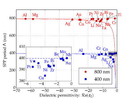
Figure 2: SPP period for several metals irradiated in air at 800 nm (red circles) and 400 nm (blue squares) wavelengths calculated with Eq. (12). The entities $\Lambda=\lambda$ are shown as horizontal dashed lines for both wavelengths. The solid lines represent the periods calculated using the PMA [Eq. (13)]. The inset displays a magnification of the area marked by the grey rectangle.

Fig. 2 shows for metals being SPP-active in air the spatial period $\Lambda$ as a function of their real parts of $\varepsilon_{2}$. At 800 nm wavelength, the SPP-periods calculated by Eq. (12) (discrete data points) match within $5\%$ to the irradiation wavelength $\lambda$ - as indicated by a horizontal red dashed line. The solution based on the PMA (Eq. 13) with $\varepsilon_{1}=1$ is shown as red solid line. By comparison, it is obvious that the PMA (Eq. 13) should not be applied to lossy materials. At 400 nm wavelength, the SPP-periods more strongly depend on the material. A reduction of $\Lambda$ by up to $25\%$, when compared to the wavelength $\lambda$, is observed for Ag, Li, and Na - see the blue horizontal dashed line, with a similar mismatch to the PMA curve (blue solid line).

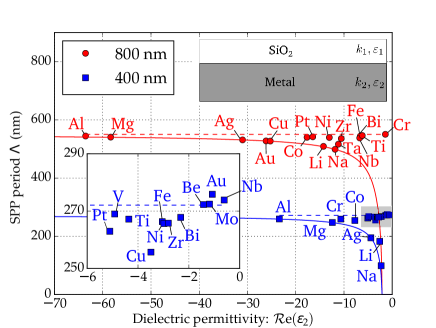
Figure 3: SPP period for several metals irradiated through SiO₂ ($\varepsilon_{1}$) at 800 nm (red circles) and 400 nm (blue squares) wavelengths calculated with Eq. (12). The entities $\Lambda=\lambda/\Re e\sqrt{\varepsilon_{1}}$ are shown as horizontal dashed lines for both wavelengths. The solid lines represent the periods calculated using the PMA [Eq. (13)] with a fixed $\varepsilon_{1}$. The inset displays a magnification of the area marked by the grey rectangle.

Fig. 3 shows the results of analogous analyses for SPP-active metals ($\varepsilon_{2}$) in contact with SiO₂ ($\varepsilon_{1}$). At 800 nm wavelength, the SPP-periods match within $8\%$ to the wavelength in SiO₂ (i.e., above the metal surface, $\lambda/\Re e\sqrt{\varepsilon_{1}}$) [34] - as indicated by a horizontal red dashed line. At 400 nm wavelength, for most metals, the deviations from the latter expression also stay below $10\%$ (compared to the horizontal blue dashed line). In contrast, for Ag, Li and Na, larger differences up to $65\%$ are evident. For both wavelengths, the data points and the periods calculated using the PMA [Eq. (13), solid lines] match only for specific materials.

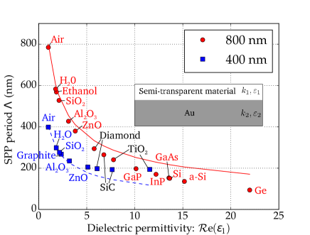
Figure 4: SPP period for Au irradiated through various types of semi-transparents materials at 800 nm (red circles) or 400 nm (blue squares) wavelengths. The entities $\Lambda=\lambda/\Re e\sqrt{\varepsilon_{1}}$ are shown as lines for both wavelengths.

In order to understand the role of the overlayer, the SPP-period is investigated at the interface between Au ($\varepsilon_{2}$) and various semi-transparent materials ($\varepsilon_{1}$). The results are provided in Fig. 4. They indicate that, again, the SPP-periods strongly depends on $\varepsilon_{1}$. Specifically, a reasonably good agreement is found between the SPP-period $\Lambda$ and the wavelength in the covering medium $\lambda/\Re e\sqrt{\varepsilon_{1}}$. This can be seen by the red solid ($\lambda=800$ nm) and blue dashed ($\lambda=400$ nm) lines, which quantitatively agree with the data points for small values of $\Re e(\varepsilon_{1})$. The remarkable deviations at larger values of $\Re e(\varepsilon_{1})$ arise from the PMA.

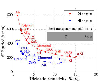
Figure 5: SPP period for Ti irradiated through various types of semi-transparents materials at 800 nm (red circles) or 400 nm (blue squares) wavelengths. The entities $\Lambda=\lambda/\Re e\sqrt{\varepsilon_{1}}$ are shown as lines for both wavelengths.

Fig. 5 shows analogous results for the case of a Ti substrate ($\varepsilon_{2}$) covered by the same set of materials ($\varepsilon_{1}$). Again, the lines represent the wavelengths in the covering medium $\lambda/\Re e\sqrt{\varepsilon_{1}}$, which are in reasonable agreement with the data points.

It should be underlined that the conclusions drawn in this work strongly depend on the quality of the optical data used. All parameters affecting the dielectric permittivities may influence the predictions, i.e., the temperature [35], high-intensity illumination [36, 37, 38], strong external fields, etc. Moreover, we have assumed that the SPP-active interface is surrounded by two semi-infinite half-spaces. This assumption may break down when additional interfaces fall within the vertical extend of SPP field. Then another model has to be used which considers the coherent coupling of SPP at several interfaces [20, 39].

4 Lifetime of Surface Plasmon Polaritons in lossy materials

So far, we have described the Surface Plasmon Polaritons within the frame of steady-state conditions. Once the driving external radiation field is turned off, the SPPs may exist for a certain duration called lifetime $\tau_{\mbox{\small SPP}}$ in the following. Upon internal damping, via electron collisions, re-radiation of light to the far field [40] via scattering on defects, etc., SPP typically vanish on a sub-picosecond timescale. However, the exact lifetime strongly depends on the material and irradiation parameters.

In this section, two different models of SPP lifetime are introduced and applied to the materials Ag and Ti in a wide range of irradiation wavelengths (from UV to IR). Two different models from literature will be compared [16, 41].

The SPP propagation length $L_{SPP}$ ($1/e$-decay of the intensity) is defined by [41]

$$L_{SPP}:=[2\times\Im m{(\beta)}]^{-1}.$$ (14)

Using the group velocity ($v_{g}$) and the lifetime ($\tau_{SPP}$) of SPPs, their propagation length can be approximated by:

$$L_{SPP}\sim v_{g}\times\tau_{SPP}$$ (15)

The group velocity is given by the definition

$$v_{g}:=\frac{d\omega}{d[\Re e(\beta)]}=\frac{c}{n_{SP}(\lambda)-\lambda\frac{dn_{SP}}{d\lambda}}$$ (16)

with $n_{SP}(\lambda)=\Re e\sqrt{\frac{\varepsilon_{1}(\lambda)\varepsilon_{2}(\lambda)}{\varepsilon_{1}(\lambda)+\varepsilon_{2}(\lambda)}}$ [41, 42].

Combining Eqs. (14)-(16) results in an SPP lifetime of

$$\tau_{SPP}\sim\frac{1}{2\times\Im m(\beta)\times v_{g}}.$$ (17)

Another expression of the SPP lifetime was provided by Raether [16] to be:

$$\tau_{SPP}=\frac{1}{2\times\Im m\left(\omega_{SPP}\right)},$$ (18)

where

$$\Im m\left(\omega_{SPP}\right)=\frac{c}{2}\times\frac{\Re e\left(\beta\right)\Im m\left(\epsilon_{2}\right)}{\Re e\left(\varepsilon_{2}\right)^{2}}\times\frac{\Re e\left(\varepsilon_{1}\right)\Re e(\varepsilon_{2})}{\Re e\left(\varepsilon_{1}\right)+\Re e(\varepsilon_{2})}.$$ (19)

In the following two subsections, we apply and compare the two Eqs. (17) and (18) to the well-known case of air-Ag interface (Example 1, a material properly described by the PMA) and the less studied air-Ti interface (Example 2, representing a lossy material).

Example 1 (”lossless” material): air - Ag interface

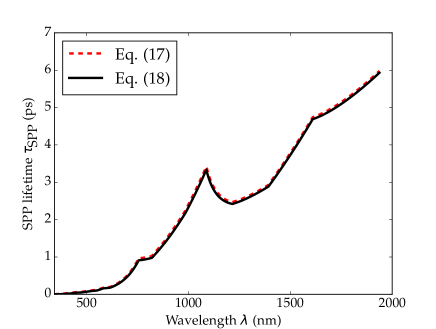
Figure 6: SPP lifetime $\tau_{\mbox{\small SPP}}$ at the air - Ag interface as a function of the irradiation wavelength $\lambda$. Eqs. (17) and (18) were used to compute the red dashed and black solid lines, respectively.

Figure 6 presents the SPP lifetime $\tau_{\mbox{\small SPP}}$ as a function of the irradiation wavelength $\lambda$ (350 nm - 2 $\mu$m). The two curves shown in Fig. 6 are based on Eqs. (17) and (18) along with the optical data from Ref. [43]. Both curves exhibit an excellent agreement featuring lifetimes up to 6 ps. At 400 nm wavelength, $\tau_{\mbox{\small SPP}}$ accounts to 14 fs [Eq. (18)] and 27 fs [Eq. (17)], while at 800 nm wavelength, both equations provide a very similar value of 1 ps. At 400 nm wavelength, $\tau_{\mbox{\small SPP}}$ agrees reasonably well with the experiments of Kubo et al. [44] who observed the SPP decay within 50 fs for the air-Ag interface. It should be underlined that the SPP lifetime strongly depends on the irradiation wavelength, varying by more than two orders of magnitude here.

Example 2 (lossy material): air - Ti interface

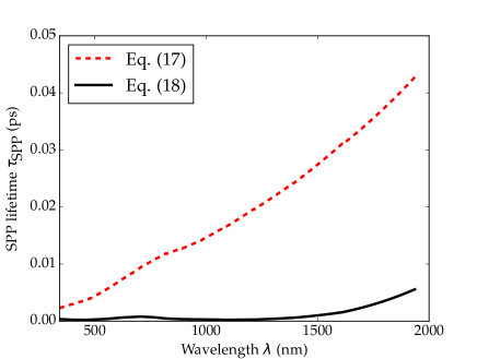
Figure 7: SPP lifetime $\tau_{\mbox{\small SPP}}$ at the air - Ti interface as a function of the irradiation wavelength $\lambda$. Eqs. (17) and (18) were used to compute the red dashed and black solid lines, respectively.

Figure 7 displays the SPP lifetime $\tau_{\mbox{\small SPP}}$ at the air - Ti interface, as a function of the irradiation wavelength $\lambda$. Again, the two curves shown in Fig. 7 are calculated from Eqs. (17) and (18) using the optical data from Ref. [43]. In contrast to Example 1 (Ag), the two curves are remarkably different for the air-Ti interface. The model based on Eq. (18) provides values which are smaller by more than one order of magnitude when compared to the ones provided by Eq. (17). Specifically, at 400 nm wavelength, $\tau_{\mbox{\small SPP}}$ accounts to $0.3$ fs [Eq. (18)] versus $3$ fs [Eq. (17)]. At 800 nm wavelength, it accounts to $0.5$ fs [Eq. (18)] versus $11$ fs [Eq. (17)]. The values calculated by Eq. (18) appear unreasonably small here, as they are smaller than the expected Drude relaxation time of the electrons [45]. It is important to emphasize that the two models result in very different predictions for Ti.

5 Conclusion

In this work, the properties of Surface Plasmon Polaritons at the interface between two lossy materials have been studied. Our mathematical analysis allowed to identify terms which should not be neglected in the mathematical description of SPPs on lossy materials. This rigorous approach was applied to numerous material combinations (dielectric/metal, semiconductor/metal), providing a generalized criterion for SPP excitation along with the quantification of the SPP periods. For Ag and Ti surfaces interfaced with air, the lifetimes of the SPP were reported in a wide spectral range between 350 nm and 2 $\mu$m wavelength pointing out again that plasmonic loss mechanisms should be carefully taken into consideration.

References

Appendix A Optical constants of materials

In this work, several sources of optical data were used. For Al₂O₃, Al, Au, Be, a-C, Co, Cr, Cu, diamond, Ethanol, Fe, GaAs, GaP, Ge, Graphite, H₂O, InP, Li, Mo, Na, Nb, Ni, Pt, c-Si, a-Si, SiC, SiO₂, Ta, Ti, TiO₂, V, and W, the optical data were mostly taken from Ref. [32]. For Mg, the work of Hagemann et al. was used. [46] For ZnO, the work of Postava et al. [32]. The detailed optical data used in this work are summarized in Tab. 4.

Material	Wavelength				Reference
	800 nm		400 nm
	$\Re e\left(\varepsilon\right)$	$\Im m\left(\varepsilon\right)$	$\Re e\left(\varepsilon\right)$	$\Im m\left(\varepsilon\right)$
Air	1.00	0.00	1.00	0.00	-
Ag	-27.95	1.52	-3.77	0.67	[43]
Al2O3	3.10	0.00	3.19	0.00	[32]
Al	-63.55	47.31	-23.39	4.77	[32]
Au	-26.15	1.85	-1.08	6.49	[32]
Be	0.17	23.22	-1.42	18.11	[32]
Bi	-6.61	21.08	-2.32	6.76	[46]
a-C	4.80	3.37	3.53	3.77	[32]
Co	-17.65	25.20	-7.74	7.63	[32]
Cr	-1.42	36.29	-10.65	10.76	[32]
Cu	-25.27	2.52	-3.49	5.22	[32]
Diamond	5.77	0.00	6.08	0.00	[32]
Ethanol	1.84	0.00	-	-	[47]
Fe	-6.38	20.19	-3.05	8.27	[32]
GaAs	13.55	0.63	14.53	18.76	[32]
GaP	10.13	0.00	17.53	2.31	[32]
Ge	21.96	3.01	12.24	18.34	[32]
Graphite	5.95	11.58	5.20	6.76	[32]
H2O	1.76	0.00	1.82	0.00	[32]
InP	11.93	1.46	16.49	15.30	[32]
Li	-14.25	2.16	-2.58	0.96	[32]
Mo	2.08	24.52	-1.19	19.51	[32]
Mg	-58.35	11.33	-12.41	1.25	[46]
Na	-11.84	0.35	-2.30	0.21	[32]
Nb	-6.74	14.49	-0.61	12.90	[32]
Ni	-13.04	21.73	-2.98	7.60	[32]
Pt	-16.47	28.11	-5.11	9.77	[32]
a-Si	15.17	0.85	13.39	18.84	[32]
Si	13.63	0.048	30.85	4.30	[32]
SiC	6.78	0.00	7.64	0.00	[32]
SiO2	2.11	0.00	2.16	0.00	[32]
Ta	-11.17	7.90	2.49	12.60	[32]
Ti	-6.21	25.2	-4.36	12.36	[43]
TiO2	7.78	0.00	11.55	0.00	[32]
V	1.88	21.76	-4.92	17.24	[32]
W	5.22	19.44	5.68	16.34	[32]
ZnO	3.80	0.00	5.11	0.07	[48]
Zr	-10.56	16.38	-2.81	7.18	[49]

Table 4: Summary of the dielectric permittivities used in this work.

References

- [1] S. A. Maier, Plasmonics, Fundamentals and Applications, Springer, 2007.
- [2] K. F. MacDonald, Z. L. Samson, M. I. Stockman, N. I. Zheludev, Ultrafast active plasmonics, Nat. Photonics 3 (1) (2009) 55–58.
- [3] H. A. Atwater, A. Polman, Plasmonics for improved photovoltaic devices, Nat. Mater. 9 (2010) 205–213.
- [4] A. Otto, Experimental investigation of surface polaritons on plane interfaces, in: Festkörperprobleme 14, Springer, 1974, pp. 1–37.
- [5] R. J. Bell, R. W. A. Jr., C. Ward, I. L.Tyler, Introductory theory for surface electromagnetic wave spectroscopy, Surf. Sci. 48 (1975) 253–287.
- [6] A. Kabashin, P. Evans, S. Pastkovsky, W. Hendren, G. Wurtz, R. Atkinson, R. Pollard, V. Podolskiy, A. Zayats, Plasmonic nanorod metamaterials for biosensing, Nat. Mater. 8 (2009) 867–871.
- [7] P. Berini, I. De Leon, Surface plasmon polariton amplifiers and lasers, Nat. Photonics 6 (1) (2011) 16–24.
- [8] I.-Y. Park, S. Kim, J. Choi, D.-H. Lee, Y.-J. Kim, M. F. Kling, M. I. Stockman, S.-W. Kim, Plasmonic generation of ultrashort extreme-ultraviolet light pulses, Nat. Photonics 5 (11) (2011) 677–681.
- [9] W. Barnes, A. Dereux, T. Ebbesen, Surface plasmon subwavelength optics, Nature 424 (2003) 824–830.
- [10] H. Liu, P. Lalanne, Microscopic theory of the extraordinary optical transmission, Nature 452 (7188) (2008) 728–731.
- [11] V. M. Shalaev, Optical negative-index metamaterials, Nat. Photonics 1 (2007) 41–48.
- [12] S. Kim, J. Jin, Y.-J. Kim, I.-Y. Park, Y. Kim, S.-W. Kim, High-harmonic generation by resonant plasmon field enhancement, Nature 453 (7196) (2008) 757–760.
- [13] P. Genevet, J.-P. Tetienne, E. Gatzogiannis, R. Blanchard, M. A. Kats, M. O. Scully, F. Capasso, Large Enhancement of Nonlinear Optical Phenomena by Plasmonic Nanocavity Gratings, Nano Lett. 10 (12) (2010) 4880–4883.
- [14] M. A. Purvis, V. N. Shlyaptsev, R. Hollinger, C. Bargsten, A. Pukhov, A. Prieto, Y. Wang, B. M. Luther, L. Yin, S. Wang, J. J. Rocca, Relativistic plasma nanophotonics for ultrahigh energy density physics, Nat. Photonics 7 (10) (2013) 796–800.
- [15] R. B. Pettit, J. Silcox, R. Vincent, Measurement of surface-plasmon dispersion in oxidized aluminum films, Phys. Rev. B 11 (8) (1975) 3116.
- [16] H. Raether, Surface Plasmons on Smooth and Rough Surfaces and on Gratings, Springer-Verlag, 1986.
- [17] R. J. Bell, R. W. Alexander, W. F. Parks, G. Kovener, Surface excitations in absorbing media, Opt. Commun. 8 (2) (1973) 147.
- [18] R. W. Alexander, G. S. Kovener, and R. J. Bell, Dispersion curves for surface electromagnetic waves with damping, Phys. Rev. Lett. 32, 154 (1974).
- [19] C. A. Ward, R. J. Bell, R. W. Alexander, G. S. Kovener, I. Tyler, Surface electromagnetic waves on metals and polar insulators: some comments, Appl. Opt. 13 (10) (1974) 2378–2381.
- [20] C. A. Ward, R. W. Alexander, R. J. Bell, Surface electromagnetic waves on layered systems with damping, Phys. Rev. B 12 (8) (1975) 3293.
- [21] G. S. Kovener, R. W. Alexander Jr, R. J. Bell, Surface electromagnetic waves with damping. I. Isotropic media, Phys. Rev. B 14 (4) (1976) 1458.
- [22] G. S. Kovener, R. W. Alexander Jr, I. L. Tyler, R. J. Bell, Surface electromagnetic waves with damping. II. Anisotropic media, Phys. Rev. B 15 (12) (1977) 5877.
- [23] R. H. Ritchie, R. N. Hamm, M. W. Williams, and E. T. Arakawa, Dispersion relations of elementary excitations when damping is present, Phys. Status Solidi 84 (1977) 367.
- [24] J. Laglois, B. Fischer, Dispersion theory of surface-exciton polaritons, Phys. Rev. B 17 (1978) 3814.
- [25] R. Reinisch, Theory of nonlinear excitation of surface polaritons in lossy media, Surf. Sci. 85 (1979) 432–456.
- [26] A. D. Boardman, P. Egan, The influence of collisional damping on surface plasmon-polariton dispersion, J. Phys. Colloques 45 (C5) (1984) 179–190.
- [27] A. Norrman, T. Setälä, and A. T. Fridberg, Exact surface-plasmon polariton solutions at a lossy interface, Opt. Lett. 38 (2013) 7.
- [28] H.-I. Lee and J. Mok, Electromagnetic-energy conservation for media with metallic constituents with special attention to damped waves, J. Opt. 15 (2013) 035002.
- [29] R. Martinez-Herrero, A. Garcia-Ruiz, and A. Manjavacas, Parametric characterization of surface plasmon polaritons at a lossy interface, Opt. Express 23 (2015) 28574–28583.
- [30] A. Zayats, I. Smolyaninoy, A. Maradudin, Nano-optics of surface plasmon polaritons, Phys. Rep. 408 (2005) 131–314.
- [31] A. M. Bonch-Bruevich, M. N. Libenson, V. S. Makin, V. A. Trubaev, Surface electromagnetic waves in optics, Opt. Eng. 31 (4) (1992) 718–730.
- [32] E. D. Palik, Handbook of Optical Constants of Solids, Academic Press, 1985.
- [33] A. Ionin, S. Kudryashov, S. Makarov, A. Rudenko, P. Saltuganov, L. Seleznev, D. Sinitsyn, E. Sunchugasheva, Femtosecond laser fabrication of sub-diffraction nanoripples on wet al surface in multi-filamentation regime: High optical harmonics effects?, Appl. Surf. Sci. 292 (2014) 678–681.
- [34] A. E. Siegman, P. M. Fauchet, Stimulated Wood’s anomalies on laser-illuminated surfaces, IEEE J. Quantum Electron. QE-22 (1986) 1384.
- [35] H. H. Landolt, R. Börnstein, Landolt - Börnstein Numerical Data and Functional Relationships, Springer-Verlag.
- [36] J. Bonse, A. Rosenfeld, J. Krüger, On the role of surface plasmon polaritons in the formation of laser-induced periodic surface structures upon irradiation of silicon by femtosecond-laser pulses, J. Appl. Phys. 106 (2009) 104910.
- [37] T. J.-Y. Derrien, T. E. Itina, R. Torres, T. Sarnet, M. Sentis, Possible surface plasmon polariton excitation under femtosecond laser irradiation of silicon, J. Appl. Phys. 114 (2013) 083104.
- [38] E. Bévillon, J. P. Colombier, V. Recoules, H. Zhang, C. Li, R. Stoian, Ultrafast Surface Plasmonic Switch in Non-Plasmonic Metals, Phys. Rev. B 93 (2016) 165416.
- [39] T. J.-Y. Derrien, R. Koter, J. Krüger, S. Höhm, A. Rosenfeld, J. Bonse, Plasmonic formation mechanism of periodic 100-nm-structures upon femtosecond laser irradiation of silicon in water, J. Appl. Phys. 116 (7) (2014) 074902.
- [40] R. Müller, J. Bethge, Plasmonic decay in a metallic grating after femtosecond pulse excitation, Phys. Rev. B 82 (2010) 115408.
- [41] A. Hohenau, A. Drezet, M. Weissenbacher, F. R. Aussenegg, and J. R. Krenn, Effects of damping on surface-plasmon pulse propagation and refraction, Phys. Rev. B 78 (2008) 155405.
- [42] J. D. Jackson, Classical Electrodynamics, 3rd Edition, Wiley, 1999.
- [43] P. B. Johnson, R.-W. Christy, Optical constants of the noble metals, Phys. Rev. B 6 (12) (1972) 4370.
- [44] A. Kubo, K. Onda, H. Petek, Z. Sun, Y. S. Jung, H. K. Kim, Femtosecond imaging of surface plasmon dynamics in a nanostructured silver film, Nano Lett. 5 (6) (2005) 1123–1127.
- [45] M. A. Ordal, R. J. Bell, R. W. A. Jr., L. L. Long, M. R. Querry, Optical properties of fourteen metals in the infrared and far infrared: Al, Co, Cu, Au, Fe, Pb, Mo, Ni, Pd, Pt, Ag, Ti, V, and W, Appl. Opt. 24 (1985) 4493–4499.
- [46] H.-J. Hagemann, W. Gudat, C. Kunz, Optical constants from the far infrared to the x-ray region: Mg, Al, Cu, Ag, Au, Bi, C, and A12O3, J. Opt. Soc. Am. B 65 (6) (1975) 742–744.
- [47] S. Kedenburg, M. Vieweg, T. Gissibl, H. Giessen, Linear refractive index and absorption measurements of nonlinear optical liquids in the visible and near-infrared spectral region, Opt. Mater. Express 2 (11) (2012) 1588–1611.
- [48] K. Postava, H. Sueki, M. Aoyama, T. Yamaguchi, C. Ino, Y. Igasaki, M. Horie, Spectroscopic ellipsometry of epitaxial ZnO layer on sapphire substrate, J. Appl. Phys. 87 (11) (2000) 7820.
- [49] S. Krishnan, C. D. Anderson, P. C. Nordine, Optical properties of liquid and solid zirconium, Phys. Rev. B 49 (5) (1994) 3161.