Characterising the evolving $K$-band luminosity function using the UltraVISTA, CANDELS and HUDF surveys

Abstract

We present the results of a new study of the $K$-band galaxy luminosity function (KLF) at redshifts $z\leq 3.75$, based on a nested combination of the UltraVISTA, CANDELS and HUDF surveys. The large dynamic range in luminosity spanned by this new dataset ($3-4$ dex over the full redshift range) is sufficient to clearly demonstrate for the first time that the faint-end slope of the KLF at $z\geq 0.25$ is relatively steep ($-1.3\leq\alpha\leq-1.5$ for a single Schechter function), in good agreement with recent theoretical and phenomenological models. Moreover, based on our new dataset we find that a double Schechter function provides a significantly improved description of the KLF at $z\leq 2$. At redshifts $z\geq 0.25$ the evolution of the KLF is remarkably smooth, with little or no evolution evident at faint ($M_{K}\geq-20.5$) or bright magnitudes ($M_{K}\leq-24.5$). Instead, the KLF is seen to evolve rapidly at intermediate magnitudes, with the number density of galaxies at $M_{K}\simeq-23$ dropping by a factor of $\simeq 5$ over the redshift interval $0.25\leq z\leq 3.75$. Motivated by this, we explore a simple description of the evolving KLF based on a double Schechter function with fixed faint-end slopes ($\alpha_{1}=-0.5$, $\alpha_{2}=-1.5$) and a shared characteristic magnitude ($M_{K}^{\star}$). According to this parameterisation, the normalisation of the component which dominates the faint-end of the KLF remains approximately constant, with $\phi^{\star}_{2}$ decreasing by only a factor of $\simeq 2$ between $z\simeq 0$ and $z\simeq 3.25$. In contrast, the component which dominates the bright end of the KLF at low redshifts evolves dramatically, becoming essentially negligible by $z\simeq 3$. Finally, we note that within this parameterisation, the observed evolution of $M_{K}^{\star}$ between $z\simeq 0$ and $z\simeq 3.25$ is entirely consistent with $M_{K}^{\star}$ corresponding to a constant stellar mass of $M_{\star}\simeq 5\times 10^{10}\mathrm{M_{\odot}}$ at all redshifts.

1 Introduction

As a basic statistical measurement of the galaxy population, the galaxy luminosity function remains a simple, yet powerful tool for differentiating between competing models of galaxy evolution. In particular, due to its relative insensitivity to dust reddening and strong correlation with stellar mass, it has long been recognised that the near-IR luminosity function provides an insight into the assembly of the underlying stellar mass, without being significantly biased by recent star formation episodes.

Initial studies of the local $K$-band luminosity function (KLF) were undertaken in the 1990s, thanks to the rapid developments in near-IR detector technology, but were confined to samples of a few hundred galaxies selected from relatively small areas of sky (e.g. Mobasher, Sharples & Ellis 1993; Glazebrook et al. 1995; Gardner et al. 1997; Loveday 2000). This restriction was removed with the arrival of the Two Micron All Sky Survey (2MASS; Jarrett et al. 2000). Kochanek et al. (2001) measured the local KLF based on a spectroscopically complete 2MASS sample consisting of 3878 galaxies selected over an area of $\simeq 7000$ deg². Contemporaneously, Cole et al. (2001) measured the local KLF to fainter magnitudes using a spectroscopic sample of 5683 galaxies within a $\simeq 600$ deg² area of overlap between 2MASS and the 2dF galaxy redshift survey (2dFGRS; Colless et al. 2001). The results of the Kochanek et al. (2001) and Cole et al. (2001) studies are fully consistent and, after conversion to our adopted cosmology, indicated that the local KLF could be reasonably well described by a single Schechter function with the following parameters: $M_{K}^{\star}\simeq-22.5,\phi^{\star}\simeq 0.004$ Mpc^-3, $\alpha\simeq-1.0$.

Subsequent studies based on combining 2MASS photometry with data from the Sloan Digital Sky Survey (SDSS; Bell et al. 2003), the 2dFGRS (Eke et al. 2005) and the 6dF galaxy survey (Jones et al. 2006) all measured the local KLF using increasingly large galaxy samples (e.g. 60869 galaxies in the Jones et al. 2006 sample). Overall the results of these studies are in reasonable agreement with Kochanek et al. (2001) and Cole et al. (2001), although they typically derive larger number densities at the bright end ($M_{K}\leq-24$). Moreover, due to the reduction in statistical errors provided by the larger galaxy samples, it became clear that a single Schechter function could not simultaneously match the faint and bright ends of the local KLF in detail.

More recently, Smith, Loveday & Cross (2009) studied the local KLF using a sample of 40111 SDSS galaxies with near-IR photometry provided by the UKIDSS Large Area Survey (Lawrence et al. 2007). The KLF derived by Smith, Loveday & Cross (2009) is in excellent agreement with that of Kochanek et al. (2001), but benefits from significantly reduced statistical errors. Most recently, both Driver et al. (2012) and Kelvin et al. (2014) measured the local KLF using data from the Galaxy And Mass Assembly survey (GAMA; Driver et al. 2011; Liske et al. 2015). Based on a morphological analysis, Kelvin et al. (2014) found the local KLF to be a composite of Schechter functions dominated by spheroidal red/passive galaxies and fainter, bluer, star-forming disk systems respectively (cf. Loveday et al. 2012). In accord with several previous studies, Kelvin et al. (2014) found that a double Schechter function with a shared value of $M_{K}^{\star}$ offers a significantly improved fit to the local KLF, being better able to simultaneously fit both the sharp decline at $M_{K}\leq M_{K}^{\star}$ and the upturn seen at faint magnitudes.

In addition to accurately measuring the local KLF, characterising how the KLF evolves with redshift is clearly important for constraining galaxy-evolution models. Pozzetti et al. (2003) studied the KLF out to $z\simeq 1.5$ using data covering 52 arcmin² from the K20 survey (Cimatti et al. 2002). At their magnitude limit of $K\leq 21.9$, Pozzetti et al. (2003) were able to study the KLF at $M_{K}\leq-21$ at $z\simeq 1.0$ and concluded that the KLF primarily displayed luminosity evolution, with $M^{\star}_{K}$ brightening by $\simeq 0.5$ mag between $z=0$ and $z\simeq 1$. Pozzetti et al. (2003) also highlighted that, even at $z\simeq 1$, the bright end of the KLF is dominated by red/passive objects, and that the number density of red objects at $z\geq 1$ was significantly under-predicted by contemporary galaxy-evolution models.

This result was confirmed by the wide-area (0.28 deg²) study of Drory et al. (2003), based on a sample of $\simeq 5000$ galaxies with $K\leq 20.6$ and photometric redshifts in the range $0.4\leq z\leq 1.2$. Drory et al. (2003) concluded that $M^{\star}_{K}$ brightened by $\simeq 0.6$ mag between $z=0$ and $z\simeq 1$, and found an accompanying drop in number density of $\simeq 25\%$. Saracco et al. (2006) exploited the ultra-deep $K_{s}$-band imaging in the HDF-S (FIRES; Franx et al. 2000) to study the evolution of the KLF down to a magnitude limit of $K_{s}\leq 24.9$; albeit over an area of only 5.5 arcmin². Saracco et al. (2006) determined that $M^{\star}_{K}$ brightened by $\simeq 0.3$ mag between $z=0$ and $z\simeq 1.2$, in tandem with a $\simeq 25\%$ drop in number density, in reasonable agreement with both Pozzetti et al. (2003) and Drory et al. (2003).

Based on the original VLT isaac $K_{s}$-band imaging of GOODS-S (Retzlaff et al. 2010), Caputi et al. (2006) studied the bright end ($K_{s}\leq 23.4$) of the KLF over the redshift interval $1.0\leq z\leq 2.5$, using a sample of 2905 galaxies spanning an area of 131 arcmin². Caputi et al. (2006) measured a compatible, but somewhat larger, level of evolution between $z=0$ and $z\simeq 1$, finding that $M^{\star}_{K}$ brightened by $\simeq 0.7$ mag and $\phi^{\star}_{K}$ dropped by a factor of $\simeq 1.5$. Over the redshift interval $1<z<2$, Caputi et al. (2006) highlighted that the number density at the extreme bright end of the KLF (i.e. $M_{K}<-24$) remains largely unchanged. Based on this, Caputi et al. (2006) concluded that the vast majority ($\simeq 85-90\%$) of the most massive galaxies (i.e. $M\geq 2.5\times 10^{11}\mathrm{M_{\odot}}$; Salpeter IMF) must have already been in place by $z\simeq 1$, a result which re-enforced the emerging ‘down-sizing’ paradigm. The results of Caputi et al. (2006) were confirmed with better statistics by Cirasuolo et al. (2007), who used the early release data from the UKIDSS Ultra-deep survey (UDS; Almaini et al., in preparation) to study the bright end of the KLF over an area of $\simeq 0.6$ deg².

In a later study, Cirasuolo et al. (2010) addressed the evolution of the KLF based on the UDS DR1, which provided a sample of $\simeq 50000$ galaxies down to a limit of $K\leq 23$, and allowed the bright end of the KLF to be traced with unprecedented accuracy out to $z\simeq 4$. Cirasuolo et al. (2010) found more clear evidence of down-sizing, finding that the number density of the brightest galaxies ($M_{K}\simeq-24$) only declines by a factor of $\simeq 2$ from $z\simeq 1$ to $z\simeq 3$, whereas the number density of fainter galaxies ($M_{K}\simeq-22$) declines by a factor of $\simeq 5$. Moreover, comparing their KLF measurements to the predictions of galaxy evolution models demonstrated that all of the contemporary models appeared to badly over-predict the number density of galaxies fainter than $M_{K}\simeq-22$.

Over the last five years, major improvements have occurred, both in terms of the observational data and the sophistication of the available theoretical predictions. The primary motivation of this paper is to exploit the latest UV$-$mid-IR imaging data to provide the most accurate determination yet of the KLF over the redshift interval $0\leq z\leq 3.75$. By combining the best available ground-based and space-based imaging datasets, it is now possible to study the KLF over an unprecedented dynamic range in luminosity ($3-4$ dex over the full redshift range). This quality of observational data is sufficient to study the evolving form of the KLF in detail, hence facilitating a meaningful comparison with the latest generation of galaxy-evolution models.

This paper is set out as follows. In Section 2 we describe the relevant imaging data before discussing the construction of the galaxy catalogues, photometry, and SED fitting in Section 3. In Section 4 we explain the process of constructing and fitting the KLF. In Section 5 we present our results on the evolution of the KLF and compare to previous observational results and the latest predictions from galaxy-evolution models. In Section 6 we explore a simple parameterisation for describing the evolution of the KLF before presenting our conclusions in Section 7. Throughout the paper magnitudes are quoted in the AB system (Oke & Gunn 1983) and we assume the following cosmology: $\Omega_{M}=0.3$, $\Omega_{\Lambda}=0.7$ and $H_{0}=70$ km s^-1 Mpc^-1.

2 Data

For this study we have constructed a final sample of 88484 near-IR selected galaxies within the redshift range $0.25\leq z\leq 3.75$ from a combination of the UltraVISTA, CANDELS and HUDF surveys. Together these datasets span a factor of $\geq 700$ in terms of areal coverage and five magnitudes in limiting near-IR depth. The concatenation of the three individual datasets allows the KLF to be studied over a dynamic range of $3-4$ dex in luminosity over the full redshift range. Below we provide a brief description of the datasets and photometry used to construct the final galaxy sample.

Table 1: A summary of the depths of the imaging available over the central $\simeq 1$ deg² of UltraVISTA. In each case we have listed the median $5\sigma-$depth calculated within $2^{\prime\prime}-$diameter circular apertures (or equivalent). The $u^{*}g^{\prime}r^{\prime}i^{\prime}z^{\prime}$ filters refer to the T0007 release of the CFHTLS, the $z^{\prime}_{2}$ filter refers to deep Subaru imaging, the $YJHK_{s}$ imaging is from UltraVISTA and the $3.6\mu$m and $4.5\mu$m imaging is from the Spitzer SPLASH survey (see text for full details). Two values are quoted to account for the difference in near-IR depth between the deep and wide UltraVISTA strips. The depths quoted in the two IRAC bands have been corrected to reflect the same fraction of total flux as the optical/near-IR apertures. It should be noted that the depths of the IRAC imaging display large levels of spatial variation due to the effects of confusion.

Filter	$u^{*}$	$g^{\prime}$	$r^{\prime}$	$i^{\prime}$	$z^{\prime}$	$z_{2}^{\prime}$	$Y$	$J$	$H$	$K_{s}$	$3.6\mu$m	4.5$\mu$m
Deep strip depth	27.0	27.1	26.6	26.3	25.4	26.4	25.1	24.9	24.6	24.8	25.3	25.1
Wide strip depth	27.0	27.1	26.6	26.3	25.4	26.4	24.7	24.4	24.1	23.9	25.3	25.1

2.1 UltraVISTA DR3

The UltraVISTA survey (McCracken et al. 2013) images an area of 1.5 deg² within the Cosmological Evolution Survey (COSMOS) in the $Y$, $J$, $H$, and $K_{s}$-bands using the Visible and Infrared Camera (VIRCAM) on the VISTA telescope. The observing pattern employed by UltraVISTA results in half of the total area being covered by ultra-deep strips (referred to here as UltraVISTA deep), with the other half covered by shallower inter-strip regions (referred to here as UltraVISTA wide).

In this study we employ the latest DR3 release of the UltraVISTA dataset, and specifically utilise the 1 deg² overlap region with the $u^{*}$, $g^{\prime}$, $r^{\prime}$, $i^{\prime}$, and $z^{\prime}$-band imaging provided by the T0007 release of the Canada-France-Hawaii Telescope Legacy Survey (CFHTLS; Hudelot et al. 2012). Within this 1 deg² region, $\simeq 60\%$ is covered by the UltraVISTA wide strips with a 5$\sigma-$limit of $K_{s}\!=$23.9 (2${}^{\prime\prime}-$diameter aperture). The remaining $\simeq 40\%$ of the region is covered by UltraVISTA deep strips which have a 5$\sigma-$limit of $K_{s}\!=$24.8. In addition, we also exploit new deep $z^{\prime}$-band imaging covering the UltraVISTA region taken with Suprime-Cam on Subaru (Furusawa et al. 2008). Finally, we utilise deep imaging of the COSMOS field at 3.6$\micron$ and 4.5$\micron$ taken with Spitzer/IRAC. This data comes from a combination of the Spitzer Extended Deep Survey (SEDS; Ashby et al. 2013) and the Spitzer Large Area Survey with Hyper-SuprimeCam (SPLASH; PI: Capak, Steinhardt et al. 2014).

All images from the $u^{*}$ to $K_{s}$-band were resampled onto the same pixel scale (0.186 arcsec/pixel) and shifted to the same zero point (see Bowler et al. 2014 for a detailed discussion). In addition, all images from the $u^{*}$ to $K_{s}$-bands were PSF homogenised to match the $Y$-band image which has the poorest seeing of the optical/near-IR data (FWHM=$0.8^{\prime\prime}$). A summary of the imaging data available over the central $\simeq 1$ deg² of UltraVISTA is provided in Table 1.

2.2 CANDELS

The Cosmic Assembly Near-infrared Deep Legacy Extragalactic Survey (CANDELS) provides optical and near-IR Hubble Space Telescope (HST) imaging over an area of $\simeq 0.25$ deg², divided between five different survey fields (Grogin et al. 2011; Koekemoer et al. 2011). In this work we utilise the CANDELS data available in the Ultra Deep Survey (UDS) and GOODS-S fields.

2.2.1 CANDELS/UDS

The CANDELS data in the UDS field covers an area of $\simeq 0.06$ deg² and consists of F606W ($V_{606}$) and F814W ($I_{814}$) optical imaging taken with ACS and F125W ($J_{125}$) and F160W ($H_{160}$) near-IR imaging taken with WFC3/IR. The CANDELS/UDS field is a sub-set of the full UKIDSS UDS field, which covers an area of $\simeq 0.8$ deg² with deep ground-based imaging in the $J$, $H$ and $K$-bands. In addition, the CANDELS/UDS area is covered by deep $U$-band data from the CFHT and deep optical imaging in the $B,V,R,i^{\prime}$ and $z^{\prime}$-bands from the Subaru/XMM-Newton Deep Survey (SXDS; Furusawa et al. 2008). Moreover, the CANDELS/UDS region is covered by deep $Y$ and $K_{s}$-band imaging taken with HAWK-I on the VLT as part of the HUGS survey (Fontana et al. 2014). Finally, CANDELS/UDS is also covered by deep 3.6$\mu$m and 4.5$\mu$m Spitzer IRAC imaging from SEDS and SCANDELS (Ashby et al. 2015).

2.2.2 CANDELS/GOODS-S

The CANDELS data in the GOODS-S field covers an area of $\simeq 0.05$ deg² and consists of optical ACS imaging in the F606W ($V_{606}$) and F814W ($I_{814W}$) filters and WFC3/IR near-IR imaging in the F105W ($Y_{105}$), F125W ($J_{125}$) and F160W ($H_{160}$) filters (Koekemoer et al., 2011).

The CANDELS WFC3/IR imaging in GOODS-S is split into two distinct regions (deep and wide) which received 5 orbits and 2 orbits of near-IR observations respectively (with the ACS imaging obtained in parallel). In addition, the northern third of the GOODS-S field is covered by F098M ($Y_{098}$), F125W ($J_{125}$) and F160W ($H_{160}$) imaging taken as part of the WFC3/IR Early Release Science (ERS) programme (Windhorst et al., 2011). The CANDELS GOODS-S field is also covered by deep ACS imaging in the F435W ($B_{435}$), F606W ($V_{606}$), F775W ($I_{775}$) & F850LP ($z_{850}$) filters taken as part of the original GOODS programme (Giavalisco et al., 2004). The HUDF region, which features the deepest ACS and HUDF imaging available (Bouwens et al. 2009; Ellis et al. 2013; Koekemoer et al. 2013), is situated within the GOODS-S deep region.

In addition to the HST imaging, the GOODS-S field is covered by a large amount of ancillary ground-based imaging data. Of particular importance to this study are the ultra-deep $U$ and $K_{s}$-band imaging taken with VIMOS (Nonino et al., 2009) and HAWK-I (Fontana et al. 2014) respectively. Finally, the GOODS-S field is covered by ultra-deep Spitzer IRAC imaging taken as part of the original GOODS programme (PI: Dickinson), SEDS and SCANDELS.

2.3 UltraVISTA photometry

To measure the optical$-$near-IR photometry in UltraVISTA, sextractor (version 2.8.6; Bertin & Arnouts 1996) was run in dual-image mode on the PSF-matched images, using the UltraVISTA $K_{s}$-band mosaic as the detection image. The basic photometry was measured within $2^{\prime\prime}$-diameter circular apertures, with photometric errors computed on an object-by-object basis using measurements of the local image depths. For a given object, the local depth in a given image was measured from the aperture-to-aperture variance of the closest 200 blank-sky apertures. In this procedure the variance was calculated using the robust Median Absolute Deviation (MAD) estimator and the blank-sky apertures were drawn from a grid defined for each image using the appropriate sextractor segmentation map. For the purposes of SED fitting, the photometric errors for bright objects were forced to be $\geq 5\%$, in order to reflect systematic uncertainties in the zero-point calibration and aperture corrections.

As a result of the comparably poor spatial resolution of the Spitzer IRAC imaging (FWHM $\simeq 1.7^{\prime\prime}$), blending of nearby objects means that it is not possible to extract reliable photometry using sextractor in dual-image mode. Consequently, in order to obtain accurate photometry in the 3.6$\mu$m and 4.5$\mu$m bands the deconfusion code tphot was employed (Merlin et al., 2015). tphot is an updated and improved version of the tfit code (Laidler et al., 2007), and uses the positions and morphologies of objects measured in a high-resolution image (in this case the $K_{s}$-band) as prior information to simultaneously solve for the corresponding fluxes in a low-resolution image (in this case the $3.6\mu$m and $4.5\mu$m IRAC imaging). In order to reflect the systematic problems associated with deconfused photometry, the covariance matrix flux errors delivered by tphot were set to a minimum level of 10% for bright objects, in order to avoid the deconfused fluxes for such objects being associated with unrealistically high signal-to-noise levels.

2.4 CANDELS photometry

For the purposes of this study we adopted the photometry catalogues of the CANDELS UDS and GOODS-S fields publicly released by the CANDELS team. Below we briefly describe the key elements of how these catalogues were produced, but a full description of the production of the public UDS and GOODS-S photometry catalogues is provided by Galametz et al. (2013) and Guo et al. (2013) respectively.

Object detection was performed with sextractor using the $H_{160}$ mosaics as the detection images. sextractor was run in a ‘hot’ and ‘cold’ configuration to optimise detection of compact and extended sources respectively. All other HST imaging was PSF-homogenised to the $H_{160}$ imaging and photometry was extracted by running sextractor in dual image mode. The HST fluxes were initially measured as flux_iso before being converted to total fluxes using aperture corrections based on the ratio of flux_iso to either flux_best (Galametz et al. 2013) or flux_auto (Guo et al. 2013) in the $H_{160}$-band. Photometry was extracted from the lower spatial resolution ground-based and Spitzer imaging with the tfit deconfusion code (Laidler et al. 2007) using the $H_{160}$-band imaging as prior information.

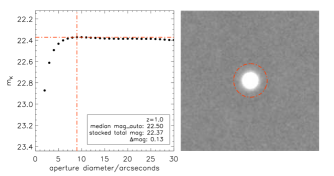
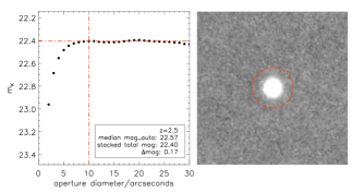
Figure 1: Examples of the stacking analysis used to determine the best correction between $2^{\prime\prime}-$diameter aperture fluxes and total fluxes at $z=1$ (left) and $z=2.5$ (right). In both cases the right-hand sub-panel shows the stacked image of galaxies within the mag_auto range $22<m_{\rm auto}<23$. The left-hand sub-panels show the corresponding curve-of-growth, where the horizontal red dashed line shows the best estimate of the total magnitude. The vertical red dashed line shows the aperture diameter that encloses the total flux, which can be seen as the red circular aperture in the right-hand sub-panels. The inset legends show the value of $\Delta$mag between the curve-of-growth estimate of total magnitude and the median mag_auto of those galaxies entering the stack.

2.5 Correction to total magnitude

The UltraVISTA photometry was initially measured in $2^{\prime\prime}-$diameter circular apertures before being corrected to total magnitudes based on the ratio of flux_auto to flux_aper in the $K_{s}$-band. This is a fairly standard approach to correcting to total magnitudes, and relies on the assumption that the Kron-like magnitudes (Kron 1980) measured by sextractor (i.e. mag_auto) capture $\simeq 90\%$ of the integrated galaxy light (depending on the form of the radial surface-brightness profile). However, the different techniques commonly adopted to correct to total magnitudes have been the subject of extensive discussion in the recent literature, with variations in the methods adopted for bright objects being blamed for inconsistencies between different determinations of the bright end of the galaxy luminosity function (e.g. Bernardi et al. 2013; D’Souza, Vegetti & Kauffmann 2015; Loveday et al. 2015).

In order to address this issue, we produced stacked $K_{s}$-band images of our final galaxy sample as a function of redshift and apparent $K_{s}$-band magnitude. To ensure that flux from nearby bright companions did not mimic extended wings to the stacked radial surface-brightness profiles, the stacking was confined to the 65$\%$ of the final $K_{s}$-band galaxies with no companions within a radius of $4^{\prime\prime}$ with fluxes greater than 50% of the flux of the primary object. Postage-stamp $K_{s}$-band images of each galaxy were generated, sky-subtracted and cleaned of nearby companion objects. Each postage-stamp image was initially sky-subtracted using the median of all sky pixels at radii $\geq 5^{\prime\prime}$ (as indicated by the sextractor segmentation map). Additionally, a further level of sky-subtraction was applied by fitting a two-dimensional surface (first order polynomial) to all sky pixels, excluding all pixels within a radius of 7.5^′′ from the central object.

After this cleaning process, median stacks of the objects in each redshift and apparent magnitude bin were produced. When constructing the median stacks, all pixels identified by sextractor as belonging to companion objects were excluded. A non-parametric measurement of the total flux in each stacked image was then derived using a curve-of-growth analysis. Example curve-of-growth plots can be seen in Fig. 1.

The results of the curve-of-growth analysis demonstrated that the total flux recovered from the stacked images was systematically larger than the median value of flux_auto for the objects included in the stack. Interestingly, the off-set between the total stacked flux and the median flux_auto of the stacked galaxies varied very little with either redshift or apparent $K_{s}$-band magnitude. The median offset was 13.5%, with the off-set always lying within the range $9-18\%$. Consequently, throughout the rest of this analysis we adopt 1.135$\times$flux_auto as our best estimate of the total flux for the UltraVISTA galaxies. Based on an identical stacking analysis of the $H_{160}$ imaging in the two CANDELS fields, no systematic off-set was found between the curve-of-growth fluxes and the total fluxes determined by Guo et al. (2013) and Galametz et al. (2013). As a consequence, no correction was applied to the CANDELS photometry.

As part of this analysis, a stack of several hundred isolated stars was used to accurately measure the correction between $2^{\prime\prime}-$diameter magnitudes and total magnitudes for point sources in the PSF homogenised UltraVISTA data. The resulting correction of $-0.43$ magnitudes was then used as a minimum correction for all galaxies, i.e. no object was assigned a correction smaller than this. The minimum correction was applied in order to ensure that no galaxies were corrected by an amount less than expected for an unresolved point source.

3 Sample selection

In this section we describe the process of constructing the final sample of $0.25~{}\leq~{}z~{}\leq~{}3.75$ galaxies, based on spectral energy distribution (SED) fitting of the photometry catalogues described above. The upper limit to the redshift interval was specifically chosen to provide three photometric data points sampling the galaxy SED long-ward of the $4000$Å  break (i.e. $K_{s}$, $3.6\mu$m & $4.5\mu$m), with the Spitzer IRAC photometry always providing a measurement of the rest-frame SED at $\lambda_{\rm rest}\geq 1\mu$m. This situation naturally limits the uncertainties involved in calculating the absolute $K$-band magnitude for each galaxy.

In addition to the SED fitting process, we also describe the simulations performed in order to calculate completeness corrections and how the galaxy sample was cleaned of galactic stars, artefacts and potential active galactic nuclei (AGN).

3.1 Star-galaxy separation

Before calculating photometric redshifts, the galaxy sample was first cleaned of galactic stars. Within the UltraVISTA dataset, this was initially performed by removing objects lying on the stellar locus in the ($Y-J$) vs ($H-K$) colour-colour diagram. As a secondary check, objects consistent with the stellar locus on the ($g^{\prime}-i^{\prime}$) vs ($J-K$) colour-colour diagram were also removed (see McCracken et al. 2012 and Jarvis et al. 2013 for examples of star-galaxy separation in data sets of this size). Due to their small area, the stellar loci in the CANDELS datasets are poorly defined. However, due to the high-spatial resolution of the HST imaging, star-galaxy separation is relatively straightforward. Consequently, we removed all point-like objects with sextractor parameter class_star$>$0.98, a threshold demonstrated to efficiently isolate objects with stellar colours by Galametz et al. (2013).

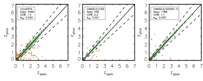
Figure 2: A comparison of spectroscopic and photometric redshifts within the final galaxy sample. The left-hand panel shows $z_{phot}$ vs $z_{spec}$ for UltraVISTA deep and wide combined, whereas the middle and right-hand panels show the equivalent information for the CANDELS/UDS and CANDELS/GOODS-S fields respectively. The black solid lines show the one-to-one relation and the black dashed lines show the cut used for identifying catastrophic outliers (i.e. $\left|dz\right|>0.15$). Catastrophic outliers are plotted in orange, while those objects with acceptable photometric redshifts are plotted in green. The inset panels list the basic statistics of the comparison in each field: number of spectroscopic objects ($N_{obj}$), percentage of catastrophic outliers (CO%) and $\sigma_{dz}$.

3.2 SED fitting

Following the removal of galactic stars, photometric redshifts were computed using template-based SED fitting to the PSF-matched photometry catalogues described in Section 2. The final photometric redshifts adopted for the analysis were the median of five different estimates produced using different codes and different template sets. The different photometric redshift code+template configurations were as follows:

1. Two sets of photometric redshifts were generated using the publicly available SED fitting code lephare (Arnouts et al. 1999; Ilbert et al. 2006), both assuming solar metallicity, the Calzetti et al. (2000) dust attenuation law with E(B-V) values in the range $0.0-0.5$ and including emission lines. The first photometric redshift run employed the zcosmos template set (Ilbert et al., 2009) while the second employed the pégase template set.

2. A further two sets of photometric redshifts were generated using the publicly available EAZY code (Brammer, van Dokkum & Coppi 2008) using the PCA (Blanton & Roweis 2007) and pégase template sets (Fioc & Rocca-Volmerange 1999).

3. The final set of photometric redshift results was generated using a private SED fitting code (McLure et al. 2011; McLeod, McLure & Dunlop 2016) employing Bruzual & Charlot (2003) (BC03) templates with metallicities in the range $0.2Z_{\odot}-Z_{\odot}$ and the addition of strong emission lines. This photometric redshift set-up employed the Calzetti et al. (2000) dust attenuation law, allowing $A_{V}$ to vary within the range $0.0\leq A_{V}\leq 2.5$.

A comparison between our final median photometric redshifts and publicly available spectroscopic redshifts is shown in Fig. 2. It can be seen that our photometric redshift results have a typical value of $\sigma_{dz}\simeq 0.02$ (calculated using the MAD estimator), where $dz=z_{spec}-z_{phot}/(1+z_{spec})$. Using the standard definition of catastrophic outliers as those objects with $\left|dz\right|>0.15$, the typical catastrophic outlier rate is $\simeq 1-2\%$. These results indicate that our photometric redshifts are robust and do not vary in quality between the space-based and ground-based photometry.

In order to calculate the final values of absolute $K$-band magnitude ($M_{K}$), the SED of each galaxy was fit for a final time (at fixed redshift) using a sub-set of BC03 templates defined by Wuyts et al. (2011). This set of templates consists of exponentially decaying star-formation histories with values of $\tau$ in the range $0.3\leq\tau\leq 10$ Gyr and ages in the range 50 Myr to the age of the Universe. Dust extinction was applied using the Calzetti et al. (2000) attenuation law with E(B$-$V) allowed to vary within the range $0.0-0.5$ and metallicity was fixed at solar.

The advantage of this template sub-set is that it produces star-formation rate (SFR) estimates which are in good agreement with estimates of total SFRs calculated from the addition of raw UV star formation and dust obscured star formation measured at sub-mm wavelengths (Wuyts et al., 2011). However, it should be noted that, given a fixed redshift and multi-wavelength data covering the observed wavelength range $0.38\mu$m $\leq\lambda\leq 4.5\mu$m, the derived values of absolute $K$-band magnitude are not very dependent on the assumed SED template set. The distribution of absolute $K$-band magnitude versus redshift for the final sample is shown in Fig. 3, where the values of $M_{K}$ have been corrected to total according to the prescription described in Section 2.5.

3.3 Completeness

When measuring the KLF it is vital to accurately calculate the completeness limits of the data, particularly when trying to measure the faint-end slope. In order to compute the completeness, a synthetic galaxy population was created in each field, covering the redshift range $0.25\leq z\leq 3.75$ and the appropriate range in $M_{K}$ for that dataset. The number densities as a function of magnitude were based on the Cirasuolo et al. (2010) parameterisation of the evolving KLF although, given our final choice of conservative cuts (see below), the exact input KLF parameters do not have a significant impact on the final completeness corrections.

Each member of the synthetic galaxy population was randomly allocated an SED template taken from the catalogue of SED fits to members of the real galaxy sample, matched within $\Delta z=\pm 0.25$ and $\Delta M_{K}=\pm 0.25$ magnitudes. Based on the adopted SED template, the synthetic galaxy was injected as a point source into the relevant UltraVISTA or CANDELS imaging data with the appropriate $K$-band or $H_{160}$-band apparent magnitude. The completeness as a function of apparent magnitude and redshift was then calculated by analysing the images containing the synthetic sources with an identical sextractor configuration to that employed when selecting the original samples. See Fig. 3 for the completeness of each survey as a function of redshift.

3.4 Final cleaning

Before proceeding to measure the KLF, the galaxy sample was cleaned of objects with erroneous photometry and potential AGN. The first stage in this process was to remove the 5% of objects with the poorest quality SED fits as indicated by their $\chi^{2}$ values. Given the anti-correlation between redshift and $\chi^{2}$, this cleaning was done separately within the six redshift bins adopted for the rest of the analysis. The vast majority of objects excluded on the basis of their high $\chi^{2}$ were either artefacts or objects whose photometry was contaminated/corrupted in one or more filters.

The second stage in the final cleaning process was to exclude potential AGN. Within the UltraVISTA dataset, all sources were removed which were detected in either the Chandra Cosmos survey (C-COSMOS; Elvis et al. 2009) or the VLA-COSMOS Large Project (Schinnerer et al. 2007). Finally, we also used the S-COSMOS 24$\mu$m catalogue (Sanders et al., 2007) to remove potential obscured AGN. This was achieved by converting the 24$\mu$m flux into a measurement of specific SFR (SSFR) using the Rieke et al. (2009) IR templates and stellar masses computed using the same SED templates as in Section 3.2. The 24$\mu$m SSFR distribution shows a clear bi-modality with the high SSFR peak being defined as log${}_{10}(SSFR/\rm Gyr^{-1})>0.75$. The peak is dominated by $z>2$ objects where the 24$\mu$m is sampling hot dust which is likely AGN heated. We therefore remove all objects within UltraVISTA in the high peak of this distribution in the redshift range $0.25\leq z\leq 3.75$. The combination of both AGN cleaning methods resulted in removal of 7% of the sample across the full redshift range. Within the CANDELS/UDS dataset we excluded potential AGN on the basis of the X-ray/radio detections provided in the publicly available photometry catalogue (Galametz et al., 2013). For the CANDELS/GOODS-S dataset, potential AGN were excluded by matching to the X-ray, radio and IR-selected AGN candidates compiled by Kocevski et al. (2012).

After completing the final cleaning process it was possible to construct the final galaxy sample to be used in the computation of the KLF. Fortunately, the different datasets used to construct the final galaxy sample cover ranges in $K$-band luminosity which overlap significantly. As a result, it was possible to adopt a conservative approach and only include a galaxy in the final sample if it survived the full cleaning process and was brighter than the 95% completeness limit for its redshift within the survey from which it was originally selected. The distribution of the final galaxy sample on the $M_{K}-z$ plane is shown in Fig. 3, along with the 95% completeness limits for the various different surveys.

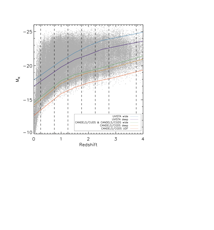
Figure 3: Redshift versus absolute $K$-band magnitude for the final galaxy sample (grey data points). The black vertical dashed lines show the limits of the redshift bins employed in the rest of the analysis, and the coloured solid lines are the 95% completeness limits of the five different surveys used in this work.

4 Luminosity function fitting

Armed with the final galaxy sample, the KLF was derived using the classical $\frac{1}{V_{max}}$ (Schmidt 1968) maximum likelihood estimator, defined as follows:

$$\phi(M_{K})\Delta M=\sum\limits_{i=1}^{N_{gal}}\frac{1}{C(M_{K},z)V_{max,i}}$$ (1)

where $\phi(M_{K})$ is the number density in a given absolute $K$-band magnitude bin, $V_{max,i}$ is the maximum volume a given object can be associated with and still be included within the sample, $C(M_{K},z)$ is the completeness as a function of absolute $K$-band magnitude and redshift (as computed in Section 3.3) and $\Delta M$ is the bin size in magnitudes.

The full uncertainties associated with the number densities are a combination of Poisson error ($\sigma_{poi}$), error due to template fitting ($\sigma_{temp}$), and cosmic variance ($\sigma_{cv}$). The Poisson contribution is computed as:

$$\sigma_{poi}=\sum\limits_{i=1}^{N_{gal}}\sqrt{\frac{1}{C(M_{K},z)V_{max,i}}}$$ (2)

The template fitting error ($\sigma_{temp}$) is computed from Monte Carlo simulations which account for the uncertainties introduced from the errors in object photometry and potential mismatches between the real galaxy SEDs and the adopted model templates. In this process, 100 realisations of the KLF across all redshift bins were computed, with each individual galaxy randomly allocated a redshift, drawn from its P(z) distribution, and allocated updated values of $M_{K}$ and completeness. The value of $\sigma_{temp}$ in a given redshift and $M_{K}$ bin was then calculated from the distribution of number densities returned by the Monte Carlo realisations. As described previously, the final adopted redshift for each galaxy was the median of five separate photometric redshift runs, each of which delivered a $1\sigma$ upper and lower confidence region (i.e. $z_{min}<z_{phot}<z_{max}$). Consequently, the P(z) for each object was modelled as a two-sided Gaussian function, centred on the median redshift ($z_{med}$) with the upper and lower sigma values set to $\sigma_{high}=z_{max}-z_{med}$ and $\sigma_{low}=z_{med}-z_{min}$ respectively. In order to be conservative, the values of $z_{max}$ and $z_{min}$ adopted to construct the P(z) distributions were the extreme values returned by the five photometric redshift runs.

Finally, we compute the value of $\sigma_{cv}$ at a given redshift and within a given $M_{K}$ bin. Given that our final dataset is effectively the combination of five different surveys, we are able to use the variation in galaxy number density within a given $M_{K}$ and redshift bin as an empirical measurement of the cosmic variance uncertainties. The final uncertainty on the number density calculated at a given redshift and within a given $M_{K}$ bin was then taken as:

$$\sigma_{\phi(M_{K})}=\sqrt{(\sigma_{poi}^{2}+\sigma_{temp}^{2}+\sigma_{cv}^{2})}$$ (3)

In our faintest magnitude bins, where we only have data from the UDF, we cannot estimate the cosmic variance uncertainty using our standard method, and make the assumption that Poisson and template uncertainties are dominant. To test this assumption we estimated the cosmic variance in these bins according to the prescription of Moster et al. (2011). This calculation suggests that the total error in the faintest bins would likely be increased by only $\sim 20$%, confirming that the Poisson and template uncertainties are dominant. Fitting the KLF data with and without this additional contribution results in best-fitting parameters and uncertainties which are virtually identical to those presented in Table 4.

4.1 Schechter-function fits

Throughout the analysis we employ $\chi^{2}$ fitting to the binned KLF data using either single or double Schechter functions. The single Schechter function has the following form:

$$\phi(M)=0.92\phi^{*}\cdot(10^{-0.4(M-M^{*})})^{(1+\alpha)}e^{[-10^{-0.4(M-M^{*})}]}$$ (4)

where $\phi^{*}$ is the normalisation, M^∗ is the characteristic magnitude and $\alpha$ is the faint-end slope. The double Schechter function is parameterised as follows:

$$\phi(M)=0.92\cdot 10^{-0.4(M-M^{*})}e^{[-10^{-0.4(M-M^{*})}]}\\ \cdot[\phi_{1}^{*}\cdot 10^{-0.4(M-M^{*})\alpha_{1}}+\phi_{2}^{*}\cdot 10^{-0.4(M-M^{*})\alpha_{2}}]$$ (5)

where M^∗ is the shared characteristic magnitude and ($\phi_{1},\alpha_{1}$) and ($\phi_{2},\alpha_{2}$) are the normalisations and faint-end slopes of the two Schechter-function components.

4.2 The local $K$-band luminosity function

Before proceeding to explore the evolution of the KLF, it is clearly desirable to have a robust measurement of the local KLF to serve as a baseline. In Fig. 4 we show the local KLF based on data from the UKIDSS LAS (Smith, Loveday & Cross 2009) and GAMA surveys (Driver et al. 2012). The KLF data from Smith, Loveday & Cross (2009) was converted to total magnitudes assuming $K_{AB}=K_{vega}+1.9$ and $K_{\rm tot}-K_{\rm Petrosian}=-0.2$, whereas the KLF data from Driver et al. (2012) was converted to total magnitudes assuming $K_{\rm tot}-K_{\rm Kron}=-0.1$.

After making the necessary corrections, it can be seen from Fig. 4 that the Smith, Loveday & Cross (2009) and Driver et al. (2012) datasets are completely compatible and, as a result, a combined fit to both datasets was performed in order to derive our fiducial local KLF parameters. In Fig. 4 the best-fitting single and double Schechter-function fits are shown as the solid black and dashed yellow lines respectively. The dashed purple line shows the best-fitting double Schechter function with faint-end slopes fixed at $\alpha_{1}=-0.5$ and $\alpha_{2}=-1.5$ (see Section 6 for a discussion). The best-fitting parameters corresponding to the three fits shown in Fig. 4 are listed in Table 2

As might be expected, our single Schechter-function fit to the combined local KLF data is intermediate to those derived by Smith, Loveday & Cross (2009) and Driver et al. (2012), and is in good agreement with previous fits reported by Kochanek et al. (2001) and Cole et al. (2001). It can be seen from Fig. 4 that the local KLF is reasonably well matched by a single Schechter function at magnitudes brighter than $M_{K}\simeq-20$, with convincing evidence for an up-turn in the number density of galaxies only apparent within the faintest few magnitude bins. Formally the best-fitting double Schechter function has a very steep faint-end slope ($\alpha_{2}=-2.35\pm 0.30$), although the lack of dynamic range in luminosity means that the slope and normalisation of this component are not very well constrained. The uncertainty in the slope of the second Schechter function component can clearly be seen in Fig. 4, where the best-fitting double Schechter function (yellow dashed line) is virtually indistinguishable from the double Schechter-function fit with the faint-end slope fixed at $\alpha_{2}=-1.5$ (purple dashed line).

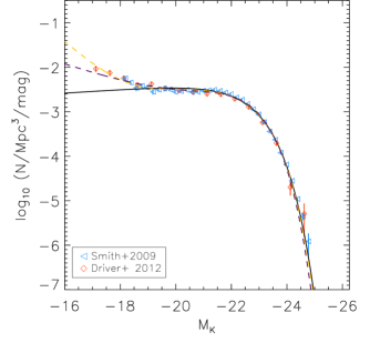
Figure 4: The local $K$-band galaxy luminosity function as measured by Smith, Loveday & Cross (2009) and Driver et al. (2012). The solid black and dashed yellow lines are our best-fitting single and double Schechter-function fits to the combined dataset respectively. The dashed purple line shows our best-fitting double Schechter function with fixed faint-end slopes of $\alpha_{1}=-0.5$ and $\alpha_{2}=-1.5$ (see Section 6 for a discussion).

Table 2: The best-fitting single and double Schechter-function parameters for the local KLF dataset shown in Fig. 4. Columns $2-6$ list the best-fitting parameters and their corresponding uncertainties. Columns 7 & 8 list the corresponding values of $\chi^{2}$ and reduced $\chi^{2}_{\nu}$ respectively. The final row shows the results of fitting the local KLF dataset with the constrained double Schechter function discussed in Section 6. Given the small statistical errors associated with the local KLF dataset shown in Fig. 4, none of the Schechter-function fits are formally acceptable. As a result, the parameter uncertainties quoted in the table have been calculated after inflating the errors to enforce $\chi^{2}_{\nu}=1$.

Schechter fit	$\log(\phi_{1}^{*}/\rm{Mpc}^{-3})$	$M_{K}^{*}$	$\alpha_{1}$	$\log(\phi_{2}^{*}/\rm{Mpc}^{-3})$	$\alpha_{2}$	$\chi^{2}$	$\chi^{2}_{\nu}$
single	$-$2.29 $\pm$0.02	$-$22.35 $\pm$ 0.02	$-$0.90 $\pm$ 0.02			183.6	3.9
double	$-$2.26 $\pm$0.02	$-$22.29 $\pm$ 0.03	$-$0.80 $\pm$ 0.04	$-$4.79 $\pm$ 0.53	$-$2.35 $\pm$ 0.30	102.9	2.3
double	$-$2.28 $\pm$0.02	$-$22.16 $\pm$ 0.02	$-$0.50 (fixed)	$-$3.13 $\pm$ 0.03	$-$1.50 (fixed)	161.2	3.4

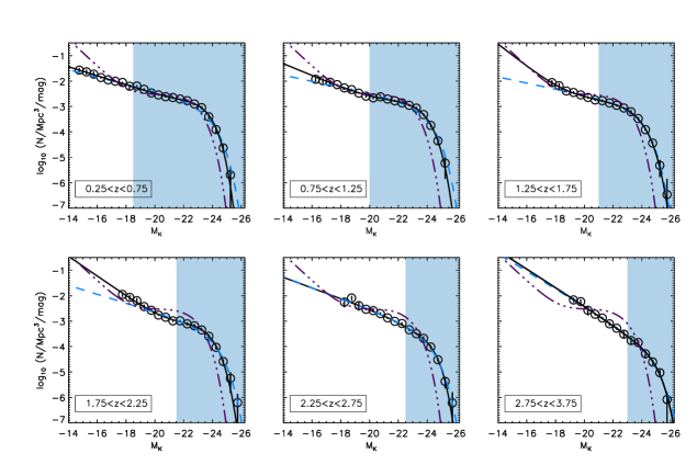
Figure 5: The evolving KLF dataset together with the best-fitting single and double Schechter functions. In each redshift bin the black solid circles are the number densities of the combined UltraVISTA+CANDELS+HUDF dataset, and the solid black and dashed blue lines are the best-fitting double and single Schechter functions respectively. For reference, in each panel we also show our best-fitting double Schechter-function fit to the local KLF dataset as the dot-dashed purple line. The blue shaded areas highlight the luminosity range where the data are dominated by the ground based UltraVISTA imaging.

Table 3: The binned ($1/V_{\rm max}$) measurements of the KLF within the six redshift bins shown in Fig. 5. Column one lists the absolute $K$-band luminosity bins and columns $2-7$ list the individual values of $\phi_{k}$ and their corresponding uncertainties. The values of $\phi_{k}$ and their uncertainties are quoted in units of $10^{-4}$mag^-1Mpc^-3.

	$0.25\leq z\leq 0.75$	$0.75\leq z\leq 1.25$	$1.25\leq z\leq 1.75$	$1.75\leq z\leq 2.25$	$2.25\leq z\leq 2.75$	$2.75\leq z\leq 3.75$
$M_{K}$	$\phi_{k}$	$\phi_{k}$	$\phi_{k}$	$\phi_{k}$	$\phi_{k}$	$\phi_{k}$
$-$14.75	269.8 $\pm$ 56.8
$-$15.25	231.6 $\pm$ 52.4
$-$15.75	187.0 $\pm$ 46.3
$-$16.25	137.7 $\pm$ 13.6	118.0 $\pm$ 27.2
$-$16.75	112.3 $\pm$ 08.4	103.7 $\pm$ 23.9
$-$17.25	098.9 $\pm$ 08.6	090.5 $\pm$ 23.8
$-$17.75	088.5 $\pm$ 06.7	072.3 $\pm$ 04.4	087.4 $\pm$ 019.3	112.4 $\pm$ 022.8
$-$18.25	062.8 $\pm$ 10.9	053.8 $\pm$ 03.9	065.6 $\pm$ 017.8	086.3 $\pm$ 018.7	056.0 $\pm$ 021.0
$-$18.75	063.9 $\pm$ 05.3	046.2 $\pm$ 04.4	040.9 $\pm$ 005.0	063.8 $\pm$ 016.6	081.9 $\pm$ 017.6
$-$19.25	047.5 $\pm$ 04.7	033.6 $\pm$ 02.1	035.6 $\pm$ 004.3	037.6 $\pm$ 007.3	040.9 $\pm$ 015.0	068.4 $\pm$ 014.8
$-$19.75	034.2 $\pm$ 02.2	025.6 $\pm$ 03.1	028.6 $\pm$ 002.8	026.8 $\pm$ 001.7	029.4 $\pm$ 002.9	058.7 $\pm$ 013.3
$-$20.25	028.6 $\pm$ 02.1	021.9 $\pm$ 02.3	022.8 $\pm$ 002.5	017.3 $\pm$ 001.2	026.0 $\pm$ 003.7	026.8 $\pm$ 009.9
$-$20.75	024.4 $\pm$ 01.7	024.1 $\pm$ 02.2	018.1 $\pm$ 001.6	014.3 $\pm$ 001.2	019.7 $\pm$ 002.8	018.7 $\pm$ 002.3
$-$21.25	022.6 $\pm$ 02.7	019.7 $\pm$ 01.6	017.0 $\pm$ 001.8	010.3 $\pm$ 001.0	013.5 $\pm$ 001.1	013.3 $\pm$ 001.5
$-$21.75	019.7 $\pm$ 01.3	016.8 $\pm$ 01.4	013.8 $\pm$ 001.1	010.3 $\pm$ 000.8	009.9 $\pm$ 000.9	007.8 $\pm$ 001.3
$-$22.25	017.0 $\pm$ 01.9	013.9 $\pm$ 01.2	011.2 $\pm$ 001.2	007.8 $\pm$ 001.2	008.1 $\pm$ 001.1	005.3 $\pm$ 000.8
$-$22.75	012.6 $\pm$ 01.2	011.2 $\pm$ 01.0	008.8 $\pm$ 000.6	006.6 $\pm$ 001.2	004.6 $\pm$ 000.5	003.1 $\pm$ 000.9
$-$23.25	009.0 $\pm$ 01.4	008.7 $\pm$ 01.0	006.2 $\pm$ 001.1	004.5 $\pm$ 000.4	003.2 $\pm$ 000.3	001.7 $\pm$ 000.5
$-$23.75	003.9 $\pm$ 00.8	004.8 $\pm$ 00.5	003.4 $\pm$ 000.5	002.6 $\pm$ 000.5	002.1 $\pm$ 000.4	001.4 $\pm$ 000.3
$-$24.25	001.2 $\pm$ 00.4	001.8 $\pm$ 00.3	001.2 $\pm$ 000.1	00.93 $\pm$ 000.2	00.96 $\pm$ 000.2	000.5 $\pm$ 000.1
$-$24.75	00.24 $\pm$ 0.07	00.45 $\pm$ 0.13	00.36 $\pm$ 00.07	00.26 $\pm$ 00.06	00.30 $\pm$ 00.05	00.25 $\pm$ 00.06
$-$25.25	00.02 $\pm$ 0.02	00.06 $\pm$ 0.05	0.048 $\pm$ 0.031	0.056 $\pm$ 0.041	0.043 $\pm$ 0.020	0.094 $\pm$ 0.027
$-$25.75			0.003 $\pm$ 0.010	0.006 $\pm$ 0.074	0.006 $\pm$ 0.010	0.008 $\pm$ 0.008

5 The evolving $\mn@boldsymbol{K-}$band luminosity function

Our new determination of the evolving KLF over the redshift interval $0.25\leq z\leq 3.75$ is provided in Table 3 and plotted in Fig. 5. In each panel of Fig. 5 the best-fitting single Schechter function is shown as the dashed blue line and the best-fitting double Schechter function is shown as the solid black line. For reference, in each panel we also show our best-fitting double Schechter function to the local KLF as the dot-dashed purple line.

The light blue shaded region in each panel of Fig. 5 indicates the absolute magnitude range over which the final galaxy sample is dominated by the ground-based data from UltraVISTA, with the deep HST imaging from CANDELS and the HUDF dominating at fainter magnitudes.

Table 4: The best-fitting single and double Schechter parameters based on fitting the KLF data shown in Fig. 5 and Table 3. The first column lists the redshift bin and columns $2-6$ list the best-fitting Schechter function parameters and their corresponding uncertainties. Columns seven and eight list the corresponding values of $\chi^{2}$ and reduced $\chi^{2}_{\nu}$ respectively.

Redshift Range	$\log(\phi_{1}^{*}/\rm{Mpc}^{-3})$	$M_{K}^{*}$	$\alpha_{1}$	$\log(\phi_{2}^{*}/\rm{Mpc}^{-3})$	$\alpha_{2}$	$\chi^{2}$	$\chi^{2}_{\nu}$
0.25$<z<$0.75	$-$2.89 $\pm$ 0.06	$-$23.50 $\pm$ 0.12	$-$1.36 $\pm$ 0.02			45.3	2.5
0.75$<z<$1.25	$-$2.92 $\pm$ 0.07	$-$23.71 $\pm$ 0.13	$-$1.31 $\pm$ 0.03			44.8	3.0
1.25$<z<$1.75	$-$2.95 $\pm$ 0.05	$-$23.56 $\pm$ 0.07	$-$1.30 $\pm$ 0.03			12.1	0.9
1.75$<z<$2.25	$-$3.28 $\pm$ 0.12	$-$23.83 $\pm$ 0.18	$-$1.44 $\pm$ 0.07			39.1	3.0
2.25$<z<$2.75	$-$3.36 $\pm$ 0.06	$-$23.89 $\pm$ 0.10	$-$1.54 $\pm$ 0.04			07.7	0.6
2.75$<z<$3.75	$-$3.96 $\pm$ 0.16	$-$24.50 $\pm$ 0.20	$-$1.87 $\pm$ 0.15			04.8	0.5
0.25$<z<$0.75	$-$2.59 $\pm$ 0.06	$-$22.77 $\pm$ 0.16	$-$0.28 $\pm$ 0.29	$-$2.95 $\pm$ 0.10	$-$1.44 $\pm$ 0.04	11.7	0.7
0.75$<z<$1.25	$-$2.65 $\pm$ 0.06	$-$23.16 $\pm$ 0.15	$-$0.72 $\pm$ 0.23	$-$3.44 $\pm$ 0.29	$-$1.59 $\pm$ 0.11	08.4	0.7
1.25$<z<$1.75	$-$2.82 $\pm$ 0.07	$-$23.36 $\pm$ 0.13	$-$1.11 $\pm$ 0.16	$-$4.67 $\pm$ 1.38	$-$2.11 $\pm$ 0.58	02.9	0.3
1.75$<z<$2.25	$-$2.88 $\pm$ 0.07	$-$23.17 $\pm$ 0.16	$-$0.77 $\pm$ 0.23	$-$3.97 $\pm$ 0.33	$-$1.97 $\pm$ 0.15	06.7	0.6
2.25$<z<$2.75	$-$3.49 $\pm$ 0.18	$-$23.18 $\pm$ 0.30	$-$0.26 $\pm$ 0.69	$-$3.17 $\pm$ 0.15	$-$1.53 $\pm$ 0.08	05.7	0.6
2.75$<z<$3.75	$-$3.91 $\pm$ 0.36	$-$23.92 $\pm$ 0.66	$-$0.59 $\pm$ 1.46	$-$3.81 $\pm$ 0.45	$-$1.91 $\pm$ 0.15	03.7	0.5

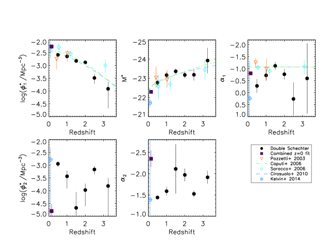
Figure 6: The redshift evolution of the parameters describing the double Schechter function fits to the KLF dataset. The top three panels show the evolution of the parameters of the Schechter component which describes the bright end of the KLF. The two bottom panels show the evolution of the Schechter component which describes the up-turn in galaxy number density seen at faint magnitudes. In addition to the results for the six redshift bins shown in Fig. 5, we also plot the parameters derived from the local KLF study of Kelvin et al. (2014) and our own double Schechter-function fit to the combined local KLF dataset shown in Fig. 4. The green and blue lines plotted in the upper panels are the fits to the evolving (single Schechter) parameters derived by Caputi et al. (2006) and Cirasuolo et al. (2010) respectively (both studies fixed the faint-end slope at $\alpha=-1.07$).

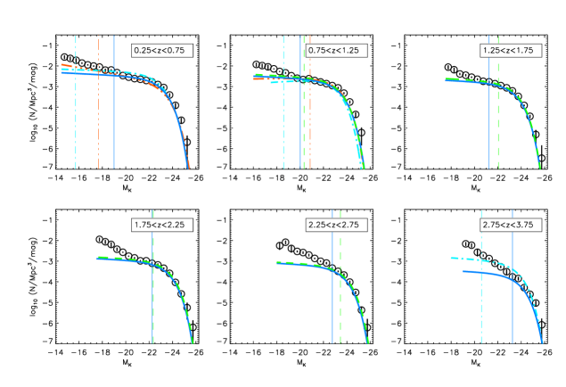
Figure 7: A comparison between our new measurement of the evolving KLF and the Schechter function fits derived by previous observational studies. The red triple-dot-dashed lines show the Schechter-function fits from Pozzetti et al. (2003), the light blue dot-dashed lines are the fits from Saracco et al. (2006), the green dashed lines are the fits from Caputi et al. (2006) and the blue solid lines are the fits from Cirasuolo et al. (2010). The corresponding vertical lines are the magnitude limits of the previous studies.

5.1 Single versus Double Schechter fits

Although it is now established that the local KLF cannot be well reproduced by a single Schechter function (e.g. Smith, Loveday & Cross 2009; Kelvin et al. 2014), previous studies of the evolving KLF have not possessed the combination of wide area and depth necessary to accurately determine its functional form at $z\geq 1$ (e.g. Caputi et al. 2006; Cirasuolo et al. 2010). The galaxy sample assembled for this study allows us to test the functional form of the evolving KLF at $z\geq 1$ for the first time.

The best-fitting parameters and the corresponding minimum $\chi^{2}$ values for the Schechter-function fits shown in Fig. 5 are provided in Table 4. As expected, the double Schechter function provides a better fit to the KLF data in all six redshift bins. However, it is not the case that the double Schechter fit can be statistically preferred to the single Schechter fit in all cases. Fortunately, given that the single Schechter-function fits form a nested sub-set of the double Schechter-function fits, it is straightforward to decide whether the double fit is statistically preferred. In this scenario, we expect the $\Delta\chi^{2}$ between the best-fitting models (i.e. $\Delta\chi^{2}=\chi^{2}_{\rm{single}}-\chi^{2}_{\rm{double}}$) to follow a $\chi^{2}$ distribution with two degrees of freedom, since the double Schechter has two more free parameters than the single Schechter function. Consequently, if the double fit is to be preferred over the single fit at the $99\%$ confidence level, we require a value of $\Delta\chi^{2}\geq 9.2$ between the two competing model fits.

It can be seen from the information presented in Table 4 that the double Schechter-function fit is formally preferred to the single Schechter-function fit at $\geq 99\%$ confidence within the first four redshift bins. Within the final two redshift bins the double Schechter function is not statistically preferred over the single fit. This conclusion agrees well with a visual inspection of Fig. 5, which also indicates that the extra freedom provided by the double Schechter function is not actually required to describe the data in the two highest redshift bins.

Overall it is clear that our new UltraVISTA+CANDELS+HUDF dataset indicates that the KLF has a double Schechter form out to redshifts of $z\simeq 2$, but that a double Schechter function is not formally required to describe the KLF data at $2.25\leq z\leq 3.75$. However, it is not immediately clear whether the apparent change in functional form at $z\simeq 2$ indicates a genuine transition or, alternatively, it simply reflects a combination of smoothing of the intrinsic KLF features due to photometric redshift uncertainties and the inevitable bias towards deriving steep faint-end slopes when dealing with a reduction in the available dynamic range in luminosity (c.f. Parsa et al. 2016). This issue is discussed further in Section 6.

5.2 Evolving Schechter function parameters

The redshift evolution of the best-fitting double Schechter-function parameters is shown in Fig. 6. The panels in the top row show the evolution of the three parameters which describe the Schechter component that dominates the bright end of the KLF, whereas the bottom panels show the evolution of the normalisation and slope of the component that dominates the faint end of the KLF.

The top-left panel shows a steady decrease in the value of $\log(\phi_{1}^{\star}/{\rm Mpc^{-3}})$, from a local value of $\simeq-2.3$ to a value of $\simeq-4.0$ by $z\simeq 3.5$. Likewise, it can be seen that $M_{K}^{\star}$ also shows a relatively smooth evolution with redshift, changing from $\simeq-22.3$ locally to $\simeq-23.8$ by $z\simeq 3.5$. In contrast, the value of $\alpha_{1}$ shows no real evolutionary trend, with a mean (median) value of $\langle\alpha_{1}\rangle=-0.54\pm 0.18(-0.66)$. Likewise, the bottom panels of Fig. 6 suggests that neither $\alpha_{2}$ or $\phi_{2}^{\star}$ show any convincing trend with redshift, with mean (median) values of $\langle\alpha_{2}\rangle=-1.76\pm 0.10(-1.75)$ and $\langle\log(\phi_{2}^{\star}/{\rm Mpc^{-3}}\rangle=-3.67\pm 0.23(-3.63)$ respectively.

To first order, the parameters shown in the top row are expected to mimic those that would be obtained by fitting a single Schechter function to only the bright end of our KLF data set (i.e. $M_{K}\leq-21$). To illustrate this point, in the top row of Fig. 6 we plot the parameter values derived by four previous studies of the evolving KLF, based on fitting single Schechter functions to data with a lower dynamic range in $K$-band luminosity. Within the errors, it can be seen that the parameters derived by previous literature studies, using single Schechter-function fits to only the bright end of the evolving KLF, agree with the ($M_{K}^{\star},\phi_{1}^{\star}$) parameters derived here by fitting a double Schechter function over a much greater dynamic range in $K$-band luminosity.

In summary, the results plotted in Fig. 6 suggest that it may be possible to describe the evolution of the KLF using a double Schechter function, in which the bright-end component evolves smoothly with redshift while the faint-end component remains approximately constant. This prospect is pursued further in Section 6.

5.3 Comparison to previous observational results

To explore the agreement with previous literature results further, in Fig. 7 we compare our new KLF dataset with the best-fitting single Schechter functions derived by Pozzetti et al. (2003), Caputi et al. (2006), Saracco et al. (2006) and Cirasuolo et al. (2010).

As can readily be seen from Fig. 7, the single Schechter-function fits derived by the four previous literature studies continue to provide a good description of our new KLF dataset, at least down to the magnitude limits explored by the previous studies. In the first two redshift bins there is some evidence that our bright-end data-points are somewhat brighter than the literature Schechter-function fits. However, this is expected given our revised treatment for correcting to total magnitudes which accounts for extended light at large radii.

The comparison shown in Fig. 7 clearly demonstrates that the relatively flat faint-end slopes (i.e. $\alpha\simeq-1$) derived (or assumed) by previous studies completely fail to describe the up-turn in the number density of galaxies at fainter magnitudes revealed by our new UltraVISTA+CANDELS+HUDF dataset. This graphically re-enforces the conclusion that a double Schechter function is necessary to simultaneously match the steep decrease in number density at $M_{K}<M_{K}^{\star}$ and the up-turn seen at fainter magnitudes.

5.4 Comparison to simulation results

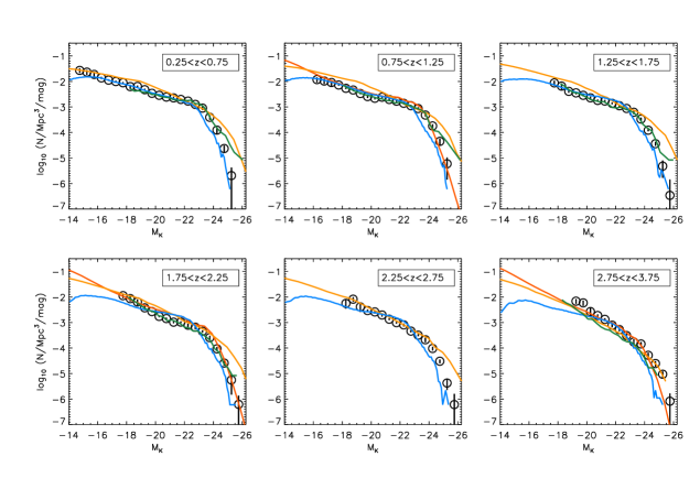
Figure 8: A comparison between our new measurement of the evolving KLF and the predictions of four recent galaxy-evolution models. The yellow line shows the predictions of the Illustris hydro-dynamical simulation (Genel et al., 2014), the dark green line shows the predictions of the mufasa hydro-dynamical simulation (Davé, Thompson & Hopkins, 2016), the red line shows the predictions of the Henriques et al. (2015) semi-analytic model and the blue line shows the predictions of the Gonzalez-Perez et al. (2014) semi-analytic model. Predictions from the Henriques et al. (2015) and Davé, Thompson & Hopkins (2016) models are not presented in all redshift bins.

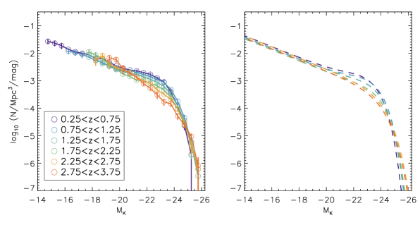
Figure 9: The left-hand panel shows an overlay of the KLF data from all six redshift bins. It can be seen immediately that the KLF data is consistent with having the same faint-end slope at $M_{K}\geq-20$. Moreover, it is clear that there appears to be very little evolution in the number density of galaxies brighter than $M_{K}\simeq-24.5$. Consequently, over the redshift interval $0.25\leq z\leq 0.75$ it appears that the evolution of the KLF consists largely of a relatively smooth build-up in the number density of intermediate luminosity galaxies, with absolute magnitudes in the range $-20\leq M_{K}\leq-24$. The right-hand panel shows the reproduction of the observed KLF evolution based on our simplified, 3-parameter prescription (see Section 6 for a discussion).

In Fig. 8 we compare our new KLF dataset to the predictions of four recent galaxy evolution simulations, two of which are semi-analytic in nature and two of which are hydro-dynamical. The first hydro-dynamical model is Illustris (yellow line; Genel et al. 2014), which is an N-body/hydro-dynamical simulation in which the physics governing galaxy formation and evolution is tuned to match the local galaxy stellar mass function (GSMF) and the evolution of the cosmic star-formation rate density. The second hydro-dynamical model is the recent mufasa simulation (dark green line; Davé, Thompson & Hopkins 2016), which employs an empirical prescription for quenching based on halo mass.

The red line in Fig. 8 shows the predictions of the Henriques et al. (2015) semi-analytic galaxy evolution model. This simulation is based on the Munich galaxy formation models, but includes updates which match observations of the passive fraction of galaxies in the redshift range $0<z<3$, as well as the evolution of the GSMF. Finally, the blue line in Fig. 8 shows the predictions of the Gonzalez-Perez et al. (2014) semi-analytic model, which is a recent update of galform (Cole et al. 2000). Importantly, the absolute $K$-band magnitudes predicted by all four models shown in Fig. 8 are based on Bruzual & Charlot stellar population models, and should therefore be directly comparable to our KLF dataset.

In the first three redshifts bins shown in Fig. 8, the predictions from the Gonzalez-Perez et al. (2014) model do a good job of reproducing the observed normalisation and faint-end slope of the KLF. However, at these redshifts there is a clear tendency to under-predict the number density of bright galaxies ($M_{K}\leq-23$), which appears to be the result of predicting a value of $M_{K}^{\star}$ that is $\simeq 0.5-1$ mag fainter than observed. In the three higher redshift bins the difference between predicted and observed $M_{K}^{\star}$ continues and the KLF predicted by the Gonzalez-Perez et al. (2014) model also displays a faint-end slope that is somewhat shallower than is observed.

The predictions of the Henriques et al. (2015) semi-analytic model do a good job of reproducing the normalisation and faint-end slope of the observed KLF over the redshift range $0.75\leq z\leq 3.75$. In particular, it is noticeable that the Henriques et al. (2015) model is able to accurately reproduce the bright end of the observed KLF at $z\simeq 1$ and $z\simeq 2$. In the highest redshift bin at $z\simeq 3.25$, the Henriques et al. (2015) model produces the best overall match to the observed data, although it does under-predict the number density of the very brightest galaxies.

The mufasa simulation does an excellent job of matching the normalisation, faint-end slope and break in the observed KLF at $z\leq 2.25$, displaying only a slight tendency to over-produce the very brightest galaxies at $z\leq 1.75$. Interestingly, it appears that the mufasa model can reproduce the inflection point observed in the KLF between the bright end and the up-turn seen at fainter magnitudes. In the highest redshift bin at $z\simeq 3.25$ the mufasa model mimics the shape of the observed KLF very well, but under-predicts the observed number densities by a constant factor of $\simeq 2$.

Finally, the Illustris model does a good job of matching the observed number densities around $M_{K}^{\star}$ at all redshifts, but consistently over-predicts the observed number densities at fainter and brighter magnitudes. Although the Illustris predictions shown in Fig. 8 do not include dust reddening, the tendency to over-predict the number density of galaxies at the extreme ends of the KLF is entirely consistent with comparisons between the Illustris simulation and observations of the evolving GSMF (Genel et al. 2014).

Overall, the comparison between the latest model predictions and our new determination of the evolving KLF are encouraging, with the Henriques et al. (2015) semi-analytic and mufasa (Davé, Thompson & Hopkins 2016) hydro-dynamical simulations doing a particularly good job of reproducing the observed data. In particular, although substantial differences remain in detail, particularly at the bright end, all of the models agree reasonably well on the basic shape/slope of the KLF at magnitudes fainter than the break.

The last detailed comparison between observations of the evolving KLF and simulation predictions was performed by Cirasuolo et al. (2010). At that time, simulation results appeared to significantly over-predict the number density of faint galaxies, although the limited dynamic range of the data available to Cirasuolo et al. (2010) only allowed the comparison to be made at magnitudes brighter than $M_{K}\simeq-20,M_{K}\simeq-22$ and $M_{K}\simeq-23$ at $z=1,2,\&\,3$ respectively.

The improvements in the quality of observational data over the last five years mean that it is now possible to perform this comparison to much fainter magnitudes over the full redshift range. Although the simulation results presented in Fig. 8 have typically been tuned to reproduce the stellar mass function (and therefore the KLF) at low redshift, it is encouraging that they continue to agree reasonably well, at least qualitatively, with the observed KLF over a broad range in redshift.

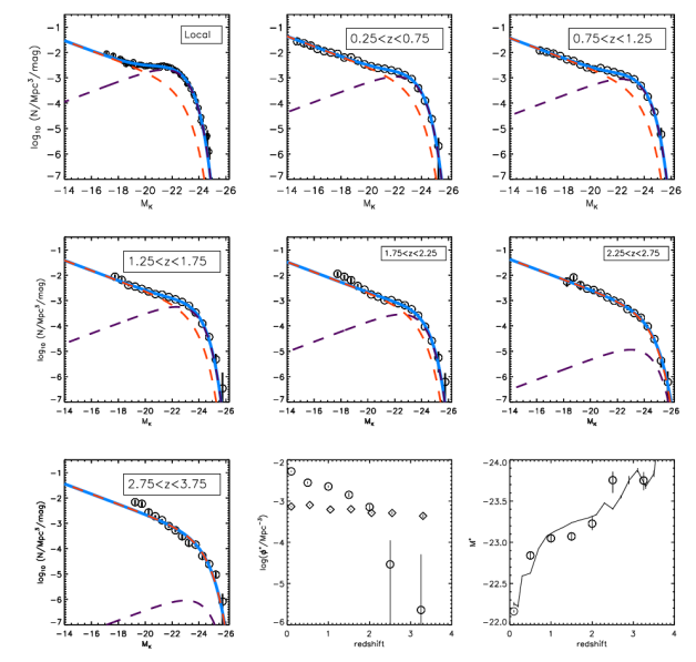
Figure 10: A comparison between our new measurement of the evolving KLF and the best-fitting double Schechter function with a shared value of $M_{K}^{\star}$ and fixed faint-end slopes of $\alpha_{1}=-0.5$ and $\alpha_{2}=-1.5$. In each panel the solid blue line shows the sum of the Schechter function component that dominates at faint magnitudes (red dashed line) and the Schechter function component which dominates the bright end of the KLF at low redshifts (purple dashed line). The top-left panel shows the best-fit to the local KLF dataset under this simplified, 3-parameter prescription. The two panels at the bottom right show the redshift evolution of the three free parameters: $\phi_{1}^{\star}$ (open circles), $\phi_{2}^{\star}$ (diamonds) and $M_{K}^{\star}$. The solid line in the bottom-right panel shows the expected evolution of $M_{K}^{\star}$ if it is assumed to correspond to a constant stellar mass of $M_{\star}\simeq 5\times 10^{10}\mathrm{M_{\odot}}$ at all redshifts (see text for a discussion).

6 A simple prescription for the evolution of the KLF

The analysis of the evolving KLF in the previous section has established two clear facts. Firstly, it is necessary to employ a double Schechter function in order to reproduce the observed KLF at $z\leq 2$. Secondly, the results of separately fitting a double Schechter function to each redshift bin suggest that the evolving KLF can be described by the combination of a smoothly evolving bright-end component and an approximately constant faint-end component.

These conclusions are strengthened further by the left-hand panel of Fig. 9, which shows an overlay of the KLF data from all six redshift bins. This plot gives the impression that if sufficient dynamic range in luminosity were available, the KLF would be observed to have a roughly constant normalisation and faint-end slope at $M_{K}\geq-20$. Moreover, over the redshift interval $0.25\leq z\leq 3.75$ there appears to be surprisingly little evolution, perhaps no evolution, in the number density of the brightest galaxies at $M_{K}\leq-24$. Indeed, over the redshift interval studied here, the left-hand panel of Fig. 9 strongly suggests that the evolution of the KLF largely consists of a smooth build-up in the number density of intermediate luminosity galaxies within the absolute magnitude range $-20\leq M_{K}\leq-24$. Similar results have been found for the UV luminosity function in Bowler et al. (2015).

This scenario immediately suggests that it would be interesting to explore the evolution of the KLF within the context of the phenomenological galaxy evolution model proposed by Peng et al. (2010). The Peng et al. (2010) model describes the total GSMF at $z\leq 2$ as a double Schechter function with a shared value of $M_{\star}\simeq 5\times 10^{10}\mathrm{M_{\odot}}$, the value of which is governed by the process of mass quenching of star formation.

In this model the overall double Schechter-function shape of the GSMF is produced by the combination of an approximately constant star-forming component and a rapidly evolving quenched component. The star-forming component is described by a single Schechter function with a fixed faint-end slope of $\alpha_{SF}\simeq-1.3$, whereas the quenched component has a double Schechter functional form, with a faint-end slope of $\alpha_{SF}$ and a bright-end slope of $\alpha_{Q}=\alpha_{SF}+1$. The combination of star-forming and quenched components produces an overall stellar mass function with a double Schechter functional form with a faint-end slope of $\alpha_{SF}$, a bright-end slope of $\alpha_{SF}+1$ and a shared value of $M_{\star}\simeq 5\times 10^{10}\mathrm{M_{\odot}}$. Observationally, this model is known to be consistent with recent determinations of the GSMF at $z\simeq 0$ (e.g. Baldry, Glazebrook & Driver 2008; Baldry et al. 2012) and $z\simeq 1$ (e.g. Ilbert et al. 2013; Tomczak et al. 2014; Mortlock et al. 2015).

Motivated by this, we explored re-fitting the KLF using a double Schechter function with a shared value of $M_{K}^{\star}$, insisting that the slope of the component describing the faint-end of the KLF ($\alpha_{2}$) is constant with redshift and enforcing the additional constraint that $\alpha_{1}=\alpha_{2}+1$. The adopted value of $\alpha_{2}$ was derived from a fit to the KLF data within the $0.25\leq z\leq 0.75$ redshift bin which covers that largest dynamic range in $K$-band luminosity. By stepping through a grid with a spacing of $\Delta\alpha_{2}=\Delta\alpha_{1}=0.1$, it was determined that ($\alpha_{1},\alpha_{2})=(-0.5,-1.5)$ provided the best-fit and these values were therefore adopted and held constant when fitting the KLF in all six redshift bins. The results of this constrained 3-parameter fitting process are listed in Table 5 and plotted in the right-hand panel of Fig. 9.

In Fig. 10 we compare the results of the constrained KLF fitting to the data in all six redshifts bins, illustrating how the two components combine to provide the overall double Schechter shape. In the top-left panel of Fig. 10 we also show a constrained fit to the local KLF dataset, highlighting that the evolving 3-parameter fit can naturally reproduce the KLF over the full $z=0$ to $z=3.75$ redshift interval. The bottom-right panels of Fig. 10 show the redshift evolution of three free parameters: $\phi^{\star}_{1}$, $\phi^{\star}_{2}$ and $M_{K}^{\star}$.

Interestingly, it can be seen that the normalisation of the Schechter component dominating the faint-end of the KLF ($\phi^{\star}_{2}$) remains approximately constant with redshift, decreasing by a factor of only $\simeq 2$ over a $\simeq 12$ Gyr time-frame. In contrast, the normalisation of the Schechter component that dominates the bright end of the KLF at low redshift ($\phi^{\star}_{1}$) decreases by an order of magnitude between $z=0$ and $z\simeq 2$, before effectively disappearing entirely at $z\geq 2.5$. Moreover, it can be seen from the bottom right panel of Fig. 10 that the shared value of $M_{K}^{\star}$ evolves by $\Delta M_{K}^{\star}\simeq 1.5$ magnitudes, brightening from $M_{K}^{\star}=-22.3$ locally to $M_{K}^{\star}\simeq-23.8$ at $z\simeq 3$.

6.1 Comparison to the stellar mass function

Although this paper is focused on the evolution of the KLF, it is obviously of interest to briefly consider the implications of our simplified description of the evolving KLF in terms of the GSMF.

Recent determinations of the local GSMF have demonstrated that it has a double Schechter functional form, with faint and bright-end slopes which differ by approximately unity. Indeed, in their analysis of the local GSMF using SDSS data, Baldry, Glazebrook & Driver (2008) and Peng et al. (2010) derived values of ($-0.46\pm 0.09$,$-1.58\pm 0.05$) and ($-0.52\pm 0.04$,$-1.56\pm 0.12$) for ($\alpha_{1},\alpha_{2})$ respectively. More recently, Baldry et al. (2012) derived values of ($-0.35\pm 0.17$,$-1.47\pm 0.05$) based on data from the GAMA survey. It is clear therefore that our adopted values of ($-0.5,-1.5$) are in excellent agreement with recent determinations of the local GSMF. Moreover, all three of the local GSMF studies mentioned above derive values of the characteristic stellar mass that are in excellent agreement: $\log({M_{\star}}/{\mathrm{M_{\odot}}})\simeq 10.65\pm 0.01$, $10.67\pm 0.01$ and $10.66\pm 0.05$ respectively (Chabrier 2003 IMF).

Within this context, it is interesting to reconsider the evolution we derive for the characteristic $K$-band magnitude of the KLF based on our constrained 3-parameter fits. In the bottom-right panel of Fig. 10 the solid line shows the expected evolution of the characteristic absolute $K$-band magnitude ($M_{K}^{\star}$), if we make the assumption that it corresponds to a constant stellar mass of $\log({M_{\star}}/{\mathrm{M_{\odot}}})=10.65$. Remarkably, this comparison suggests that the evolution of the KLF between $z=0$ and $z=4$ is perfectly consistent with an evolving value of $M_{K}^{\star}$ which corresponds to a constant stellar mass of $\simeq 5\times 10^{10}\mathrm{M_{\odot}}$ (Chabrier 2003 IMF). Indeed, we note with interest that the latest determinations of the GSMF at $z\geq 4$ suggest that the characteristic stellar mass remains constant at $\simeq 5\times 10^{10}\mathrm{M_{\odot}}$ out to $z\simeq 5$ (Song et al. 2016).

Table 5: The best-fitting double Schechter functions (with fixed faint-end slopes) based on fitting the KLF data shown in Fig. 5 and Table 3. The first column lists the redshift bin and columns $2-6$ list the best-fitting parameters and their corresponding uncertainties. Columns 7 & 8 list the corresponding values of $\chi^{2}$ and reduced $\chi^{2}_{\nu}$ respectively.

Redshift Range	$\log(\phi_{1}^{*}/\rm{Mpc}^{-3})$	$M_{K}^{*}$	$\alpha_{1}$	$\log(\phi_{2}^{*}/\rm{Mpc}^{-3})$	$\alpha_{2}$	$\chi^{2}$	$\chi^{2}_{\nu}$
0.25$<z<$0.75	$-$2.55 ${}^{+0.02}_{-0.03}$	$-$22.84 ${}^{+0.05}_{-0.05}$	$-$0.50 (fixed)	$-$3.10 ${}^{+0.01}_{-0.01}$	$-$1.50 (fixed)	14.7	0.8
0.75$<z<$1.25	$-$2.65 ${}^{+0.03}_{-0.03}$	$-$23.05 ${}^{+0.05}_{-0.05}$	$-$0.50 (fixed)	$-$3.20 ${}^{+0.01}_{-0.01}$	$-$1.50 (fixed)	09.6	0.6
1.25$<z<$1.75	$-$2.85 ${}^{+0.05}_{-0.05}$	$-$23.07 ${}^{+0.05}_{-0.05}$	$-$0.50 (fixed)	$-$3.19 ${}^{+0.01}_{-0.01}$	$-$1.50 (fixed)	06.2	0.5
1.75$<z<$2.25	$-$3.14 ${}^{+0.10}_{-0.10}$	$-$23.23 ${}^{+0.11}_{-0.13}$	$-$0.50 (fixed)	$-$3.29 ${}^{+0.02}_{-0.02}$	$-$1.50 (fixed)	26.9	2.1
2.25$<z<$2.75	$-$4.53 ${}^{+0.58}_{-5.46}$	$-$23.75 ${}^{+0.15}_{-0.10}$	$-$0.50 (fixed)	$-$3.29 ${}^{+0.03}_{-0.03}$	$-$1.50 (fixed)	08.8	0.7
2.75$<z<$3.75	$-$5.39 ${}^{+1.49}_{-4.35}$	$-$23.75 ${}^{+0.21}_{-0.17}$	$-$0.50 (fixed)	$-$3.36 ${}^{+0.04}_{-0.04}$	$-$1.50 (fixed)	30.9	3.1

7 Conclusions

We have presented the results of a study of the evolving KLF, based on a new dataset compiled from the UltraVISTA, CANDELS and HUDF surveys. The large dynamic range in luminosity spanned by this new dataset ($3-4$ dex over the full redshift range) is sufficient to allow a detailed measurement of the functional form of the evolving KLF at $z\geq 1$ for the first time, and to allow a meaningful comparison with the predictions of the latest generation of theoretical galaxy-evolution models. Our principal conclusions are as follows:

1. The large dynamic range in $K$-band luminosity provided by our new dataset is sufficient to demonstrate that the faint-end slope of the KLF is steeper than typically determined by previous $z>0.3$ studies. When fitted with a single Schechter function, our data suggests that the faint-end slope lies in the range $-1.30\leq\alpha\leq-1.54$ within the redshift interval $0.25\leq z\leq 2.75$. Based on a single Schechter-function fit, there is some evidence that the faint-end slope steepens in our final $z\simeq 3.25$ redshift bin ($\alpha=-1.87\pm 0.15$), although the reduced dynamic range in this bin means that the slope is not particularly well constrained.

2. A double Schechter function, with a shared value of $M_{K}^{\star}$, provides a significantly better statistical description of the KLF than a single Schechter function, at least in the redshift range $0.25\leq z\leq 2.25$. At higher redshifts the available dynamic range in luminosity is insufficient to discriminate between a single and double Schechter-function fit.

3. Although significant differences still exist in detail, the overall shape and normalisation of the evolving KLF is found to be in reasonable agreement with the predictions of the latest generation of galaxy-evolution models.

4. Overlaying the data in all six redshift bins suggests that the evolution of the KLF is remarkably smooth. Indeed, the data suggest that the KLF is consistent with having a relatively constant normalisation and slope at faint magnitudes (i.e. $M_{K}\leq-20$) with little, or no, evolution in the number density of galaxies brighter than $M_{K}\leq-24$. Instead, the KLF is observed to evolve rapidly at intermediate magnitudes, with the number density of galaxies at $M_{K}\simeq-23.0$ decreasing by a factor of $\simeq 5$ between $z\simeq 0.25$ and $z\simeq 3.75$.

5. Motivated by the apparently smooth evolution, and the phenomenological model of Peng et al. (2010), we explored the possibility of describing the evolution of the KLF using a double Schechter function with fixed faint-end slopes, such that $\alpha_{1}-\alpha_{2}=1$. Based on fitting the data in our $0.25\leq z\leq 0.75$ redshift bin, which spans the largest dynamic range in luminosity, the best-fitting values of the faint-end slopes were determined to be: $\alpha_{1}=-0.5$ and $\alpha_{2}=-1.5$, in excellent agreement with recent studies of the local GSMF. Moreover, we demonstrated that this ($\alpha_{1},\alpha_{2}$) combination also provides a good description of recent determinations of the local KLF.

6. We find that this simple 3-parameter fit ($M_{K}^{\star},\phi_{1}^{\star},\phi_{2}^{\star}$) provides a remarkably good description of the evolving KLF, in which the normalisation of the component dominating the faint-end remains approximately constant, decreasing by a factor of only $\simeq 2$ over the full redshift range. In contrast, the normalisation of the component dominating the bright end of the KLF at low redshift evolves rapidly, decreasing by an order of magnitude between $z=0$ and $z\simeq 2$ and becoming negligible at $z\geq 2.5$. Moreover, within this framework, the value of the characteristic $K$-band absolute magnitude evolves by $\Delta M_{K}^{\star}\simeq 1.5$ magnitudes, brightening from a local value of $M_{K}^{\star}\simeq-22.3$ to $M_{K}^{\star}\simeq-23.8$ by $z\simeq 3$. This evolution is shown to be entirely consistent with the underlying stellar mass function having a constant characteristic mass of $M_{\star}\simeq 5\times 10^{10}\mathrm{M_{\odot}}$ at all redshifts.

References

- Arnouts et al. (1999) Arnouts S., Cristiani S., Moscardini L., Matarrese S., Lucchin F., Fontana A., Giallongo E., 1999, MNRAS, 310, 540
- Ashby et al. (2015) Ashby M. L. N. et al., 2015, ApJS, 218, 33
- Ashby et al. (2013) Ashby M. L. N. et al., 2013, ApJ, 769, 80
- Baldry et al. (2012) Baldry I. K. et al., 2012, MNRAS, 421, 621
- Baldry, Glazebrook & Driver (2008) Baldry I. K., Glazebrook K., Driver S. P., 2008, MNRAS, 388, 945
- Bell et al. (2003) Bell E. F., McIntosh D. H., Katz N., Weinberg M. D., 2003, ApJS, 149, 289
- Bernardi et al. (2013) Bernardi M., Meert A., Sheth R. K., Vikram V., Huertas-Company M., Mei S., Shankar F., 2013, MNRAS, 436, 697
- Bertin & Arnouts (1996) Bertin E., Arnouts S., 1996, A&AS, 117, 393
- Blanton & Roweis (2007) Blanton M. R., Roweis S., 2007, AJ, 133, 734
- Bouwens et al. (2009) Bouwens R. J. et al., 2009, ApJ, 690, 1764
- Bowler et al. (2015) Bowler R. A. A. et al., 2015, MNRAS, 452, 1817
- Bowler et al. (2014) Bowler R. A. A. et al., 2014, MNRAS, 440, 2810
- Brammer, van Dokkum & Coppi (2008) Brammer G. B., van Dokkum P. G., Coppi P., 2008, ApJ, 686, 1503
- Bruzual & Charlot (2003) Bruzual G., Charlot S., 2003, MNRAS, 344, 1000
- Calzetti et al. (2000) Calzetti D., Armus L., Bohlin R. C., Kinney A. L., Koornneef J., Storchi-Bergmann T., 2000, ApJ, 533, 682
- Caputi et al. (2006) Caputi K. I., McLure R. J., Dunlop J. S., Cirasuolo M., Schael A. M., 2006, MNRAS, 366, 609
- Chabrier (2003) Chabrier G., 2003, PASP, 115, 763
- Cimatti et al. (2002) Cimatti A. et al., 2002, A&A, 392, 395
- Cirasuolo et al. (2010) Cirasuolo M., McLure R. J., Dunlop J. S., Almaini O., Foucaud S., Simpson C., 2010, MNRAS, 401, 1166
- Cirasuolo et al. (2007) Cirasuolo M. et al., 2007, MNRAS, 380, 585
- Cole et al. (2000) Cole S., Lacey C. G., Baugh C. M., Frenk C. S., 2000, MNRAS, 319, 168
- Cole et al. (2001) Cole S. et al., 2001, MNRAS, 326, 255
- Colless et al. (2001) Colless M. et al., 2001, MNRAS, 328, 1039
- Davé, Thompson & Hopkins (2016) Davé R., Thompson R. J., Hopkins P. F., 2016, preprint (arXiv:1604.01418)
- Driver et al. (2011) Driver S. P. et al., 2011, MNRAS, 413, 971
- Driver et al. (2012) Driver S. P. et al., 2012, MNRAS, 427, 3244
- Drory et al. (2003) Drory N., Bender R., Feulner G., Hopp U., Maraston C., Snigula J., Hill G. J., 2003, ApJ, 595, 698
- D’Souza, Vegetti & Kauffmann (2015) D’Souza R., Vegetti S., Kauffmann G., 2015, MNRAS, 454, 4027
- Eke et al. (2005) Eke V. R., Baugh C. M., Cole S., Frenk C. S., King H. M., Peacock J. A., 2005, MNRAS, 362, 1233
- Ellis et al. (2013) Ellis R. S. et al., 2013, ApJL, 763, L7
- Elvis et al. (2009) Elvis M. et al., 2009, ApJS, 184, 158
- Fioc & Rocca-Volmerange (1999) Fioc M., Rocca-Volmerange B., 1999, preprint (arXiv:astro-ph/9912179)
- Fontana et al. (2014) Fontana A. et al., 2014, A&A, 570, A11
- Franx et al. (2000) Franx M. et al., 2000, The Messenger, 99, 20
- Furusawa et al. (2008) Furusawa H. et al., 2008, ApJS, 176, 1
- Galametz et al. (2013) Galametz A. et al., 2013, ApJS, 206, 10
- Gardner et al. (1997) Gardner J. P., Sharples R. M., Frenk C. S., Carrasco B. E., 1997, ApJL, 480, L99
- Genel et al. (2014) Genel S. et al., 2014, MNRAS, 445, 175
- Giavalisco et al. (2004) Giavalisco M. et al., 2004, ApJL, 600, L93
- Glazebrook et al. (1995) Glazebrook K., Peacock J. A., Miller L., Collins C. A., 1995, MNRAS, 275, 169
- Gonzalez-Perez et al. (2014) Gonzalez-Perez V., Lacey C. G., Baugh C. M., Lagos C. D. P., Helly J., Campbell D. J. R., Mitchell P. D., 2014, MNRAS, 439, 264
- Grogin et al. (2011) Grogin N. A. et al., 2011, ApJS, 197, 35
- Guo et al. (2013) Guo Y. et al., 2013, ApJS, 207, 24
- Henriques et al. (2015) Henriques B. M. B., White S. D. M., Thomas P. A., Angulo R., Guo Q., Lemson G., Springel V., Overzier R., 2015, MNRAS, 451, 2663
- Hudelot et al. (2012) Hudelot P. et al., 2012, VizieR Online Data Catalog, 2317
- Ilbert et al. (2009) Ilbert O. et al., 2009, ApJ, 690, 1236
- Ilbert et al. (2006) Ilbert O. et al., 2006, A&A, 453, 809
- Ilbert et al. (2013) Ilbert O. et al., 2013, A&A, 556, A55
- Jarrett et al. (2000) Jarrett T. H., Chester T., Cutri R., Schneider S., Skrutskie M., Huchra J. P., 2000, AJ, 119, 2498
- Jarvis et al. (2013) Jarvis M. J. et al., 2013, MNRAS, 428, 1281
- Jones et al. (2006) Jones D. H., Peterson B. A., Colless M., Saunders W., 2006, MNRAS, 369, 25
- Kelvin et al. (2014) Kelvin L. S. et al., 2014, MNRAS, 439, 1245
- Kocevski et al. (2012) Kocevski D. D. et al., 2012, ApJ, 744, 148
- Kochanek et al. (2001) Kochanek C. S. et al., 2001, ApJ, 560, 566
- Koekemoer et al. (2013) Koekemoer A. M. et al., 2013, ApJS, 209, 3
- Koekemoer et al. (2011) Koekemoer A. M. et al., 2011, ApJS, 197, 36
- Laidler et al. (2007) Laidler V. G. et al., 2007, PASP, 119, 1325
- Lawrence et al. (2007) Lawrence A. et al., 2007, MNRAS, 379, 1599
- Liske et al. (2015) Liske J. et al., 2015, MNRAS, 452, 2087
- Loveday (2000) Loveday J., 2000, MNRAS, 312, 557
- Loveday et al. (2015) Loveday J. et al., 2015, MNRAS, 451, 1540
- Loveday et al. (2012) Loveday J. et al., 2012, MNRAS, 420, 1239
- McCracken et al. (2013) McCracken H. J. et al., 2013, The Messenger, 154, 29
- McCracken et al. (2012) McCracken H. J. et al., 2012, A&A, 544, A156
- McLeod, McLure & Dunlop (2016) McLeod D. J., McLure R. J., Dunlop J. S., 2016, MNRAS, 459, 3812
- McLure et al. (2011) McLure R. J. et al., 2011, MNRAS, 418, 2074
- Merlin et al. (2015) Merlin E. et al., 2015, A&A, 582, A15
- Mobasher, Sharples & Ellis (1993) Mobasher B., Sharples R. M., Ellis R. S., 1993, MNRAS, 263, 560
- Mortlock et al. (2015) Mortlock A. et al., 2015, MNRAS, 447, 2
- Moster et al. (2011) Moster B. P., Somerville R. S., Newman J. A., Rix H.-W., 2011, ApJ, 731, 113
- Nonino et al. (2009) Nonino M. et al., 2009, ApJS, 183, 244
- Oke & Gunn (1983) Oke J. B., Gunn J. E., 1983, ApJ, 266, 713
- Parsa et al. (2016) Parsa S., Dunlop J. S., McLure R. J., Mortlock A., 2016, MNRAS, 456, 3194
- Peng et al. (2010) Peng Y.-j. et al., 2010, ApJ, 721, 193
- Pozzetti et al. (2003) Pozzetti L. et al., 2003, A&A, 402, 837
- Retzlaff et al. (2010) Retzlaff J., Rosati P., Dickinson M., Vandame B., Rité C., Nonino M., Cesarsky C., GOODS Team, 2010, A&A, 511, A50
- Rieke et al. (2009) Rieke G. H., Alonso-Herrero A., Weiner B. J., Pérez-González P. G., Blaylock M., Donley J. L., Marcillac D., 2009, ApJ, 692, 556
- Sanders et al. (2007) Sanders D. B. et al., 2007, ApJS, 172, 86
- Saracco et al. (2006) Saracco P. et al., 2006, MNRAS, 367, 349
- Schinnerer et al. (2007) Schinnerer E. et al., 2007, ApJS, 172, 46
- Smith, Loveday & Cross (2009) Smith A. J., Loveday J., Cross N. J. G., 2009, MNRAS, 397, 868
- Song et al. (2016) Song M. et al., 2016, ApJ, 825, 5
- Steinhardt et al. (2014) Steinhardt C. L. et al., 2014, ApJL, 791, L25
- Tomczak et al. (2014) Tomczak A. R. et al., 2014, ApJ, 783, 85
- Windhorst et al. (2011) Windhorst R. A. et al., 2011, ApJS, 193, 27
- Wuyts et al. (2011) Wuyts S. et al., 2011, ApJ, 738, 106