Structure and Physical Conditions in the Huygens Region of the Orion Nebula

Abstract

HST images, MUSE maps of emission-lines, and an atlas of high velocity resolution emission-line spectra have been used to establish for the first time correlations of the electron temperature, electron density, radial velocity, turbulence, and orientation within the main ionization front of the nebula.

From the study of the combined properties of multiple features, it is established that variations in the radial velocity are primarily caused by the photo-evaporating ionization front being viewed at different angles.

There is a progressive increase of the electron temperature and density with decreasing distance from the dominant ionizing star $\theta^{1}$ Ori C. The product of these characteristics (n_e$\times$ T_e) is the most relevant parameter in modeling a blister-type nebula like the Huygens Region, where this quantity should vary with the surface brightness in H$\alpha$.

Several lines of evidence indicate that small-scale structure and turbulence exists down to the level of our resolution of a few arcseconds.

Although photo-evaporative flow must contribute at some level to the well-known non-thermal broadening of the emission lines, comparison of quantitative predictions with the observed optical line widths indicate that it is not the major additive broadening component.

Derivation of T_e values for H⁺ from radio+optical and optical-only ionized hydrogen emission showed that this temperature is close to that derived from [N ii] and that the transition from the well-known flat extinction curve that applies in the Huygens Region to a more normal steep extinction curve occurs immediately outside of the Bright Bar feature of the nebula.

1 introduction

The basic model of the Huygens Region of the Orion Nebula is that of an irregular concave blister of ionized gas located on the observer’s side of a giant molecular cloud (a summary is found in (O’Dell, 2001)). van der Werf & Goss (1989) established through observations of the HI 21 cm line in absorption that there was a foreground Veil of primarily neutral material. The Veil has been the subject of several additional studies using radio and optical absorption lines (van der Werf et al., 2013; Abel et al., 2016). These studies refine the properties of the Veil, although its distance from the dominant ionizing star ($\theta^{1}$ Ori C) remains uncertain. The study of the correlation of HI absorption and reddening by O’Dell et al. (1992) established that the extinction of the nebula and the Trapezium stars arise within the foreground Veil. Within the space between the concave blister of ionized gas and the Veil, there is a molecular cloud called Orion-South (sometimes Orion-S) which is ionized on the observer’s side, but molecular absorption lines indicate that it lies in front of another layer of ionized gas. Within the volume between $\theta^{1}$ Ori C and the Veil there is a blue-shifted layer of ionized gas (the Blue Layer) whose origin and properties are uncertain.

The gas density within the blister of gas near the Main Ionization Front (MIF) decreases rapidly with increasing distance from the MIF (towards the observer). This ionized gas is stratified in ionization, each layer having an easily observed strong emission line. [O i] emission arises from immediately at the MIF. Closer to $\theta^{1}$ Ori C there is a layer of He^o+H⁺ giving rise to [N ii] emission. This layer is about 1″ thick (O’Dell, 2001). That layer gives way to the higher ionization He⁺+H⁺ layer , which is about 30″ thick (O’Dell, 2001), and produces strong [O iii] emission. The Balmer lines (H$\alpha$ and H$\beta$) arise from both layers. $\theta^{1}$ Ori C is too cool to produce a higher ionization layer.

The brightest portion of the Orion Nebula (M 42, NGC 1976) is commonly designated as the Huygens Region, as it was first depicted in print by Christiaan Huygens in the mid 17th century (Gingerich, 1982). The Huygens Region has been the subject of many studies at essentially all available energies, but defies a definitive resolution of its structure and physical conditions. Recent reviews (Muench, et al., 2008; O’Dell et al., 2008) describe in more detail our knowledge of the nebula and its associated young stars.

Although the basic model of the nebula seems to be understood, there are many unresolved issues. What is the cause of the variations in radial velocity across the face of the nebula? Is there evidence for small-scale variations in the electron temperature? What is the cause of the known electron density and electron temperature variations? What is the source of the unexpected width of the emission lines? This list could be continued, but the important bottom-line is that the Huygens Region of the Orion Nebula is our best opportunity for studying other H II regions, both in our Galaxy and in extragalactic systems; if we cannot understand the processes occurring in this object, conclusions about other similar but more poorly characterized objects are rendered correspondingly uncertain.

In this article we report on an investigation of the physical conditions within the Huygens Region and how these relate to features near the MIF. Such an investigation was made possible through the existence of an atlas of high velocity resolution (García-Díaz et al., 2008) (hereafter the Spectral Atlas), numerous Hubble Space Telescope images, and a recent moderate resolution spectroscopic map (Weilbacher et al., 2015). In Section 2 we describe the data used and their processing. In Section 3 we describe the basic premise in interpretation of the radial velocities. In Section 4 we present the study of individual features and regions and how this reveals their structure and physical conditions. In Section 5 we explore the variations of n_e, T_e, and structure in the eastern region of the Orion-South Cloud, which contains multiple high velocity jets and shocks. In Section 6.1 we discuss the meaning of the observed large values of the Full Width at Half Maximum (FWHM). A summary of the results of relating T_e to other nebular characteristics is in Section 6.2. What the lack of a back-scattered component tells us about the 3-D structure of some samples is presented in Section 6.3. The results of an attempt to determine T_e for H⁺ is given in Appendix A. A summary of this study is presented in Section 7.

2 The data sets employed

2.1 Imaging Data

The Huygens Region  was a natural target for one of the first observations with the MUSE moderate resolution spectrograph (Weilbacher et al., 2015). We draw heavily upon this data-set, which generously is in the public domain.The images were reprocessed, using the original images, as described in our paper on fine scale temperature fluctuations in the Huygens Region (William Henney, et al., in preparation). Although the fiber optics defining the sampling has a size of 0$\aas@@fstack{\prime\prime}$2 over the 353$\aas@@fstack{\prime\prime}$2$\times$295$\aas@@fstack{\prime\prime}$2 Field of View (FOV), the images created are about 1″ FWHM. A shortcoming of this data set is that only a single exposure time was used for each pointing, so that the signal to noise (S/N) ratio decreases as one utilizes the weaker lines. For our study, we employed only strongest lines (486.1 nm, H$\beta$; 500.7 nm, [O iii]; 656.3 nm, H$\alpha$; 658.3 nm, [N ii]). The derivation of T_e was done using both the strong 658.3 nm nebular line and the weaker 575.5 nm auroral line, while n_e was determined from the moderately strong red [S ii] doublet (671.6 nm and 673.1 nm). Throughout this paper we will use the T_e and n_e values determined by Henney, et al. Unfortunately, the low velocity resolution (107 km s^-1) of the MUSE spectra preclude study of any but the highest radial velocity (V_r) features.

Although monochromatic images can be made of the full MUSE field of view, the superior resolution HST images were employed where possible. The original mosaic of images using the lower resolution WFPC2 camera images (O’Dell & Wong, 1996) were frequently employed, although in a few cases the better sampled PC camera images were available (O’Dell et al., 1997). The HST images (about 0$\aas@@fstack{\prime\prime}$08)were calibrated into flux units using the calibration constants determined by comparing regions within these images with flux calibrated ground-based telescope observations (O’Dell, 2009a). For our purposes it was sufficient to ignore the low level of contamination of the HST emission-line filters by the underlying continuum and for contaminating lines falling in the wings of the filters.

2.2 Spectra

The high velocity resolution spectra we used are from the Spectral Atlas compiled by García-Díaz et al. (2008). These have a velocity resolution of about 8–10 km s^-1. The Spectral Atlas was compiled from a series of north-south oriented slit spectra made with a spacing of 2″ under conditions of astronomical seeing better than that. This means that the Spectral Atlas has a spatial resolution of about 2″. Although the Spectral Atlas includes incomplete mapping in additional lines, we employed only the fully mapped [O iii] 500.7 nm and [N ii] 658.3 nm lines, which were calibrated to about 2 km s^-1 accuracy.

These high S/N spectra of [O iii] and [N ii] are intrinsically narrow and can be de-convolved into multiple components. This was not possible with the ubiquitous H$\alpha$ and H$\beta$ lines because of their large thermal width. As done in earlier studies of the Huygens Region de-convolution was done by using the IRAF task "splot". In addition to the strongest component (produced on the observer’s side of the MIF) there is almost always a red wing of about 10% the strength of the MIF component (produced by backscattering from the dust in the compressed neutral zone beyond the MIF), and often a weaker blue component. The V_r of the MIF component could usually be determined with an accuracy of 1 km s^-1 or better, while the accuracy of the red and blue radial velocities are about 3 km s^-1, the exact value depending on the flux relative to the MIF and the velocity separation from that same strong component. The origin of the red component as backscattered light is by now well established (O’Dell et al., 1992; Henney, 1994; O’Dell, 2001; Abel et al., 2016) as it is fully consistent with the blister model for the MIF and the photo-evaporation velocity shift between the emitting and scattering layers produces a doubling of the observed velocity separation. One would expect that the relative strength of the backscattered component to be weak compared with the MIF component when seeing a highly tilted portion of the MIF. The few absences of a backscattered component are discussed in Section 6.3. The more difficult to observe blue component is best described as a layer of ionized gas lying between $\theta^{1}$ Ori C and the foreground Veil (Abel et al., 2016).

3 Interpretation of variations of the MIF Radial Velocities

The radial velocities of the MIF components are particular important in studying the inclination of the local MIF. For a photo-evaporating blister nebula gas is ionized at the MIF, then flows away from the Photo Dissociation Region (PDR). The [N ii] emission arises from closer to the MIF and has a smaller (blueshifted) velocity relative to the PDR than the [O iii] emission, which is from gas that has been accelerated more as it reaches a larger distance from the MIF. Observations of [C ii] (Goicoechea, 2015) at a spatial resolution of about 11$\aas@@fstack{\prime\prime}$4 indicate that the V_r of the PDR (which gives rise to the [C ii] emission) is constant at 27.5$\pm$1.5 km s^-1(LSR) across the Huygens Region and are indistinguishably the same as the average of the lower spatial resolution CO velocities (27.3$\pm$0.3 km s^-1 LSR (derived from Table 3.3 VII of Goudis (1982). If the MIF was at a fixed angle with respect to the sky, then one would expect V_r for [O iii] and [N ii] to be constant, with [O iii] more blueshifted than [N ii]. However the observed V_r varies for both lines across the Huygens Region. For a face-on MIF the observed V_r would be V_PDR - V_exp, where V_PDR is the velocity of the PDR and V_exp is the photo-expansion velocity. In the case of the MIF being viewed edge-on, the observed V_r would be V_PDR, since the V_exp component will then be perpendicular to the line of sight. Throughout this paper we will interpret variations in the observed V_r as due to variations in the tilt of the MIF.

4 Areas and Features Discussed in Detail in this Paper

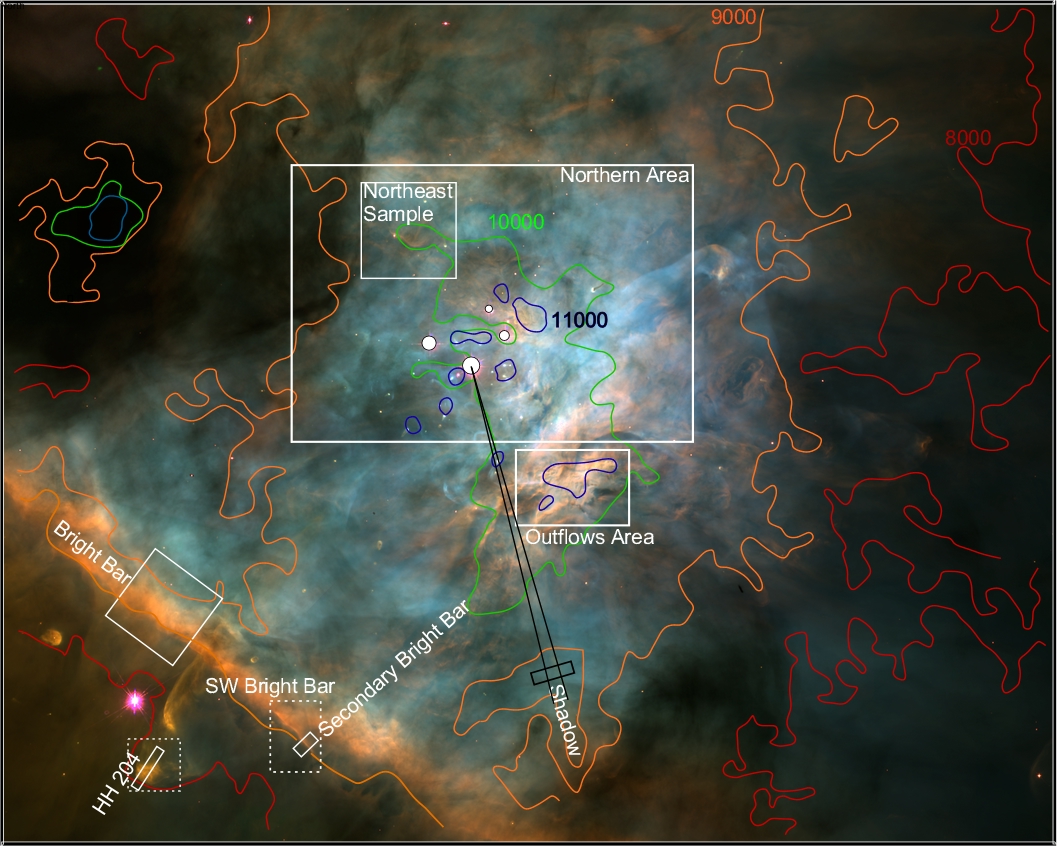
Figure 1: This 204$\aas@@fstack{\prime\prime}$2$\times$243$\aas@@fstack{\prime\prime}$6 FOV image of the Huygens Region of the Orion Nebula is taken from a mosaic of WFPC2 HST images (O’Dell & Wong, 1996), where the colour coding is Blue-F502N ([O iii]), Green-F656N (H$\alpha$), and Red-F658N ([N ii]) and is slightly smaller than the MUSE (Weilbacher et al., 2015) FOV. The colour contours are the [N ii] T_e values derived from our processing of the MUSE data (W. J. Henney-in preparation). Rectangular boxes indicate features discussed in various sections of the text. The two lines extending from the brightest star ($\theta^{1}$ Ori C, 5:35:16.46 -5:23:22.9) in the Trapezium grouping indicate the alignment with obscuring material that defines the ionization shadow discussed in Section 4.5. One dashed box indicates the fine-structure portion of the Bright Bar that we designate as the SW Bright Bar. The other dashed box indicates the region around HH 204 studied by Núñez-Diaz et al. (2012).

We have sampled multiple regions within the Huygens Region, as illustrated in Figure 1. They were selected to cover a variety of characteristics. HH 204 (Section 4.1) is a well defined shock structure seen to advantage against the much lower surface brightness of the nebula outside of the Bright Bar. Linear features are studied in the region of the Bright Bar (Section 4.2), the SW Bright Bar (Section 4.3), and within an ionization shadow (Section 4.5), with the former two represented regions where the MIF is viewed almost edge-on. Within the Northern Region there is a large high T_e arcuate structure (Section 4.4) that is a structure within the MIF in spite of its resemblance to a bow shock. The complex Northern Region is discussed in Section 4.6 where the effect of local variations in structure of the MIF are illuminated. Finally, the regions of multiple high velocity outfows are discussed in Section 5.

4.1 HH 204

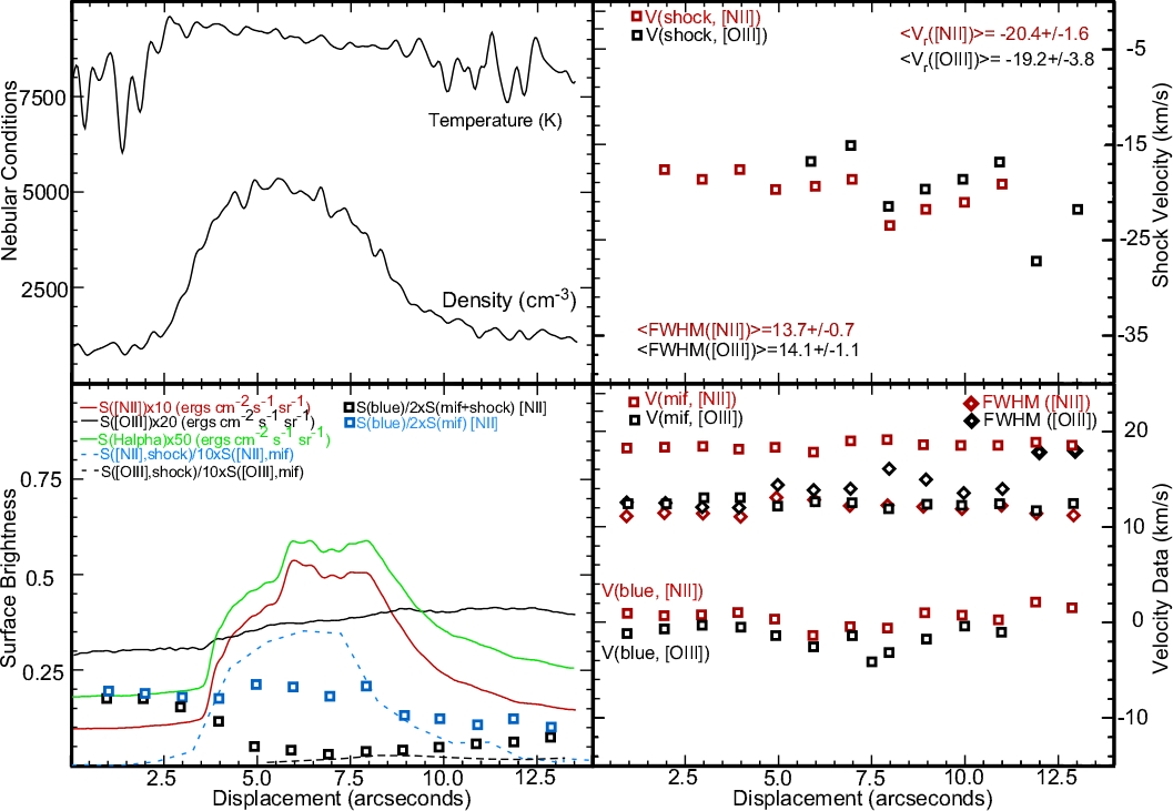
Figure 2: This figure shows various quantitative results derived for the sample marked HH 204 in Figure 1. Given the large amount of data and the need to compress its presentation, in some cases the data has been scaled. Increasing displacement corresponds to displacement along the shock towards PA = 327°.

There is a rich literature of observations of the object now designated as HH 204. It has been imaged at highest resolution with the PC camera of the HST (O’Dell et al., 1997), its motion in the plane of the sky has been determined (Doi, O’Dell, & Hartigan, 2002), and its V_r mapped at high spectral resolution (Doi, O’Dell, & Hartigan, 2004). Mesa-Delgado et al. (2008) obtained a long-slit spectrum along the axis of symmetry of the shock and a region of 15″ $\times$ 15″  at the apex was mapped with 1″, pixels with integral field spectroscopy of 3.5 Å resolution (Núñez-Diaz et al., 2012). In spite of this variety of studies, more can be done, especially with the use of high velocity resolution data.

The HH 204 shock is driven by a high velocity jet originating near the eastern side of the Orion-South molecular cloud. The most recent discussion of the probable origin is found in O’Dell et al. (2015). The shock moves toward the observer with a spatial velocity of 103 km s^-1 at an angle of about 27° out of the plane of the sky (Henney, 2007). It is unclear if it is formed as the jet strikes the foreground Veil (O’Dell et al., 1997) or the raised escarpment that produces the Bright Bar (Doi et al., 2004; van der Werf et al., 2013). It is pointed away from $\theta^{1}$ Ori C and its structure is consistent with a shock that is photoionized from within, that is, the material within the parabolic envelope of the shock is illuminated and ionized by $\theta^{1}$ Ori C.

We created a sample along the slit spectrum of Mesa-Delgado et al. (2008) and within the area studied by Núñez-Diaz et al. (2012). Our sample is 2$\aas@@fstack{\prime\prime}$4 wide and 13$\aas@@fstack{\prime\prime}$5 long. The physical conditions were sampled from the [S ii]-derived n_e and [N ii]-derived T_e  approximately 1″ resolution maps using the MUSE data. The results are shown in the top-left panel of Figure 2 and are similar the results presented in Figure 7 of Núñez-Diaz et al. (2012). It should be noted that the zero-point of our samples is at -3$\aas@@fstack{\prime\prime}$2 on the Núñez-Diaz et al. (2012) plot. Higher spatial resolution (about 0$\aas@@fstack{\prime\prime}$1) samples of the surface brightness were made using the calibrated WFPC2 images of [N ii], H$\alpha$, and [O iii]. These are shown in the lower left panels of Figure 2. It should be noted that the WFPC2 filters would have transmitted both the MIF and the highly blueshifted components.

The same sampling was done using the [N ii] and [O iii] lines from the Spectral Atlas. In this case the sampling distance was 0$\aas@@fstack{\prime\prime}$5 (however, recall that the spacing of the Spectral Atlas North-South slits is 2″ while the sampling in each line is 0$\aas@@fstack{\prime\prime}$53 and characteristic seeing was about 2″) and each of these pseudo-spectra samples of 2$\aas@@fstack{\prime\prime}$4$\times$0$\aas@@fstack{\prime\prime}$5 was de-convolved using "splot". As presented in Section 2, the Huygens Region spectra usually de-convolve into the MIF, Red (backscattered), and Blue (an ionized layer). In addition to these three components, we also saw a much more blueshifted component arising in shocked gas. The radial velocities for the shocked components are shown in the top-right panel of Figure 2, in addition to the average of the FWHM of these shock components. The average FWHM values are only slightly larger than those for the individual samples of the MIF components, as shown in the lower-right panel. The shocked material velocities are well blueshifted with respect to the MIF velocities shown in that same lower-right panel. The blue component velocities in the lower-right panel are at values similar to much of the rest of the nebula (0.9$\pm$2.8 km s^-1 for [O iii] and 1.8$\pm$1.9 km s^-1 for [N ii], (Abel et al., 2016)).

In this object and the other subsequent objects addressed we have adopted a procedure to assure that the slit spectra samples align with the images used to produce n_e, T_e, and emission-line profiles. We created from the spectra the total surface brightness at each slit. The total surface brightness includes all of the components of the line. The sequence of slits was shifted to provide agreement of the image profile (the filters are wide enough to include emission from all the velocity components) and the results from the spectra.

The abrupt drop in S([N ii]) and S(H$\alpha$) at 3$\aas@@fstack{\prime\prime}$5 indicates that there is an ionization boundary associated with the shock, as argued in Núñez-Diaz et al. (2012). At that same point we see S([O iii]), drop slightly from an enhanced level to what must be the nebular background level. This supports the argument that the envelope of the shock is photoionized from the inside by $\theta^{1}$ Ori C. The density (rising to 4000 cm^-3 over ambient) agrees in location with the S([N ii]) and S(H$\alpha$) increase over 3″–9″.

We also give the ratio of surface brightness of the shocked over the MIF components (the dashed lines) in the lower-left panel of Figure 2. We see there that the [N ii] shock component reaches 3.6 times the strength of the MIF component and that the [O iii] shock component reaches only 0.3 times the strength of the MIF component. The WFPC2 image of [O iii] has a much higher S/N ratio and the fact the the total surface brightness in [O iii] determined from that data extends to the shock boundary defined by the drop in S(H$\alpha$) and S([N ii]) means that shocked [O iii] material fills the envelope of the shock all of the way to the ionization boundary. In addition, the dominance of shocked [N ii] beyond the ionization boundary indicates that it is shocked gas producing the density jump.

Not only do we confirm the model for HH 204 presented by Núñez-Diaz et al. (2012), we also confirm that there is a narrow zone of high T_e material just outside of what one would ordinarily call the ionization boundary. The biggest step in the present study is the use of high velocity spectra to clearly link the T_e and n_e enhancements to the shocked material.

The blue component (whose velocities are well separated from those of the MIF and the shocks) is unusually strong. In the samples of Abel et al. (2016) they found that the Blue/MIF surface brightness ratio was about 0.08$\pm$0.04. In the lower-left panel of Figure 2 we see that the observed ratio varies greatly, depending on whether one is taking as the denominator the sum of the MIF and Shock components or the MIF component alone. It is most likely that the ratio using only the MIF component is relevant and its ratio is nearly constant along the sample (an average of 0.31$\pm$0.09). This indicates that the Blue Layer is independent of the HH 204 shock. However, it is probably significant that the ratio of the Blue/MIF components in this sample (all outside of the Bright Bar) is some four times larger than the central nebula samples of Abel et al. (2016) and rises in our HH 204 sample with increasing distance from the Bright Bar. As we shall see in Section A.4, there are arguments for abrupt changes in the foreground material as one goes beyond the Bright Bar.

4.2 The Bright Bar

The feature known as the Bright Bar is well studied and beyond the fact that it is basically an escarpment viewed nearly from along the cliff face it is not well understood, both at a fine-scale (Is it a simple curved surface or an undulating surface viewed almost edge-on?) and at a large scale (How does one produce a structure in the MIF that is so linear?). Listings of the arguably best earlier studies of the ionized side (facing $\theta^{1}$ Ori C) and neutral side (mostly molecules) are presented in (Walmsley, 2000; O’Dell et al., 2008). More recently there have been additional valuable observational studies (van der Wiel et al., 2009; Mesa-Delgado et al., 2011) and models (Henney, 2005b; Pellegrini et al., 2009; Shaw et al., 2009; Ascasibar et al., 2011). García-Díaz & Henney (2007) present evidence for several other bar structures, but none are as obvious as the Bright Bar. In this study we have sought to bring together the recently available MUSE material, the high velocity resolution Spectral Observations material, and HST optical imaging to produce a more accurate picture of what it is.

In order to obtain high S/N data, we have grouped the data within the Bright Bar sample box (Figure 1 into narrow samples parallel (PA = 53.4°) to the Bright Bar. Each sample was 24″ long and the artificial spectra was created similar to the study of HH 204 and have a spacing of 1″. There is a certain amount of averaging along each sample because of the fine-scale structure of the Bright Bar. This reduces the inherently high resolution of the HST images but probably does not change the 2″ resolution inherent in the Spectral Atlas. The MUSE data of about 1″ resolution was probably degraded slightly by this process, but not by much.

We present our results in the middle three panels of Figure 3. The vertical dashed reference line shows the position of the peak surface brightness in [N ii] S([N ii]). The top panel shows the variation in T_e (from [N ii]) and n_e (from [S ii]) as derived from our treatment of the MUSE data. In the middle panel we show most of our results from the [N ii] spectra and the lowest panel shows the profile of the surface brightness in [N ii] and [O iii].

In the top panel we see that T_e begins at 8800$\pm$100 K on the northwest side and peaks at 9100$\pm$50 K at 2″ beyond the S([N ii]) peak, then drops to 8700$\pm$100 at the end of the samples. In contrast, the n_e begins at 2000$\pm$50 cm^-3 and rises to 3400$\pm$100 cm^-3 about 1$\aas@@fstack{\prime\prime}$5 inside the S([N ii]) line, then, descends to 1600$\pm$50 cm^-3.

Since the [N ii] emitting layer is much thinner than the [O iii] layer, we only present the results from using ’splot" to de-convolve the [N ii] 658.3 nm line, the results of this appearing in the middle panel. Within the paradigm that variations in radial velocity of the MIF are due to variations in the tilt we can interpret the slow increase in V_r([N ii]) as an increase in the tilt passing a peak at 2″ beyond the S([N ii]) peak, then dropping abruptly, and assuming a constant lower tilt 3″ beyond the S([N ii]) peak. On the inside of the Bright Bar V_r([N ii]) is 22.5 km s^-1, rising to a maximum at the Bright Bar peak of 23.6 km s^-1, then dropping to 18.2 km s^-1 outside the Bright Bar.

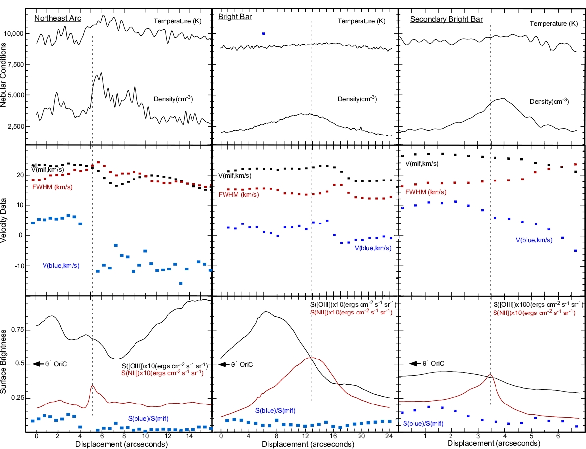
Figure 3: The results of profiles taken across different samples are shown as a function of increasing distance from the end of the sample closest to $\theta^{1}$ Ori C. The top panels show the profile of T_e and n_e. The middle panels show the results of using ’splot’ to de-convolve the [N ii] spectra, presenting V_r, FWHM, and V_r of the blue component. The lowest panels show flux calibrated surface brightnesses as derived from HST images and the ratio of surface brightness of the blue component to that arising from the red component. In left to right order these data are discussed in Section 4.4, Section 4.2, and Section 4.3 respectively.

4.2.1 3-D structure determined from V_r([N ii])

If the [N ii] expansion velocity is 10 km s^-1(Section 3 and if the average V_r for [C ii] and CO is 27.4 km s^-1 (Section 3) is representative of the velocity of the underlying molecular cloud, then the inner region is tilted 57°, the Bright Bar 71°  and the outer region 26° with respect to the plane of the sky. This means that the inner region is already quite tilted and the Bright Bar is only a locally greater tilt. The outer region is the least tilted. These values are very sensitive to the adopted expansion velocity, which is less certain than the molecular cloud velocity.

If one assumes that the outer region is in the plane of the sky, then V_exp([N ii]) would 9.2 km s^-1 rather than 10 km s^-1and the tilt inside the Bright Bar would be 53° and the Bright Bar 68° with respect to the plane of the sky. If the [N ii] expansion velocity is the minimum value of 9.2 km s^-1, the angles would be 33°, 24°, and 90° respectively. If the [N ii] expansion velocity is greater than 10 km s^-1 then the angles would all be smaller.

The inner region being highly tilted agrees with the 3-D model for the inner Huygens Region constructed by Wen & O’Dell (1995) from measurements of the radio continuum surface brightness and densities derived from the [S ii] red doublet. The tilt at the Bright Bar’s peak is less than that given in studies of comparing model ionized slabs with the observations and these differences are probably due to the expansion velocity used and a break-down of the assumed model in a region of rapidly changing tilt. The tilt of the MIF outside the Bright Barmust not be as large as 90° because the outer parts of the nebula would be shielded from the ionizing radiation from $\theta^{1}$ Ori C. In fact, the shape of the inner Huygens Region must be determined by the photo-evaporation of material through the MIF as it eats its way into the host molecular cloud.

4.2.2 What the sequence of characteristics tells us about the 3-D structure of the Bright Bar

We have a small but clear sequence of properties across our Bright Bar sample. The peak in n_e occurs at 12$\aas@@fstack{\prime\prime}$0 from the $\theta^{1}$ Ori C end of the sample, the S([N ii]) peak occurs at 12$\aas@@fstack{\prime\prime}$8, the maximum T_e occurs at 15″, and the change of velocity characteristics V_r([N ii]) and FWHM occurs at 17″. It should be recalled that all of these characteristics are derived from [N ii] observations except for n_e, which is derived from observations of [S ii].

The most straightforward interpretation is that the n_e peak occurs within an He^o+H⁺ layer viewed almost edge-on along a line-of-sight where there is the most favorable combination of events producing [S ii] emission (i.e. the ionic abundance of S ⁺, n_e, and T_e). The S([N ii]) peak would be along a line-of-sight where most favorable combination of density of n_e, N ⁺, and T_e occur. The inner part of this He^o+H⁺  layer would have the highest total gas density as material is photo-evaporated away from the ionization boundary of the MIF. The T_e maximum would occur in the level of the He^o+H⁺ layer where conditions for emitting [N ii] are best and also where the local T_e is rising because of radiation hardening that occurs as one approaches the MIF and the increase of the gas density. Finally, the local peak in V_r([N ii]) and FWHM marks the point of inflection, where the He^o+H⁺ layer tilt changes abruptly. However, the expected relation between V_r and FWHM (FWHM is larger where V_r is smaller) is not seen.

4.2.3 The Blue Layer emission near the Bright Bar

The Blue Layer V_r changes abruptly at about 2″ inside the position of the drop in V_r([N ii]). This argues that the Blue Layer is different on the two sides of the Bright Bar. The Blue Layer component surface brightness mimics that of S([N ii]) as one sees in the lowest panel, where S(blue)/S(mif) does not change significantly when crossing the S([N ii]) maximum. However the maximum Blue Layer surface brightness [S([N ii])$\times$S(blue)/S(mif)] peaks at 13$\aas@@fstack{\prime\prime}$5, near where V_r(blue) peaks before dropping further out.

This article cannot give a definitive answer about the origin, location, and nature of the Blue Layer even though it adds to the body of knowledge about this feature. A more comprehensive paper is in preparation by co-author O’Dell.

Figure 4: This 14$\aas@@fstack{\prime\prime}$5$\times$20$\aas@@fstack{\prime\prime}$4 field is designated as the SW Bright Bar in Figure 1. The colour coding is the same as in that figure, although the colour balance is slightly different. A 4$\aas@@fstack{\prime\prime}$0 sample along the linear portion in the southwest portion of this image was used in the study presented in the right-hand panels of Figure 3.

4.3 A SW Bright Bar Narrow Feature

In Figure 1 we designate as the SW Bright Bar that section of the Bright Bar that is distinctly different. In this smaller region there is a wavy narrow feature that looks like a sharp ionization front that we designate as the Secondary Bright Bar. We have sampled a linear portion of this feature by a series of 0$\aas@@fstack{\prime\prime}$5 samples 4$\aas@@fstack{\prime\prime}$0 wide with PA = 54°, with the resulting profiles shown in the right hand panels of Figure 3. The centre of the sharp feature, seen best in Figure 4 is at 5:35:19.64 -5:25:12.1.

One has to bear in mind in examining the profile of V_r, FWHM, and V_r(blue) that these were made from spectra with a spatial resolution of about 2″ whereas the other data have better resolution (n_e and T_e about 1″ and the surface brightness data about 0$\aas@@fstack{\prime\prime}$1).

The distribution of S([N ii]) is similar to that of the Bright Bar, but the peak is much sharper, which is quite consistent with Figure 1 that shows the feature to be the narrowest structure along the Bright Bar. The S([O iii]) variation is similar to that of the Bright Bar in that it is more diffuse and peaks closer to the end of the sample facing $\theta^{1}$ Ori C. The S([N ii]) peak argues that we are seeing an ionization front almost edge-on. Unlike the Bright Bar both T_e and n_e peak beyond the S([N ii]) peak at 3$\aas@@fstack{\prime\prime}$9. The density peak of 4700 cm^-3 rises above the background of 2700 cm^-3. The T_e peak of 9800$\pm$200 K lies above the closer region value of 9400$\pm$200 K and the further region value of 9000$\pm$200 K.

However, the V_r([N ii]) distribution disagrees with the model presented in the previous paragraph. The peak value (27.1 km s^-1at 1$\aas@@fstack{\prime\prime}$2) is well inside the S([N ii]) peak and V_r decreases along the sample. The peak velocity is almost the same as our adopted PDR velocity of 27.4 km s^-1 and this indicates that the inner sample of the MIF is viewed almost edge-on and further from this peak the MIF is flattening. The most likely interpretation of the contradiction of the surface brightness, density, and temperature with the radial velocity data is that the dynamic model (V_r is determined by the tilt of the MIF) has broken down at this small scale and location. We also see an indication of this breakdown in that the inner FWHM is comparable to the inner FWHM in the Bright Bar samples, even though V_r is much higher. Although the V_r and FWHM values vary inversely with one another, in the outermost samples the FWHM has become larger. This is again unlike the Bright Bar.

In contrast with almost all the other regions sampled, any backscattered red component is too weak to be detected. Although this is expected when one looks at an edge-on ionization front, in this case the absence is on both sides of the S([N ii]) peak. Another thing to be noted is that the large displacement V_r(blue) values are well-defined and measured accurately by ”splot”, but in the lower displacement samples the ”splot” values plotted in Figure 3 are too large, as visual examination of the spectra indicates that those velocities should be about -3 km s^-1.

The Blue Layer emission velocity is the highest among our samples then drops down to nearly the lowest velocity in our samples. There is a general decrease (left to right) in the [N ii]S(blue)/S(mif) components, but there is a local rise immediately outside the S([N ii]) peak. In summary, the Blue Layer emission behaves very much like the Bright Bar in terms of a change of V_r and S(blue)/S(mif).

4.4 The Northeast Sample

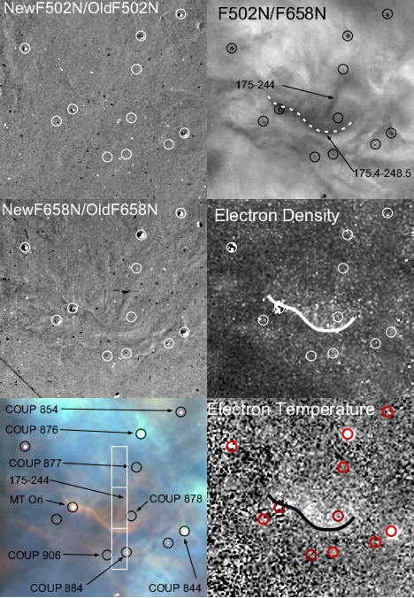
Figure 5: The 26$\aas@@fstack{\prime\prime}$9$\times$25$\aas@@fstack{\prime\prime}$9 Northeast Sample region (Figure 1) that includes the Northeast Arc (traced with curved lines in the right hand panels is shown in multiple depictions as labeled. The colour coding in the bottom left panel is the same as in Figure 1. The other panels are explained and discussed in Section  4.4. The open circles are proplyds, that are characterized by high n_e, high T_e, and low F502N/F658N. The box in the bottom left panel shows the location of the series of 2$\aas@@fstack{\prime\prime}$0 samples at 0$\aas@@fstack{\prime\prime}$5 intervals taken and detailed in Figure 3.

We note in the maps of higher T_e  that to the northeast of the Trapezium is a well defined arc, which we designate here as the Northeast Arc (NE-Arc). This feature falls within the Northeast Sample within Figure 1 and is shown in detail in Figure 5. Although distinctive, it has not attracted previous attention. The southernmost position of the NE-Arc is at 5:35:17.54 -5:22:48.5, which leads to its position based designation (O’Dell et al., 2015) as 175.4-248.5.

In Figure 5 we show the region around the NE-Arc. The lower left and upper right panels show that the feature is low ionization ([N ii] is strongest) and that it encloses a 5$\aas@@fstack{\prime\prime}$9 linear low ionization feature designated as 175-244. We note that the enhanced n_e and T_e regions fall within the concavity of the NE-Arc. We searched for high proper motion objects within this FOV by aligning F502N and F658N images from the HST WFPC2 early observations (program GO 5469) and the more recent program GO 10921 observations, then taking their ratios. The results are shown in the upper two left-hand panels of Figure 5. An object of high proper motion will appear as a double image, with a leading bright and trailing dark structure. There are hints of motion, but no large tangential motions in the NE-Arc are obvious.

4.4.1 Characteristics of a north-south series of spectra crossing the NE-Arc

In order to more quantitatively evaluate this feature, we sampled a 2$\aas@@fstack{\prime\prime}$0$\times$16$\aas@@fstack{\prime\prime}$0 region indicated in the lowest left panel of Figure 5 in a series of 2$\aas@@fstack{\prime\prime}$0 wide samples at spacings of 0$\aas@@fstack{\prime\prime}$5. The results from these spectra and WFC3 images of the same region are shown in the left-hand panels of Figure 3.

In Figure 3 –left we see in the bottom panel that the NE-Arc resembles an ionization front viewed nearly edge-on for there is a sharp peak on S ([N ii]) at 5$\aas@@fstack{\prime\prime}$1 with a broader [O iii] peak at 4$\aas@@fstack{\prime\prime}$5. The region inside and outside the NE-Arc is highly structured, with much more variation of surface brightness in [O iii]. The top panel shows that n_e peaks at about 6500$\pm$300 cm^-3, well above a background of 3000$\pm$500 cm^-3 and that T_e reaches a peak of about 10900$\pm$300 K, well above the southern side background of 9800$\pm$500 K and the northern background of 9600$\pm$200 K. The peak T_e occurs about 1″ outside of the n_e peak.

The properties of the MIF lines vary significantly along the slit. South of the NE-Arc V_r([N ii]) is almost constant at 23.5 km s^-1, then begins to drop at about the position of the S([N ii]) peak to a low of 16.5 km s^-1, then recovers to a local peak of 20 km s^-1 before continuing to drop further north. Within the model of the radial velocity being determined by the local inclination, the southern region is steep (about like the region north of the Bright Bar, then flattens beyond the S([N ii]) peak before becoming steeper and finally slowly flattening out. The pattern for the change in the FWHM is similar to that of the Bright Bar, with there being a local peak outside of the S([N ii]) peak, followed by a gradual decrease outward.

An even bigger change across the S([N ii]) peak is in the Blue Layer component. Its V_r changes by -15 km s^-1 and its surface brightness as compared with that of the MIF’s [N ii] emission drops by an order of magnitude.

What is the NE-Arc feature, a shock like HH 204 or a structure within the MIF of the nebula, like the Bright Bar? The T_e and n_e variations more closely resemble the Bright Bar, in that the HH 204 peaks occur ahead of the S([N ii]) peak. There is no evidence for a high velocity flow, either tangentially or along the line-of-sight, thus it is not like HH 204. Finally, the variations is the velocity and FWHM change rapidly behind the S([N ii]) peak, like the Bright Bar and unlike HH 204. Finally, there is evidence for significant changes in the Blue Layer velocity across the S([N ii]) feature. All of thisIn the lower-left panel argues that the NE-Arc is a structure within the MIF and represents a region were the photoionized front has encountered an underlying spheroidal high density concentration in the underlying molecular cloud.

4.4.2 The origin and consequences of the 175-244 feature

We have looked for an association of the narrow feature 175-244 with the star COUP 854 (a young star of spectral type K0-K2, (Hillenbrand, 1997)), and the NE-Arc. The HST images show that the star has a faint low ionization structure 0$\aas@@fstack{\prime\prime}$3 at PA = 98° that appears to curve south to 0$\aas@@fstack{\prime\prime}$4 at PA = 131°. The position of the NE-Arc relative to COUP 854 is 17$\aas@@fstack{\prime\prime}$2 at 152°. Feature 175-244 is oriented to PA = 155° in its southernmost section, but curves towards COUP 854 in it’s northern portion. The NewF658N/OldF658N image in Figure 5 indicates that the more southern portion of 175-244 is moving to the westsouthwest, but at little more than the uncertainty of a few kilometers per second. A search of the [N ii] spectra in this area reveal no red or blue components that cannot be more simply assigned to the backscattered red components or the emission from the Blue Layer.

The [N ii] features very near COUP 854 do not resemble jets coming from that star and their orientation is quite different from the angle from the northernmost portion of 175-244 to the star (148°). It is very unlikely that feature 175-244 is part of a collimated outflow from the star. Since the final direction of the 175-244 feature (155°) does not agree with the axis of the NE-Arc in this region 166°, it is unlikely that this is a jet driving the NE-Arc.

However, there is some evidence for an interaction of the 175-244 feature with the MIF. As noted in the previous section, V_r([N ii]) drops to a local low of 16.5 km s^-1  and that occurs at 7$\aas@@fstack{\prime\prime}$2. This is also the position that 175-244 crosses our series of sample spectra and at the position of the lowest S([O iii]) in our sample. In addition, V_r(Blue) shows a local high at this point as does the ratio S(blue)/S(mif). These characteristics indicate that the 175-244 feature penetrates into an important region of [O iii] emission (probably near the He^o+H⁺ to He⁺+H⁺ boundary) and affects the velocity of the He^o+H⁺ layer.

4.5 An Ionization Shadow

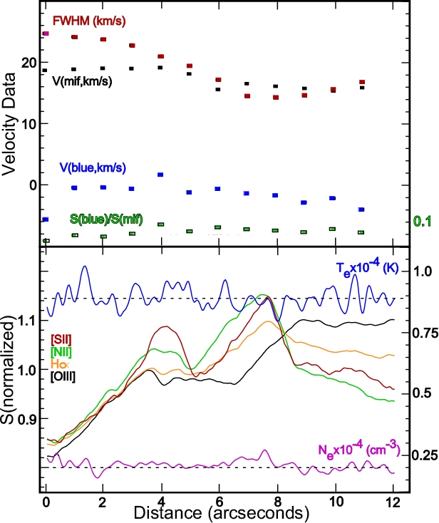
Figure 6: This figure shows the results of a profile across the dark shadow at PA = 195° from $\theta^{1}$ Ori C as shown in Figure 1 and described in Section 4.5. Distance progresses towards PA = 287°. In the upper panel the [N ii] V_r and FWHM information is given using the coordinate values on the left ordinate. The S(blue)/S(mif) values are scaled according to the coordinate values on the right ordinate. In the lower panel the results for the normalized emission-line surface brightnesses are shown, scaled to the coordinate values on the left. In the same lower panel the T_e and n_e values are shown in units of 10⁴ using the right-hand coordinate values.

There are a number of radial features oriented towards $\theta^{1}$ Ori C and models for them predict that their T_e values should be lower than the surrounding gas. We have investigated one of the best defined of these features in order to assess their role in temperature variations across the Huygens Region.

These objects were first noted in both the Huygens Region and NGC 7293 (the Helix Nebula) through images in S([O iii])/S([N ii]) where they appear as a pair of radial lines centred on the ionizing star and being dark in between (O’Dell, 2000). They are essentially shadow cones behind objects that are optically thick to the Lyman Continuum (LyC). The shadowing objects in the Huygens Region are the proplyds. The shadows are only evident if there is ambient material that is photoionized and they can be used to trace the 3-D structure of the nebula (O’Dell, 2009b). Within the shadow cone the ambient gas is illuminated by LyC radiation formed by recombinations of surrounding ionized hydrogen, rather than $\theta^{1}$ Ori C. This radiation field is about an order of magnitude less than that from the star, but is sufficient to cause an ionization front to form on the shadow of the cone. The illuminating LyC photons have a flux distribution more concentrated near the ionization threshold for hydrogen and the photoionized gas on the shadow cone’s surface will have a lower electron temperature. This model created by Cantó et al. (1998) predicts that a profile across a shadow cone will show a low ionization boundary (sharp through limb brightening) with the region between these boundaries be marked by seeing the cone’s ionization front from face on and missing high ionization emission from the ambient gas within the shadow cone.

This is the same process that determines the shape of the tadpole shaped tails of the proplyds (Bally, O’Dell, & McCaughrean 2000). The important difference is that in the case of the proplyds the density of gas in the shadow is determined by the rate of material being lost through photoionization from the side facing $\theta^{1}$ Ori C  and this density decreases with increasing distance from the source. This decreasing density allows the shadowed zone’s ionization front to advance into the centre of the shadow and give the proplyds their characteristic form.

We selected the shadow cone whose centre is at PA = 195° from $\theta^{1}$ Ori C. Figure 1 shows the position of this feature and the sample box taken crossing it. The boundaries cross through the proplyd AC Ori most recently discussed by O’Dell et al. (2015). The sample box was 3$\aas@@fstack{\prime\prime}$5$\times$12$\aas@@fstack{\prime\prime}$0 and oriented towards PA = 287° and the shadow is slightly more than 2$\aas@@fstack{\prime\prime}$0 wide. It was examined both in WFPC2 images in [O iii], [N ii], H$\alpha$, and [S ii] and also in Spectral Atlas [N ii] spectra in steps of 1$\aas@@fstack{\prime\prime}$0.

The results of the profile are shown in Figure 6. The centre of the shadow is at 6$\aas@@fstack{\prime\prime}$2. We see that S([O iii]) increases with distance and dips at the position of the shadow. This is explained as a lack of emission in [O iii] in shadow cone passing through ambient doubly ionized oxygen. The [N ii] background rises as one approaches the shadow from either direction, peaks just inside of the [O iii] dip as one sees the limb brightened ionization boundary on the outside of the shadow, then it dips down as one sees emission from the layer flat-on. The [S ii] profile peaks indistinguishably at the same position as [N ii], which reflects the fact that the shadow’s ionization zone is about 1″ thick. The H$\alpha$ surface brightness illustrates how it arises from all the ionized gas. The radial velocity slowly decreases across the profile and there is only a hint of a local increase at the edges of the shadow’s ionization front, but the spatial resolution of the spectra precludes any interpretation. The same can be said of the large change in the FWHM, although it appears to dip across the shadow. There is only a slow decrease in V_r(Blue) and increase in S(blue)/S(mif) across the shadow, indicating that material affected by the shadow is not part of the Blue Layer.

The backscattered component is not detectable in the first four samples (0″ through 3″), but then begins to be stronger relative to the MIF component, until becoming stronger than in most of our other samples. This absence occurs at positions where the FWHM is high.

The derived n_e increases from the local value of 2000$\pm$200 cm^-3 to about 2300$\pm$200 cm^-3 at the more distant limb brightened [N ii] edge of the shadow. This is interpreted as that edge being of higher density than the ambient more highly ionized gas. There is only a hint of a dip in T_e across the shadow from the local value of 8900$\pm$300 K.

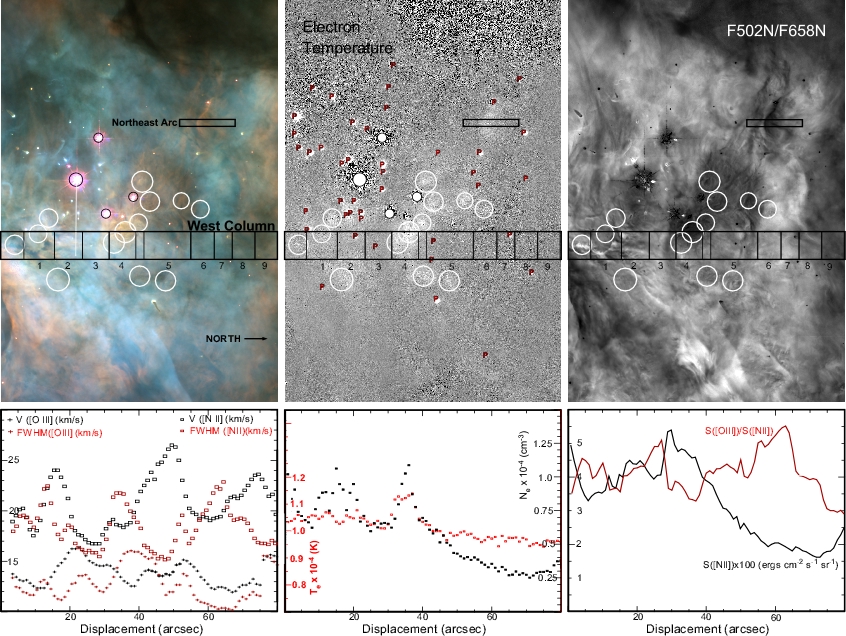
Figure 7: Each top panel shows a 115$\aas@@fstack{\prime\prime}$6$\times$79$\aas@@fstack{\prime\prime}$7 field of view, as shown in Figure 1, except now north is toward the right and east is toward the top. The left top panel is the WFPC2 image as colour coded in Figure 1. The centre top panel is a map of T_e determined from [N ii]. The right top panel shows the ratio of the images of [O iii] (F502N) over [N ii]  (F658N) uncalibrated WFPC2 images. For reference, the sample region for the Northeast Arc, discussed in Section 4.4 is shown in each panel. Each top panel also shows a column of south-north samples as described in Section 4.6. The white circles indicate resolved regions of high T_e and the red ‘P’ letters indicate unresolved high T_e regions associated with proplyds. The lower panels present results for the north-south column in the upper panels taken at 1″ intervals as described in Section 4.6. The numbered groups (1–9) within the West Column are those used in the discussion and in Table 1.

Table 1: Properties of Samples within the West Column

	Group 1	Group 2	Group 3	Group 4	Group 5	Group 6	Group 7	Group 8	Group 9
Range (arcsec)	6–15*	15–23	23–31	32-39	41–54*	55–61	62–66*	67–73*	74–80*
Vr([N ii]) (km s-1)	20.7$\pm$2.6	19.3$\pm$2.5	17.7$\pm$1.0	19.9$\pm$1.7	23.5$\pm$2.4	19.3$\pm$0.1	21.0$\pm$0.7	22.8$\pm$0.8	19.8$\pm$1.9
FWHM([N ii]) (km s-1)	19.5$\pm$1.8	17.0$\pm$1.0	17.7$\pm$2.5	19.6$\pm$1.8	16.7$\pm$1.4	20.8$\pm$1.3	20.2$\pm$1.5	17.8$\pm$0.9	16.4$\pm$0.5
Vr([O iii]) (km s-1)	14.0$\pm$1.0	16.5$\pm$0.6	15.3$\pm$0.3	13.9$\pm$0.5	14.9$\pm$0.5	13.4$\pm$0.5	12.9$\pm$0.2	13.9$\pm$0.9	16.6$\pm$0.7
FWHM([O iii]) (km s-1)	12.9$\pm$0.7	13.4$\pm$0.9	13.6$\pm$0.8	16.5$\pm$0.3	13.6$\pm$1.2	11.3$\pm$0.3	11.2$\pm$0.8	12.9$\pm$1.5	16.5$\pm$1.3
Vr(blue,bluer) (km s-1)	-13.9$\pm$2.7	-6.2$\pm$3.0	-9.6$\pm$1.7	-9.8$\pm$5.6	-8.8$\pm$5.0	-11.4$\pm$3.9	-14.0	—-	—-
Vr(blue,redder) (km s-1)	7.0$\pm$2.3	6.1	—-	3.1$\pm$0.8	9.7$\pm$1.0	—-	1.2$\pm$01.5	4.9$\pm$3.2	0.7$\pm$2.9
S(blue,bluer,[N ii])/S(mif,[N ii])	0.016$\pm$0.003	0.029$\pm$0.006	0.019$\pm$0.010	0.013$\pm$0.005	0.014$\pm$0.003	0.021$\pm$0.006	0.015	—	—-
S(blue,redder,[N ii])/S(mif,[N ii])	0.050$\pm$0.009	0.054	—-	0.058$\pm$0.024	0.117$\pm$0.036	—-	0.049$\pm$0.006	0.076$\pm$0.025	0.044$\pm$0.013
ne(cm-3)	8450$\pm$1250	8360$\pm$1050	6460$\pm$390	8960$\pm$2000	4930$\pm$930	3610$\pm$250	3020$\pm$220	2820$\pm$120	3240$\pm$300
Te(K)	10520$\pm$100	10520$\pm$140	10270$\pm$160	11090$\pm$280	9960$\pm$160	9740$\pm$40	9740$\pm$180	9560$\pm$160	9540$\pm$80
S([N ii])$\times$100 (ergs cm-2 s-1ster-1)	3.62$\pm$0.25	4.29$\pm$0.18	4.50$\pm$0.59	4.54$\pm$0.29	2.92$\pm$0.50	2.03$\pm$0.10	1.88$\pm$0.07	1.70$\pm$0.10	1.99$\pm$0.29
S([O iii])/S([N ii])	3.95$\pm$0.32	4.15$\pm$0.27	4.41$\pm$0.56	3.54$\pm$0.22	4.22$\pm$0.16	5.08$\pm$0.16	5.05$\pm$0.56	3.93$\pm$0.09	3.03$\pm$0.13

*No backscattered red [N ii] component in slits 11″–14″, 41″–50″, 63″–76″.

4.6 Northern Area

The structure of the region near the Trapezium stars is discussed in detail in an earlier publication (O’Dell, 2009b). There it is argued that the appearance of this region is determined not simply by processes occurring near the MIF, but also by a high-ionization shell of gas produced by the stellar wind arising from $\theta^{1}$ Ori C. This shell appears as an incomplete high ionization arc (HIA), being open to the south-west where the Orion-South cloud is located. The inner boundary of the shell corresponds to the boundary of the unimpeded stellar wind with the shocked outer region of that wind. The outer boundary would represent where the outward moving shocked wind gas interacts with the low density ambient gas. O’Dell (2009b) argue that because there is not a surrounding [N ii] boundary (best examined in their wider FOV Figure 3) this shell is not ionization bounded.

The image in Figure 7 includes the north-west through east-southeast portions of the HIA. It appears most clearly as a bright and broad feature in the F502N/F658N (top-right) panel of Figure 7. The low F502N/F658N values in the innermost region and outside of the HIA are interpreted to be due to the dominance of MIF emission. In contrast, the low values to the south-west are due to seeing the north-east boundary of the Orion-South cloud in projection, much like the Bright Bar (O’Dell, 2009b; Mesa-Delgado et al., 2011).

We have prepared a series of eighty samples each 8$\aas@@fstack{\prime\prime}$0 wide and 1$\aas@@fstack{\prime\prime}$0 high along a south to north line centred 19$\aas@@fstack{\prime\prime}$0 west of $\theta^{1}$ Ori C, with the southern limit 21$\aas@@fstack{\prime\prime}$6 south of $\theta^{1}$ Ori C, as shown in each of the top panels of Figure 7. The lower panels present radial velocity and FWHM for the strong [N ii] and [O ii] components determined using ‘splot’ (left panel), our n_e and T_e values (centre panel), and the calibrated S([N ii]) and the S([O iii])/S([N ii]) ratios from calibrated WFPC2 images (right panel). This series of samples begins at the northeast corner of Orion-South, proceeds through the putative centre of the effects of $\theta^{1}$ Ori C’s stellar wind, then crosses the northern boundary of the high ionization incomplete arc. In all of the upper panels the location of known proplyds have been marked by a red letter P and circles indicated the position of resolved high temperature regions not associated with a known proplyd.

In the lower left panel of Figure 7 we see that the the [N ii] velocities are more positive than the [O iii] velocities, which is consistent with the basic model of this region being a photo-evaporating blister with the [O iii] emitting layer having a larger evaporation velocity than the [N ii] emitting layer (Section 3). Beyond this general observation, one must examine all the characteristics at the same place in the West Column. For this reason we have grouped the samples according to their characteristics into a sequence of larger groups and discuss the properties of these groups in the following sections. The numeric results for each group are given in Table 1.

There is a loose correlation (coefficient 0.92) of n_e and S([N ii]) following the relation n_e= -450+1.96$\times\rm 10^{5}\times$ S([N ii]). The former relation indicates the result of the areas of highest surface brightness being those that also experience the highest rate of photo-evaporation of material. Since the S([N ii]) values are not corrected for extinction, the multiplier in this equation would be lower when using extinction-corrected values of S([N ii]).

We see numerous local variations of T_e and explain the cause of the largest in Section 6.2. We see temperature fluctuations of about 400 K across the West Column with size scales of about 5″, with size scales increasing and the magnitude of the temperature fluctuations decreasing as one moves away from the point of the West Column that is closest to $\theta^{1}$ Ori C.

The V_r(blue,[N ii]) values within an individual group often shows a grouping into bluer (about -10.5$\pm$2.8 km s^-1) or redder (about 4.7$\pm$3.2 km s^-1), with the redder component being stronger [S(blue)/S(mif)=0.064$\pm$0.026] than the blue [S(blue)/S(mif)=0.018$\pm$0.006].

4.6.1 The High Ionization Arc Region

Our Groups 6–8 cross the HIA. We see a local enhancement of the S([O iii])/S([N ii]) ratio and the V_r([O iii]) values are lower than the adjacent groups, indicating that the MIF [O iii] emitting zone in these groups is flatter or that there is a negative velocity component of the partial shell that forms the HIA. Given the enhancement of [O iii] emission associated with the HIA, the latter interpretation is more likely to be correct. The jump in V_r([O iii]) and FWHM([O iii]) in Group 9 strengthens this interpretation. The abrupt change in V_r([N ii]) from Group 5 (23.4$\pm$2.0 km s^-1 to Group 6 (19.7$\pm$0.6 km s^-1) and Group 7 (20.0$\pm$1.0 km s^-1) argues that the MIF [N ii] emitting layer has been flattened behind the HIA and has recovered its original orientation by Group 8 (22.4$\pm$0.6 km s^-1) before flattening slightly more by Group 9 (19.7$\pm$1.7 km s^-1). It may be important that no backscattering component can be seen in samples 63″–76″, on the outer boundary of the HIA.

The northern-most samples (Group 9) are expected to be unaffected by the HIA and behave according to the V_rmodel in Section 3 if it is indeed a shocked shell of gas. The low ratio of S([O iii])/S([N ii]) (the lowest in our nine groups) certainly indicates this to be the case. However, Figure 7’s lower left panel shows that FWHM([N ii]) is almost constant while V_r([N ii]) is dropping rapidly. These values for [O iii] are almost equal and show no change across the sample.

4.6.2 The Inner [N ii] Region

The Inner [N ii] Region is a distinctive feature of low ionization found surprisingly close to $\theta^{1}$ Ori C and is most visible in the F502N/F658N image in the top right panel of Figure 7 and it covers 32″ – 54″, with Group 4 well within the region of higher S([N ii]) falling within the HIA and Group 5 being transitional from it to the characteristics of the HIA. It is probably the highest density (mean = 8960$\pm$2000 cm^-3, peak = 11300 cm^-3) and is the highest temperature (mean = 11090$\pm$280 K, peak = 11200 K) of our groups.

In Group 4 V_r(nii) is low (19.9$\pm$1.7 km s^-1) and the FWHM([N ii]) is high (19.6$\pm$1.8 km s^-1) and these reverse in Group 5 (V_r([N ii]) = 23.5$\pm$2.4 km s^-1, FWHM([N ii]) = 16.7$\pm$1.4 km s^-1). This indicates that Group 4 is flatter than Group 5 The V_r([O iii]) and FWHM([O iii]) behave in the same manner (Table 1. However, S([N ii]) is high in Group 4 (where S([O iii])/S([N ii]) is low) and then in Group 5 S([N ii]) has dropped while S([O iii])/S([N ii]) has increased. The V_r and FWHM properties agree with the pattern described in Section 3. The pattern of the surface brightness does not. Within Group 5 most of the samples (41″–50″) have no detectable backscattered component.

It is likely that the low ionization of Group 4 is caused by the lower ionization factor U, the ratio of the flux of ionizing photons to the density of neutral hydrogen (Osterbrock & Ferland, 2006). This is because the flux of ionizing photons is essentially the same in both regions (only somewhat lower in Group 5), but the density is much higher in Group 4.

4.6.3 Properties of the Southernmost Samples of the West Column

Groups 1–3 sample the transition region between the Inner [N ii] Region and the northeast boundary of the Orion-South. When examining their statistics (Table 1) they show little variation, except for the low n_e for Group 3. However, the devil is in the detail as one sees wide fine-scale fluctuations in most of the observed and derived quantities.

Using V_r([N ii]) as a guide, we can trace the changes of tilt across these three groups. The MIF must almost be flat at 25″, then monotonically increases in tilt to a high angle at 14″, then decreases again to the south. There is no detectable backscattering component in samples 11″–14″, which is in the area of decreasing angle of the MIF. The curve of the rise and decay from the 14″ peak is mimicked by a much noisier rise and decrease in n_e. We are probably seeing the effects of a varying flux of ionizing photons in a rapidly rising, then decreasing escarpment in the MIF. This pattern is rendered clearer when considering the range covered within the V_r([N ii]) peaks at 14″ to 47″. The n_e rises occur on the inside side of the two V_r peaks. This argues that there we are seeing a concave pocket in the MIF with a bottom at 25″ and the greatest angles at 14″ and 47″. The continuation of high n_e south of the 14″ velocity peak and not to the north of the 47″ peak indicates that the 14″ peak MIF is physically closer to $\theta^{1}$ Ori C and not just closer in projection on the sky.

5 The Outflows Area

The region shown in Figure 8 contains the sources of many of the large and small-scale stellar outflows in the Huygens Region and has most recently been discussed in detail by O’Dell et al. (2015). The lower-left panel uses the same colour coding as Figure 1. The arrows in all of the images indicate the magnitude and direction of tangential motions (red [N ii] , green [O iii]) using images from HST programs GO 5469 and GO 10921, as described in Section 4.4. The young star COUP 632 is almost certainly the source of the rapidly moving irregular feature HH 1132. COUP 666 lies just north of the FOV and has been drawn as a red filled circle on the upper-left panel, although its coordinate system is that of the lower-left panel. This star is likely to be the source of the narrow feature labeled as the HH 1129-Jet. This feature lies on a projection of a straight line from COUP 666 through a narrow linear feature crossing HH 1132, but passes east of a nearly parallel linear feature labeled as HH 1129. The white line in the lower-left panel show the nominal axis of a series of shocks designated as HH 269. The source of the HH 269 shocks must lie near this line (or its projection eastward) as discussed in O’Dell et al. (2015). The upper left panel illustrates both the motions of objects and also the change in surface brightness of some figures (especially around HH 1129).

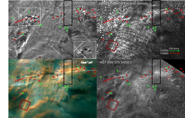
Figure 8: The 32$\aas@@fstack{\prime\prime}$6$\times$21$\aas@@fstack{\prime\prime}$7 panels in this array are all centred on 5:35:12.47 -5:23:58 (2000) as shown in Figure 1. Each panel is described in detail in Section 5. The black rectangle and red square indicate the position of samples discussed in Section 5.1 and Section 5.2.

The upper-right panel gives the results of deriving n_e using the red [S ii] doublet line ratios. The upper left portion of this panel is from the MUSE data set, while the remainder is from HST WFC3 program GO 12543. That program imaged the southwest portion of this FOV with the narrow-band quadrant filters for the [S ii] lines. The quadrant filters are each of slightly less than one-fourth the area of the standard WFC3 filters, but cover more diagnostic lines. The calibration of these filters are described in detail in a study in process by W. J. Henney. The low resolution MUSE n_e maps were carefully merged with the 10 times better resolution WFC3 data. The series of arcs pointing northwest in the lower part of the n_e map are caused by uncorrected filter-fringing and are not important for our discussion.

The lower-right panel shows the ratio of calibrated [N ii] 575.5 nm and [N ii] 658.3 nm emission-lines from the full area GO 12543 WFC3 images. This image is shown (rather than a T_e map because it provides the highest angular resolution and best S/N ratio.

Figure 8 allows one to relate the apparent features to their motions, changes, and conditions. We present here a detailed analysis only for two regions of particular interest. The North Sample is shown as a black rectangle in Figure 8 and is discussed in Section 5.1. The Southeast Sample is shown as a red square in Figure 8 and is discussed in Section 5.2.

5.1 The North Sample West of COUP 632

This region was selected for study because it crosses the axis of the HH 269 flow and many irregular east-west features. The sequence of irregular features about 2″ wide at this point have been designated (O’Dell et al., 2015) as the West-”Jet”. The quotation marks are added here because it is not established that the features represent a collimated flow. The lower part of the feature lies along the nominal axis of the HH 269 flow. The uncertainty of the PA of the axis of the HH 269 flow is about 1°, which corresponds to about $\pm$1″ in declination. The West-”Jet” does not reveal high tangential velocities until its western end. This region is also one of the hottest areas of the Huygens Region. The FOV is 3$\aas@@fstack{\prime\prime}$0$\times$9$\aas@@fstack{\prime\prime}$3 and the [N ii] spectra were taken in samples of 3$\aas@@fstack{\prime\prime}$0 wide by one Spectral Atlas line (0$\aas@@fstack{\prime\prime}$53) high. The calibrated surface brightnesses for [N ii] and [O iii] from the HST images are shown in the right-hand panels of Figure 9.

We have also presented the results of the [S ii] density and uncorrected-T_e profiles in the upper-right panel. Both of these require explanation. The critical density (the density at which it is equally likely that the upper state is depopulated by spontaneous radiative decay or a collisional de-excitation) for the [S ii] doublet lines are about 1000 cm^-3. The critical densities are different for the two upper levels giving rise to the doublet, which make it the useful n_e indicator that it is. However, the low value of the critical densities means that a derived n_e becomes much more sensitive to photometric errors with increasing density and derived densities of more than about 10000 cm^-3 are very uncertain (Osterbrock & Ferland, 2006). We see this in the bright points in Figure 8 and noisy peaks of [S ii] derived values of n_e shown in Figure 9.

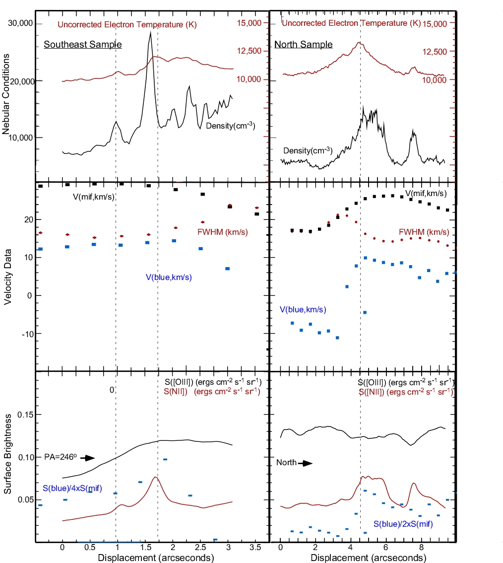
Figure 9: Both the left and right panels of this figure show sets of data as in several preceding figures, but are for the North (black box) and Southeast (red box) samples drawn in Figure 8. These are explained and discussed in Section 5.1 and Section 5.2. The vertical dashed lines are for reference.

The T_e values in this figure are labeled as ”Uncorrected”. This is because they have not been corrected for collisional de-excitation of the upper electron state giving rise to the [N ii] 658.3 nm line. This de-excitation supresses the 658.3 nm line emission and makes the derived T_e value too large. Regions with T_e about 11000 K and density about 5000 cm^-3 will be over-estimated about 3%. The over-estimation increases to 6% at 10000 cm^-3 and 8% at 15000 cm^-3. This means that the peak values of T_e are probably too large by about 1000 K and that the narrow peak in T_e at displacement 7$\aas@@fstack{\prime\prime}$5 can be explained as primarily due to collisional de-excitation. However, this analysis leaves intact that there is a very high T_e (about 12000 K) at displacement 4$\aas@@fstack{\prime\prime}$5.

We see in Figure 9 that n_e and T_e begin and end at about the same values, 3500 cm^-3 and 10450$\pm$150 K, respectively. However, significant increases arise in both, beginning at about 2″. A local peak in T_e occurs at 4$\aas@@fstack{\prime\prime}$5, then it gradually decays to the north, with a local rise at 7$\aas@@fstack{\prime\prime}$5 that is explained above as being due to a local increase in n_e. The electron density essentially peaks at the T_e peak (4$\aas@@fstack{\prime\prime}$5), but is about constant until 6$\aas@@fstack{\prime\prime}$0, before dropping to the background value, interrupted by a strong increase at 7$\aas@@fstack{\prime\prime}$5. The central region (4$\aas@@fstack{\prime\prime}$5 to 6$\aas@@fstack{\prime\prime}$0) of both high n_e and T_e occurs where the samples transit the West-”Jet”. The 7$\aas@@fstack{\prime\prime}$5 n_e peak occurs at an east-west oriented low ionization feature (5:35:14.21 -5:23:48.9, 142-349 in shorthand) that curves northward on its east end.

S([N ii]) rises to a flat peak that agrees in position with the passage of the West-”Jet”, then drops to the background level before peaking at 7$\aas@@fstack{\prime\prime}$5, then returning to the background level. Across the full sample S([O iii]) varies little, except for a small dip from 4$\aas@@fstack{\prime\prime}$0 to 6$\aas@@fstack{\prime\prime}$0, and a sharp and stronger dip at 7$\aas@@fstack{\prime\prime}$3.

This information argues that the West-”Jet” lies within the [O iii] emitting zone near the MIF of the Orion-South cloud that faces the observer. The West-”Jet” is of low ionization, having no emission of its own in [O iii] and excludes only a small amount of [O iii] zone emission. The fact that the 142-349 feature is more than double the local density yet has a surface brightness only one-third higher indicates that this feature is a small fraction of the thickness of the [N ii] emitting layer. We also know that it must be located in the [O iii] emitting zone since that emission dips at the [N ii] bright position. It must be closer to the MIF than the West-”Jet” since it excludes a larger fraction of the [O iii] emission.

V_r([N ii]) is quite low (about 14 km s^-1) at the southern end of our sample, indicating that this region is nearly flat-on. This velocity increases to a broad peak of 22 km s^-1 at 6$\aas@@fstack{\prime\prime}$0, then slowly decreases to 18 km s^-1. This velocity change across the position of the West-”Jet” is certainly broader than that feature. However, when the Spectral Atlas resolution of 2″and the location of the 142-349 feature are considered, the V_r([N ii]) change can be attributed to either the MIF being more tilted there or that the West-”Jet” has a more positive radial velocity. If the West-”Jet” is the driving source of HH 269, then the velocity change is probably due to an increasing tilt of the MIF since the HH 269 shocks are known to be blue-shifted (O’Dell et al., 1992).

The FWHM([N ii]) is nearly constant at about 12 km s^-1, except for a sharp rise that peaks at 18 km s^-1  (peak at 3$\aas@@fstack{\prime\prime}$5, with boundaries at about 2$\aas@@fstack{\prime\prime}$0 to 4$\aas@@fstack{\prime\prime}$5). Examination of Figure 8 shows that this region of unusually large FWHM is where one sees multiple fine-scale tangential motions, indicating small scale motions within the MIF [N ii] emitting zone. The disturbed region runs from 3$\aas@@fstack{\prime\prime}$0 to 5$\aas@@fstack{\prime\prime}$0, indistinguishable from the FWHM anomaly. This region is on the south edge of the West-”Jet” and is probably caused by it.

There is a linear series of low tangential velocity knots east of displacement 4$\aas@@fstack{\prime\prime}$2. They extend from 1$\aas@@fstack{\prime\prime}$0 to 4$\aas@@fstack{\prime\prime}$0 from the east boundary of the North Sample and have PA=275$\pm$2°, indistinguishably the same as the axis of HH 269. This argues that the south border of the West-”Jet”, where T_e peaks, marks the collimated flow that drives HH 269.

Both V_Blue and S(blue)/S(mif) change abruptly from nearly constant values at the lowest displacements to about 17 km s^-1 more positive velocity and five times stronger surface brightness ratio at the same point where the T_e maximum occurs.

The pattern of two preferred blue component velocities at near -10 km s^-1 and +5 km s^-1 has already been seen in the West Column data (Section 4.4) and the Northeast Arc (Section 4.6). Similar to the case with the North Sample, those other regions have the higher radial velocity blue component stronger than the lower velocity counterpart. The higher displacement values of V_Blue are somewhat higher than the characteristic value of 1.8$\pm$1.9 km s^-1. The abrupt changes of the V_Blue component indicate the the Orion-South cloud influences the Blue Layer after the MIF has tilted towards the observer along the northern boundary of the West-”Jet” feature.

5.2 A Newly Identified Feature in the HH 1149-CCW Structure

A fan of shocks emanating immediately to the east of the Orion-South cloud and designated as HH 1149 was recently identified (O’Dell et al., 2015). On its most counter-clockwise (CCW) boundary is an irregular structure designated as HH 1129. At a point immediately north of the red box in Figure 8 HH 1129 changes PA by a few degrees CCW and retains its broad structure. There is a newly discovered feature, which we call the HH 1129-Jet, which parallels HH 1129 and lies exactly on a line projecting back along the northern parts of HH 1129, through the jet feature 149.1-350.2 that crosses HH 1132, and then reaches COUP 666 (Section 5). These two features are quite different, with the HH 1129-Jet being straight, narrower, and of lower ionization.

We show a sample that includes both the HH 1129 extension and the HH 1129-Jet in Figure 10. This sample was divided along lines pointing toward PA = 336° (parallel to the two targeted features) with sample spacing of the spectra of 0$\aas@@fstack{\prime\prime}$5. The resulting profiles (increasing distance from the eastern edge of the sample) are shown in the left-hand panels of Figure 9.

Scanning with increasing displacement we see that there are density peaks associated with the passage of the the HH 1129-Jet (1$\aas@@fstack{\prime\prime}$0) and HH 1129 (1$\aas@@fstack{\prime\prime}$7. Much, but not all of the T_e increase at 1$\aas@@fstack{\prime\prime}$0 and 1$\aas@@fstack{\prime\prime}$7 can be attributed to the local rise of T_e. The spatial resolution of the spectra preclude drawing detailed conclusions from them. However, it is clear that V_r([N ii]) drops upon entering the region to the west and the FWHM([N ii]) increases. Values of V_Blue drop after reaching the HH 1129 boundary.

The low displacement spectra are interesting in that the V_r values of about 29 km s^-1 are larger than the assumed velocity (27.4$\pm$1.5 km s^-1) of the Orion Molecular Cloud (Section 3. This argues that the radial velocity of the PDR does change slightly across the Huygens Region or that this particular region (east of our sample) has a collective motion into the host molecular cloud. The spectra are also unusual in that the S(blue)/S(mif) values are much stronger than elsewhere (the next highest is 0.18 in the Secondary Bright Bar) reaching a peak of 0.38, then dropping to being too faint to detect. As in other sections, the blue component velocities are stronger when the velocity is more positive. In addition, there is no detectable backscattered redshifted component for any of these samples. This is consistent with the idea that we should not expect to see a backscattered component when viewing a region tilted edge-on.

The radial velocity changes indicate that one progresses from a highly tilted region into a MIF that is flatter, with the increase of local n_e and T_e occurring at the position of this transition. The HH 1129-Jet is of higher density than the MIF in that direction and probably much higher since the object is intrinsically small. There is no dip in S([O iii]) at its position, indicating that it is not in a strongly emitting [O iii] zone.

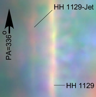
Figure 10: This 3$\aas@@fstack{\prime\prime}$20$\times$3$\aas@@fstack{\prime\prime}$24 image is of the SE Sample outlined in red in Figure 8. The colour coding is the same as in the previous colour images, but the colour balance has been changed for clarity.

6 Discussion

The wealth of information derived in the subsections of Section 4 has allowed us to examine multiple facets of the structure and physics of the Huygens Region. The first is the unexplained line broadening found in high velocity resolution studies of the Huygens Region (Section 6.1). Next we were able to establish that the variations of T_e are determined by variations in n_e, down to a scale of a few arcseconds (Section 6.2). Finally, we determined that the lack of a red-shifted back scattered component is due to viewing highly tilted regions of the MIF (Section 6.3).

6.1 Unexpected large values of the FWHM

It has been recognized for several decades that the FWHM of lines in the Huygens Region are unexpectedly high. This was initially recognized in the photographic study of Wilson et al. (1959) and was interpreted by Münch (1958) as fine-scale turbulence. Typically this unexplained component is equal to or larger than the thermal broadening of the lines, which means that we are not able to explain a large amount of energy carried in the lines. We address this problem in this section, first summarizing earlier studies (Section 6.1.1, then presenting and testing a simple model for explaining the extra broadening (Section 6.1.2). Finally (Section 6.1.3) we summarize the results of the discovery study and discuss their relevance today.

6.1.1 Previous studies of the unexplained component of the FWHM

A slab of ionized gas will produce emission-lines of a finite FWHM. In the simplest case, the observed FWHM will be the quadratic sum of the thermal broadening component (5.44 km s^-1 for [N ii] at 9000 K) and the instrumental broadening component (typically 8 to 10 km s^-1). If there is an additional broadening mechanism that is random, it too will add quadratically; but, if it is small and systematic, it will add arithmetically. Here we will designate the additional components as the ’Extra Line-Broadening Component’ (ELBC).

The highest spectral resolution study of the ELBC is that of O’Dell et al. (2003) , where spectra at 6 km s^-1 resolution were used to study a group of 10 slit spectra, nine of which were inside the Bright Bar and one outside. They found the quadratically extracted extra component for multiple emission lines: [N ii]  658.3 nm, 10.6$\pm$1.4 km s^-1; H$\alpha$, 20.9$\pm$1.3 km s^-1; H$\beta$, 18.8$\pm$2.2 km s^-1; He⁺, 587.6 nm, 18.4$\pm$1.9 km s^-1; [O i], 630.0 nm 9.0$\pm$2.1 km s^-1; [O iii], 500.7 nm, 13.0$\pm$3.7 km s^-1; [O iii], 495.9 nm, 11.3$\pm$2.1 km s^-1; [S ii], 673.1 nm, 11.3$\pm$2.4 km s^-1; [S iii], 631.2 nm, 11.8$\pm$1.9 km s^-1. They also report the radio H65$\alpha$ value of 19.6$\pm$0.9 km s^-1(Wilson et al., 1997), and Jone’s (1992) value for [O ii] of 10.5$\pm$2.5 km s^-1. García-Díaz et al. (2008) demonstrated that the H$\alpha$ and H$\beta$ lines need to be corrected for fine-structure. After correction for this, ELBC(H$\alpha$) = 19.5 km s^-1 and ELBC(H$\beta$) = 18.0 km s^-1.

The quadratically extracted ELBC values can be compared and grouped according to the common regions of origin and their dependence on T_e: Group 1 ([S ii], [N ii], [O ii], [S iii]) has an average of 11.1$\pm$0.6 km s^-1; Group 2 ([O iii]) 12.2$\pm$2.5 km s^-1, and Group 3 (H$\alpha$, H$\beta$) 18.6$\pm$0.9 km s^-1). The H65$\alpha$ value was not included in Group 3 because the large beam width of the radio observations means that large-scale motions must contribute to the observed FWHM. The [O i] emission (ELBC = 9.0$\pm$2.1 km s^-1) does not fall into any of these groupings since it arises immediately at the MIF. Group 1 originates in the He^o+H⁺, Group 2 in the He⁺+H⁺, and Group 3 in both the He^o+H⁺ and the He⁺+H⁺ and its emissivity rises with lower T_e, while the emissivity in the collisionally excited forbidden lines increases with T_e.

O’Dell et al. (2003) pursued an explanation that the ELBC in hydrogen (they included the similar numbers for He⁺) and the other ions was due to the fact that the recombination lines (hydrogen and helium) arise from the cool gas along the line-of-sight, whereas the collisionally excited forbidden lines arose in the hot component. When grouped according to the zones of emission, this interpretation continues to make sense because the Group 1 and Group 2 values are very similar, 11.1$\pm$0.6 km s^-1and 12.2$\pm$2.5 km s^-1 respectively, with only Group 3 being different (18.6$\pm$1.5 km s^-1).

We should note that García-Díaz et al. (2008) analyzed the widths of many lines in the Spectral Atlas by an alternative line profile fitting method and a corresponding statistical treatment. Their values of the FWHM yield ELBC components a few km s^-1  greater in value and somewhat greater uncertainty for the forbidden lines (14.3$\pm$3.9 km s^-1) than in the O’Dell et al. (2003) study (11.2$\pm$2.3 km s^-1). Their ELBC for H$\alpha$ is 18.6$\pm$5.1 km s^-1, compared with our Group 3 value of 18.6$\pm$1.5 km s^-1. Through a detailed argument used in deriving T_e from the FWHM values for several ions, they conclude that there is no difference between the ELBC for collisionally excited and recombination lines. The complexity of their approach creates some uncertainty in this conclusion and we will consider in our discussion both possibilities, i.e. that the ELBC for cool and hot gas is the same or different . In any event, the ELBC as measured by collisionally excited lines is indistinguishably the same in the two ionization zones present in the Huygens Region.

The advantage of our study is that we have considered separately the results from many samples for the [N ii] 658.3 nm using the Spectral Atlas. Although (García-Díaz et al., 2008) states that the instrumental resolution is 10 km s^-1, the data is from several sources with a range of resolutions. The spectra of Doi et al. (2004), have a resolution of 8 km s^-1 and were used for the [N ii] and [O iii] lines employed in this study. It is possible that the resolution was degraded as the original spectra were cast into the convenient form of the Spectral Atlas. For this analysis we adopt 10 km s^-1.

In addition to V_r, the determination of the FWHM is an integral product of using the task ”splot”. When a line gave even a hint of being multiple (through an unusually high value of FWHM or an asymmetry of the line profile, an attempt was made to fit multiple components. This was only necessary on rare occasions. The accuracy of V_r is usually better than 1 km s^-1 and the determination of FWHM was usually better than 2 km s^-1.

6.1.2 A role of photo-evaporative flow in determining the FWHM?

Figure 11: This figure compares the observed values of V_r([N ii]) and FWHM([N ii]) with the predictions of the simple model presented in Section 6.1.2 where the extra broadening is due to photo-evaporative flow. The lower line is the expected relation if there is no effect of photo-evaporative flow, the second line applies if the component is added quadratically, and the upper is the expected relation if photo-evaporative flow is linearly added to the FWHM. The numbered samples are those from the West Column (Section 4.6), Sh is for the Shadow Sample (Section 4.5), N for the North Sample (Section 5.1), SE for the Southeast Sample (Section 5.2), HH for the HH 204 Sample (Section 4.1), NE for the Northeast Arc (Section 4.4), BB for the Bright Bar (Section 4.2), and SecB for the Secondary Bright Bar Sample (Section 4.3).

The overall blue-shifting of lines from different stages of increasing ionization gave rise to the widely accepted blister model of the Huygens Region and in this paper we have established that the local variations in V_r can be explained by variations in the tilt of the ionization front. Evaporative expansion certainly occurs and it has previously been argued from models of the photo-evaporative flow that it cannot account for the ELBC (Henney, 2005a). Never-the-less, we found it useful to test that conclusion using both FWHM([N ii]) and V_r([N ii]) data together in a comparison with a simple model.

There are two ways of possibly adding the effects of photo-evaporating flow to what we observe. The results of these two approaches are shown in Figure 11. If the FWHM is determined by quadratic addition of the thermal (5.44 km s^-1 for T_e= 9000 K) and instrumental broadening (10 km s^-1), then the expected FWHM would be constant at 11.4 km s^-1. The photo-evaporating flow accelerates from the velocity of the underlying PDR towards the observer reaching a velocity of about 10 km s^-1 averaged over the [N ii] emitting layer. When one views the MIF where it is tilted edge-on, the photo-evaporating flow will not contribute to the FWHM and the observed V_r([N ii]) will be that of the PDR. This would be a single value of V_r([N ii]) =27.4 and FWHM([N ii]) = 11.4. In the case when one views the MIF flat-on, one expects V_r([N ii])= 17.4 km s^-1 and the FWHM will be increased because of the range of velocities within the [N ii] emitting layer. If this component added quadratically, the FWHM at V_r([N ii])= 17.4 km s^-1 would increase to 15.2 km s^-1. However, this broadening component is systematic, rather than random, and an arithmetic addition is a more accurate description. In this case the value at V_r([N ii])= 17.4 km s^-1 would be 21.4 km s^-1, although such an extreme result is unrealistic because in that case the method of using "splot" would identify such a line as double, rather than producing a wide single-line component. This means that the upper line in Figure 11 is unrealistically high.

The only certain conclusion that can be drawn from Figure 11 is that all of the data points fall on the same plane! Although photo-evaporative flow must play a role in producing the non-thermal line broadening, it can only be inferred for the points lying well beneath the upper line. The effect must be present, but is not established from this data-set. Certainly the points lying above the upper line are not produced in this way. This would be true even if one used the [O iii] expansion velocity (which would certainly apply to the ionized hydrogen emission) of 15 km s^-1.

These conclusions mean that although photo-evaporation must play a role in producing the anomalous FWHM, there remains an unexplained major contributor. The study of O’Dell et al. (2003) remains an important guide and if the ELBC for ionized hydrogen is much larger than for the collisionally excited ions, then line-of-sight variations in T_e is the important factor, rather than turbulence. However, if there is not a systematic difference in the ELBC then turbulence is probably the source. In fact, the simulations of a photo-evaporative gas by Mellama et al. (2006) show that this can be generated by flows off of dense knots within the PDR.

6.1.3 Comparison of the results of this study with an earlier velocity study of the Huygens Region

In a classic study of the Huygens Region  Wilson et al. (1959) mapped the face of the nebula with multi-slit spectra in multiple emission lines. This work and the conclusions that could be drawn were summarized in Münch (1958). The velocity and angular resolution was comparable to that in the Spectral Atlas. The detector was the photographic emulsion and the difficulty of obtaining photometric results caused the authors to simply study the radial velocities and FWHM. Figure 4 of Münch (1958) shows the velocity results for an east-west sample and this resembles the nearby data presented in our Figure 7, which is of a north-south sample.

However, their interpretation of the velocity variations as being large-scale random turbulent motions is probably incorrect. The adopted model of the nebula was an ionized gas whose dust component renders it optically thick to its own emission, making it appear to be a flat surface-which had been treated in the recent theoretical papers on turbulence. Subsequently, there were several similar studies done by the lead author and his students based on the blister model (c. f. Section 3.4.2 of O’Dell (2001)), interpreting the velocity variations within the paradigm of large-scale turbulence. We now know that the variations in velocity are primarily caused by the photo-evaporating ionization front being viewed from different angles along the line of sight. Moreover, recent theoretical work (Medina et al., 2014) shows that one cannot interpret the variations as turbulence. Never-the-less, Münch (1958) correctly identified the source of the non-thermal FWHM as being due to turbulence.

6.2 A Summary of T_e and n_e variations and their causes

The study of many samples throughout the Huygens Region has given us a good idea of the magnitude of the n_e and T_e variations, the relation of these two quantities, and their spatial scale. In this section we describe the relation of n_e and T_e , compare this relation with predictions of the best model for the Huygens Region, then describe the contributing factors to the n_e variations.

6.2.1 Systematic Changes in n_e and T_e

Examination of the n_e and T_e values in the nine groups within the West Column as presented in Table 1 indicated a correlation between these two properties and we have extended this data-set by determining these values at the peak and backgrounds for the other samples. The ten additional results are given in Table 2. In this case we cannot accurately determine the uncertainty of each entry because we are picking points from a graph, whereas for the West Column samples the uncertainty is derived from the spread of values within the group. All of these results are summarized in Figure 12.

Table 2: Observed n_e and T_e values

Region	Background	Peak	Observed	Observed
	ne (cm-3)	ne (cm-3)	Background Te (K)	Peak Te (K)
HH 204	1000	5000	8000	9300
Bright Bar	1800	3400	8750	9100
Sec.Brt.Bar	2700	4700	9200	9800
Shadow	2850	—-	8900	—-
NorthSample	5500	—-	10500	—-
NE Arc	3000	6500	9700	10900

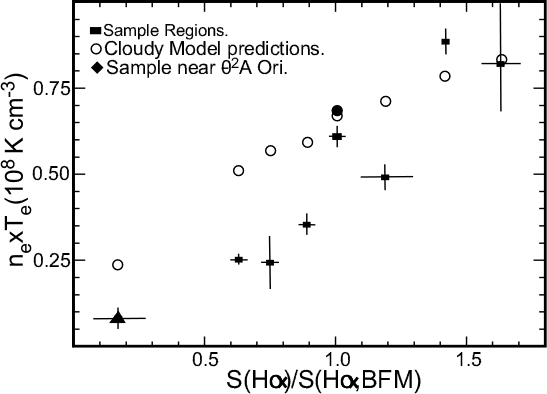
Figure 12: The n_e$\times$T_e values using data in Table 1 and Table 2 were grouped into samples of similar S(H$\alpha$) and are shown as filled rectangles, with the S(H$\alpha$) values taken from the MUSE extinction corrected image. The S(H$\alpha$) values are normalized to the reference sample of Baldwin et al. (1991) (BFM). Sample 5 is from Table 1 and the open rectangle is for the Bright Bar. The reason for their horizontal error-bar arrows are discussed in the text. The lower-left filled triangle is a sample beyond the Bright Bar that is probably partially photoionized by $\theta^{2}$ Ori A. The open circles are the results of models similar to that in BFM as described in the text. The filled circle gives the n_e$\times$T_e value calculated from the line ratios in BFM.

6.2.2 The predicted relation of n_e$\times$T_e and S(H$\alpha$)

The observations presented in Figure 12 demonstrate a correlation between S(H$\alpha$) and n_e$\times$T_e. The former quantity is proportional to the flux of ionizing photons and the latter quantity is proportional to the gas pressure near the MIF as derived from [S ii] and [N ii] emission lines. A correlation of these quantities is expected for a blister model of an Hii region in equilibrium.

In such a model, the geometry consists of an inner bubble of very hot (T about 10⁷ K) stellar-wind-shocked gas, with the Hii forming a boundary between this bubble and the surrounding molecular cloud. The Hii region pressure is established by the combination of radiation pressure in the absorbed stellar radiation field, which often dominates, and the pressure in the inner hot bubble.

Predictions of the best extant model for the Huygens Region are also shown in Figure 12. These Cloudy models were built upon the successful BFM model of an inner region of the nebula using the Cloudy package (Ferland et al., 2013). We assumed that S(H$\alpha$) indicates the conditions at the illuminated face of the Hii region. We took S(H$\alpha$) at each position as an initial condition and then computed a model in which all the forces are in balance.This tests the hypothesis that radiation pressure sets the density.

The predicted values of n_e$\times$T_e and S(H$\alpha$) agree with the observations in the brightest part of the nebula (except for Sample 5 which is discussed in the following section). However, at lower surface brightnesses the observed n_e$\times$T_e is lower than predicted.

6.2.3 Comparison of the Observed and Predicted values of n_e$\times$T_e

The observed points in Figure 12 are subject to systematic effects. When the local samples are highly tilted the n_e$\times$T_e  values will be unchanged since this depends upon the ratio of lines within a narrow ionization zone. However, S(H$\alpha$) will be enhanced due to the projection effect along the tilted MIF. We see this effect most dramatically in the Bright Bar sample, which is known to be highly tilted and in Sample 5, where V_r reaches 26.8 km s^-1 indicating a highly tilted region. The amount of the overestimate of S(H$\alpha$) is uncertain, but would be two times in the case of a tilt of 60°. This means that the Bright Bar and Sample 5 values of S(H$\alpha$) must be corrected by an unknown but large amount to lower values.

The fact that the lower S(H$\alpha$) values systematically lie lower than the predictions of the models can be explained by the fact that the ratio of radiation pressure at the MIF and the hot core gas has been assumed constant. However, this need not be the case as the radiation pressure will drop inversely as the square of the distance from $\theta^{1}$ Ori C and the hot core pressure will decrease more slowly.

Our models have not included any pressure term for turbulent pressure, that is, the random motion of packets of gas. Inclusion of such a pressure term would drop the predicted value of n_e$\times$T_e  by an amount depending upon the density and turbulent velocity. If this is the cause of the disagreement in the low S(H$\alpha$) samples, then this indicates that turbulence becomes relatively more important there. One of the important conclusions of this paper is the confirmation of the conclusions of O’Dell et al. (2003) that there is fine-scale structure at the MIF. The local flow off of these volume elements will simulate turbulence.

6.2.4 The multiple features that produce variations in n_e

One component of the variations in n_e are variations in densities within the PDR, which in turn reflect variations in density of the nearby molecular cloud. Photo-evaporation of gas from the PDR is a very dynamic process, with material being removed. The ionization front will advance into the molecular cloud in those regions of lowest density, thus isolating the higher density knots. On a large-scale this is probably what produces the structured surface of the ionized layer, with the most extreme example being the dense Orion-South cloud. In the case of the Orion-South cloud the ionization front has eaten its way behind the cloud, so that we see in optical wavelengths radiation from the near side of the cloud and at radio wavelengths emission from both the f front and rear. Molecular and 21-cm absorption lines indicate that the Orion-South cloud has a neutral molecular core (O’Dell & Harris, 2010; van der Werf et al., 2013). A second component of the variations arises from when the MIF is tilted to face $\theta^{1}$ Ori C, the flux of ionizing photons increases and the rate of photo-evaporation increases, producing a local rise in density. We see this in the tilted features like the Bright Bar having higher n_e values than the local region.

The hypothesis of there being significant density variations in the PDR and host cloud is also supported by the fact that the radial velocity changes across the nebula. The clearest example is in the West Column samples, where V_r([N ii]) changes significantly over size scales of 10″ or less. Since these variations are caused by varying tilts in the ionization front, the velocity variations mimic the fine-scale structure. There is corroborating evidence for clumpy structure behind the PDR in the high resolution radio studies of molecules in the Bright Bar (van der Werf et al., 1996).

The result that there are variations of n_e and T_e down to the limits of resolution of this study may have a role in explaining the Abundance Discrepancy Factor (ADF), the fact that one derives different relative abundances for heavy elements when using recombination or collisionally excited forbidden lines (Peimbert, 1967, 1969; Mesa-Delgado et al., 2008). The ADF was not resolved by proposing the existence of a non-thermalized electron energy distribution (commonly called a Kappa distribution) as shown in Ferland et al. (2016). It is most likely that the explanation lies in the small scale n_e and T_e variations that also give rise to the turbulence component of the line broadening.

This study has mapped the T_e variations in two dimensions, with single samples being an integral along those lines-of-sight. If small-scale density structures exist, then those structures will have their T_e increased because of suppression of forbidden-line heating, but also through increased dissipation of turbulence and shocks.

In this study we have been limited by the sample size necessary to obtain a high S/N ratio. A more discriminating study would require a spectrophotometric map at HST imaging resolution, accompanied by matching high velocity resolution spectroscopy. The former goal is being pursued by W. J. Henney.

6.3 Samples without a Backscattered Component

A red component in the [N ii] emission-line is present in almost all of our samples. This is to be expected within the paradigm that it is backscattering from dust in the underlying PDR. Within this model, one would expect it to be most visible in sections of the MIF seen face-on and to be weak or absent in those seen edge-on. This means that the fact that it is absent must be telling us about the local conditions.

It is absent in all slits of the SE sample. The V_r is about 29 km s^-1 in the lower displacements and 22 km s^-1 in the higher. The appearance of image of this region is that of an open separation between two volumes, with the HH 1129-Jet passing between. The high V_r of the smaller displacements indicates a highly tilted region and the lack of backscattering is to be expected. The absence at higher displacements is puzzling, but this is an admittedly complex region.

Backscattering is absent in slits 1–4 of the Shadow, where V_r is higher (19 km s^-1), than the remaining region (15.5 km s^-1). Emission from the edge of a low ionization column within the He⁺+H⁺ layer should not have backscattering, which is probably the interpretation of this object.

There is no backscattering in the Secondary Bright Bar spectra. It is a situation similar to that of the SE sample, where one side is very high V_r (27 km s^-1) , hence highly tilted. However, we again have a situation where the nearby regions of lower velocity (21 km s^-1) share the lack of a backscattered component.

In the West Column samples the red component is absent at lines 11–14, 41–50, and 63–76. These appear at displacements about 2$\aas@@fstack{\prime\prime}$5 greater than the line numbers. These coincide with the three V_r maxima in the West Column (24 km s^-1, 27 km s^-1 and 24 km s^-1).

Except for the low displacement Shadow samples (where there is an alternate explanation), all of the samples without backscattering are associated with a highly tilted region of the MIF. At the same time, there are no high velocity samples that do have backscattering, thus strengthening the conclusion that backscattering arises from the PDR and is not seen when the PDR is highly tilted.

7 Conclusions

The variations of radial velocity of the MIF components can be explained as viewing a photo-evaporating ionization front from various angles relative to the line-of-sight.

T_e and n_e variations are common across the Huygens Region, and there is a patten of n_e$\times$T_e  varying with the local surface brightness in H$\alpha$. Comparison with models of the ionized layer indicates good agreement for the high surface brightness samples. The systematic differences in the low surface brightness samples indicates that the assumptions of the model must not be exact there.

There is a blue shifted spectral component in almost all of the regions studied and this often varies in velocity and strength in the same places that the MIF velocities vary.

The absence of a red shifted backscattered component is well associated with regions of high V_r that must be regions viewed more edge-on.

All of the samples show FWHM higher than expected from thermal and instrumental broadening. Large-scale photo-evaporative flow must contribute at some level, but certainly cannot explain this excess. It is necessary to invoke a broadening component originating from fine-scale knots present at the ionization front and into the [N ii] emitting zone. Photo-evaporation from these knots probably drive turbulence in the ionized gas.

An attempt to determine T_e for H⁺ from combined radio and optical observations showed a general agreement with T_e([N ii]), but more important, that the wavelength dependence of the extinction transitions from the more grey extinction in the Huygens Region to the colour dependence of the general interstellar medium at the position of the Bright Bar.

Appendix A An attempt to determine T_e for H⁺ yields information about the extinction curve

The common assumption in determining relative abundances is that the T_e found from forbidden lines also applies to the coexisting H⁺. If this is not true, it will affect the derived relative abundances. In the following section we describe previous methods used to independently derive the T_e that applies to H⁺ and in the following sections describe an attempt using a new method.

A.1 Earlier Methods for Determining T_e for H⁺

In a pure hydrogen gas one can derive the electron temperature of H⁺ from the relative strength of the H$\beta$ line to the underlying continuum (AGN3), but in the case of the Huygens Region, there is a strong stellar scattered light component that is much stronger than the nebular emission (Baldwin et al., 1991; O’Dell & Harris, 2010). This dominant contaminating component prevents one from determining accurate values of T_e by the optical line-continuum ratio method.

T_e can also be determined from the ratio of surface brightness in hydrogen radio recombination lines and the underlying continuum (which has no stellar scattered light component). The studies by Wilson et al. (1997) and Wilson, Bania $\&$ Balser (2015), illustrate the power of this method, but the state of the art is that the angular resolution is about 2$\aas@@fstack{\prime}$5  which covers the Huygens Region. For reference the distance between the brightest star in the Trapezium ($\theta^{1}$ Ori C) and $\theta^{2}$ Ori A (which lies to the southeast and just beyond the Bright Bar feature) is 2$\aas@@fstack{\prime}$24. The Wilson et al. (2015) study found T_e = 8300$\pm$200 K, which is consistent, after consideration of their lower spatial resolution, with the T_e values that we find.

A.2 A new method for determining T_e using radio continuum and optical lines

Comparison of the surface brightness of the nebula in the radio continuum with a Balmer emission line can be used to determine the extinction. This was first explored by O’Dell & Yusef-Zadeh (2000). They used Very Large Array (VLA) observations of the free-free continuum of H⁺  and an assumed constant T_e to predict the surface brightness in the Balmer H$\alpha$ line. The ratio of the observed and predicted H$\alpha$ surface brightness (S(H$\alpha$)) gave an indication of the amount of extinction, expressed as c_Hβ(the logarithmic extinction at H$\beta$), defined as c_Hβ = log (S(H$\rm\beta,OBS$)/S(H$\beta$,Predicted). This result is dependent upon the assumed T_e.

The more common method of establishing the amount of extinction is from measurement of the observed H$\alpha$/Hb ratio and interpreting the difference from an assumed intrinsic value as due interstellar reddening, for example Weilbacher et al. (2015). The assumed intrinsic line ratio is dependent on the assumed T_e.

Since both of these two methods assume a value of T_e, it is possible to eliminate c_Hβ as a variable and derive T_e for the H⁺ emission.

A.2.1 Derivation of c_Hβ from radio and optical observations

In their study of the extinction O’Dell & Yusef-Zadeh (2000) employed observations made with the Very Large Array (VLA) together with calibrated images of the Huygens Region made with the Hubble Space Telescope (HST). The VLA observations of the continuum were made at 20.46 cm wavelength and have a FWHM resolution of 1$\aas@@fstack{\prime\prime}$83 by 1$\aas@@fstack{\prime\prime}$65, with the long axis pointed towards PA=-34 °. This image was converted to units of ergs s^-1 cm^-2 sr^-1. Because the HST images were more than an order of magnitude higher resolution, they were degraded using the IRAF task “gauss” to match the VLA image. The VLA image was used to predict the expected surface brightness in the H$\alpha$ line. A comparison of the observed and predicted surface brightness and the assumption of the form of the extinction law allowed the derivation of c_Hβ at this resolution across the Huygens Region. They then qualitatively compared the resulting map of c_Hβ with that derived from the S(H$\rm\alpha,OBS$)/S(H$\rm\beta,OBS$) ratio over a small portion of the Huygens Region. In a later paper (O’Dell, 2009b) these results were discussed further and it was shown in their §2.4 that the interpretation of the extinctions derived by the two methods was more complex.

In the present study we employ the earlier VLA observations, but utilize the S(H$\rm\beta,OBS$) images derived at about 1″ resolution (sampled at 0$\aas@@fstack{\prime\prime}$2) during the commissioning of the MUSE spectrograph (Weilbacher et al., 2015). For the remainder of this paper we will designate as c_VLA the c_Hβ value derived from a combination of VLA and S(H$\rm\beta,OBS$) and the c_Hβ value derived from the S(H$\rm\alpha,OBS$)/S(H$\rm\beta,OBS$) ratio as c_MUSE.

O’Dell & Yusef-Zadeh (2000) describe the methodology of deriving c_Hβ using the VLA image using the formulation in an earlier version of AGN3. Our approach is the same, but we express the mathematical relations using S(H$\rm\beta,OBS$) in ergs s^-1 cm^-2 sr^-1rather than photons s^-1 cm^-2 sr^-1. More important is that we now include the role of variations in T_e, which was assumed to be constant (9200 K) by O’Dell & Yusef-Zadeh (2000).

The surface brightness in the radio continuum will be

$$\rm I_{\nu}=\frac{2kT_{e}}{\lambda^{2}}(1-e^{-\tau_{\nu}})$$ (1)

ergs cm^-2 s^-1 hz^-1 ster^-1, where k is Boltzmann’s constant, $\lambda$ the wavelength, and $\tau_{\nu}$ the optical depth in the radio continuum through free-free processes at $\lambda$. S(H$\beta$) will be

$$\rm S_{H\beta}=\frac{3.086x10^{18}}{4\pi}\alpha^{eff}_{H\beta}E_{H\beta}EM$$ (2)

ergs cm^-2 s^-1 ster^-1, where $\rm\alpha^{eff}_{H\beta}$ is the emissivity of H⁺, $\rm E_{H\beta}$ is the energy in an H$\beta$ photon, and EM is the commonly used term “Emission Measure” (the integral of n_e$\times$N(H⁺) along the line of sight) in units of cm^-6pc. n_e  and N(H⁺) are the densities (cm^-3) of electrons and ionized hydrogen respectively.

$\tau_{\nu}$ is also proportional to EM. AGN3 gives

$$\rm\tau_{\nu}=0.0824T\rm_{e}^{-1.35}\nu^{-2.1}_{ghz}EM.$$ (3)

There will also be an absorption component from singly ionized helium (the highest state of ionization of helium found in the Huygens Region), so that $\tau_{\nu}$ is increased by about 10$\%$.

Introducing the common notation that t = T_e/10000 and combining equations 1, 2, and 3 gives

$$\rm c_{VLA}=log~{}\Bigl{\{}\frac{t^{1.35}f_{eff}[-~{}ln(1-I_{\nu}/t\times 6.596\times 10^{-15})]}{5.32\times S(\rm H\beta,OBS)}\Bigr{\}}$$ (4)

where f_eff is the electron temperature dependent scaling factor for $\alpha^{eff}_{H\beta}$. Using the values in Table 4.2 of AGN3, we find f_eff = t^-0.83. The resulting c_Hβ map of the Huygens Region for T_e 9200 K is very similar to Figure 2 of O’Dell & Yusef-Zadeh (2000)

A.2.2 Derivation of c_Hβ from the S(H$\rm\alpha,OBS$) to S(H$\rm\beta,OBS$) ratio

The derivation of c_MUSE is less involved as it involves only S(H$\rm\alpha,OBS$) and S(H$\beta$,OBS). It is calculated from

$$\rm c_{MUSE}=\frac{1}{\bf{r}}\Bigl{\{}log\frac{S(H\alpha,OBS)}{S(H\beta,OBS)}-log\Bigl{[}\frac{S(H\alpha)}{S(H\beta)}\Bigr{]}_{t=1}-log~{}g(t)\Bigr{\}}$$ (5)

where [S(H$\alpha$)/ S(H$\beta$)]_t=1 is the line ratio at T_e= 10000 (2.87 from AGN3) and g(t) is a function of the electron temperature and is approximately g(t)=t^-0.086 (again using the numbers in Table 4.2 of AGN3).

The greatest uncertainty in this derivation is in the wavelength dependent extinction factor. It is well known that the Orion reddening curve is much flatter (more like grey extinction) than that for the general interstellar medium (ISM). The most thorough investigation is that of Blagrave et al. (2007) where the shape of the Orion Extinction Curve was derived most accurately. They express the Extinction Curve, f_λ, normalized to zero at the wavelength of H$\beta$. In their nomenclature r = f${}_{486.1\ nm}$-f${}_{656.3\ nm}$, which is 0.22 as calculated from their Table 2. r would be much larger using the Extinction Curve from the ISM and would be smaller for even more grey extinction. Our derived c_MUSE map is very similar to that of Weilbacher et al. (2015), where they assumed an intrinsic and flux ratio of 2.89 of H$\alpha$ and H$\beta$.

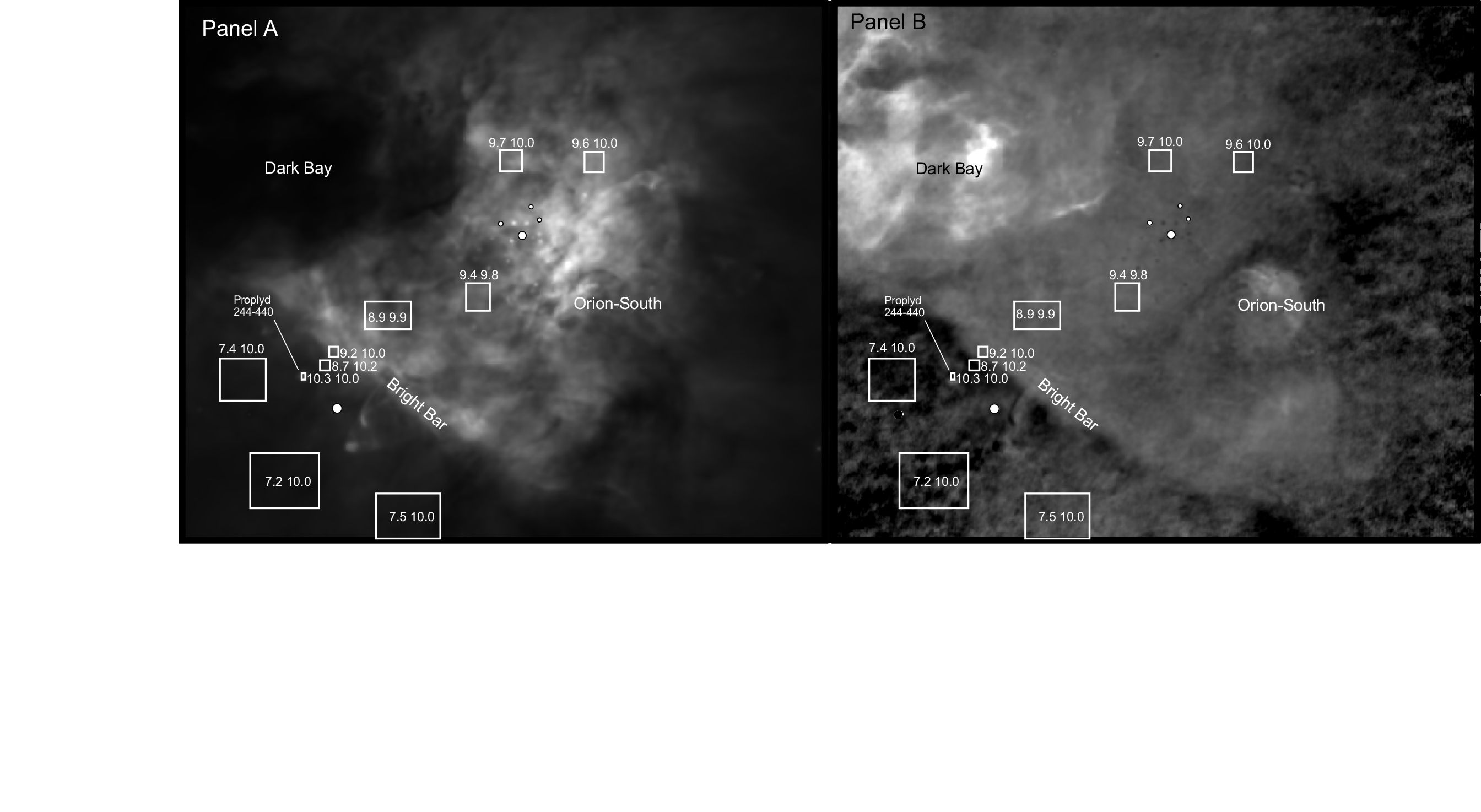
Figure 13: This pair of of 353″$\times$295″ images of the Huygens Region shows the full FOV image of the MUSE database (Weilbacher et al., 2015) in H$\alpha$ in Panel A and the c_VLA/c_MUSE results described in Section A.2 in Panel B. North is up and east to the left. The brightest four of the Trapezium stars are shown as filled circles as is $\theta^{2}$ Ori A in the southeast. The H$\alpha$ image has been degraded to 1$\aas@@fstack{\prime\prime}$83 $\times$ 1$\aas@@fstack{\prime\prime}$65 FWHM and both panels have a scale of 0$\aas@@fstack{\prime\prime}$5 per pixel. The c_VLA/c_MUSE results were calculated with a fixed temperature of 10000 K. The sample regions subjected to a detailed analysis Section A.3 are shown as boxes. Within or near the boxes the left-hand number is the temperature derived from the MUSE [N ii]  auroral and nebular lines in units of 1000 K while the right-hand number is the temperature, in the same units, derived for the H⁺ emission, using the c_VLA/ c_MUSE  results. The sample centred on the bright portion of proplyd 244-440 is also shown, to the northeast of $\theta^{2}$ Ori A.

A.3 Using c_VLA/c_MUSE as a temperature indicator

The intrinsic ratio of c_VLA and c_MUSE is dependent on T_e. This means that this ratio can be used to derive T_e for the H⁺ emitting regions, rather than assuming T_e to be the same as that indicated by co-existing collisionally excited forbidden lines. The numerator in the c_VLA/c_MUSE ratio is the more sensitive to temperature. There is a log (t^1.35 $\times$ f_eff) term in the numerator (this is about 0.52$\times$log t) and a t^-1 factor in the I_ν term (both in equation 4). The denominator is less sensitive to temperature as it determines the log g(t) term in equation 5, which is about -0.086$\times$log t.

The right-hand panel of Figure 13 shows a map of c_VLA/c_MUSE calculated with t = 1, while the left-hand panel presents a MUSE H$\alpha$ image degraded to the VLA resolution. The centre of the Huygens Region is about 0.8 and other regions and features are greater or lesser than this.

The values in the Dark Bay and Orion-South region are larger than 1 (reaching a peak of 2.4 in the Dark Bay and 1.2 in Orion-South). O’Dell & Yusef-Zadeh (2000) noted that these regions are where the radio and Balmer line emission don’t originate from the same volumes. In these areas the extinction arises from in front of the volumes producing the optical lines but there is background optical emission that is obscured by an intervening extinction layer. In the case of the Dark Bay the extinction is formed from a dense area within the foreground Veil and is sufficiently optically thick that we don’t see optical emission from near the main ionization front of this deformed-blister nebula. In the Orion-South area we see optical emission from the near side of the optically thick Orion-South cloud and radio emission from both there and the portion of the main ionization front that lies beyond it.

The interpretations of the c_VLA/c_MUSE values for the other regions are more complex. For each spot in the map equation 4 and equation 5 have a unique value of T_e that matches the observed c_VLA/c_MUSE ratio. In general, the ratio drops with increasing temperature, but, there is no uniform absolute value for a given temperature. The temperature must be derived pixel by pixel across the Huygens Region. We call the temperature derived from the H⁺ observations T_e(H⁺).

We divided the Huygens Region into 9 samples as shown in Figure 13. These samples were selected to represent different types of regions in the nebula. For each sample the averaged S(H$\alpha$), S(H$\beta$), and I_ν observations were adopted to calculate the variation of c_VLA/c_MUSE for a range of values of T_e. When the calculated ratio matched the observed ratio, that temperature was adopted and is shown in the panels. This method effectively solves for T_e, independent of the amount of extinction. The scatter in c_VLA/c_MUSE varied from about 5$\%$ to 20$\%$. This scatter led to uncertainties in the derived temperatures of 200 K to 1500 K. A tenth sample, centred on the largest proplyd in the Huygens Region, was also studied in this fashion and is discussed below. Figure 13 also shows the averaged T_e values derived from the MUSE [N ii] lines, which we will call T_e([N II]). We see that the T_e([N II]) values are usually smaller than the T_e(H⁺) values. There are systematic differences between the inner and outer parts of the Huygens Region, where these areas are closer to the Trapezium than the Bright Bar or further, respectively. For the five samples in the inner region the average ratio of T_e([N II])/T_e(H⁺) is 0.94$\pm$0.03 and for the outer four samples it is 0.74$\pm$0.02.

A.4 The extinction curve appears to be different inside and outside the Bright Bar

The H⁺ emission should arise from both the He^o+H⁺ and the He⁺+H⁺ layers and photoionization models predict only small differences of T_e([N II]) and T_e(H⁺), with T_e([N II]) about 10% higher. However, the observed T_e([N II])/T_e(H⁺) ratio is less than unity and is different inside and outside of the Bright Bar. The answer to this riddle probably does not lie in a problem with the basic blister model of the nebula and our ability to calculate T_e in different ionization zones, rather it must lie in the assumptions we have made about the nature of the extinction curve, which determines r. Recall that for each sample region the calculated c_VLA/c_MUSE ratios decreased with increasing assumed temperature. This means that if the ratio derived from the observations is too low, then the derived T_e(H⁺) value is too high.

In order to derive T_e(H⁺) values that are no greater than the T_e([N II]) temperatures, we need to look for causes of a non-representative value of c_VLA/c_MUSE. The quantity r occurs in the numerator in the derivation of c_VLA/c_MUSE and we have used the Blagrave et al. (2007) value of 0.22 throughout. Adjusting the derived c_VLA/c_MUSE to give lower temperatures means using a larger value of r. To match the c_VLA/c_MUSE to that expected from T_e([N II]) would mean using r = 0.23$\pm$0.02 for the Inner samples and 0.36$\pm$0.07 for the outer samples.

It appears that the extinction curve is very different for the inner and outer samples. The value of 0.23$\pm$0.02 is well within the apparent uncertainty of the extinction curve as shown in Figure 3 of Blagrave et al. (2007). Therefore it appears that the c_VLA/c_MUSE ratio support the unusual extinction curve in the Huygens Region as determined by Blagrave et al. (2007). Our r value for the outer samples agrees well with the extinction curve difference of 0.35 for the ISM presented in AGN3.

This leads us to the important conclusion that in the outer samples the ISM extinction curve applies. It is generally thought that the more grey extinction that applies to the Huygens Region is a result of either destruction of the small size grains within the distribution of sizes or the building up of larger grains by the coalescing of smaller grains. In any event, these results indicate that the nature of the interstellar particles causing the extinction in the Huygens Region abruptly changes at the Bright Bar. This property is one more fact that must be accommodated when building a more accurate model of the Huygens Region.

There are important caveats about using the c_VLA/c_MUSE ratios. (O’Dell, 2009b) pointed out that filter images (for example the WFPC2 F487N filter) measures all of the components, that from the MIF, the backscattered red component, and emission from the Blue Layer. The ratio of the backscattered component to the MIF component (around 0.1) will artificially enhance the observed surface brightness of H$\beta$ and thus lead to a c_VLA result that is too small. The backscattered component is less important in determination of c_MUSE because it will only enter as the difference in the backscattering at the H$\alpha$ and H$\beta$ lines. Therefore, a correction for backscattering would systematically increase the expected c_VLA/c_MUSE ratio by about 10% and raise the c_VLA/c_MUSE derived T_e(H⁺) value. This would broaden the disagreement in the T_e([N ii]|) and T_e(c_VLA/c_MUSE) results, which argues that backscattering doesn’t vitiate the c_VLA/c_MUSE approach. The Blue Layer emission will enhance both the emission line radio surface brightnesses, which argues that the Blue Layer contamination is not important. However, in Section 4.1 we saw that outside of the Bright Bar, the Blue Layer emission became important for [N ii]. Since we do not know the density and temperature of the Blue Layer, we cannot estimate its effect on our T_e(H⁺) results.

It is noteworthy that in a recent study by McLeod et al. (2016) it was found that the proplyds outside of the Bright Bar occupy a different [S[S ii]+ S[S iii]]/S(H$\beta$) versus S[O ii]/ S[O iii] space than those lying inside that boundary. Their index was derived using extinction corrected surface brightness where the H$\alpha$/Hb method was used. If the extinction curve is steeper outside the Bright Bar, this property should be re-examined. The largest proplyd in the Huygens Region is 244-440, which also lies outside the Bright Bar, and was included in our c_VLA/c_MUSE study. Not only is it the proplyd with the largest apparent size, it is clearly photoionized by $\theta^{2}$ Ori A (the bright rim of the proplyd faces that star). In this case, the T_e([N II])  value (t=1.03$\pm$0.04) agrees well with the T_e([N II]) value (t=1.00$\pm$0.1), indicating that this proplyd is in a region where the inner-Huygens Region extinction curve applies, even though its position projects to outside the Bright Bar.

References

- Abel et al. (2016) Abel, N. P., Ferland, G. J., O’Dell, C. R., Troland, T. H., 2016, ApJ, 819, 136
- Ascasibar et al. (2011) Ascasibar, Y., et al., 2011, MNRAS, 416, 1546
- Baldwin et al. (1991) Baldwin, J. A., Ferland, G. J., Martin, P. G., Corbin, M. R., Cota, S. A., Peterson, B. M., Slettebak, A., 1991, ApJ, 374, 580 (BFM)
- Bally et al. (2000) Bally, J., O’Dell, C. R., McCaughrean, M. J. 2000, AJ, 119, 2119
- Blagrave et al. (2007) Blagrave, K. P. M., Martin, P. G., Rubin, R. H., Dufour, R. J., Baldwin, J. A., Hester, J. J., Walter, D. K., 2007, ApJ, 655, 299
- Cantó et al. (1998) Cantó, J., Raga, A., Steffen, W., Shapiro, P. R., 1998, ApJ, 502, 695
- Doi et al. (2002) Doi, T., O’Dell, C. R., Hartigan, P., 2002, AJ, 124, 445
- Doi et al. (2004) Doi, T., O’Dell, C. R., Hartigan, P., 2004, AJ, 127, 3456
- Ferland et al. (2016) Ferland, G. J., Henney, W. J., O’Dell, C. R., Peimbert, M. 2016, RMxAA, 52, no. 2, in press
- Ferland et al. (2013) Ferland, G. J., Porter, R. L., van Hoof, P. A. M., 2013, RMxAA, 49, 137
- García-Díaz & Henney (2007) García-Díaz, Ma.-T., Henney, W. J., 2007, AJ, 133, 952
- García-Díaz et al. (2008) García-Díaz, Ma.-T., Henney, W. J., López, J. A., Doi, T., 2008, RMxAA, 44, 181
- Gingerich (1982) Gingerich, O., 1982, Ann. NY Acad. Sci., 395, 308
- Goicoechea (2015) Goicoechea, J. R., et al., 2015, ApJ, 812, 75
- Goudis (1982) Goudis, C. 1982, The Orion complex: A case study of interstellar matter (Dordrecht, Netherlands, D. Reidel Publishing Co.), Astrophysics and Space Science Library,Volume 90
- Henney (1994) Henney, W. J., 1994, RMxAA, 29, 192
- Henney (2005a) Henney, W. J., Arthur, S. J., García-Díaz, M. T. 2005, ApJ, 627, 813
- Henney (2005b) Henney, W. J., et al. 2005, ApJ, 621, 328
- Henney (2007) Henney, W. J., et al. 2007, AJ, 133, 2192
- Hillenbrand (1997) Hillenbrand, L. A., 1997, AJ 113, 1733
- Jones (1992) Jones, M. R., 1992, Ph.D. thesis, Rice University
- McLeod et al. (2016) McLeod, A. F., Weilbacher, P. M., Ginsburg, A., Dale, J. E., Ramsay, S., Testi, L., 2015, MNRAS, 455, 4057
- Medina et al. (2014) Medina, S.-N. X., Arthur, S. J., Henney, W. J., Mellema, G, Gazol, A., 2014, MNRAS, 445, 1797
- Mellama et al. (2006) Mellama, G., Arthur, S. J., Henney, W. J., Iliev, I. T., Shapiro, P. R., 2006, ApJ, 647, 397
- Mesa-Delgado et al. (2008) Mesa-Delgado, A., Esteban, C., García-Rojas, J. 2008, ApJ, 675, 389
- Mesa-Delgado et al. (2011) Mesa-Delgado, A., et al., 2011, MNRAS, 417, 420
- Muench, et al. (2008) Muench. A.,Getman, K., Hillenbrand, L., Preibisch, T., 2008, in Handbook of Star Forming Regions: The Northern Sky, Vol. 1, ed. B. Reipurth (San Francisco, CA: ASP), 483
- Münch (1958) Münch, G., 1958, RevModPhys, 30, 1035
- Núñez-Diaz et al. (2012) Núñez-Díaz, M. et al., 2012, MNRAS, 421, 3399
- O’Dell (2000) O’Dell, C.R., 2000, AJ, 119, 2311
- O’Dell (2001) O’Dell, C.R., 2001, ARA&A, 39, 99
- O’Dell (2009a) O’Dell, C.R., 2009a, PASP, 121, 428
- O’Dell et al. (1992) O’Dell, C. R., Walter, D. K., Dufour, R. J., 1992, ApJ, 399, L67
- O’Dell et al. (1997) O’Dell, C. R., et al., 1997, AJ, 114, 2016
- O’Dell (2009b) O’Dell, C.R., et al., 2009b, AJ, 137, 367
- O’Dell et al. (2015) O’Dell, C.R., et al., 2015, AJ, 115, 108
- O’Dell & Harris (2010) O’Dell, C. R., & Harris, J. A., 2010, AJ, 140, 985
- O’Dell et al. (2008) O’Dell, C. R., Muench, A., Smith, N., Zapata, L., 2008, in Handbook of Star Forming Regions: The Northern Sky, Vol. 1, ed. B. Reipurth (San Francisco, CA: ASP), 544
- O’Dell et al. (2003) O’Dell, C. R., Peimbert, M., Peimbert, A., 2003, AJ, 125, 2590
- O’Dell & Wong (1996) O’Dell, C. R., Wong, Shui-Kwan 1996, AJ, 111, 846
- O’Dell & Yusef-Zadeh (2000) O’Dell, C. R., & Yusef-Zadeh, F., 2000, AJ, 120, 382
- Osterbrock & Ferland (2006) Osterbrock, D. E., & Ferland, G. J., 2006, Astrophysics of Gaseous Nebulae and Active Galactic Nuclei (second edition), University Science Books (Mill Valley) (AGN3)
- Peimbert (1967) Peimbert, M., 1967, ApJ, 150, 825
- Peimbert (1969) Peimbert, M., Costero, R. 1969,BOTT,5,3
- Pellegrini et al. (2009) Pellegrini, E. W., et al., 2009, ApJ, 693, 285
- Shaw et al. (2009) Shaw, G., et al., 2009, ApJ, 701, 677
- Walmsley (2000) Walmsley, C. M., et al., 2000, A&A, 364, 301
- Weilbacher et al. (2015) Weilbacher, P. M., et al., 2015, A&A, 582, A114
- van der Werf & Goss (1989) van der Werf, P. P., & Goss, W. M., 1989, A&A, 224, 209
- van der Werf et al. (1996) van der Werf, P. P., Stutzki, J., Sternberg, A., Krabbe, S. 1996, A&A, 313, 633
- van der Werf et al. (2013) van der Werf, P. P., Goss, W. M., & O’Dell, C. R. 2013 ApJ, 762, 101
- van der Wiel et al. (2009) van der Wiel, M. H. D., et al., 2009, A&A, 498, 161
- Wen & O’Dell (1995) Wen, Z., O’Dell, C. R., 1995, ApJ, 438, 784
- Wilson et al. (1959) Wilson, O. C., Münch, G., Flather, E. M., Coffeen, M. F., 1959, ApJS, 4, 199
- Wilson et al. (1997) Wilson, T. L., Filges, L., Codella, C., Reich, W., Reich, P., 1997, A&A, 327, 1177
- Wilson et al. (2015) Wilson, T. L., Bania, T. M., Balser, Dana S., 2015, ApJ, 812, 45