Combinatorial Multi-Armed Bandit with General Reward Functions

Abstract

In this paper, we study the stochastic combinatorial multi-armed bandit (CMAB) framework that allows a general nonlinear reward function, whose expected value may not depend only on the means of the input random variables but possibly on the entire distributions of these variables. Our framework enables a much larger class of reward functions such as the $\max()$ function and nonlinear utility functions. Existing techniques relying on accurate estimations of the means of random variables, such as the upper confidence bound (UCB) technique, do not work directly on these functions. We propose a new algorithm called stochastically dominant confidence bound (SDCB), which estimates the distributions of underlying random variables and their stochastically dominant confidence bounds. We prove that SDCB can achieve $O(\log T)$ distribution-dependent regret and $\tilde{O}(\sqrt{T})$ distribution-independent regret, where $T$ is the time horizon. We apply our results to the $K$-MAX problem and expected utility maximization problems. In particular, for $K$-MAX, we provide the first polynomial-time approximation scheme (PTAS) for its offline problem, and give the first $\tilde{O}(\sqrt{T})$ bound on the $(1-\epsilon)$-approximation regret of its online problem, for any $\epsilon>0$.

1 Introduction

Stochastic multi-armed bandit (MAB) is a classical online learning problem typically specified as a player against $m$ machines or arms. Each arm, when pulled, generates a random reward following an unknown distribution. The task of the player is to select one arm to pull in each round based on the historical rewards she collected, and the goal is to collect cumulative reward over multiple rounds as much as possible. In this paper, unless otherwise specified, we use MAB to refer to stochastic MAB.

MAB problem demonstrates the key tradeoff between exploration and exploitation: whether the player should stick to the choice that performs the best so far, or should try some less explored alternatives that may provide better rewards. The performance measure of an MAB strategy is its cumulative regret, which is defined as the difference between the cumulative reward obtained by always playing the arm with the largest expected reward and the cumulative reward achieved by the learning strategy. MAB and its variants have been extensively studied in the literature, with classical results such as tight $\Theta(\log T)$ distribution-dependent and $\Theta(\sqrt{T})$ distribution-independent upper and lower bounds on the regret in $T$ rounds [19, 2, 1].

An important extension to the classical MAB problem is combinatorial multi-armed bandit (CMAB). In CMAB, the player selects not just one arm in each round, but a subset of arms or a combinatorial object in general, referred to as a super arm, which collectively provides a random reward to the player. The reward depends on the outcomes from the selected arms. The player may observe partial feedbacks from the selected arms to help her in decision making. CMAB has wide applications in online advertising, online recommendation, wireless routing, dynamic channel allocations, etc., because in all these settings the action unit is a combinatorial object (e.g. a set of advertisements, a set of recommended items, a route in a wireless network, and an allocation between channels and users), and the reward depends on unknown stochastic behaviors (e.g. users’ click through behaviors, wireless transmission quality, etc.). Therefore CMAB has attracted a lot of attention in online learning research in recent years [12, 8, 22, 15, 7, 16, 18, 17, 23, 9].

Most of these studies focus on linear reward functions, for which the expected reward for playing a super arm is a linear combination of the expected outcomes from the constituent base arms. Even for studies that do generalize to non-linear reward functions, they typically still assume that the expected reward for choosing a super arm is a function of the expected outcomes from the constituent base arms in this super arm [8, 17]. However, many natural reward functions do not satisfy this property. For example, for the function $\max()$, which takes a group of variables and outputs the maximum one among them, its expectation depends on the full distributions of the input random variables, not just their means. Function $\max()$ and its variants underly many applications. As an illustrative example, we consider the following scenario in auctions: the auctioneer is repeatedly selling an item to $m$ bidders; in each round the auctioneer selects $K$ bidders to bid; each of the $K$ bidders independently draws her bid from her private valuation distribution and submits the bid; the auctioneer uses the first-price auction to determine the winner and collects the largest bid as the payment. The goal of the auctioneer is to gain as high cumulative payments as possible. We refer to this problem as the $K$-MAX bandit problem, which cannot be effectively solved in the existing CMAB framework.

Beyond the $K$-MAX problem, many expected utility maximization (EUM) problems are studied in stochastic optimization literature [27, 20, 21, 4]. The problem can be formulated as maximizing ${\mathbb{E}}[u(\sum_{i\in S}X_{i})]$ among all feasible sets $S$, where $X_{i}$’s are independent random variables and $u(\cdot)$ is a utility function. For example, $X_{i}$ could be the random delay of edge $e_{i}$ in a routing graph, $S$ is a routing path in the graph, and the objective is maximizing the utility obtained from any routing path, and typically the shorter the delay, the larger the utility. The utility function $u(\cdot)$ is typically nonlinear to model risk-averse or risk-prone behaviors of users (e.g. a concave utility function is often used to model risk-averse behaviors). The non-linear utility function makes the objective function much more complicated: in particular, it is no longer a function of the means of the underlying random variables $X_{i}$’s. When the distributions of $X_{i}$’s are unknown, we can turn EUM into an online learning problem where the distributions of $X_{i}$’s need to be learned over time from online feedbacks, and we want to maximize the cumulative reward in the learning process. Again, this is not covered by the existing CMAB framework since only learning the means of $X_{i}$’s is not enough.

In this paper, we generalize the existing CMAB framework with semi-bandit feedbacks to handle general reward functions, where the expected reward for playing a super arm may depend more than just the means of the base arms, and the outcome distribution of a base arm can be arbitrary. This generalization is non-trivial, because almost all previous works on CMAB rely on estimating the expected outcomes from base arms, while in our case, we need an estimation method and an analytical tool to deal with the whole distribution, not just its mean. To this end, we turn the problem into estimating the cumulative distribution function (CDF) of each arm’s outcome distribution. We use stochastically dominant confidence bound (SDCB) to obtain a distribution that stochastically dominates the true distribution with high probability, and hence we also name our algorithm SDCB. We are able to show $O(\log T)$ distribution-dependent and $\tilde{O}(\sqrt{T})$ distribution-independent regret bounds in $T$ rounds. Furthermore, we propose a more efficient algorithm called Lazy-SDCB, which first executes a discretization step and then applies SDCB on the discretized problem. We show that Lazy-SDCB also achieves $\tilde{O}(\sqrt{T})$ distribution-independent regret bound. Our regret bounds are tight with respect to their dependencies on $T$ (up to a logarithmic factor for distribution-independent bounds). To make our scheme work, we make a few reasonable assumptions, including boundedness, monotonicity and Lipschitz-continuity of the reward function, and independence among base arms. We apply our algorithms to the $K$-MAX and EUM problems, and provide efficient solutions with concrete regret bounds. Along the way, we also provide the first polynomial time approximation scheme (PTAS) for the offline $K$-MAX problem, which is formulated as maximizing ${\mathbb{E}}[\max_{i\in S}X_{i}]$ subject to a cardinality constraint $|S|\leq K$, where $X_{i}$’s are independent nonnegative random variables.

To summarize, our contributions include: (a) generalizing the CMAB framework to allow a general reward function whose expectation may depend on the entire distributions of the input random variables; (b) proposing the SDCB algorithm to achieve efficient learning in this framework with near-optimal regret bounds, even for arbitrary outcome distributions; (c) giving the first PTAS for the offline $K$-MAX problem. Our general framework treats any offline stochastic optimization algorithm as an oracle, and effectively integrates it into the online learning framework.

Related Work.

As already mentioned, most relevant to our work are studies on CMAB frameworks, among which [12, 16, 18, 9] focus on linear reward functions while [8, 17] look into non-linear reward functions. In particular, Chen et al. [8] look at general non-linear reward functions and Kveton et al. [17] consider specific non-linear reward functions in a conjunctive or disjunctive form, but both papers require that the expected reward of playing a super arm is determined by the expected outcomes from base arms.

The only work in combinatorial bandits we are aware of that does not require the above assumption on the expected reward is [15], which is based on a general Thompson sampling framework. However, they assume that the joint distribution of base arm outcomes is from a known parametric family within known likelihood function and only the parameters are unknown. They also assume the parameter space to be finite. In contrast, our general case is non-parametric, where we allow arbitrary bounded distributions. Although in our known finite support case the distribution can be parametrized by probabilities on all supported points, our parameter space is continuous. Moreover, it is unclear how to efficiently compute posteriors in their algorithm, and their regret bounds depend on complicated problem-dependent coefficients which may be very large for many combinatorial problems. They also provide a result on the $K$-MAX problem, but they only consider Bernoulli outcomes from base arms, much simpler than our case where general distributions are allowed.

There are extensive studies on the classical MAB problem, for which we refer to a survey by Bubeck and Cesa-Bianchi [5]. There are also some studies on adversarial combinatorial bandits, e.g. [26, 6]. Although it bears conceptual similarities with stochastic CMAB, the techniques used are different.

Expected utility maximization (EUM) encompasses a large class of stochastic optimization problems and has been well studied (e.g. [27, 20, 21, 4]). To the best of our knowledge, we are the first to study the online learning version of these problems, and we provide a general solution to systematically address all these problems as long as there is an available offline (approximation) algorithm. The $K$-MAX problem may be traced back to [13], where Goel et al. provide a constant approximation algorithm to a generalized version in which the objective is to choose a subset $S$ of cost at most $K$ and maximize the expectation of a certain knapsack profit.

2 Setup and Notation

Problem Formulation.

We model a combinatorial multi-armed bandit (CMAB) problem as a tuple $(E,{\mathcal{F}},D,R)$, where $E=[m]=\{1,2,\ldots,m\}$ is a set of $m$ (base) arms, ${\mathcal{F}}\subseteq 2^{E}$ is a set of subsets of $E$, $D$ is a probability distribution over $[0,1]^{m}$, and $R$ is a reward function defined on $[0,1]^{m}\times{\mathcal{F}}$. The arms produce stochastic outcomes $X=(X_{1},X_{2},\ldots,X_{m})$ drawn from distribution $D$, where the $i$-th entry $X_{i}$ is the outcome from the $i$-th arm. Each feasible subset of arms $S\in{\mathcal{F}}$ is called a super arm. Under a realization of outcomes $x=(x_{1},\ldots,x_{m})$, the player receives a reward $R(x,S)$ when she chooses the super arm $S$ to play. Without loss of generality, we assume the reward value to be nonnegative. Let $K=\max_{S\in{\mathcal{F}}}|S|$ be the maximum size of any super arm.

Let $X^{(1)},X^{(2)},\ldots$ be an i.i.d. sequence of random vectors drawn from $D$, where $X^{(t)}=(X^{(t)}_{1},\ldots,X^{(t)}_{m})$ is the outcome vector generated in the $t$-th round. In the $t$-th round, the player chooses a super arm $S_{t}\in{\mathcal{F}}$ to play, and then the outcomes from all arms in $S_{t}$, i.e., $\{X^{(t)}_{i}\,|\,i\in S_{t}\}$, are revealed to the player. According to the definition of the reward function, the reward value in the $t$-th round is $R(X^{(t)},S_{t})$. The expected reward for choosing a super arm $S$ in any round is denoted by $r_{D}(S)={\mathbb{E}}_{X\sim D}[R(X,S)]$.

We also assume that for a fixed super arm $S\in{\mathcal{F}}$, the reward $R(x,S)$ only depends on the revealed outcomes $x_{S}=(x_{i})_{i\in S}$. Therefore, we can alternatively express $R(x,S)$ as $R_{S}(x_{S})$, where $R_{S}$ is a function defined on $[0,1]^{S}$.

A learning algorithm ${\mathcal{A}}$ for the CMAB problem selects which super arm to play in each round based on the revealed outcomes in all previous rounds. Let $S^{\mathcal{A}}_{t}$ be the super arm selected by ${\mathcal{A}}$ in the $t$-th round. The goal is to maximize the expected cumulative reward in $T$ rounds, which is ${\mathbb{E}}\left[\sum_{t=1}^{T}R(X^{(t)},S^{\mathcal{A}}_{t})\right]=\sum_{t=1}^{T}{\mathbb{E}}\left[r_{D}(S^{\mathcal{A}}_{t})\right]$. Note that when the underlying distribution $D$ is known, the optimal algorithm ${\mathcal{A}}^{*}$ chooses the optimal super arm $S^{*}=\operatornamewithlimits{argmax}_{S\in{\mathcal{F}}}\{r_{D}(S)\}$ in every round. The quality of an algorithm ${\mathcal{A}}$ is measured by its regret in $T$ rounds, which is the difference between the expected cumulative reward of the optimal algorithm ${\mathcal{A}}^{*}$ and that of ${\mathcal{A}}$:

$$\mathsf{Reg}_{D}^{\mathcal{A}}(T)=T\cdot r_{D}(S^{*})-\sum_{t=1}^{T}{\mathbb{E}}\left[r_{D}(S^{\mathcal{A}}_{t})\right].$$

For some CMAB problem instances, the optimal super arm $S^{*}$ may be computationally hard to find even when the distribution $D$ is known, but efficient approximation algorithms may exist, i.e., an $\alpha$-approximate ($0<\alpha\leq 1$) solution $S^{\prime}\in{\mathcal{F}}$ which satisfies $r_{D}(S^{\prime})\geq\alpha\cdot\max_{S\in{\mathcal{F}}}\{r_{D}(S)\}$ can be efficiently found given $D$ as input. We will provide the exact formulation of our requirement on such an $\alpha$-approximation computation oracle shortly. In such cases, it is not fair to compare a CMAB algorithm ${\mathcal{A}}$ with the optimal algorithm ${\mathcal{A}}^{*}$ which always chooses the optimal super arm $S^{*}$. Instead, we define the $\alpha$-approximation regret of an algorithm ${\mathcal{A}}$ as

$$\mathsf{Reg}_{D,\alpha}^{\mathcal{A}}(T)=T\cdot\alpha\cdot r_{D}(S^{*})-\sum_{t=1}^{T}{\mathbb{E}}\left[r_{D}(S^{\mathcal{A}}_{t})\right].$$

As mentioned, almost all previous work on CMAB requires that the expected reward $r_{D}(S)$ of a super arm $S$ depends only on the expectation vector $\mu=(\mu_{1},\ldots,\mu_{m})$ of outcomes, where $\mu_{i}={\mathbb{E}}_{X\sim D}[X_{i}]$. This is a strong restriction that cannot be satisfied by a general nonlinear function $R_{S}$ and a general distribution $D$. The main motivation of this work is to remove this restriction.

Assumptions.

Throughout this paper, we make several assumptions on the outcome distribution $D$ and the reward function $R$.

Assumption 1 (Independent outcomes from arms).

The outcomes from all $m$ arms are mutually independent, i.e., for $X\sim D$, $X_{1},X_{2},\ldots,X_{m}$ are mutually independent. We write $D$ as $D=D_{1}\times D_{2}\times\cdots\times D_{m}$, where $D_{i}$ is the distribution of $X_{i}$.

We remark that the above independence assumption is also made for past studies on the offline EUM and K-MAX problems [27, 20, 21, 4, 13], so it is not an extra assumption for the online learning case.

Assumption 2 (Bounded reward value).

There exists $M>0$ such that for any $x\in[0,1]^{m}$ and any $S\in{\mathcal{F}}$, we have $0\leq R(x,S)\leq M$.

Assumption 3 (Monotone reward function).

If two vectors $x,x^{\prime}\in[0,1]^{m}$ satisfy $x_{i}\leq x_{i}^{\prime}$ ($\forall i\in[m]$), then for any $S\in{\mathcal{F}}$, we have $R(x,S)\leq R(x^{\prime},S)$.

Computation Oracle for Discrete Distributions with Finite Supports.

We require that there exists an $\alpha$-approximation computation oracle ($0<\alpha\leq 1$) for maximizing $r_{D}(S)$, when each $D_{i}$ ($i\in[m]$) has a finite support. In this case, $D_{i}$ can be fully described by a finite set of numbers (i.e., its support $\{v_{i,1},v_{i,2},\ldots,v_{i,s_{i}}\}$ and the values of its cumulative distribution function (CDF) $F_{i}$ on the supported points: $F_{i}(v_{i,j})=\Pr_{X_{i}\sim D_{i}}\left[X_{i}\leq v_{i,j}\right](j\in[s_{i}])$). The oracle takes such a representation of $D$ as input, and can output a super arm $S^{\prime}=\mathsf{Oracle}(D)\in{\mathcal{F}}$ such that $r_{D}(S^{\prime})\geq\alpha\cdot\max_{S\in{\mathcal{F}}}\{r_{D}(S)\}$.

3 SDCB Algorithm

Algorithm 1 SDCB (Stochastically dominant confidence bound)

1:  Throughout the algorithm, for each arm $i\in[m]$, maintain: (i) a counter $T_{i}$ which stores the number of times arm $i$ has been played so far, and (ii) the empirical distribution $\hat{D}_{i}$ of the observed outcomes from arm $i$ so far, which is represented by its CDF $\hat{F}_{i}$

2:  // Initialization

3:  for $i=1$ to $m$ do

4:     // Action in the $i$-th round

5:     Play a super arm $S_{i}$ that contains arm $i$

6:     Update $T_{j}$ and $\hat{F}_{j}$ for each $j\in S_{i}$

7:  end for

8:  for $t=m+1,m+2,\ldots$ do

9:     // Action in the $t$-th round

10:      For each $i\in[m]$, let $\underaccent{{\cc@style\underline{\mskip 10.0mu}}}{D}_{i}$ be a distribution whose CDF $\underaccent{{\cc@style\underline{\mskip 10.0mu}}}{F}_{i}$ is

$$\underaccent{{\cc@style\underline{\mskip 10.0mu}}}{F}_{i}(x)=\begin{cases}\max\{\hat{F}_{i}(x)-\sqrt{\frac{3\ln t}{2T_{i}}},0\},&0\leq x<1\\ 1,&x=1\end{cases}$$

11:      Play the super arm $S_{t}\leftarrow\mathsf{Oracle}(\underaccent{{\cc@style\underline{\mskip 10.0mu}}}{D})$, where $\underaccent{{\cc@style\underline{\mskip 10.0mu}}}{D}=\underaccent{{\cc@style\underline{\mskip 10.0mu}}}{D}_{1}\times\underaccent{{\cc@style\underline{\mskip 10.0mu}}}{D}_{2}\times\cdots\times\underaccent{{\cc@style\underline{\mskip 10.0mu}}}{D}_{m}$

12:     Update $T_{j}$ and $\hat{F}_{j}$ for each $j\in S_{t}$

13:  end for

We present our algorithm stochastically dominant confidence bound (SDCB) in Algorithm 1. Throughout the algorithm, we store, in a variable $T_{i}$, the number of times the outcomes from arm $i$ are observed so far. We also maintain the empirical distribution $\hat{D}_{i}$ of the observed outcomes from arm $i$ so far, which can be represented by its CDF $\hat{F}_{i}$: for $x\in[0,1]$, the value of $\hat{F}_{i}(x)$ is just the fraction of the observed outcomes from arm $i$ that are no larger than $x$. Note that $\hat{F}_{i}$ is always a step function which has “jumps” at the points that are observed outcomes from arm $i$. Therefore it suffices to store these discrete points as well as the values of $\hat{F}_{i}$ at these points in order to store the whole function $\hat{F}_{i}$. Similarly, the later computation of stochastically dominant CDF $\underaccent{{\cc@style\underline{\mskip 10.0mu}}}{F}_{i}$ (line 10) only requires computation at these points, and the input to the offline oracle only needs to provide these points and corresponding CDF values (line 11).

The algorithm starts with $m$ initialization rounds in which each arm is played at least once (lines 2-7). In the $t$-th round ($t>m$), the algorithm consists of three steps. First, it calculates for each $i\in[m]$ a distribution $\underaccent{{\cc@style\underline{\mskip 10.0mu}}}{D}_{i}$ whose CDF $\underaccent{{\cc@style\underline{\mskip 10.0mu}}}{F}_{i}$ is obtained by lowering the CDF $\hat{F}_{i}$ (line 10). The second step is to call the $\alpha$-approximation oracle with the newly constructed distribution $\underaccent{{\cc@style\underline{\mskip 10.0mu}}}{D}=\underaccent{{\cc@style\underline{\mskip 10.0mu}}}{D}_{1}\times\cdots\times\underaccent{{\cc@style\underline{\mskip 10.0mu}}}{D}_{m}$ as input (line 11), and thus the super arm $S_{t}$ output by the oracle satisfies $r_{\underaccent{{\cc@style\underline{\mskip 10.0mu}}}{D}}(S_{t})\geq\alpha\cdot\max_{S\in{\mathcal{F}}}\{r_{\underaccent{{\cc@style\underline{\mskip 10.0mu}}}{D}}(S)\}$. Finally, the algorithm chooses the super arm $S_{t}$ to play, observes the outcomes from all arms in $S_{t}$, and updates $T_{j}$’s and $\hat{F}_{j}$’s accordingly for each $j\in S_{t}$.

The idea behind our algorithm is the optimism in the face of uncertainty principle, which is the key principle behind UCB-type algorithms. Our algorithm ensures that with high probability we have $\underaccent{{\cc@style\underline{\mskip 10.0mu}}}{F}_{i}(x)\leq F_{i}(x)$ simultaneously for all $i\in[m]$ and all $x\in[0,1]$, where $F_{i}$ is the CDF of the outcome distribution $D_{i}$. This means that each $\underaccent{{\cc@style\underline{\mskip 10.0mu}}}{D}_{i}$ has first-order stochastic dominance over $D_{i}$. Then from the monotonicity property of $R(x,S)$ (Assumption 3) we know that $r_{\underaccent{{\cc@style\underline{\mskip 10.0mu}}}{D}}(S)\geq r_{D}(S)$ holds for all $S\in{\mathcal{F}}$ with high probability. Therefore $\underaccent{{\cc@style\underline{\mskip 10.0mu}}}{D}$ provides an “optimistic” estimation on the expected reward from each super arm.

Regret Bounds.

We prove $O(\log T)$ distribution-dependent and $O(\sqrt{T\log T})$ distribution-independent upper bounds on the regret of SDCB (Algorithm 1).

We call a super arm $S$ bad if $r_{D}(S)<\alpha\cdot r_{D}(S^{*})$. For each super arm $S$, we define

$$\Delta_{S}=\max\{\alpha\cdot r_{D}(S^{*})-r_{D}(S),0\}.$$

Let ${\mathcal{F}}_{\mathrm{B}}=\{S\in{\mathcal{F}}\mid\Delta_{S}>0\}$, which is the set of all bad super arms. Let $E_{\mathrm{B}}\subseteq[m]$ be the set of arms that are contained in at least one bad super arm. For each $i\in E_{\mathrm{B}}$, we define

$$\Delta_{i,\min}=\min\{\Delta_{S}\mid S\in{\mathcal{F}}_{\mathrm{B}},i\in S\}.$$

Recall that $M$ is an upper bound on the reward value (Assumption 2) and $K=\max_{S\in{\mathcal{F}}}|S|$.

Theorem 1.

A distribution-dependent upper bound on the $\alpha$-approximation regret of SDCB (Algorithm 1) in $T$ rounds is

$$M^{2}K\sum_{i\in E_{\mathrm{B}}}\frac{2136}{\Delta_{i,\min}}\ln T+\left(\frac{\pi^{2}}{3}+1\right)\alpha Mm,$$

and a distribution-independent upper bound is

$$93M\sqrt{mKT\ln T}+\left(\frac{\pi^{2}}{3}+1\right)\alpha Mm.$$

The proof of Theorem 1 is given in Appendix A.1. The main idea is to reduce our analysis on general reward functions satisfying Assumptions 1-3 to the one in [18] that deals with the summation reward function $R(x,S)=\sum_{i\in S}x_{i}$. Our analysis relies on the Dvoretzky-Kiefer-Wolfowitz inequality [10, 24], which gives a uniform concentration bound on the empirical CDF of a distribution.

Applying Our Algorithm to the Previous CMAB Framework.

Although our focus is on general reward functions, we note that when SDCB is applied to the previous CMAB framework where the expected reward depends only on the means of the random variables, it can achieve the same regret bounds as the previous combinatorial upper confidence bound (CUCB) algorithm in [8, 18].

Let $\mu_{i}={\mathbb{E}}_{X\sim D}[X_{i}]$ be arm $i$’s mean outcome. In each round CUCB calculates (for each arm $i$) an upper confidence bound $\bar{\mu}_{i}$ on $\mu_{i}$, with the essential property that $\mu_{i}\leq\bar{\mu}_{i}\leq\mu_{i}+\Lambda_{i}$ holds with high probability, for some $\Lambda_{i}>0$. In SDCB, we use $\underaccent{{\cc@style\underline{\mskip 10.0mu}}}{D}_{i}$ as a stochastically dominant confidence bound of $D_{i}$. We can show that $\mu_{i}\leq{\mathbb{E}}_{Y_{i}\sim\underaccent{{\cc@style\underline{\mskip 10.0mu}}}{D}_{i}}[Y_{i}]\leq\mu_{i}+\Lambda_{i}$ holds with high probability, with the same interval length $\Lambda_{i}$ as in CUCB. (The proof is given in Appendix A.2.) Hence, the analysis in [8, 18] can be applied to SDCB, resulting in the same regret bounds.We further remark that in this case we do not need the three assumptions stated in Section 2 (in particular the independence assumption on $X_{i}$’s): the summation reward case just works as in [18] and the nonlinear reward case relies on the properties of monotonicity and bounded smoothness used in [8].

4 Improved SDCB Algorithm by Discretization

In Section 3, we have shown that our algorithm SDCB achieves near-optimal regret bounds. However, that algorithm might suffer from large running time and memory usage. Note that, in the $t$-th round, an arm $i$ might have been observed $t-1$ times already, and it is possible that all the observed values from arm $i$ are different (e.g., when arm $i$’s outcome distribution $D_{i}$ is continuous). In such case, it takes $\Theta(t)$ space to store the empirical CDF $\hat{F}_{i}$ of the observed outcomes from arm $i$, and both calculating the stochastically dominant CDF $\underaccent{{\cc@style\underline{\mskip 10.0mu}}}{F}_{i}$ and updating $\hat{F}_{i}$ take $\Theta(t)$ time. Therefore, the worst-case space usage of SDCB in $T$ rounds is $\Theta(T)$, and the worst-case running time is $\Theta(T^{2})$ (ignoring the dependence on $m$ and $K$); here we do not count the time and space used by the offline computation oracle.

In this section, we propose an improved algorithm Lazy-SDCB which reduces the worst-case memory usage and running time to $O(\sqrt{T})$ and $O(T^{3/2})$, respectively, while preserving the $O(\sqrt{T\log T})$ distribution-independent regret bound. To this end, we need an additional assumption on the reward function:

Assumption 4 (Lipschitz-continuous reward function).

There exists $C>0$ such that for any $S\in{\mathcal{F}}$ and any $x,x^{\prime}\in[0,1]^{m}$, we have $\left|R(x,S)-R(x^{\prime},S)\right|\leq C\|x_{S}-x_{S}^{\prime}\|_{1}$, where $\|x_{S}-x_{S}^{\prime}\|_{1}=\sum_{i\in S}|x_{i}-x_{i}^{\prime}|$.

We first describe the algorithm when the time horizon $T$ is known in advance. The algorithm is summarized in Algorithm 2. We perform a discretization on the distribution $D=D_{1}\times\cdots\times D_{m}$ to obtain a discrete distribution $\tilde{D}=\tilde{D}_{1}\times\cdots\times\tilde{D}_{m}$ such that (i) for $\tilde{X}\sim\tilde{D}$, $\tilde{X}_{1},\ldots,\tilde{X}_{m}$ are also mutually independent, and (ii) every $\tilde{D}_{i}$ is supported on a set of equally-spaced values $\{\frac{1}{s},\frac{2}{s},\ldots,1\}$, where $s$ is set to be $\lceil\sqrt{T}\rceil$. Specifically, we partition $[0,1]$ into $s$ intervals: $I_{1}=[0,\frac{1}{s}],I_{2}=(\frac{1}{s},\frac{2}{s}],\ldots,I_{s-1}=(\frac{s-2}{s},\frac{s-1}{s}],I_{s}=(\frac{s-1}{s},1]$, and define $\tilde{D_{i}}$ as

$$\Pr_{\tilde{X}_{i}\sim\tilde{D}_{i}}[\tilde{X}_{i}=j/s]=\Pr_{X_{i}\sim D_{i}}\left[X_{i}\in I_{j}\right],\qquad j=1,\ldots,s.$$

For the CMAB problem $([m],{\mathcal{F}},D,R)$, our algorithm “pretends” that the outcomes are drawn from $\tilde{D}$ instead of $D$, by replacing any outcome $x\in I_{j}$ by $\frac{j}{s}$ ($\forall j\in[s]$), and then applies SDCB to the problem $([m],{\mathcal{F}},\tilde{D},R)$. Since each $\tilde{D}_{i}$ has a known support $\{\frac{1}{s},\frac{2}{s},\ldots,1\}$, the algorithm only needs to maintain the number of occurrences of each support value in order to obtain the empirical CDF of all the observed outcomes from arm $i$. Therefore, all the operations in a round can be done using $O(s)=O(\sqrt{T})$ time and space, and the total time and space used by Lazy-SDCB are $O(T^{3/2})$ and $O(\sqrt{T})$, respectively.

Algorithm 2 Lazy-SDCB with known time horizon

0:  time horizon $T$

1:  $s\leftarrow\lceil\sqrt{T}\rceil$

2:  $I_{j}\leftarrow\begin{cases}[0,\frac{1}{s}],&j=1\\ (\frac{j-1}{s},\frac{j}{s}],&j=2,\ldots,s\end{cases}$

3:  Invoke SDCB (Algorithm 1) for $T$ rounds, with the following change: whenever observing an outcome $x$ (from any arm), find $j\in[s]$ such that $x\in I_{j}$, and regard this outcome as $\frac{j}{s}$

The discretization parameter $s$ in Algorithm 2 depends on the time horizon $T$, which is why Algorithm 2 has to know $T$ in advance. We can use the doubling trick to avoid the dependency on $T$. We present such an algorithm (without knowing $T$) in Algorithm 3. It is easy to see that Algorithm 3 has the same asymptotic time and space usages as Algorithm 2.

Algorithm 3 Lazy-SDCB without knowing the time horizon

1:  $q\leftarrow\left\lceil\log_{2}m\right\rceil$

2:  In rounds $1,2,\ldots,2^{q}$, invoke Algorithm 2 with input $T=2^{q}$

3:  for $k=q,q+1,q+2,\ldots$ do

4:     In rounds $2^{k}+1,2^{k}+2,\ldots,2^{k+1}$, invoke Algorithm 2 with input $T=2^{k}$

5:  end for

Regret Bounds.

We show that both Algorithm 2 and Algorithm 3 achieve $O(\sqrt{T\log T})$ distribution-independent regret bounds. The full proofs are given in Appendix B. Recall that $C$ is the coefficient in the Lipschitz condition in Assumption 4.

Theorem 2.

Suppose the time horizon $T$ is known in advance. Then the $\alpha$-approximation regret of Algorithm 2 in $T$ rounds is at most

$$93M\sqrt{mKT\ln T}+2CK\sqrt{T}+\left(\frac{\pi^{2}}{3}+1\right)\alpha Mm.$$

Proof Sketch.

The regret consists of two parts: (i) the regret for the discretized CMAB problem $([m],{\mathcal{F}},\tilde{D},R)$, and (ii) the error due to discretization. We directly apply Theorem 1 for the first part. For the second part, a key step is to show $\left|r_{D}(S)-r_{\tilde{D}}(S)\right|\leq CK/s$ for all $S\in{\mathcal{F}}$ (see Appendix B.1). ∎

Theorem 3.

For any time horizon $T\geq 2$, the $\alpha$-approximation regret of Algorithm 3 in $T$ rounds is at most

$$318M\sqrt{mKT\ln T}+7CK\sqrt{T}+10\alpha Mm\ln T.$$

5 Applications

We describe the $K$-MAX problem and the class of expected utility maximization problems as applications of our general CMAB framework.

The $K$-MAX Problem.

In this problem, the player is allowed to select at most $K$ arms from the set of $m$ arms in each round, and the reward is the maximum one among the outcomes from the selected arms. In other words, the set of feasible super arms is ${\mathcal{F}}=\left\{S\subseteq[m]\,\big{|}\,|S|\leq K\right\}$, and the reward function is $R(x,S)=\max_{i\in S}x_{i}$. It is easy to verify that this reward function satisfies Assumptions 2, 3 and 4 with $M=C=1$.

Now we consider the corresponding offline $K$-MAX problem of selecting at most $K$ arms from $m$ independent arms, with the largest expected reward. It can be implied by a result in [14] that finding the exact optimal solution is NP-hard, so we resort to approximation algorithms. We can show, using submodularity, that a simple greedy algorithm can achieve a $(1-1/e)$-approximation. Furthermore, we give the first PTAS for this problem. Our PTAS can be generalized to constraints other than the cardinality constraint $|S|\leq K$, including $s$-$t$ simple paths, matchings, knapsacks, etc. The algorithms and corresponding proofs are given in Appendix C.

Theorem 4.

There exists a PTAS for the offline $K$-MAX problem. In other words, for any constant $\epsilon>0$, there is a polynomial-time $(1-\epsilon)$-approximation algorithm for the offline $K$-MAX problem.

We thus can apply our SDCB algorithm to the $K$-MAX bandit problem and obtain $O(\log T)$ distribution-dependent and $\tilde{O}(\sqrt{T})$ distribution-independent regret bounds according to Theorem 1, or can apply Lazy-SDCB to get $\tilde{O}(\sqrt{T})$ distribution-independent bound according to Theorem 2 or 3.

Streeter and Golovin [26] study an online submodular maximization problem in the oblivious adversary model. In particular, their result can cover the stochastic $K$-MAX bandit problem as a special case, and an $O(K\sqrt{mT\log m})$ upper bound on the $(1-1/e)$-regret can be shown. While the techniques in [26] can only give a bound on the $(1-1/e)$-approximation regret for $K$-MAX, we can obtain the first $\tilde{O}(\sqrt{T})$ bound on the $(1-\epsilon)$-approximation regret for any constant $\epsilon>0$, using our PTAS as the offline oracle. Even when we use the simple greedy algorithm as the oracle, our experiments show that SDCB performs significantly better than the algorithm in [26] (see Appendix D).

Expected Utility Maximization.

Our framework can also be applied to reward functions of the form $R(x,S)=u(\sum_{i\in S}x_{i})$, where $u(\cdot)$ is an increasing utility function. The corresponding offline problem is to maximize the expected utility ${\mathbb{E}}[u(\sum_{i\in S}x_{i})]$ subject to a feasibility constraint $S\in{\mathcal{F}}$. Note that if $u$ is nonlinear, the expected utility may not be a function of the means of the arms in $S$. Following the celebrated von Neumann-Morgenstern expected utility theorem, nonlinear utility functions have been extensively used to capture risk-averse or risk-prone behaviors in economics (see e.g., [11]), while linear utility functions correspond to risk-neutrality.

Li and Deshpande [20] obtain a PTAS for the expected utility maximization (EUM) problem for several classes of utility functions (including for example increasing concave functions which typically indicate risk-averseness), and a large class of feasibility constraints (including cardinality constraint, $s$-$t$ simple paths, matchings, and knapsacks). Similar results for other utility functions and feasibility constraints can be found in [27, 21, 4]. In the online problem, we can apply our algorithms, using their PTASs as the offline oracle. Again, we can obtain the first tight regret bounds on the $(1-\epsilon)$-approximation regret for any $\epsilon>0$, for the class of online EUM problems.

Acknowledgments

Wei Chen was supported in part by the National Natural Science Foundation of China (Grant No. 61433014). Jian Li and Yu Liu were supported in part by the National Basic Research Program of China grants 2015CB358700, 2011CBA00300, 2011CBA00301, and the National NSFC grants 61033001, 61361136003. The authors would like to thank Tor Lattimore for referring to us the DKW inequality.

Appendix

Appendix A Missing Proofs from Section 3

A.1 Proof of Theorem 1

We present the proof of Theorem 1 in four steps. In Section A.1.1, we review the $L_{1}$ distance between two distributions and present a property of it. In Section A.1.2, we review the Dvoretzky-Kiefer-Wolfowitz (DKW) inequality, which is a strong concentration result for empirical CDFs. In Section A.1.3, we prove some key technical lemmas. Then we complete the proof of Theorem 1 in Section A.1.4.

A.1.1 The $L_{1}$ Distance between Two Probability Distributions

For simplicity, we only consider discrete distributions with finite supports – this will be enough for our purpose.

Let $P$ be a probability distribution. For any $x$, let $P(x)=\Pr_{X\sim P}[X=x]$. We write $P=P_{1}\times P_{2}\times\cdots\times P_{n}$ if the (multivariate) random variable $X\sim P$ can be written as $X=(X_{1},X_{2},\ldots,X_{n})$, where $X_{1},\ldots,X_{n}$ are mutually independent and $X_{i}\sim P_{i}$ ($\forall i\in[n]$).

For two distributions $P$ and $Q$, their $L_{1}$ distance is defined as

$$L_{1}(P,Q)=\sum_{x}|P(x)-Q(x)|,$$

where the summation is taken over $x\in\mathsf{supp}(P)\cup\mathsf{supp}(Q)$.

The $L_{1}$ distance has the following property. It is a folklore result and we provide a proof for completeness.

Lemma 1.

Let $P=P_{1}\times P_{2}\times\cdots\times P_{n}$ and $Q=Q_{1}\times Q_{2}\times\cdots\times Q_{n}$ be two probability distributions. Then we have

$$L_{1}(P,Q)\leq\sum_{i=1}^{n}L_{1}(P_{i},Q_{i}).$$ (1)

Proof.

We prove (1) by induction on $n$.

When $n=2$, we have

$$L_{1}(P,Q) =\sum_{x}\sum_{y}|P(x,y)-Q(x,y)|$$

$$=\sum_{x}\sum_{y}|P_{1}(x)P_{2}(y)-Q_{1}(x)Q_{2}(y)|$$

$$\leq\sum_{x}\sum_{y}\left(|P_{1}(x)P_{2}(y)-P_{1}(x)Q_{2}(y)|+|P_{1}(x)Q_{2}(y)-Q_{1}(x)Q_{2}(y)|\right)$$

$$=\sum_{x}P_{1}(x)\sum_{y}|P_{2}(y)-Q_{2}(y)|+\sum_{y}Q_{2}(y)\sum_{x}|P_{1}(x)-Q_{1}(x)|$$

$$=1\cdot L_{1}(P_{2},Q_{2})+1\cdot L_{1}(P_{1},Q_{1})$$

$$=\sum_{i=1}^{2}L_{1}(P_{i},Q_{i}).$$

Here the summation is taken over $x\in\mathsf{supp}(P_{1})\cup\mathsf{supp}(Q_{1})$ and $y\in\mathsf{supp}(P_{2})\cup\mathsf{supp}(Q_{2})$.

Suppose (1) is proved for $n=k-1$ ($k\geq 3$). When $n=k$, using the results for $n=k-1$ and $n=2$, we get

$$L_{1}(P,Q) \leq\sum_{i=1}^{k-2}L_{1}(P_{i},Q_{i})+L_{1}(P_{k-1}\times P_{k},Q_{k-1}\times Q_{k})$$

$$\leq\sum_{i=1}^{k-2}L_{1}(P_{i},Q_{i})+L_{1}(P_{k-1},Q_{k-1})+L_{1}(P_{k},Q_{k})$$

$$=\sum_{i=1}^{k}L_{1}(P_{i},Q_{i}).$$

This completes the proof. ∎

A.1.2 The DKW Inequality

Consider a distribution $D$ with CDF $F(x)$. Let $\hat{F}_{n}(x)$ be the empirical CDF of $n$ i.i.d. samples $X_{1},\ldots,X_{n}$ drawn from $D$, i.e., $\hat{F}_{n}(x)=\frac{1}{n}\sum_{i=1}^{n}\mathds{1}\{X_{i}\leq x\}$ ($x\in{\mathbb{R}}$). Then we have:

Lemma 2 (Dvoretzky-Kiefer-Wolfowitz inequality [10, 24]).

For any $\epsilon>0$ and any $n\in{\mathbb{Z}}_{+}$, we have

$$\Pr\left[\sup_{x\in{\mathbb{R}}}\left|\hat{F}_{n}(x)-F(x)\right|\geq\epsilon\right]\leq 2e^{-2n\epsilon^{2}}.$$

Note that for any fixed $x\in{\mathbb{R}}$, from the Chernoff bound we have $\Pr\left[\left|\hat{F}_{n}(x)-F(x)\right|\geq\epsilon\right]\leq 2e^{-2n\epsilon^{2}}.$ The DKW inequality states a stronger guarantee that the Chernoff concentration holds simultaneously for all $x\in{\mathbb{R}}$.

A.1.3 Technical Lemmas

The following lemma describes some properties of the expected reward $r_{P}(S)={\mathbb{E}}_{X\sim P}[R(X,S)]$.

Lemma 3.

Let $P=P_{1}\times\cdots\times P_{m}$ and $P^{\prime}=P_{1}^{\prime}\times\cdots\times P_{m}^{\prime}$ be two probability distributions over $[0,1]^{m}$. Let $F_{i}$ and $F_{i}^{\prime}$ be the CDFs of $P_{i}$ and $P_{i}^{\prime}$, respectively ($i=1,\ldots,m$). Suppose each $P_{i}$ ($i\in[m]$) is a discrete distribution with finite support.

1. If for any $i\in[m],x\in[0,1]$ we have $F_{i}^{\prime}(x)\leq F_{i}(x)$, then for any super arm $S\in{\mathcal{F}}$, we have

   $$r_{P^{\prime}}(S)\geq r_{P}(S).$$

2. If for any $i\in[m],x\in[0,1]$ we have $F_{i}(x)-F_{i}^{\prime}(x)\leq\Lambda_{i}$ ($\Lambda_{i}>0$), then for any super arm $S\in{\mathcal{F}}$, we have

   $$r_{P^{\prime}}(S)-r_{P}(S)\leq 2M\sum_{i\in S}\Lambda_{i}.$$

Proof.

It is easy to see why (i) is true. If we have $F_{i}^{\prime}(x)\leq F_{i}(x)$ for all $i\in[m]$ and $x\in[0,1]$, then for all $i$, $P_{i}^{\prime}$ has first-order stochastic dominance over $P_{i}$. When we change the distribution from $P_{i}$ into $P^{\prime}_{i}$, we are moving some probability mass from smaller values to larger values. Recall that the reward function $R(x,S)$ has a monotonicity property (Assumption 3): if $x$ and $x^{\prime}$ are two vectors in $[0,1]^{m}$ such that $x_{i}\leq x_{i}^{\prime}$ for all $i\in[m]$, then $R(x,S)\leq R(x^{\prime},S)$ for all $S\in{\mathcal{F}}$. Therefore we have $r_{P}(S)\leq r_{P^{\prime}}(S)$ for all $S\in{\mathcal{F}}$.

Now we prove (ii). Without loss of generality, we assume $S=\{1,2,\ldots,n\}$ ($n\leq m$). Let $P^{\prime\prime}=P_{1}^{\prime\prime}\times\cdots\times P_{m}^{\prime\prime}$ be a distribution over $[0,1]^{m}$ such that the CDF of $P_{i}^{\prime\prime}$ is the following:

$$F^{\prime\prime}_{i}(x)=\begin{cases}\max\{F_{i}(x)-\Lambda_{i},0\},&0\leq x<1,\\ 1,&x=1.\end{cases}$$ (2)

It is easy to see that $F^{\prime\prime}_{i}(x)\leq F^{\prime}_{i}(x)$ for all $i\in[m]$ and $x\in[0,1]$. Thus from the result in (i) we have

$$r_{P^{\prime}}(S)\leq r_{P^{\prime\prime}}(S).$$ (3)

Let $\mathsf{supp}(P_{i})=\{v_{i,1},v_{i,2},\ldots,v_{i,s_{i}}\}$ where $0\leq v_{i,1}<\cdots<v_{i,s_{i}}\leq 1$. Define $P_{S}=P_{1}\times P_{2}\times\cdots\times P_{n}$, and define $P^{\prime}_{S}$ and $P^{\prime\prime}_{S}$ similarly. Recall that the reward function $R(x,S)$ can be written as $R_{S}(x_{S})=R_{S}(x_{1},\ldots,x_{n})$. Then we have

$$r_{P^{\prime\prime}}(S)-r_{P}(S)$$

$$=\, \sum_{x_{1},\ldots,x_{n}}R_{S}(x_{1},\ldots,x_{n})P^{\prime\prime}_{S}(x_{1},\ldots,x_{n})-\sum_{x_{1},\ldots,x_{n}}R_{S}(x_{1},\ldots,x_{n})P_{S}(x_{1},\ldots,x_{n})$$

$$=\, \sum_{x_{1},\ldots,x_{n}}R_{S}(x_{1},\ldots,x_{n})\cdot\left(P^{\prime\prime}_{S}(x_{1},\ldots,x_{n})-P_{S}(x_{1},\ldots,x_{n})\right)$$

$$\leq \sum_{x_{1},\ldots,x_{n}}M\cdot\left|P^{\prime\prime}_{S}(x_{1},\ldots,x_{n})-P_{S}(x_{1},\ldots,x_{n})\right|$$

$$=\, M\cdot L_{1}(P^{\prime\prime}_{S},P_{S}),$$

where the summation is taken over $x_{i}\in\{v_{i,1},\ldots,v_{i,s_{i}}\}$ ($\forall i\in S$). Then using Lemma 1 we obtain

$$r_{P^{\prime\prime}}(S)-r_{P}(S)\leq M\cdot\sum_{i\in S}L_{1}(P^{\prime\prime}_{i},P_{i}).$$ (4)

Now we give an upper bound on $L_{1}(P^{\prime\prime}_{i},P_{i})$ for each $i$. Let $F_{i,j}=F_{i}(v_{i,j})$, $F^{\prime\prime}_{i,j}=F^{\prime\prime}_{i}(v_{i,j})$, and $F_{i,0}=F^{\prime\prime}_{i,0}=0$. We have

$$L_{1}(P^{\prime\prime}_{i},P_{i}) =\sum_{j=1}^{s_{i}}\left|P^{\prime\prime}_{i}(v_{i,j})-P_{i}(v_{i,j})\right|$$ (5)

$$=\sum_{j=1}^{s_{i}}\left|(F^{\prime\prime}_{i,j}-F^{\prime\prime}_{i,j-1})-(F_{i,j}-F_{i,j-1})\right|$$

$$=\sum_{j=1}^{s_{i}}\left|(F_{i,j}-F^{\prime\prime}_{i,j})-(F_{i,j-1}-F^{\prime\prime}_{i,j-1})\right|.$$

In fact, for all $1\leq j<s_{i}$, we have $F_{i,j}-F^{\prime\prime}_{i,j}\geq F_{i,j-1}-F^{\prime\prime}_{i,j-1}$. To see this, consider two cases:

• If $F_{i,j}<\Lambda_{i}$, then we have $F_{i,j-1}\leq F_{i,j}<\Lambda_{i}$. By definition (2) we have $F^{\prime\prime}_{i,j}=F^{\prime\prime}_{i,j-1}=0$. Thus $F_{i,j}-F^{\prime\prime}_{i,j}=F_{i,j}\geq F_{i,j-1}=F_{i,j-1}-F^{\prime\prime}_{i,j-1}$.

• If $F_{i,j}\geq\Lambda_{i}$, then by definition (2) we have $F_{i,j}-F^{\prime\prime}_{i,j}=\Lambda_{i}\geq F_{i,j-1}-F^{\prime\prime}_{i,j-1}$.

Therefore (5) becomes

$$L_{1}(P^{\prime\prime}_{i},P_{i}) =\sum_{j=1}^{s_{i}-1}\left((F_{i,j}-F^{\prime\prime}_{i,j})-(F_{i,j-1}-F^{\prime\prime}_{i,j-1})\right)+\left|(1-1)-(F_{i,s_{i}-1}-F^{\prime\prime}_{i,s_{i}-1})\right|$$ (6)

$$=F_{i,s_{i}-1}-F^{\prime\prime}_{i,s_{i}-1}+\left|F_{i,s_{i}-1}-F^{\prime\prime}_{i,s_{i}-1}\right|$$

$$=2\left(F_{i,s_{i}-1}-F^{\prime\prime}_{i,s_{i}-1}\right)$$

$$\leq 2\Lambda_{i},$$

where the last inequality is due to (2).

We complete the proof of the lemma by combining (3), (4) and (6):

$$r_{P^{\prime}}(S)-r_{P}(S)\leq r_{P^{\prime\prime}}(S)-r_{P}(S)\leq M\cdot\sum_{i\in S}L_{1}(P^{\prime\prime}_{i},P_{i})\leq 2M\sum_{i\in S}\Lambda_{i}.\qed$$

The following lemma is similar to Lemma 1 in [18]. We will use some additional notation:

• For $t\geq m+1$ and $i\in[m]$, let $T_{i,t}$ be the value of counter $T_{i}$ right after the $t$-th round of SDCB. In other words, $T_{i,t}$ is the number of observed outcomes from arm $i$ in the first $t$ rounds.

• Let $S_{t}$ be the super arm selected by SDCB in the $t$-th round.

Lemma 4.

Define an event in each round $t$ ($m+1\leq t\leq T$):

$${\mathcal{H}}_{t}=\left\{0<\Delta_{S_{t}}\leq 4M\cdot\sum_{i\in S_{t}}\sqrt{\frac{3\ln t}{2T_{i,t-1}}}\right\}.$$ (7)

Then the $\alpha$-approximation regret of SDCB in $T$ rounds is at most

$${\mathbb{E}}\left[\sum_{t=m+1}^{T}\mathds{1}\{{\mathcal{H}}_{t}\}\Delta_{S_{t}}\right]+\left(\frac{\pi^{2}}{3}+1\right)\alpha Mm.$$

Proof.

Let $F_{i}$ be the CDF of $D_{i}$. Let $\hat{F}_{i,l}$ be the empirical CDF of the first $l$ observations from arm $i$. For $m+1\leq t\leq T$, define an event

$${\mathcal{E}}_{t}=\left\{\text{there exists }i\in[m]\text{ such that }\sup_{x\in[0,1]}\left|\hat{F}_{i,T_{i,t-1}}(x)-F_{i}(x)\right|\geq\sqrt{\frac{3\ln t}{2T_{i,t-1}}}\right\},$$

which means that the empirical CDF $\hat{F}_{i}$ is not close enough to the true CDF $F_{i}$ at the beginning of the $t$-th round.

Recall that we have $S^{*}=\operatornamewithlimits{argmax}_{S\in{\mathcal{F}}}\{r_{D}(S)\}$ and $\Delta_{S}=\max\{\alpha\cdot r_{D}(S^{*})-r_{D}(S),0\}$ ($S\in{\mathcal{F}}$). We bound the $\alpha$-approximation regret of SDCB as

$$\mathsf{Reg}_{D,\alpha}^{\texttt{SDCB}}(T) =\sum_{t=1}^{T}{\mathbb{E}}\left[\alpha\cdot r_{D}(S^{*})-r_{D}(S_{t})\right]\leq\sum_{t=1}^{T}{\mathbb{E}}\left[\Delta_{S_{t}}\right]$$ (8)

$$={\mathbb{E}}\left[\sum_{t=1}^{m}\Delta_{S_{t}}\right]+{\mathbb{E}}\left[\sum_{t=m+1}^{T}\mathds{1}\{{\mathcal{E}}_{t}\}\Delta_{S_{t}}\right]+{\mathbb{E}}\left[\sum_{t=m+1}^{T}\mathds{1}\{\neg{\mathcal{E}}_{t}\}\Delta_{S_{t}}\right],$$

where $\neg{\mathcal{E}}_{t}$ is the complement of event ${\mathcal{E}}_{t}$.

We separately bound each term in (8).

(a) the first term

The first term in (8) can be trivially bounded as

$${\mathbb{E}}\left[\sum_{t=1}^{m}\Delta_{S_{t}}\right]\leq\sum_{t=1}^{m}\alpha\cdot r_{D}(S^{*})\leq m\cdot\alpha M.$$ (9)

(b) the second term

By the DKW inequality we know that for any $i\in[m],l\geq 1,t\geq m+1$ we have

$$\Pr\left[\sup_{x\in[0,1]}\left|\hat{F}_{i,l}(x)-F_{i}(x)\right|\geq\sqrt{\frac{3\ln t}{2l}}\right]\leq 2e^{-2l\cdot\frac{3\ln t}{2l}}=2e^{-3\ln t}=2t^{-3}.$$

Therefore

$${\mathbb{E}}\left[\sum_{t=m+1}^{T}\mathds{1}\{{\mathcal{E}}_{t}\}\right] \leq\sum_{t=m+1}^{T}\sum_{i=1}^{m}\sum_{l=1}^{t-1}\Pr\left[\left|\hat{F}_{i,j,l}-F_{i,j}\right|\geq\sqrt{\frac{3\ln t}{2l}}\right]$$

$$\leq\sum_{t=m+1}^{T}\sum_{i=1}^{m}\sum_{l=1}^{t-1}2t^{-3}$$

$$\leq 2m\sum_{t=m+1}^{T}t^{-2}$$

$$\leq\frac{\pi^{2}}{3}m,$$

and then the second term in (8) can be bounded as

$${\mathbb{E}}\left[\sum_{t=m+1}^{T}\mathds{1}\{{\mathcal{E}}_{t}\}\Delta_{S_{t}}\right]\leq\frac{\pi^{2}}{3}m\cdot\left(\alpha\cdot r_{D}(S^{*})\right)\leq\frac{\pi^{2}}{3}\alpha Mm.$$ (10)

(c) the third term

We fix $t>m$ and first assume $\neg{\mathcal{E}}_{t}$ happens. Let $c_{i}=\sqrt{\frac{3\ln t}{2T_{i,t-1}}}$ for each $i\in[m]$. Since $\neg{\mathcal{E}}_{t}$ happens, we have

$$\left|\hat{F}_{i,T_{i,t-1}}(x)-F_{i}(x)\right|<c_{i}\qquad\forall i\in[m],x\in[0,1].$$ (11)

Recall that in round $t$ of SDCB (Algorithm 1), the input to the oracle is $\underaccent{{\cc@style\underline{\mskip 10.0mu}}}{D}=\underaccent{{\cc@style\underline{\mskip 10.0mu}}}{D}_{1}\times\cdots\times\underaccent{{\cc@style\underline{\mskip 10.0mu}}}{D}_{m}$, where the CDF $\underaccent{{\cc@style\underline{\mskip 10.0mu}}}{F}_{i}$ of $\underaccent{{\cc@style\underline{\mskip 10.0mu}}}{D}_{i}$ is

$$\underaccent{{\cc@style\underline{\mskip 10.0mu}}}{F}_{i}(x)=\begin{cases}\max\{\hat{F}_{i,T_{i,t-1}}(x)-c_{i},0\},&\quad 0\leq x<1,\\ 1,&\quad x=1.\end{cases}$$ (12)

From (11) and (12) we know that $\underaccent{{\cc@style\underline{\mskip 10.0mu}}}{F}_{i}(x)\leq F_{i}(x)\leq\underaccent{{\cc@style\underline{\mskip 10.0mu}}}{F}_{i}(x)+2c_{i}$ for all $i\in[m],x\in[0,1]$. Thus, from Lemma 3 (i) we have

$$r_{D}(S)\leq r_{\underaccent{{\cc@style\underline{\mskip 10.0mu}}}{D}}(S)\qquad\forall S\in{\mathcal{F}},$$ (13)

and from Lemma 3 (ii) we have

$$r_{\underaccent{{\cc@style\underline{\mskip 10.0mu}}}{D}}(S)\leq r_{D}(S)+2M\sum_{i\in S}2c_{i}\qquad\forall S\in{\mathcal{F}}.$$ (14)

Also, from the fact that the algorithm chooses $S_{t}$ in the $t$-th round, we have

$$r_{\underaccent{{\cc@style\underline{\mskip 10.0mu}}}{D}}(S_{t})\geq\alpha\cdot\max_{S\in{\mathcal{F}}}\{r_{\underaccent{{\cc@style\underline{\mskip 10.0mu}}}{D}}(S)\}\geq\alpha\cdot r_{\underaccent{{\cc@style\underline{\mskip 10.0mu}}}{D}}(S^{*}).$$ (15)

From (13), (14) and (15) we have

$$\alpha\cdot r_{D}(S^{*})\leq\alpha\cdot r_{\underaccent{{\cc@style\underline{\mskip 10.0mu}}}{D}}(S^{*})\leq r_{\underaccent{{\cc@style\underline{\mskip 10.0mu}}}{D}}(S_{t})\leq r_{D}(S_{t})+2M\sum_{i\in S_{t}}2c_{i},$$

which implies

$$\Delta_{S_{t}}\leq 4M\sum_{i\in S_{t}}c_{i}.$$

Therefore, when $\neg{\mathcal{E}}_{t}$ happens, we always have $\Delta_{S_{t}}\leq 4M\sum_{i\in S_{t}}c_{i}$. In other words,

$$\neg{\mathcal{E}}_{t}\Longrightarrow\left\{\Delta_{S_{t}}\leq 4M\sum_{i\in S_{t}}\sqrt{\frac{3\ln t}{2T_{i,t-1}}}\right\}.$$

This implies

$$\{\neg{{\mathcal{E}}}_{t},\Delta_{S_{t}}>0\}\Longrightarrow\left\{0<\Delta_{S_{t}}\leq 4M\sum_{i\in S_{t}}\sqrt{\frac{3\ln t}{2T_{i,t-1}}}\right\}={\mathcal{H}}_{t}.$$

Hence, the third term in (8) can be bounded as

$${\mathbb{E}}\left[\sum_{t=m+1}^{T}\mathds{1}\{\neg{{\mathcal{E}}_{t}}\}\Delta_{S_{t}}\right]={\mathbb{E}}\left[\sum_{t=m+1}^{T}\mathds{1}\{\neg{{\mathcal{E}}_{t}},\Delta_{S_{t}}>0\}\Delta_{S_{t}}\right]\leq{\mathbb{E}}\left[\sum_{t=m+1}^{T}\mathds{1}\{\mathcal{H}_{t}\}\Delta_{S_{t}}\right].$$ (16)

Finally, by combining (8), (9), (10) and (16) we have

$$\mathsf{Reg}_{D,\alpha}^{\texttt{SDCB}}(T)\leq{\mathbb{E}}\left[\sum_{t=m+1}^{T}\mathds{1}\{\mathcal{H}_{t}\}\Delta_{S_{t}}\right]+\left(\frac{\pi^{2}}{3}+1\right)\alpha Mm,$$

completing the proof of the lemma. ∎

A.1.4 Finishing the Proof of Theorem 1

Lemma 4 is very similar to Lemma 1 in [18]. We now apply the counting argument in [18] to finish the proof of Theorem 1.

From Lemma 4 we know that it remains to bound ${\mathbb{E}}\left[\sum_{t=m+1}^{T}\mathds{1}\{{\mathcal{H}}_{t}\}\Delta_{S_{t}}\right]$, where ${\mathcal{H}}_{t}$ is defined in (7).

Define two decreasing sequences of positive constants

$$1=\beta_{0}> \beta_{1}>\beta_{2}>\ldots$$

$$\alpha_{1}>\alpha_{2}>\ldots$$

such that $\lim_{k\to\infty}\alpha_{k}=\lim_{k\to\infty}\beta_{k}=0$. We choose $\{\alpha_{k}\}$ and $\{\beta_{k}\}$ as in Theorem 4 of [18], which satisfy

$$\sqrt{6}\sum_{k=1}^{\infty}\frac{\beta_{k-1}-\beta_{k}}{\sqrt{\alpha_{k}}}\leq 1$$ (17)

and

$$\sum_{k=1}^{\infty}\frac{\alpha_{k}}{\beta_{k}}<267.$$ (18)

For $t\in\{m+1,\ldots,T\}$ and $k\in{\mathbb{Z}}_{+}$, let

$$m_{k,t}=\begin{cases}\alpha_{k}\left(\frac{2MK}{\Delta_{S_{t}}}\right)^{2}\ln T&\quad\Delta_{S_{t}}>0,\\ +\infty&\quad\Delta_{S_{t}}=0,\end{cases}$$

and

$$A_{k,t}=\{i\in S_{t}\mid T_{i,t-1}\leq m_{k,t}\}.$$

Then we define an event

$${\mathcal{G}}_{k,t}=\{|A_{k,t}|\geq\beta_{k}K\},$$

which means “in the $t$-th round, at least $\beta_{k}K$ arms in $S_{t}$ had been observed at most $m_{k,t}$ times.”

Lemma 5.

In the $t$-th round ($m+1\leq t\leq T$), if event ${\mathcal{H}}_{t}$ happens, then there exists $k\in{\mathbb{Z}}_{+}$ such that event ${\mathcal{G}}_{k,t}$ happens.

Proof.

Assume that ${\mathcal{H}}_{t}$ happens and that none of ${\mathcal{G}}_{1,t},{\mathcal{G}}_{2,t},\ldots$ happens. Then $|A_{k,t}|<\beta_{k}K$ for all $k\in{\mathbb{Z}}_{+}$.

Let $A_{0,t}=S_{t}$ and $\bar{A}_{k,t}=S_{t}\setminus A_{k,t}$ for $k\in{\mathbb{Z}}_{+}\cup\{0\}$. It is easy to see $\bar{A}_{k-1,t}\subseteq\bar{A}_{k,t}$ for all $k\in{\mathbb{Z}}_{+}$. Note that $\lim_{k\to\infty}m_{k,t}=0$. Thus there exists $N\in{\mathbb{Z}}_{+}$ such that $\bar{A}_{k,t}=S_{t}$ for all $k\geq N$, and then we have $S_{t}=\bigcup_{k=1}^{\infty}\left(\bar{A}_{k,t}\setminus\bar{A}_{k-1,t}\right)$. Finally, note that for all $i\in\bar{A}_{k,t}$, we have $T_{i,t-1}>m_{k,t}$. Therefore

$$\sum_{i\in S_{t}}\frac{1}{\sqrt{T_{i,t-1}}} =\sum_{k=1}^{\infty}\sum_{i\in\bar{A}_{k,t}\setminus\bar{A}_{k-1,t}}\frac{1}{\sqrt{T_{i,t-1}}}\leq\sum_{k=1}^{\infty}\sum_{i\in\bar{A}_{k,t}\setminus\bar{A}_{k-1,t}}\frac{1}{\sqrt{m_{k,t}}}$$

$$=\sum_{k=1}^{\infty}\frac{\left|\bar{A}_{k,t}\setminus\bar{A}_{k-1,t}\right|}{\sqrt{m_{k,t}}}=\sum_{k=1}^{\infty}\frac{\left|A_{k-1,t}\setminus A_{k,t}\right|}{\sqrt{m_{k,t}}}=\sum_{k=1}^{\infty}\frac{\left|A_{k-1,t}\right|-\left|A_{k,t}\right|}{\sqrt{m_{k,t}}}$$

$$=\frac{|S_{t}|}{\sqrt{m_{1,t}}}+\sum_{k=1}^{\infty}|A_{k,t}|\left(\frac{1}{\sqrt{m_{k+1,t}}}-\frac{1}{\sqrt{m_{k,t}}}\right)$$

$$<\frac{K}{\sqrt{m_{1,t}}}+\sum_{k=1}^{\infty}\beta_{k}K\left(\frac{1}{\sqrt{m_{k+1,t}}}-\frac{1}{\sqrt{m_{k,t}}}\right)$$

$$=\sum_{k=1}^{\infty}\frac{(\beta_{k-1}-\beta_{k})K}{\sqrt{m_{k,t}}}.$$

Note that we assume ${\mathcal{H}}_{t}$ happens. Then we have

$$\Delta_{S_{t}} \leq 4M\cdot\sum_{i\in S_{t}}\sqrt{\frac{3\ln t}{2T_{i,t-1}}}\leq 2M\sqrt{6\ln T}\cdot\sum_{i\in S_{t}}\frac{1}{\sqrt{T_{i,t-1}}}$$

$$<2M\sqrt{6\ln T}\cdot\sum_{k=1}^{\infty}\frac{(\beta_{k-1}-\beta_{k})K}{\sqrt{m_{k,t}}}=\sqrt{6}\sum_{k=1}^{\infty}\frac{\beta_{k-1}-\beta_{k}}{\sqrt{\alpha_{k}}}\cdot\Delta_{S_{t}}\leq\Delta_{S_{t}},$$

where the last inequality is due to (17). We reach a contradiction here. The proof of the lemma is completed. ∎

By Lemma 5 we have

$$\sum_{t=m+1}^{T}\mathds{1}\{{\mathcal{H}}_{t}\}\Delta_{S_{t}}\leq\sum_{k=1}^{\infty}\sum_{t=m+1}^{T}\mathds{1}\{{\mathcal{G}}_{k,t},\Delta_{S_{t}}>0\}\Delta_{S_{t}}.$$

For $i\in[m],k\in{\mathbb{Z}}_{+},t\in\{m+1,\ldots,T\}$, define an event

$${\mathcal{G}}_{i,k,t}={\mathcal{G}}_{k,t}\wedge\{i\in S_{t},T_{i,t-1}\leq m_{k,t}\}.$$

Then by the definitions of ${\mathcal{G}}_{k,t}$ and ${\mathcal{G}}_{i,k,t}$ we have

$$\mathds{1}\{{\mathcal{G}}_{k,t},\Delta_{S_{t}}>0\}\leq\frac{1}{\beta_{k}K}\sum_{i\in E_{\mathrm{B}}}\mathds{1}\{{\mathcal{G}}_{i,k,t},\Delta_{S_{t}}>0\}.$$

Therefore

$$\sum_{t=m+1}^{T}\mathds{1}\{{\mathcal{H}}_{t}\}\Delta_{S_{t}}\leq\sum_{i\in E_{\mathrm{B}}}\sum_{k=1}^{\infty}\sum_{t=m+1}^{T}\mathds{1}\{{\mathcal{G}}_{i,k,t},\Delta_{S_{t}}>0\}\frac{\Delta_{S_{t}}}{\beta_{k}K}.$$

For each arm $i\in E_{\mathrm{B}}$, suppose $i$ is contained in $N_{i}$ bad super arms $S_{i,1}^{\mathrm{B}},S_{i,2}^{\mathrm{B}},\ldots,S_{i,N_{i}}^{\mathrm{B}}$. Let $\Delta_{i,l}=\Delta_{S_{i,l}^{\mathrm{B}}}$ ($l\in[N_{i}]$). Without loss of generality, we assume $\Delta_{i,1}\geq\Delta_{i,2}\geq\ldots\geq\Delta_{i,N_{i}}$. Note that $\Delta_{i,N_{i}}=\Delta_{i,\min}$. For convenience, we also define $\Delta_{i,0}=+\infty$, i.e., $\alpha_{k}\left(\frac{2MK}{\Delta_{i,0}}\right)^{2}=0$. Then we have

$$\sum_{t=m+1}^{T}\mathds{1}\{{\mathcal{H}}_{t}\}\Delta_{S_{t}}$$

$$\leq \sum_{i\in E_{\mathrm{B}}}\sum_{k=1}^{\infty}\sum_{t=m+1}^{T}\sum_{l=1}^{N_{i}}\mathds{1}\{{\mathcal{G}}_{i,k,t},S_{t}=S_{i,l}^{\mathrm{B}}\}\frac{\Delta_{S_{t}}}{\beta_{k}K}$$

$$\leq \sum_{i\in E_{\mathrm{B}}}\sum_{k=1}^{\infty}\sum_{t=m+1}^{T}\sum_{l=1}^{N_{i}}\mathds{1}\{T_{i,t-1}\leq m_{k,t},S_{t}=S_{i,l}^{\mathrm{B}}\}\frac{\Delta_{i,l}}{\beta_{k}K}$$

$$= \sum_{i\in E_{\mathrm{B}}}\sum_{k=1}^{\infty}\sum_{t=m+1}^{T}\sum_{l=1}^{N_{i}}\mathds{1}\left\{T_{i,t-1}\leq\alpha_{k}\left(\frac{2MK}{\Delta_{i,l}}\right)^{2}\ln T,S_{t}=S_{i,l}^{\mathrm{B}}\right\}\frac{\Delta_{i,l}}{\beta_{k}K}$$

$$= \sum_{i\in E_{\mathrm{B}}}\sum_{k=1}^{\infty}\sum_{t=m+1}^{T}\sum_{l=1}^{N_{i}}\sum_{j=1}^{l}\mathds{1}\left\{\alpha_{k}\left(\frac{2MK}{\Delta_{i,j-1}}\right)^{2}\ln T<T_{i,t-1}\leq\alpha_{k}\left(\frac{2MK}{\Delta_{i,j}}\right)^{2}\ln T,S_{t}=S_{i,l}^{\mathrm{B}}\right\}\frac{\Delta_{i,l}}{\beta_{k}K}$$

$$\leq \sum_{i\in E_{\mathrm{B}}}\sum_{k=1}^{\infty}\sum_{t=m+1}^{T}\sum_{l=1}^{N_{i}}\sum_{j=1}^{l}\mathds{1}\left\{\alpha_{k}\left(\frac{2MK}{\Delta_{i,j-1}}\right)^{2}\ln T<T_{i,t-1}\leq\alpha_{k}\left(\frac{2MK}{\Delta_{i,j}}\right)^{2}\ln T,S_{t}=S_{i,l}^{\mathrm{B}}\right\}\frac{\Delta_{i,j}}{\beta_{k}K}$$

$$\leq \sum_{i\in E_{\mathrm{B}}}\sum_{k=1}^{\infty}\sum_{t=m+1}^{T}\sum_{l=1}^{N_{i}}\sum_{j=1}^{N_{i}}\mathds{1}\left\{\alpha_{k}\left(\frac{2MK}{\Delta_{i,j-1}}\right)^{2}\ln T<T_{i,t-1}\leq\alpha_{k}\left(\frac{2MK}{\Delta_{i,j}}\right)^{2}\ln T,S_{t}=S_{i,l}^{\mathrm{B}}\right\}\frac{\Delta_{i,j}}{\beta_{k}K}$$

$$\leq \sum_{i\in E_{\mathrm{B}}}\sum_{k=1}^{\infty}\sum_{t=m+1}^{T}\sum_{j=1}^{N_{i}}\mathds{1}\left\{\alpha_{k}\left(\frac{2MK}{\Delta_{i,j-1}}\right)^{2}\ln T<T_{i,t-1}\leq\alpha_{k}\left(\frac{2MK}{\Delta_{i,j}}\right)^{2}\ln T,i\in S_{t}\right\}\frac{\Delta_{i,j}}{\beta_{k}K}$$

$$\leq \sum_{i\in E_{\mathrm{B}}}\sum_{k=1}^{\infty}\sum_{j=1}^{N_{i}}\left(\alpha_{k}\left(\frac{2MK}{\Delta_{i,j}}\right)^{2}\ln T-\alpha_{k}\left(\frac{2MK}{\Delta_{i,j-1}}\right)^{2}\ln T\right)\frac{\Delta_{i,j}}{\beta_{k}K}$$

$$= 4M^{2}K\left(\sum_{k=1}^{\infty}\frac{\alpha_{k}}{\beta_{k}}\right)\ln T\cdot\sum_{i\in E_{\mathrm{B}}}\sum_{j=1}^{N_{i}}\left(\frac{1}{\Delta_{i,j}^{2}}-\frac{1}{\Delta_{i,j-1}^{2}}\right)\Delta_{i,j}$$

$$\leq 1068M^{2}K\ln T\cdot\sum_{i\in E_{\mathrm{B}}}\sum_{j=1}^{N_{i}}\left(\frac{1}{\Delta_{i,j}^{2}}-\frac{1}{\Delta_{i,j-1}^{2}}\right)\Delta_{i,j},$$

where the last inequality is due to (18).

Finally, for each $i\in E_{\mathrm{B}}$ we have

$$\sum_{j=1}^{N_{i}}\left(\frac{1}{\Delta_{i,j}^{2}}-\frac{1}{\Delta_{i,j-1}^{2}}\right)\Delta_{i,j} =\frac{1}{\Delta_{i,N_{i}}}+\sum_{j=1}^{N_{i}-1}\frac{1}{\Delta_{i,j}^{2}}(\Delta_{i,j}-\Delta_{i,j+1})$$

$$\leq\frac{1}{\Delta_{i,N_{i}}}+\int_{\Delta_{i,N_{i}}}^{\Delta_{i,1}}\frac{1}{x^{2}}\mathop{}\!\mathrm{d}x$$

$$=\frac{2}{\Delta_{i,N_{i}}}-\frac{1}{\Delta_{i,1}}$$

$$<\frac{2}{\Delta_{i,\min}}.$$

It follows that

$$\sum_{t=m+1}^{T}\mathds{1}\{{\mathcal{H}}_{t}\}\Delta_{S_{t}}\leq 1068M^{2}K\ln T\cdot\sum_{i\in E_{\mathrm{B}}}\frac{2}{\Delta_{i,\min}}=M^{2}K\sum_{i\in E_{\mathrm{B}}}\frac{2136}{\Delta_{i,\min}}\ln T.$$ (19)

Combining (19) with Lemma 4, the distribution-dependent regret bound in Theorem 1 is proved.

To prove the distribution-independent bound, we decompose $\sum_{t=m+1}^{T}\mathds{1}\{{\mathcal{H}}_{t}\}\Delta_{S_{t}}$ into two parts:

$$\sum_{t=m+1}^{T}\mathds{1}\{{\mathcal{H}}_{t}\}\Delta_{S_{t}} =\sum_{t=m+1}^{T}\mathds{1}\{{\mathcal{H}}_{t},\Delta_{S_{t}}\leq\epsilon\}\Delta_{S_{t}}+\sum_{t=m+1}^{T}\mathds{1}\{{\mathcal{H}}_{t},\Delta_{S_{t}}>\epsilon\}\Delta_{S_{t}}$$ (20)

$$\leq\epsilon T+\sum_{t=m+1}^{T}\mathds{1}\{{\mathcal{H}}_{t},\Delta_{S_{t}}>\epsilon\}\Delta_{S_{t}},$$

where $\epsilon>0$ is a constant to be determined. The second term can be bounded in the same way as in the proof of the distribution-dependent regret bound, except that we only consider the case $\Delta_{S_{t}}>\epsilon$. Thus we can replace (19) by

$$\sum_{t=m+1}^{T}\mathds{1}\{{\mathcal{H}}_{t},\Delta_{S_{t}}>\epsilon\}\Delta_{S_{t}}\leq M^{2}K\sum_{i\in E_{\mathrm{B}},\Delta_{i,\min}>\epsilon}\frac{2136}{\Delta_{i,\min}}\ln T\leq M^{2}Km\frac{2136}{\epsilon}\ln T.$$ (21)

It follows that

$$\sum_{t=m+1}^{T}\mathds{1}\{{\mathcal{H}}_{t}\}\Delta_{S_{t}}\leq\epsilon T+M^{2}Km\frac{2136}{\epsilon}\ln T.$$

Finally, letting $\epsilon=\sqrt{\frac{2136M^{2}Km\ln T}{T}}$, we get

$$\sum_{t=m+1}^{T}\mathds{1}\{{\mathcal{H}}_{t}\}\Delta_{S_{t}}\leq 2\sqrt{2136M^{2}KmT\ln T}<93M\sqrt{mKT\ln T}.$$

Combining this with Lemma 4, we conclude the proof of the distribution-independent regret bound in Theorem 1. ∎

A.2 Analysis of Our Algorithm in the Previous CMAB Framework

We now give an analysis of SDCB in the previous CMAB framework, following our discussion in Section 3. We consider the case in which the expected reward only depends on the means of the random variables. Namely, $r_{D}(S)$ only depends on $\mu_{i}$’s ($i\in S$), where $\mu_{i}$ is arm $i$’s mean outcome. In this case, we can rewrite $r_{D}(S)$ as $r_{\mu}(S)$, where $\mu=(\mu_{1},\ldots,\mu_{m})$ is the vector of means. Note that the offline computation oracle only needs a mean vector as input.

We no longer need the three assumptions (Assumptions 1-3) given in Section 2. In particular, we do not require independence among outcome distributions of all arms (Assumption 1). Although we cannot write $D$ as $D=D_{1}\times\cdots\times D_{m}$, we still let $D_{i}$ be the outcome distribution of arm $i$. In this case, $D_{i}$ is the marginal distribution of $D$ in the $i$-th component.

Algorithm 4 CUCB [8, 18]

1:  For each arm $i$, maintain: (i) $\hat{\mu}_{i}$, the average of all observed outcomes from arm $i$ so far, and (ii) $T_{i}$, the number of observed outcomes from arm $i$ so far.

2:  // Initialization

3:  for $i=1$ to $m$ do

4:     // Action in the $i$-th round

5:     Play a super arm $S_{i}$ that contains arm $i$, and update $\hat{\mu}_{i}$ and $T_{i}$.

6:  end for

7:  for $t=m+1,m+2,\ldots$ do

8:     // Action in the $t$-th round

9:     $\bar{\mu}_{i}\leftarrow\min\{\hat{\mu}_{i}+\sqrt{\frac{3\ln t}{2T_{i}}},1\}\qquad\forall i\in[m]$

10:     Play the super arm $S_{t}\leftarrow\text{Oracle}(\bar{\mu})$, where $\bar{\mu}=(\bar{\mu}_{1},\ldots,\bar{\mu}_{m})$.

11:     Update $\hat{\mu}_{i}$ and $T_{i}$ for all $i\in S_{t}$.

12:  end for

We summarize the CUCB algorithm [8, 18] in Algorithm 4. It maintains the empirical mean $\hat{\mu}_{i}$ of the outcomes from each arm $i$, and stores the number of observed outcomes from arm $i$ in a variable $T_{i}$. In each round, it calculates an upper confidence bound (UCB) $\bar{\mu}_{i}$ of $\mu_{i}$, Then it uses the UCB vector $\bar{\mu}$ as the input to the oracle, and plays the super arm output by the oracle. In the $t$-th round ($t>m$), each UCB $\bar{\mu}_{i}$ has the key property that

$$\mu_{i}\leq\bar{\mu}_{i}\leq\mu_{i}+2\sqrt{\frac{3\ln t}{2T_{i,t-1}}}$$ (22)

holds with high probability. (Recall that $T_{i,t-1}$ is the value of $T_{i}$ after $t-1$ rounds.) To see this, note that we have $|\mu_{i}-\hat{\mu}_{i}|\leq\sqrt{\frac{3\ln t}{2T_{i,t-1}}}$ with high probability (by Chernoff bound), and then (22) follows from the definition of $\bar{\mu}_{i}$ in line 9 of Algorithm 4.

We prove that the same property as (22) also holds for SDCB. Consider a fixed $t>m$, and let $\underaccent{{\cc@style\underline{\mskip 10.0mu}}}{D}=\underaccent{{\cc@style\underline{\mskip 10.0mu}}}{D}_{1}\times\cdots\times\underaccent{{\cc@style\underline{\mskip 10.0mu}}}{D}_{m}$ be the input to the oracle in the $t$-th round of SDCB. Let $\nu_{i}={\mathbb{E}}_{Y_{i}\sim\underaccent{{\cc@style\underline{\mskip 10.0mu}}}{D}_{i}}[Y_{i}]$. We can think that SDCB uses the mean vector $\nu=(\nu_{1},\ldots,\nu_{m})$ as the input to the oracle used by CUCB. We now show that for each $i$, we have

$$\mu_{i}\leq\nu_{i}\leq\mu_{i}+2\sqrt{\frac{3\ln t}{2T_{i,t-1}}}$$ (23)

with high probability.

To show (23), we first prove the following lemma.

Lemma 6.

Let $P$ and $P^{\prime}$ be two distributions over $[0,1]$ with CDFs $F$ and $F^{\prime}$, respectively. Consider two random variables $Y\sim P$ and $Y^{\prime}\sim P^{\prime}$.

1. If for all $x\in[0,1]$ we have $F^{\prime}(x)\leq F(x)$, then we have ${\mathbb{E}}[Y]\leq{\mathbb{E}}[Y^{\prime}]$.

2. If for all $x\in[0,1]$ we have $F(x)-F^{\prime}(x)\leq\Lambda$ ($\Lambda>0$), then we have ${\mathbb{E}}[Y^{\prime}]\leq{\mathbb{E}}[Y]+\Lambda$.

Proof.

We have

$${\mathbb{E}}[Y]=\int_{0}^{1}x\mathop{}\!\mathrm{d}F(x)=(xF(x))\big{|}_{0}^{1}-\int_{0}^{1}F(x)\mathop{}\!\mathrm{d}x=1-\int_{0}^{1}F(x)\mathop{}\!\mathrm{d}x.$$

Similarly, we have

$${\mathbb{E}}[Y^{\prime}]=1-\int_{0}^{1}F^{\prime}(x)\mathop{}\!\mathrm{d}x.$$

Then the lemma holds trivially. ∎

Now we prove (23). According to the DKW inequality, with high probability we have

$$F_{i}(x)-2\sqrt{\frac{3\ln t}{2T_{i,t-1}}}\leq\underaccent{{\cc@style\underline{\mskip 10.0mu}}}{F}_{i}(x)\leq F_{i}(x)$$ (24)

for all $i\in[m]$ and $x\in[0,1]$, where $\underaccent{{\cc@style\underline{\mskip 10.0mu}}}{F}_{i}$ is the CDF of $\underaccent{{\cc@style\underline{\mskip 10.0mu}}}{D}_{i}$ used in round $t$ of SDCB, and $F_{i}$ is the CDF of $D_{i}$. Suppose (24) holds for all $i,x$, then for any $i$, the two distributions $D_{i}$ and $\underaccent{{\cc@style\underline{\mskip 10.0mu}}}{D}_{i}$ satisfy the two conditions in Lemma 6, with $\Lambda=2\sqrt{\frac{3\ln t}{2T_{i,t-1}}}$; then from Lemma 6 we know that $\mu_{i}\leq\nu_{i}\leq\mu_{i}+2\sqrt{\frac{3\ln t}{2T_{i,t-1}}}$. Hence we have shown that (23) holds with high probability.

The fact that (23) holds with high probability means that the mean of $\underaccent{{\cc@style\underline{\mskip 10.0mu}}}{D}_{i}$ is also a UCB of $\mu_{i}$ with the same confidence as in CUCB. With this property, the analysis in [8, 18] can also be applied to SDCB, resulting in exactly the same regret bounds.

Appendix B Missing Proofs from Section 4

B.1 Analysis of the Discretization Error

The following lemma gives an upper bound on the error due to discretization. Refer to Section 4 for the definition of the discretized distribution $\tilde{D}$.

Lemma 7.

For any $S\in{\mathcal{F}}$, we have

$$\left|r_{D}(S)-r_{\tilde{D}}(S)\right|\leq\frac{CK}{s}.$$

To prove Lemma 7, we show a slightly more general lemma which gives an upper bound on the discretization error of the expectation of a Lipschitz continuous function.

Lemma 8.

Let $g(x)$ be a Lipschitz continuous function on $[0,1]^{n}$ such that for any $x,x^{\prime}\in[0,1]^{n}$, we have $|g(x)-g(x^{\prime})|\leq C\|x-x^{\prime}\|_{1}$, where $\|x-x^{\prime}\|_{1}=\sum_{i=1}^{n}|x_{i}-x_{i}^{\prime}|$. Let $P=P_{1}\times\cdots\times P_{n}$ be a probability distribution over $[0,1]^{n}$. Define another distribution $\tilde{P}=\tilde{P}_{1}\times\cdots\times\tilde{P}_{n}$ over $[0,1]^{n}$ as follows: each $\tilde{P}_{i}$ ($i\in[n]$) takes values in $\{\frac{1}{s},\frac{2}{s},\ldots,1\}$, and

$$\Pr_{\tilde{X}_{i}\sim\tilde{P}_{i}}[\tilde{X}_{i}=j/s]=\Pr_{X_{i}\sim P_{i}}\left[X_{i}\in I_{j}\right],\qquad j\in[s],$$

where $I_{1}=[0,\frac{1}{s}],I_{2}=(\frac{1}{s},\frac{2}{s}],\ldots,I_{s-1}=(\frac{s-2}{s},\frac{s-1}{s}],I_{s}=(\frac{s-1}{s},1]$. Then

$$\left|{\mathbb{E}}_{X\sim P}[g(X)]-{\mathbb{E}}_{\tilde{X}\sim\tilde{P}}[g(\tilde{X})]\right|\leq\frac{C\cdot n}{s}.$$ (25)

Proof.

Throughout the proof, we consider $X=(X_{1},\ldots,X_{n})\sim P$ and $\tilde{X}=(\tilde{X}_{1},\ldots,\tilde{X}_{n})\sim\tilde{P}$.

Let $v_{j}=\frac{j}{s}$ ($j=0,1,\ldots,s$) and

$$p_{i,j}=\Pr[\tilde{X}_{i}=v_{j}]=\Pr[X_{i}\in I_{j}]\qquad i\in[n],j\in[s].$$

We prove (25) by induction on $n$.

(1) When $n=1$, we have

$${\mathbb{E}}[g(X_{1})]=\sum_{j\in[s],p_{1,j}>0}p_{1,j}\cdot{\mathbb{E}}\left[g(X_{1})\big{|}X_{1}\in I_{j}\right].$$ (26)

Since $g$ is continuous, for each $j\in[s]$ such that $p_{1,j}>0$, there exists $\xi_{j}\in[v_{j-1},v_{j}]$ such that

$${\mathbb{E}}\left[g(X_{1})|X_{1}\in I_{j}\right]=g(\xi_{j})$$

From the Lipschitz continuity of $g$ we have

$$\left|g(v_{j})-g(\xi_{j})\right|\leq C|v_{j}-\xi_{j}|\leq C|v_{j}-v_{j-1}|=\frac{C}{s}.$$

Hence

$$\left|{\mathbb{E}}[g(X_{1})]-{\mathbb{E}}[g(\tilde{X}_{1})]\right| =\left|\sum_{j\in[s],p_{1,j}>0}p_{1,j}\cdot{\mathbb{E}}[g(X_{1})|X_{1}\in I_{j}]-\sum_{j\in[s],p_{1,j}>0}p_{1,j}\cdot g(v_{j})\right|$$

$$=\left|\sum_{j\in[s],p_{1,j}>0}p_{1,j}\cdot g(\xi_{j})-\sum_{j\in[s],p_{1,j}>0}p_{1,j}\cdot g(v_{j})\right|$$

$$\leq\sum_{j\in[s],p_{1,j}>0}p_{1,j}\cdot\left|g(\xi_{j})-g(v_{j})\right|$$

$$\leq\sum_{j\in[s],p_{1,j}>0}p_{1,j}\cdot\frac{C}{s}$$

$$=\frac{C}{s}.$$

This proves (25) for $n=1$.

(ii) Suppose (25) is correct for $n=1,2,\ldots,k-1$. Now we prove it for $n=k$ ($k\geq 2$).

We define two functions on $[0,1]^{k-1}$:

$$h(x_{1},\ldots,x_{k-1})={\mathbb{E}}_{X_{k}}[g(x_{1},\ldots,x_{k-1},X_{k})]$$

and

$$\tilde{h}(x_{1},\ldots,x_{k-1})={\mathbb{E}}_{\tilde{X}_{k}}[g(x_{1},\ldots,x_{k-1},\tilde{X}_{k})].$$

For any fixed $x_{1},\ldots,x_{k-1}\in[0,1]$, the function $g(x_{1},\ldots,x_{k-1},x)$ on $x\in[0,1]$ is Lipschitz continuous. Therefore from the result for $n=1$ we have

$$\left|h(x_{1},\ldots,x_{k-1})-\tilde{h}(x_{1},\ldots,x_{k-1})\right|\leq\frac{C}{s}\qquad\forall x_{1},\ldots,x_{k-1}\in[0,1].$$

Then we have

$$\left|{\mathbb{E}}[g(X)]-{\mathbb{E}}[g(\tilde{X})]\right|$$ (27)

$$= \left|{\mathbb{E}}_{X_{1},\ldots,X_{k-1}}\left[{\mathbb{E}}[g(X)|X_{1},\ldots,X_{k-1}]\right]-{\mathbb{E}}[g(\tilde{X})]\right|$$

$$= \left|{\mathbb{E}}_{X_{1},\ldots,X_{k-1}}\left[h(X_{1},\ldots,X_{k-1})\right]-{\mathbb{E}}[g(\tilde{X})]\right|$$

$$\leq \left|{\mathbb{E}}_{X_{1},\ldots,X_{k-1}}[h(X_{1},\ldots,X_{k-1})]-{\mathbb{E}}_{X_{1},\ldots,X_{k-1}}[\tilde{h}(X_{1},\ldots,X_{k-1})]\right|$$

$$+\left|{\mathbb{E}}_{X_{1},\ldots,X_{k-1}}[\tilde{h}(X_{1},\ldots,X_{k-1})]-{\mathbb{E}}[g(\tilde{X})]\right|$$

$$\leq {\mathbb{E}}_{X_{1},\ldots,X_{k-1}}\left[\left|h(X_{1},\ldots,X_{k-1})-\tilde{h}(X_{1},\ldots,X_{k-1})\right|\right]$$

$$+\left|{\mathbb{E}}_{X_{1},\ldots,X_{k-1},\tilde{X}_{k}}[g(X_{1},\ldots,X_{k-1},\tilde{X}_{k})]-{\mathbb{E}}[g(\tilde{X})]\right|$$

$$\leq {\mathbb{E}}_{X_{1},\ldots,X_{k-1}}\left[\frac{C}{s}\right]+\left|{\mathbb{E}}_{\tilde{X}_{k}}\left[{\mathbb{E}}[g(X_{1},\ldots,X_{k-1},\tilde{X}_{k})|\tilde{X}_{k}]-{\mathbb{E}}[g(\tilde{X}_{1},\ldots,\tilde{X}_{k-1},\tilde{X}_{k})|\tilde{X}_{k}]\right]\right|$$

$$\leq \frac{C}{s}+{\mathbb{E}}_{\tilde{X}_{k}}\left[\left|{\mathbb{E}}[g(X_{1},\ldots,X_{k-1},\tilde{X}_{k})|\tilde{X}_{k}]-{\mathbb{E}}[g(\tilde{X}_{1},\ldots,\tilde{X}_{k-1},\tilde{X}_{k})|\tilde{X}_{k}]\right|\right]$$

$$= \frac{C}{s}+\sum_{j\in[s],p_{k,j}>0}p_{k,j}\cdot\left|{\mathbb{E}}[g(X_{1},\ldots,X_{k-1},v_{j})]-{\mathbb{E}}[g(\tilde{X}_{1},\ldots,\tilde{X}_{k-1},v_{j})]\right|.$$

For any $j\in[s]$, the function $g(x_{1},\ldots,x_{k-1},v_{j})$ on $(x_{1},\ldots,x_{k-1})\in[0,1]^{k-1}$ is Lipschitz continuous. Then from the induction hypothesis at $n=k-1$, we have

$$\left|{\mathbb{E}}[g(X_{1},\ldots,X_{k-1},v_{j})]-{\mathbb{E}}[g(\tilde{X}_{1},\ldots,\tilde{X}_{k-1},v_{j})]\right|\leq\frac{C(k-1)}{s}\qquad\forall j\in[s].$$ (28)

From (27) and (28) we have

$$\left|{\mathbb{E}}[g(X)]-{\mathbb{E}}[g(\tilde{X})]\right| \leq\frac{C}{s}+\sum_{j\in[s],p_{k,j}>0}p_{k,j}\cdot\frac{C(k-1)}{s}$$

$$=\frac{C}{s}+\frac{C(k-1)}{s}$$

$$=\frac{Ck}{s}.$$

This concludes the proof for $n=k$. ∎

Now we prove Lemma 7.

Proof of Lemma 7.

We have

$$r_{D}(S)={\mathbb{E}}_{X\sim D}[R(X,S)]={\mathbb{E}}_{X\sim D}[R_{S}(X_{S})]={\mathbb{E}}_{X_{S}\sim D_{S}}[R_{S}(X_{S})],$$

where $X_{S}=(X_{i})_{i\in S}$ and $D_{S}=(D_{i})_{i\in S}$. Similarly, we have

$$r_{\tilde{D}}(S)={\mathbb{E}}_{\tilde{X}_{S}\sim\tilde{D}_{S}}[R_{S}(\tilde{X}_{S})].$$

According to Assumption 4, the function $R_{S}$ defined on $[0,1]^{S}$ is Lipschitz continuous. Then from Lemma 8 we have

$$\left|r_{D}(S)-r_{\tilde{D}}(S)\right|=\left|{\mathbb{E}}_{X_{S}\sim D_{S}}[R_{S}(X_{S})]-{\mathbb{E}}_{\tilde{X}_{S}\sim\tilde{D}_{S}}[R_{S}(\tilde{X}_{S})]\right|\leq\frac{C\cdot|S|}{s}\leq\frac{C\cdot K}{s}.$$

This completes the proof. ∎

B.2 Proof of Theorem 2

Proof of Theorem 2.

Let ${S}^{*}=\operatornamewithlimits{argmax}_{S\in{\mathcal{F}}}\{r_{{D}}(S)\}$ and $\tilde{S}^{*}=\operatornamewithlimits{argmax}_{S\in{\mathcal{F}}}\{r_{\tilde{D}}(S)\}$ be the optimal super arms in problems $([m],{\mathcal{F}},{D},R)$ and $([m],{\mathcal{F}},\tilde{D},R)$, respectively. Suppose Algorithm 2 selects super arm $S_{t}$ in the $t$-th round $(1\leq t\leq T)$. Then its $\alpha$-approximation regret is bounded as

$$\mathsf{Reg}_{D,\alpha}^{\text{Alg.~{}\ref{alg:Lazy-SDCB}}}(T)$$

$$=\, T\cdot\alpha\cdot r_{D}(S^{*})-\sum_{t=1}^{T}{\mathbb{E}}\left[r_{D}(S_{t})\right]$$

$$=\, T\cdot\alpha\left(r_{D}(S^{*})-r_{\tilde{D}}(\tilde{S}^{*})\right)+\sum_{t=1}^{T}{\mathbb{E}}\left[r_{\tilde{D}}(S_{t})-r_{D}(S_{t})\right]+\left(T\cdot\alpha\cdot r_{\tilde{D}}(\tilde{S}^{*})-\sum_{t=1}^{T}{\mathbb{E}}\left[r_{\tilde{D}}(S_{t})\right]\right)$$

$$\leq\, T\cdot\alpha\left(r_{D}(S^{*})-r_{\tilde{D}}(S^{*})\right)+\sum_{t=1}^{T}{\mathbb{E}}\left[r_{\tilde{D}}(S_{t})-r_{D}(S_{t})\right]+\mathsf{Reg}_{\tilde{D},\alpha}^{\text{Alg.~{}\ref{alg:SDCB}}}(T).$$

where the inequality is due to $r_{\tilde{D}}(\tilde{S}^{*})\geq r_{\tilde{D}}(S^{*})$.

Then from Lemma 7 and the distribution-independent bound in Theorem 1 we have

$$\mathsf{Reg}_{D,\alpha}^{\text{Alg.~{}\ref{alg:Lazy-SDCB}}}(T) \leq T\cdot\alpha\cdot\frac{CK}{s}+T\cdot\frac{CK}{s}+93M\sqrt{mKT\ln T}+\left(\frac{\pi^{2}}{3}+1\right)\alpha Mm$$ (29)

$$\leq 2\cdot\frac{CKT}{s}+93M\sqrt{mKT\ln T}+\left(\frac{\pi^{2}}{3}+1\right)\alpha Mm$$

$$\leq 93M\sqrt{mKT\ln T}+2CK\sqrt{T}+\left(\frac{\pi^{2}}{3}+1\right)\alpha Mm.$$

Here in the last two inequalities we have used $\alpha\leq 1$ and $s=\lceil\sqrt{T}\rceil\geq\sqrt{T}$. The proof is completed.

∎

B.3 Proof of Theorem 3

Proof of Theorem 3.

Let $n=\lceil\log_{2}T\rceil$. Then we have $2^{n-1}<T\leq 2^{n}$.

If $n\leq q=\left\lceil\log_{2}m\right\rceil$, then $T\leq 2m$ and the regret in $T$ rounds is at most $2m\cdot\alpha M$. The regret bound holds trivially.

Now we assume $n\geq q+1$. Using Theorem 2, we have

$$\mathsf{Reg}_{D,\alpha}^{\text{Alg.~{}\ref{alg:Lazy-SDCB-unknown-T}}}(T)$$

$$\leq\, \mathsf{Reg}_{D,\alpha}^{\text{Alg.~{}\ref{alg:Lazy-SDCB-unknown-T}}}(2^{n})$$

$$=\, \mathsf{Reg}_{D,\alpha}^{\text{Alg.~{}\ref{alg:Lazy-SDCB}}}(2^{q})+\sum_{k=q}^{n-1}\mathsf{Reg}_{D,\alpha}^{\text{Alg.~{}\ref{alg:Lazy-SDCB}}}(2^{k})$$

$$\leq\, \mathsf{Reg}_{D,\alpha}^{\text{Alg.~{}\ref{alg:Lazy-SDCB}}}(2m)+\sum_{k=q}^{n-1}\mathsf{Reg}_{D,\alpha}^{\text{Alg.~{}\ref{alg:Lazy-SDCB}}}(2^{k})$$

$$\leq\, 2m\cdot\alpha M+\sum_{k=q}^{n-1}\left(93M\sqrt{mK\cdot 2^{k}\ln 2^{k}}+2CK\sqrt{2^{k}}+\left(\frac{\pi^{2}}{3}+1\right)\alpha Mm\right)$$

$$\leq\, 2\alpha Mm+\left(93M\sqrt{mK\ln 2^{n-1}}+2CK\right)\cdot\sum_{k=1}^{n-1}\sqrt{2^{k}}+(n-1)\cdot\left(\frac{\pi^{2}}{3}+1\right)\alpha Mm$$

$$\leq\, \left(93M\sqrt{mK\ln 2^{n-1}}+2CK\right)\cdot\frac{\sqrt{2^{n}}}{\sqrt{2}-1}+\left(\frac{\pi^{2}}{3}+3\right)(n-1)\cdot\alpha Mm$$

$$\leq\, \left(93M\sqrt{mK\ln T}+2CK\right)\cdot\frac{\sqrt{2T}}{\sqrt{2}-1}+\left(\frac{\pi^{2}}{3}+3\right)\log_{2}T\cdot\alpha Mm$$

$$\leq\, 318M\sqrt{mKT\ln T}+7CK\sqrt{T}+10\alpha Mm\ln T.\qed$$

Appendix C The Offline $K$-MAX Problem

In this section, we consider the offline $K$-MAX problem. Recall that we have $m$ independent random variables $\{X_{i}\}_{i\in[m]}$. $X_{i}$ follows the discrete distribution $D_{i}$ with support $\{v_{i,1},\ldots,v_{i,s_{i}}\}\subset[0,1]$, and $D=D_{1}\times\cdots\times D_{m}$ is the joint distribution of $X=(X_{1},\ldots,X_{m})$. Let $p_{i,j}=\Pr[X_{i}=v_{i,j}]$. Define $r_{D}(S)={\mathbb{E}}_{X\sim D}[\max_{i\in S}X_{i}]$ and $\mathsf{OPT}=\max_{S:|S|=K}r_{D}(S)$. Our goal is to find (in polynomial time) a subset $S\subseteq[m]$ of cardinality $K$ such that $r_{D}(S)\geq\alpha\cdot\mathsf{OPT}$ (for certain constant $\alpha$).

First, we show that $r_{D}(S)$ can be calculated in polynomial time given any $S\subseteq[m]$. Let $S=\{i_{1},i_{2},\ldots,i_{n}\}$. Note that for $X\sim D$, $\max_{i\in S}X_{i}$ can only take values in the set $V(S)=\bigcup_{i\in S}\mathsf{supp}(D_{i})$. For any $v\in V(S)$, we have

$$\Pr_{X\sim D}\left[\max_{i\in S}X_{i}=v\right]$$ (30)

$$= \Pr_{X\sim D}\left[X_{i_{1}}=v,X_{i_{2}}\leq v,\ldots,X_{i_{n}}\leq v\right]$$

$$+\Pr_{X\sim D}[X_{i_{1}}<v,X_{i_{2}}=v,X_{i_{3}}\leq v,\ldots,X_{i_{n}}\leq v]$$

$$+\cdots$$

$$+\Pr_{X\sim D}[X_{i_{1}}<v,\ldots,X_{i_{n-1}}<v,X_{i_{n}}=v].$$

Since $X_{i_{1}},\ldots,X_{i_{n}}$ are mutually independent, each probability appearing in (30) can be calculated in polynomial time. Hence for any $v\in V(S)$, $\Pr_{X\sim D}\left[\max_{i\in S}X_{i}=v\right]$ can be calculated in polynomial time using (30). Then $r_{D}(S)$ can be calculated by

$$r_{D}(S)=\sum_{v\in V(S)}v\cdot\Pr_{X\sim D}\left[\max_{i\in S}X_{i}=v\right]$$

in polynomial time.

C.1 $(1-1/e)$-Approximation

We now show that a simple greedy algorithm (Algorithm 5) can find a $(1-1/e)$-approximate solution, by proving the submodularity of $r_{D}(S)$. In fact, this is implied by a slightly more general result [13, Lemma 3.2]. We provide a simple and direct proof for completeness.

Algorithm 5 Greedy-K-MAX

1:  $S\leftarrow\emptyset$

2:  for $i=1$ to $K$ do

3:     $k\leftarrow\operatornamewithlimits{argmax}_{j\in[m]\setminus S}r_{D}(S\cup\{j\})$

4:     $S\leftarrow S\cup\{k\}$

5:  end for

5:  $S$

Lemma 9.

Algorithm 5 can output a subset $S$ such that $r_{D}(S)\geq(1-1/e)\cdot\mathsf{OPT}$.

Proof.

For any $x\in[0,1]^{m}$, let $f_{x}(S)=\max_{i\in S}x_{i}$ be a set function defined on $2^{[m]}$. (Define $f_{x}(\emptyset)=0$.) We can verify that $f_{x}(S)$ is monotone and submodular:

• Monotonicity. For any $A\subseteq B\subseteq[m]$, we have $f_{x}(A)=\max_{i\in A}x_{i}\leq\max_{i\in B}x_{i}=f_{x}(B)$.

• Submodularity. For any $A\subseteq B\subseteq[m]$ and any $k\in[m]\setminus B$, there are three cases (note that $\max_{i\in A}x_{i}\leq\max_{i\in B}x_{i}$):

  1. If $x_{k}\leq\max_{i\in A}x_{i}$, then $f_{x}(A\cup\{k\})-f_{x}(A)=0=f_{x}(B\cup\{k\})-f_{x}(B)$.

  2. If $\max_{i\in A}x_{i}<x_{k}\leq\max_{i\in B}x_{i}$, then $f_{x}(A\cup\{k\})-f_{x}(A)=x_{k}-\max_{i\in A}x_{i}>0=f_{x}(B\cup\{k\})-f_{x}(B)$.

  3. If $x_{k}>\max_{i\in B}x_{i}$, then $f_{x}(A\cup\{k\})-f_{x}(A)=x_{k}-\max_{i\in A}x_{i}\geq x_{k}-\max_{i\in B}x_{i}=f_{x}(B\cup\{k\})-f_{x}(B)$.

  Therefore, we always have $f_{x}(A\cup\{k\})-f_{x}(A)\geq f_{x}(B\cup\{i\})-f_{x}(B)$. The function $f_{x}(S)$ is submodular.

For any $S\subseteq[m]$ we have

$$r_{D}(S)=\sum_{j_{1}=1}^{s_{1}}\sum_{j_{2}=1}^{s_{2}}\cdots\sum_{j_{m}=1}^{s_{m}}f_{(v_{1,j_{1}},\ldots,v_{m,j_{m}})}(S)\prod_{i=1}^{m}p_{i,j_{i}}.$$

Since each set function $f_{(v_{1,j_{1}},\ldots,v_{m,j_{m}})}(S)$ is monotone and submodular, $r_{D}(S)$ is a convex combination of monotone submodular functions on $2^{[m]}$. Therefore, $r_{D}(S)$ is also a monotone submodular function. According to the classical result on submodular maximization [25], the greedy algorithm can find a $(1-1/e)$-approximate solution to $\max_{S\subseteq[m],|S|\leq K}\{r_{D}(S)\}$. ∎

C.2 PTAS

Now we provide a PTAS for the $K$-MAX problem. In other words, we give an algorithm which, given any fixed constant $0<\varepsilon<1/2$, can find a solution $S$ of cardinality $|K|$ such that $r_{D}(S)\geq(1-\varepsilon)\cdot\mathsf{OPT}$ in polynomial time.

We first provide an overview of our approach, and then spell out the details later.

1. (Discretization) We first transform each $X_{i}$ to another discrete distribution $\tilde{X}_{i}$, such that all $\tilde{X}_{i}$’s are supported on a set of size $O(1/\varepsilon^{2})$.

2. (Computing signatures) For each $X_{i}$, we can compute from $\tilde{X}_{i}$ a signature $\mathsf{Sig}(X_{i})$ which is a vector of size $O(1/\varepsilon^{2})$. For a set $S$, we define its signature $\mathsf{Sig}(S)$ to be $\sum_{i\in S}\mathsf{Sig}(X_{i})$. We show that if two sets $S_{1}$ and $S_{2}$ have the same signature, their objective values are close (Lemma 12).

3. (Enumerating signatures) We enumerate all possible signatures (there are polynomial number of them when treating $\varepsilon$ as a constant) and try to find the one which is the signature of a set of size $K$, and the objective value is maximized.

C.2.1 Discretization

We first describe the discretization step. We say that a random variable $X$ follows the Bernoulli distribution $B(v,q)$ if $X$ takes value $v$ with probability $q$ and value $0$ with probability $1-q$. For any discrete distribution, we can rewrite it as the maximum of a set of Bernoulli distributions.

Definition 1.

Let $X$ be a discrete random variable with support $\{v_{1},v_{2},\ldots,v_{s}\}(v_{1}<v_{2}<\cdots<v_{s})$ and $\Pr[X=v_{j}]=p_{j}$. We define a set of independent Bernoulli random variables $\{Z_{j}\}_{j\in[s]}$ as

$$Z_{j}\sim B\left(v_{j}\,\,,\frac{p_{j}}{\sum_{j^{\prime}\leq j}p_{j^{\prime}}}\right).$$

We call $\{Z_{j}\}$ the Bernoulli decomposition of $X_{i}$.

Lemma 10.

For a discrete distribution $X$ and its Bernoulli decomposition $\{Z_{j}\}$, $\max_{j}\{Z_{j}\}$ has the same distribution with $X$.

Proof.

We can easily see the following:

$$\Pr[\max_{j}\{Z_{j}\}=v_{i}] =\Pr[Z_{i}=v_{i}]\prod_{i^{\prime}>i}\Pr[Z_{i^{\prime}}=0]$$

$$=\frac{p_{i}}{\sum_{i^{\prime}\leq i}p_{i^{\prime}}}\prod_{h>i}\left(1-\frac{p_{h}}{\sum_{h^{\prime}\leq h}p_{h^{\prime}}}\right)$$

$$=\frac{p_{i}}{\sum_{i^{\prime}\leq i}p_{i^{\prime}}}\prod_{h>i}\frac{\sum_{h^{\prime}\leq h-1}p_{h^{\prime}}}{\sum_{h^{\prime}\leq h}p_{h^{\prime}}}=p_{i}.$$

Hence, $\Pr[\max_{j}\{Z_{j}\}=v_{i}]=\Pr[X=v_{i}]$ for all $i\in[s]$. ∎

Algorithm 6 Discretization

1:  We first run Greedy-K-MAX to obtain a solution $S_{G}$ and let $\mathsf{W}=r_{D}(S_{G})$.

2:  for $i=1$ to $m$ do

3:     Compute the Bernoulli decomposition $\{Z_{i,j}\}_{j}$ of $X_{i}$.

4:     for all $Z_{i,j}$ do

5:        Create another Bernoulli variable $\tilde{Z}_{i,j}$ as follows:

6:        if $v_{i,j}>\mathsf{W}/\varepsilon$ then

7:           Let $\tilde{Z}_{i,j}\sim B\left(\frac{\mathsf{W}}{\varepsilon},{\mathbb{E}}[Z_{i,j}]\frac{\varepsilon}{\mathsf{W}}\right)$ (Case 1)

8:        else

9:           Let $\tilde{Z}_{i,j}=\lfloor\frac{Z_{i,j}}{\varepsilon\mathsf{W}}\rfloor\varepsilon\mathsf{W}$ (Case 2)

10:        end if

11:     end for

12:     Let $\tilde{X}_{i}=\max_{j}\{\tilde{Z}_{ij}\}$

13:  end for

Now, we describe how to construct the discretization $\tilde{X}_{i}$ of $X_{i}$ for all $i\in[m]$. The pseudocode can be found in Algorithm 6. We first run Greedy-K-MAX to obtain a solution $S_{G}$. Let $\mathsf{W}=r_{D}(S_{G})$. By Lemma 9, we know that $\mathsf{W}\geq(1-1/e)\mathsf{OPT}$. Then we compute the Bernoulli decomposition $\{Z_{i,j}\}_{j}$ of $X_{i}$. For each $Z_{i,j}$, we create another Bernoulli variable $\tilde{Z}_{i,j}$ as follows: Recall that $v_{i,j}$ is the nonzero possible value of $Z_{ij}$. We distinguish two cases. Case 1: If $v_{i,j}>\mathsf{W}/\varepsilon$, then we let $\tilde{Z}_{i,j}\sim B\left(\frac{\mathsf{W}}{\varepsilon},{\mathbb{E}}[Z_{i,j}]\frac{\varepsilon}{\mathsf{W}}\right)$. It is easy to see that ${\mathbb{E}}[\tilde{Z}_{ij}]={\mathbb{E}}[Z_{ij}]$. Case 2: If $v_{i,j}\leq\mathsf{W}/\varepsilon$, then we let $\tilde{Z}_{i,j}=\lfloor\frac{Z_{i,j}}{\varepsilon\mathsf{W}}\rfloor\varepsilon\mathsf{W}$. We note that more than one $\tilde{Z}_{ij}$’s may have the same support, and all $\tilde{Z}_{ij}$’s are supported on $\mathsf{DS}=\{0,\varepsilon\mathsf{W},2\varepsilon\mathsf{W},\ldots,\mathsf{W}/\varepsilon\}$. Finally, we let $\tilde{X}_{i}=\max_{j}\{\tilde{Z}_{ij}\}$, which is the discretization of $X_{i}$. Since $\tilde{X}_{i}$ is the maximum of a set of Bernoulli distributions, it is also a discrete distribution supported on $\mathsf{DS}$. We can easily compute $\Pr[\tilde{X}_{i}=v]$ for any $v\in\mathsf{DS}$.

Now, we show that the discretization only incurs a small loss in the objective value. The key is to show that we do not lose much in the transformation from $Z_{i,j}$’s to $\tilde{Z}_{i,j}$’s. We prove a slightly more general lemma as follows.

Lemma 11.

Consider any set of Bernoulli variables $\{Z_{i}\sim B(a_{i},p_{i})\}_{1\leq i\leq n}$. Assume that ${\mathbb{E}}[\max_{i\in[n]}Z_{i}]<c\mathsf{W}$, where $c$ is a constant such that $c\varepsilon<1/2$. For each $Z_{i}$, we create a Bernoulli variable $\tilde{Z}_{i}$ in the same way as Algorithm 6. Then the following holds:

$${\mathbb{E}}[\max Z_{i}]\geq{\mathbb{E}}[\max\tilde{Z}_{i}]\geq{\mathbb{E}}[\max Z_{i}]-(2c+1)\varepsilon\mathsf{W}.$$

Proof.

Assume $a_{1}$ is the largest among all $a_{i}$’s.

If $a_{1}<\mathsf{W}/\varepsilon$, all $\tilde{Z}_{i}$ are created in Case 2. In this case, it is obvious to have that

$${\mathbb{E}}[\max Z_{i}]\geq{\mathbb{E}}[\max\tilde{Z}_{i}]\geq{\mathbb{E}}[\max Z_{i}]-\varepsilon\mathsf{W}.$$

If $a_{1}\geq\mathsf{W}/\varepsilon$, the proof is slightly more complicated. Let $L=\{i\mid a_{i}\geq\mathsf{W}/\varepsilon\}$. We prove by induction on $n$ (i.e., the number of the variables) the following more general claim:

$${\mathbb{E}}[\max Z_{i}]\geq{\mathbb{E}}[\max\tilde{Z}_{i}]\geq{\mathbb{E}}[\max Z_{i}]-\varepsilon\mathsf{W}-c\sum_{i\in L}\varepsilon a_{i}p_{i}.$$ (31)

Consider the base case $n=1$. The lemma holds immediately in Case 1 as ${\mathbb{E}}[Z_{1}]={\mathbb{E}}[\tilde{Z_{1}}]$.

Assuming the lemma is true for $n=k$, we show it also holds for $n=k+1$. Recall we have $\tilde{Z}_{1}\sim B(\frac{\mathsf{W}}{\varepsilon},\varepsilon{\mathbb{E}}[Z_{1}]/\mathsf{W})$. Thus

$${\mathbb{E}}[\max_{i\geq 1}Z_{i}]-{\mathbb{E}}[\max_{i\geq 1}\tilde{Z}_{i}]= a_{1}p_{1}+(1-p_{1}){\mathbb{E}}[\max_{i\geq 2}Z_{i}]-a_{1}p_{1}-(1-\varepsilon{\mathbb{E}}[Z_{1}]/\mathsf{W}){\mathbb{E}}[\max_{i\geq 2}\tilde{Z}_{i}]$$

$$\geq (1-p_{1}){\mathbb{E}}[\max_{i\geq 2}\tilde{Z}_{i}]-(1-\varepsilon{\mathbb{E}}[Z_{1}]/\mathsf{W}){\mathbb{E}}[\max_{i\geq 2}\tilde{Z}_{i}]$$

$$= (\varepsilon a_{1}p_{1}/\mathsf{W}-p_{1}){\mathbb{E}}[\max_{i\geq 2}\tilde{Z}_{i}]\geq 0,$$

where the first inequality follows from the induction hypothesis and the last from $a_{1}\geq\mathsf{W}/\varepsilon$. The other direction can be seen as follows:

$${\mathbb{E}}[\max_{i\geq 1}\tilde{Z}_{i}]-{\mathbb{E}}[\max_{i\geq 1}Z_{i}]= a_{1}p_{1}+(1-\varepsilon{\mathbb{E}}[Z_{1}]/\mathsf{W}){\mathbb{E}}[\max_{i\geq 2}\tilde{Z}_{i}]-(a_{1}p_{1}+(1-p_{1}){\mathbb{E}}[\max_{i\geq 2}Z_{i}])$$

$$\geq (1-\varepsilon{\mathbb{E}}[Z_{1}]/\mathsf{W}){\mathbb{E}}[\max_{i\geq 2}Z_{i}]-(1-p_{1}){\mathbb{E}}[\max_{i\geq 2}Z_{i}]-\varepsilon\mathsf{W}-c\sum_{i\in L\setminus\{1\}}\varepsilon a_{i}p_{i}$$

$$\geq (-\varepsilon{\mathbb{E}}[Z_{1}]/\mathsf{W}){\mathbb{E}}[\max_{i\geq 2}Z_{i}]-\varepsilon\mathsf{W}-c\sum_{i\in L\setminus\{1\}}\varepsilon a_{i}p_{i}$$

$$\geq -\varepsilon\mathsf{W}-c\sum_{i\in L}\varepsilon a_{i}p_{i},$$

where the last inequality holds since ${\mathbb{E}}[\max_{i\geq 2}Z_{i}]\leq c\mathsf{W}$. This finishes the proof of (31).

Now, we show that $\sum_{i\in L}a_{i}p_{i}\leq 2\mathsf{W}$. This can be seen as follows. First, we can see from Markov inequality that

$$\Pr[\max Z_{i}>\mathsf{W}/\varepsilon]\leq c\varepsilon.$$

Equivalently, we have $\prod_{i\in L}(1-p_{i})\geq 1-c\varepsilon$. Then, we can see that

$$\mathsf{W}\geq\sum_{i\in L}a_{i}\prod_{j<i}(1-p_{j})p_{i}\geq(1-c\varepsilon)\sum_{i\in L}a_{i}p_{i}\geq\frac{1}{2}\sum_{i\in L}a_{i}p_{i}.$$

Plugging this into (31), we prove the lemma. ∎

Corollary 1.

For any set $S\subseteq[m]$, suppose ${\mathbb{E}}[\max_{i\in S}X_{i}]<c\mathsf{W}$, where $c$ is a constant such that $c\varepsilon<1/2$. Then the following holds:

$${\mathbb{E}}[\max_{i\in S}X_{i}]\geq{\mathbb{E}}[\max_{i\in S}\tilde{X}_{i}]\geq{\mathbb{E}}[\max_{i\in S}X_{i}]-(2c+1)\varepsilon\mathsf{W}.$$

C.2.2 Signatures

For each $X_{i}$, we have created its discretization $\tilde{X}_{i}=\max_{j}\{\tilde{Z}_{ij}\}$. Since $\tilde{X}_{i}$ is a discrete distribution, we can define its Bernoulli decomposition $\{Y_{ij}\}_{j\in[h]}$ where $h=|\mathsf{DS}|$. Suppose $Y_{ij}\sim B(j\varepsilon\mathsf{W},q_{ij})$. Now, we define the signature of $X_{i}$ to be the vector $\mathsf{Sig}(X_{i})=(\mathsf{Sig}(X_{i})_{1},\ldots,\mathsf{Sig}(X_{i})_{h})$ where

$$\mathsf{Sig}(X_{i})_{j}=\min\left(\left\lfloor\frac{-\ln{(1-q_{ij})}}{\varepsilon^{4}/m}\right\rfloor,\,\,\left\lfloor\frac{\ln(1/\varepsilon^{4})}{\varepsilon^{4}/m}\right\rfloor\right)\cdot\frac{\varepsilon^{4}}{m}\qquad j\in[h].$$

For any set $S$, define its signature to be

$$\mathsf{Sig}(S)=\sum_{i\in S}\mathsf{Sig}(X_{i}).$$

Define the set $\mathsf{SG}$ of signature vectors to be all nonnegative $h$-dimensional vectors, where each coordinate is an integer multiple of $\varepsilon^{4}/m$ and at most $m\ln(1/\varepsilon^{4})$. Clearly, the size of $\mathsf{SG}$ is $O\left(\left(m\varepsilon^{-4}\log(h/\varepsilon^{2})\right)^{h-1}\right)=\tilde{O}(m^{O(1/\varepsilon^{2})})$, which is polynomial for any fixed constant $\varepsilon>0$ (recall $h=|\mathsf{DS}|=O(1/\varepsilon^{2})$).

Now, we prove the following crucial lemma.

Lemma 12.

Consider two sets $S_{1}$ and $S_{2}$. If $\mathsf{Sig}(S_{1})=\mathsf{Sig}(S_{2})$, the following holds:

$$\left|{\mathbb{E}}[\max_{i\in S_{1}}\tilde{X}_{i}]-{\mathbb{E}}[\max_{i\in S_{2}}\tilde{X}_{i}]\right|\leq O(\varepsilon)\mathsf{W}.$$

Proof.

Suppose $\{Y_{ij}\}_{j\in[h]}$ is the Bernoulli decomposition of $\tilde{X}_{i}$. For any set $S$, we define $Y_{k}(S)=\max_{i\in S}Y_{ik}$ (it is the max of a set of Bernoulli distributions). It is not hard to see that $Y_{k}(S)$ has a Bernoulli distribution $B(k\varepsilon\mathsf{W},p_{k}(S))$ with $p_{k}(S)=1-\prod_{i\in S}(1-q_{ik})$. As $\mathsf{Sig}(S_{1})=\mathsf{Sig}(S_{2})$, we have that

$$|p_{k}(S_{1})-p_{k}(S_{2})| =|\prod_{i\in S_{1}}(1-q_{ik})-\prod_{i\in S_{2}}(1-q_{ik})|$$

$$=\left|\exp\left(\sum_{i\in S_{1}}\ln(1-q_{ik})\right)-\exp\left(\sum_{i\in S_{2}}\ln(1-q_{ik})\right)\right|$$

$$\leq 2\varepsilon^{4}\qquad\forall k\in[h].$$

Noticing $\max_{i\in S}\tilde{X}_{i}=\max_{k}Y_{k}(S)$, we have that

$$\left|{\mathbb{E}}[\max_{i\in S_{1}}\tilde{X}_{i}]-{\mathbb{E}}[\max_{i\in S_{2}}\tilde{X}_{i}]\right|= \left|{\mathbb{E}}[\max_{k}Y_{k}(S_{1})]-{\mathbb{E}}[\max_{k}Y_{k}(S_{2})]\right|$$

$$\leq \frac{\mathsf{W}}{\varepsilon}\left(\sum_{k}|p_{k}(S_{1})-p_{k}(S_{2})|\right)$$

$$\leq 4h\varepsilon^{3}\mathsf{W}=O(\varepsilon)\mathsf{W}$$

where the first inequality follows from Lemma 1. ∎

For any signature vector $\mathsf{sg}$, we associate to it a set of random variables $\{B_{k}\sim B(k\varepsilon\mathsf{W},1-e^{-\mathsf{sg}_{k}})\}_{k=1}^{h}$. Define the value of $\mathsf{sg}$ to be $\mathsf{Val}(\mathsf{sg})={\mathbb{E}}[\max_{k\in[h]}B_{k}]$.

Corollary 2.

For any feasible set $S$ with $\mathsf{Sig}(S)=\mathsf{sg}$, $|{\mathbb{E}}[\max_{i\in S}\tilde{X}_{i}]-\mathsf{Val}(\mathsf{sg})|\leq O(\varepsilon)\mathsf{W}$. Moreover, combining with Corollary 1, we have that $|{\mathbb{E}}[\max_{i\in S}X_{i}]-\mathsf{Val}(\mathsf{sg})|\leq O(\varepsilon)\mathsf{W}.$

C.2.3 Enumerating Signatures

Our algorithm enumerates all signature vectors $\mathsf{sg}$ in $\mathsf{SG}$. For each $\mathsf{sg}$, we check if we can find a set $S$ of size $K$ such that $\mathsf{Sig}(S)=\mathsf{sg}$. This can be done by a standard dynamic program in $\tilde{O}(m^{O(1/\varepsilon^{2})})$ time as follows: We use Boolean variable $R[i][j][\mathsf{sg}^{\prime}]$ to represent whether signature vector $\mathsf{sg}^{\prime}\in\mathsf{SG}$ can be dominated by $i$ variables in set $\{X_{1},\ldots,X_{j}\}$. The dynamic programming recursion is

$$R[i][j][\mathsf{sg}^{\prime}]=R[i][j-1][\mathsf{sg}^{\prime}]\wedge R[i-1][j-1][\mathsf{sg}^{\prime}-\mathsf{Sig}(X_{j})].$$

If the answer is yes (i.e., we can find such $S$), we say $\mathsf{sg}$ is a feasible signature vector and $S$ is a candidate set. Finally, we pick the candidate set with maximum $r_{D}(S)$ and output the set. The pseudocode can be found in Algorithm 7.

Algorithm 7 PTAS-K-MAX

1:  $U\leftarrow\emptyset$

2:  for all signature vector $\mathsf{sg}\in\mathsf{SG}$ do

3:     Find a set $S$ such that $|S|=K$ and $\mathsf{Sig}(S)=\mathsf{sg}$

4:     if $r_{D}(S)>r_{D}(U)$ then

5:        $U\leftarrow S$

6:     end if

7:  end for

7:  $U$

Now, we are ready to prove Theorem 4 by showing Algorithm 7 is a PTAS for the $K$-MAX problem.

Proof of Theorem 4.

Suppose $S^{*}$ is the optimal solution and $\mathsf{sg}^{*}$ is the signature of $S^{*}$. By Corollary 2, we have that $|\mathsf{OPT}-\mathsf{Val}(\mathsf{sg}^{*})|\leq O(\varepsilon)\mathsf{W}$.

When Algorithm 7 is enumerating $\mathsf{sg}^{*}$, it can find a set $S$ such that $\mathsf{Sig}(S)=\mathsf{sg}^{*}$ (there exists at least one such set since $S^{*}$ is one). Therefore, we can see that

$$|{\mathbb{E}}[\max_{i\in S}X_{i}]-{\mathbb{E}}[\max_{i\in S^{*}}X_{i}]|\leq|\mathsf{Val}(\mathsf{sg}^{*})-\max_{i\in S}X_{i}|+|\mathsf{Val}(\mathsf{sg}^{*})-{\mathbb{E}}[\max_{i\in S^{*}}X_{i}]|\leq O(\varepsilon)\mathsf{W}.$$

Let $U$ be the output of Algorithm 7. Since $\mathsf{W}\geq(1-1/e)\mathsf{OPT}$, we have $r_{D}(U)\geq r_{D}(S)={\mathbb{E}}[\max_{i\in S}X_{i}]\geq(1-O(\varepsilon))\mathsf{OPT}.$

The running time of the algorithm is polynomial for a fixed constant $\varepsilon>0$, since the number of signature vectors is polynomial and the dynamic program in each iteration also runs in polynomial time. Hence, we have a PTAS for the $K$-MAX problem. ∎

Remark.

In fact, Theorem 4 can be generalized in the following way: instead of the cardinality constraint $|S|\leq K$, we can have more general combinatorial constraint on the feasible set $S$. As long as we can execute line 3 in Algorithm 7 in polynomial time, the analysis wound be the same. Using the same trick as in [20], we can extend the dynamic program to a more general class of combinatorial constraints where there is a pseudo-polynomial time for the exact version of the deterministic version of the corresponding problem. The class of constraints includes $s$-$t$ simple paths, knapsacks, spanning trees, matchings, etc.

Appendix D Empirical Comparison between the SDCB Algorithm and Online Submodular Maximization on the $K$-MAX Problem

We perform experiments to compare the SDCB algorithm with the online submodular maximization algorithm in [26], on the $K$-MAX problem.

Online Submodular Maximization.

First we briefly describe the online submodular maximization problem considered in [26] and the algorithm therein. At the beginning, an oblivious adversary sets a sequence of submodular functions $f_{1},f_{2},\ldots,f_{T}$ on $2^{[m]}$, where $f_{t}$ will be used to determine the reward in the $t$-th round. In the $t$-th round, if the player selects a feasible super arm $S_{t}$, the reward will be $f_{t}(S_{t})$. This model covers the $K$-MAX problem as an instance: suppose $X^{(t)}=(X^{(t)}_{1},\ldots,X^{(t)}_{m})\sim D$ is the outcome vector sampled in the $t$-th round, then the function $f_{t}(S)=\max_{i\in S}X^{(t)}_{i}$ is submodular and will determine the reward in the $t$-th round. We summarize the algorithm in Algorithm 8. It uses $K$ copies of the Exp3 algorithm (see [3] for an introduction). For the $K$-MAX problem, Algorithm 8 achieves an $O(K\sqrt{mT\log m})$ upper bound on the $(1-1/e)$-approximation regret.

Algorithm 8 Online Submodular Maximization [26]

1:  Let ${\mathcal{A}}_{1},{\mathcal{A}}_{2},\ldots,{\mathcal{A}}_{K}$ be $K$ instances of Exp3

2:  for $t=1,2,\ldots$ do

3:     // Action in the $t$-th round

4:     for $i=1$ to $K$ do

5:        Use ${\mathcal{A}}_{i}$ to select an arm $a_{t,i}\in[m]$

6:     end for

7:     Play the super arm $S_{t}\leftarrow\bigcup_{i=1}^{K}\{a_{t,i}\}$

8:     for $i=1$ to $K$ do

9:        Feed back $f_{t}(\bigcup_{j=1}^{i}\{a_{t,j}\})-f_{t}(\bigcup_{j=1}^{i-1}\{a_{t,j}\})$ as the payoff ${\mathcal{A}}_{i}$ receives for choosing $a_{t,i}$

10:     end for

11:  end for

Setup.

We set $m=9$ and $K=3$, i.e., there are $9$ arms in total and it is allowed to select at most $3$ arms in each round. We compare the performance of SDCB/Lazy-SDCB and the online submodular maximization algorithm on four different distributions. Here we use the greedy algorithm Greedy-K-MAX (Algorithm 5) as the offline oracle.

Let $X_{i}\sim D_{i}$ ($i=1,\ldots,9$). We consider the following distributions. For all of them, the optimal super arm is $S^{*}=\{1,2,3\}$.

• Distribution 1: All $D_{i}$’s have the same support $\{0,0.2,0.4,0.6,0.8,1\}$.

  For $i\in\{1,2,3\}$, $\Pr[X_{i}=0]=\Pr[X_{i}=0.2]=\Pr[X_{i}=0.4]=\Pr[X_{i}=0.6]=\Pr[X_{i}=0.8]=0.1$ and $\Pr[X_{i}=1]=0.5$.

  For $i\in\{4,5,6,\ldots,9\}$, $\Pr[X_{i}=0]=0.5$ and $\Pr[X_{i}=0.2]=\Pr[X_{i}=0.4]=\Pr[X_{i}=0.6]=\Pr[X_{i}=0.8]=\Pr[X_{i}=1]=0.1$.

• Distribution 2: All $D_{i}$’s have the same support $\{0,0.2,0.4,0.6,0.8,1\}$.

  For $i\in\{1,2,3\}$, $\Pr[X_{i}=0]=\Pr[X_{i}=0.2]=\Pr[X_{i}=0.4]=\Pr[X_{i}=0.6]=\Pr[X_{i}=0.8]=0.1$ and $\Pr[X_{i}=1]=0.5$.

  For $i\in\{4,5,6,\ldots,9\}$, $\Pr[X_{i}=0]=\Pr[X_{i}=0.2]=\Pr[X_{i}=0.4]=\Pr[X_{i}=0.6]=\Pr[X_{i}=0.8]=0.12$ and $\Pr[X_{i}=1]=0.4$.

• Distribution 3: All $D_{i}$’s have the same support $\{0,0.2,0.4,0.6,0.8,1\}$.

  For $i\in\{1,2,3\}$, $\Pr[X_{i}=0]=\Pr[X_{i}=0.2]=\Pr[X_{i}=0.4]=\Pr[X_{i}=0.6]=\Pr[X_{i}=0.8]=0.1$ and $\Pr[X_{i}=1]=0.5$.

  For $i\in\{4,5,6\}$, $\Pr[X_{i}=0]=\Pr[X_{i}=0.2]=\Pr[X_{i}=0.4]=\Pr[X_{i}=0.6]=\Pr[X_{i}=0.8]=0.12$ and $\Pr[X_{i}=1]=0.4$.

  For $i\in\{7,8,9\}$, $\Pr[X_{i}=0]=\Pr[X_{i}=0.2]=\Pr[X_{i}=0.4]=\Pr[X_{i}=0.6]=\Pr[X_{i}=0.8]=0.16$ and $\Pr[X_{i}=1]=0.2$.

• Distribution 4: All $D_{i}$’s are continuous distributions on $[0,1]$.

  For $i\in\{1,2,3\}$, $D_{i}$ is the uniform distribution on $[0,1]$.

  For $i\in\{4,5,6,\ldots,9\}$, the probability density function (PDF) of $X_{i}$ is

  $$f(x)=\begin{cases}1.2&\quad x\in[0,0.5],\\ 0.8&\quad x\in(0.5,1].\end{cases}$$

These distributions represent several different scenarios. Distribution 1 is relatively “easy” because the suboptimal arms 4-9’s distribution is far away from arms 1-3’s distribution, whereas distribution 2 is “hard” since the distribution of arms 4-9 is close to the distribution of arms 1-3. In distribution 3, the distribution of arms 4-6 is close to the distribution of arms 1-3’s, while arms 7-9’s distribution is further away. Distribution 4 is an example of a group of continuous distributions for which Lazy-SDCB is more efficient than SDCB.

We use SDCB for distributions 1-3, and Lazy-SDCB (with known time horizon) for distribution 4. Figure 1 shows the regrets of both SDCB and the online submodular maximization algorithm. We plot the $1$-approximation regrets instead of the $(1-1/e)$-approximation regrets, since the greedy oracle usually performs much better than its $(1-1/e)$-approximation guarantee. We can see from Figure 1 that our algorithms achieve much lower regrets in all examples.

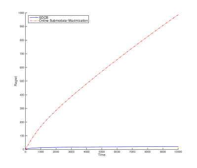
(a) Distribution 1

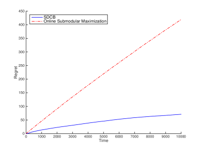
(b) Distribution 2

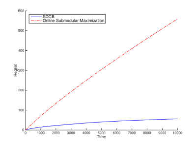
(c) Distribution 3

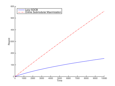
(d) Distribution 4

Figure 1: Regrets of SDCB/Lazy-SDCB and Algorithm 8 on the $K$-MAX problem, for distributions 1-4. The regrets are averaged over $20$ independent runs.

References

- [1] Jean-Yves Audibert and Sébastien Bubeck. Minimax policies for adversarial and stochastic bandits. In COLT, pages 217–226, 2009.
- [2] Peter Auer, Nicolo Cesa-Bianchi, and Paul Fischer. Finite-time analysis of the multiarmed bandit problem. Machine learning, 47(2-3):235–256, 2002.
- [3] Peter Auer, Nicolo Cesa-Bianchi, Yoav Freund, and Robert E. Schapire. The nonstochastic multiarmed bandit problem. SIAM Journal on Computing, 32(1):48–77, 2002.
- [4] Anand Bhalgat and Sanjeev Khanna. A utility equivalence theorem for concave functions. In IPCO, pages 126–137. Springer, 2014.
- [5] Sébastien Bubeck and Nicolò Cesa-Bianchi. Regret analysis of stochastic and nonstochastic multi-armed bandit problems. Foundations and Trends in Machine Learning, 5(1):1–122, 2012.
- [6] Nicolo Cesa-Bianchi and Gábor Lugosi. Combinatorial bandits. Journal of Computer and System Sciences, 78(5):1404–1422, 2012.
- [7] Shouyuan Chen, Tian Lin, Irwin King, Michael R. Lyu, and Wei Chen. Combinatorial pure exploration of multi-armed bandits. In NIPS, 2014.
- [8] Wei Chen, Yajun Wang, Yang Yuan, and Qinshi Wang. Combinatorial multi-armed bandit and its extension to probabilistically triggered arms. Journal of Machine Learning Research, 17(50):1–33, 2016.
- [9] Richard Combes, M. Sadegh Talebi, Alexandre Proutiere, and Marc Lelarge. Combinatorial bandits revisited. In NIPS, 2015.
- [10] Aryeh Dvoretzky, Jack Kiefer, and Jacob Wolfowitz. Asymptotic minimax character of the sample distribution function and of the classical multinomial estimator. The Annals of Mathematical Statistics, pages 642–669, 1956.
- [11] P. C. Fishburn. The foundations of expected utility. Dordrecht: Reidel, 1982.
- [12] Yi Gai, Bhaskar Krishnamachari, and Rahul Jain. Combinatorial network optimization with unknown variables: Multi-armed bandits with linear rewards and individual observations. IEEE/ACM Transactions on Networking, 20(5):1466–1478, 2012.
- [13] Ashish Goel, Sudipto Guha, and Kamesh Munagala. Asking the right questions: Model-driven optimization using probes. In PODS, pages 203–212. ACM, 2006.
- [14] Ashish Goel, Sudipto Guha, and Kamesh Munagala. How to probe for an extreme value. ACM Transactions on Algorithms (TALG), 7(1):12:1–12:20, 2010.
- [15] Aditya Gopalan, Shie Mannor, and Yishay mansour. Thompson sampling for complex online problems. In ICML, pages 100–108, 2014.
- [16] Branislav Kveton, Zheng Wen, Azin Ashkan, Hoda Eydgahi, and Brian Eriksson. Matroid bandits: Fast combinatorial optimization with learning. In UAI, pages 420–429, 2014.
- [17] Branislav Kveton, Zheng Wen, Azin Ashkan, and Csaba Szepesvári. Combinatorial cascading bandits. In NIPS, 2015.
- [18] Branislav Kveton, Zheng Wen, Azin Ashkan, and Csaba Szepesvári. Tight regret bounds for stochastic combinatorial semi-bandits. In AISTATS, pages 535–543, 2015.
- [19] Tze Leung Lai and Herbert Robbins. Asymptotically efficient adaptive allocation rules. Advances in applied mathematics, 6(1):4–22, 1985.
- [20] Jian Li and Amol Deshpande. Maximizing expected utility for stochastic combinatorial optimization problems. In FOCS, pages 797–806, 2011.
- [21] Jian Li and Wen Yuan. Stochastic combinatorial optimization via poisson approximation. In STOC, pages 971–980, 2013.
- [22] Tian Lin, Bruno Abrahao, Robert Kleinberg, John Lui, and Wei Chen. Combinatorial partial monitoring game with linear feedback and its applications. In ICML, pages 901–909, 2014.
- [23] Tian Lin, Jian Li, and Wei Chen. Stochastic online greedy learning with semi-bandit feedbacks. In NIPS, 2015.
- [24] Pascal Massart. The tight constant in the dvoretzky-kiefer-wolfowitz inequality. The Annals of Probability, pages 1269–1283, 1990.
- [25] George L. Nemhauser, Laurence A. Wolsey, and Marshall L. Fisher. An analysis of approximations for maximizing submodular set functions – I. Mathematical Programming, 14(1):265–294, 1978.
- [26] Matthew Streeter and Daniel Golovin. An online algorithm for maximizing submodular functions. In NIPS, 2008.
- [27] Jiajin Yu and Shabbir Ahmed. Maximizing expected utility over a knapsack constraint. Operations Research Letters, 44(2):180–185, 2016.