The Broadband Spectral Variability of Holmberg IX X-1

Abstract

We present results from four new broadband X-ray observations of the extreme ultraluminous X-ray source Holmberg IX X-1 ($L_{\rm{X}}>10^{40}$ erg s^-1), performed by Suzaku and NuSTAR in coordination. Combined with the archival data, we now have broadband observations of this remarkable source from six separate epochs. Two of these new observations probe lower fluxes than seen previously, allowing us to extend our knowledge of the broadband spectral variability exhibited. The spectra are well fit by two thermal blackbody components, which dominate the emission below 10 keV, as well as a steep ($\Gamma\sim 3.5$) powerlaw tail which dominates above $\sim$15 keV. Remarkably, while the 0.3–10.0 keV flux varies by a factor of $\sim$3 between all these epochs, the 15–40 keV flux varies by only $\sim$20%. Although the spectral variability is strongest in the $\sim$1–10 keV band, both of the thermal components are required to vary when all epochs are considered. We also re-visit the search for iron absorption features, leveraging the high-energy NuSTAR data to improve our sensitivity to extreme velocity outflows in light of the ultra-fast outflow recently detected in NGC 1313 X-1. Iron absorption from a similar outflow along our line of sight can be ruled out in this case. We discuss these results in the context of super-Eddington accretion models that invoke a funnel-like geometry for the inner flow, and propose a scenario in which we have an almost face-on view of a funnel that expands to larger radii with increasing flux, resulting in an increasing degree of geometrical collimation for the emission from intermediate temperature regions.

1. Introduction

Holmberg IX X-1 is one of the best studied members of the ultraluminous X-ray source (ULX) population (see Feng & Soria 2011 for a recent review on ULXs), as it is one of the few sources within $\sim$5 Mpc to persistently radiate at an extreme X-ray luminosity of $L_{\rm X}>10^{40}$ erg s^-1 (e.g. Kong et al. 2010; Vierdayanti et al. 2010; Walton et al. 2011; the distance to Holmberg IX is 3.55 Mpc, Paturel et al. 2002). Early observations of Holmberg IX X-1 with XMM-Newton (Jansen et al. 2001) suggested the presence of a cool accretion disk ($T_{\rm{in}}\sim 0.3$ keV; Miller et al. 2003, 2013), and a hard powerlaw continuum at higher energies ($>$2 keV), consistent with the expectation for low-Eddington rate accretion. This suggested the presence of a massive ($>$100 $\rm M_{\odot}$) black hole accreting from a standard thin disk. However, higher quality data subsequently revealed deviations from a powerlaw continuum in the $\sim$2–10 keV band (e.g. Stobbart et al. 2006; Gladstone et al. 2009; Walton et al. 2013b), calling this identification into question.

Most recently, our coordinated broadband observations of Holmberg IX X-1 with XMM-Newton, Suzaku (Mitsuda et al. 2007) and NuSTAR (Harrison et al. 2013) robustly confirmed that the X-ray continuum above $\sim$2 keV does not have a powerlaw form, in good agreement with the weak hard X-ray detection revealed by INTEGRAL  (Sazonov et al. 2014). Instead, the hard X-ray spectrum appears to be dominated by a second, hotter ($T\sim 3$ keV, at least at lower fluxes) multi-color blackbody emission component likely associated with the inner accretion disk, similar to the rest of the ULX population observed by NuSTAR to date (e.g. Bachetti et al. 2013; Walton et al. 2013a, 2015a, 2015b; Rana et al. 2015; Mukherjee et al. 2015), with a steep powerlaw tail also potentially detected at the highest energies (Walton et al. 2014). The broadband spectra observed are generally consistent with the expectation for super-Eddington accretion onto a compact stellar remnant (e.g. Shakura & Sunyaev 1973; Dotan & Shaviv 2011). Indeed, we now know that at least three of this population of extreme ULXs are actually highly super-Eddington neutron stars (Bachetti et al. 2014; Fürst et al. 2016; Israel et al. 2016, 2017). Furthermore, in the case of NGC 1313 X-1, another $L_{\rm X}\sim 10^{40}$ erg s^-1 ULX, discrete absorption features from a massive outflow have now finally been detected (Pinto et al. 2016b; Walton et al. 2016b), following an initial suggestion that low-energy ($\sim$1 keV) residuals could be related to such a wind (Middleton et al. 2014, 2015b). Large outflows from the accretion flow are broadly expected from super-Eddington accretion theory (e.g. Poutanen et al. 2007).

The most remarkable aspect of these broadband observations, however, is the unusual spectral variability. In our initial program, we obtained data from two epochs separated by $\sim$2 weeks. During the second epoch, Holmberg IX X-1 was significantly brighter than during the first by a factor of $\sim$2. This was primarily driven by an increase in the $\sim$1–15 keV bandpass, while the fluxes below $\sim$1 keV and above $\sim$15 keV remained relatively constant, resulting in a significantly more peaked spectrum in the second observation (Walton et al. 2014). The similar fluxes at the highest and lowest energies of the observed 0.3–40 keV bandpass implies that the variability is dominated by one of the two multi-color blackbody components, but with only two epochs it was not clear which; in either case, the observed evolution would be highly non-standard behavior for blackbody emission.

In order to further investigate the spectral variability exhibited by Holmberg IX X-1, we obtained four additional epochs of coordinated broadband observations with Suzaku and NuSTAR. Here, we present the results obtained with these new observations (hereafter epochs 3–6), along with a re-analysis of the archival data (epochs 1–2). This paper is structured as follows: section 2 describes our data reduction procedure, and section 3 describes our spectral analysis of the existing broadband datasets (both new and archival). Finally, we discuss our results and present our conclusions in section 4.

2. Observations and Data Reduction

Table 1 provides the details of the X-ray observations of Holmberg IX X-1 presented in this work. Our data reduction largely follows the procedures outlined in Walton et al. (2014). The XMM-Newton data for epochs 1 and 2 were re-reduced using SAS v14.0.0 in exactly the same manner as described in our previous work for both the EPIC-pn and EPIC-MOS detectors (Strüder et al. 2001; Turner et al. 2001), using more recent calibration files (up-to-date as of July 2015). Our new Suzaku observations (epochs 3–6) were also reduced with HEASOFT v6.18 in the same manner as the epoch 1 data; as before we only utilize the XIS detectors (Koyama et al. 2007) given the high-energy NuSTAR coverage. The only major update to our data reduction procedure in comparison to Walton et al. (2014) is for the NuSTAR data. The standard science data (mode 1) were reduced with NUSTARDAS v1.5.1 in the same manner as in that work, again with updated calibration files (NuSTAR CALDB 20150316). However, in order to maximize the S/N, in this work we also make use of the spacecraft science data (mode 6) following the procedure outlined in Walton et al. (2016c, see also the NuSTAR Users Guide). In brief, spacecraft science mode refers to data recorded during periods of the observation in which the X-ray source is still visible, but the star tracker on the optics bench cannot return a good aspect solution. During such times, the star trackers on the spacecraft bus are utilized instead. For these observations, this provides an additional $\sim$20–40% good exposure (depending on the observation). The inclusion of the mode 6 data allows us to fit the NuSTAR data for Holmberg IX X-1 from 3 to 40 keV for all epochs. As in Walton et al. (2014), we model the XMM-Newton spectra over the 0.3–10.0 keV range, and the Suzaku data over the 0.6–10.0 keV range for the front-illuminated XIS units (XIS0, XIS3) and the 0.7–9.0 keV range for the back-illuminated XIS1, excluding 1.7–2.1 keV owing to known calibration issues around the instrumental edges.

Table 1Details of the X-ray observations of Holmberg IX X-1 considered in this work, ordered chronologically.

Mission	OBSID	Date	Good Exposure[a]
			(ks)
Epoch 1 (medium flux)
Suzaku	707019020	2012-10-21	107
XMM-Newton	0693850801	2012-10-23	6/10
Suzaku	707019030	2012-10-24	107
XMM-Newton	0693850901	2012-10-25	7/13
Suzaku	707019040	2012-10-26	110
NuSTAR	30002033002	2012-10-26	43 (12)
NuSTAR	30002033003	2012-10-26	124 (36)
XMM-Newton	0693851001	2012-10-27	4/13
Epoch 2 (high flux)
NuSTAR	30002033005	2012-11-11	49 (8)
NuSTAR	30002033006	2012-11-11	41 (6)
XMM-Newton	0693851701	2012-11-12	7/9
NuSTAR	30002033008	2012-11-14	18 (3)
XMM-Newton	0693851801	2012-11-14	7/9
NuSTAR	30002033010	2012-11-15	59 (10)
XMM-Newton	0693851101	2012-11-16	3/7
Epoch 3 (medium flux)
NuSTAR	30002034002	2014-05-02	82 (24)
Suzaku	707019010	2014-05-03	32
Epoch 4 (low flux)
NuSTAR	30002034004	2014-11-15	81 (20)
Suzaku	707019020	2014-11-15	34
Epoch 5 (low flux)
NuSTAR	30002034006	2015-04-06	64 (14)
Suzaku	707019030	2015-04-06	32
Epoch 6 (medium flux)
NuSTAR	30002034008	2015-05-16	67 (10)
Suzaku	707019040	2015-05-16	34

^a XMM-Newton exposures are listed for the EPIC-pn/MOS detectors, while the NuSTAR exposures quoted are the total for each of the focal plane modules, with the mode 6 contribution in parentheses, and the Suzaku exposures quoted are for each of the operational XIS units.

In the following sections, we perform spectral analysis with XSPEC  v12.6.0f (Arnaud 1996), and quote parameter uncertainties at the 90% confidence level for one interesting parameter. Cross-calibration uncertainties between the different detectors are accounted for by allowing multiplicative constants to float between the datasets from a given epoch, fixing FPMA at unity. The values are within $\sim$10% (or less) of unity, as expected (Madsen et al. 2015).

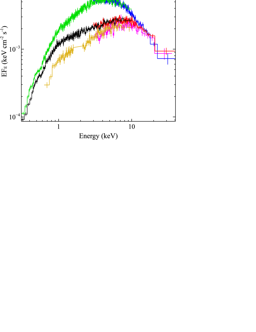
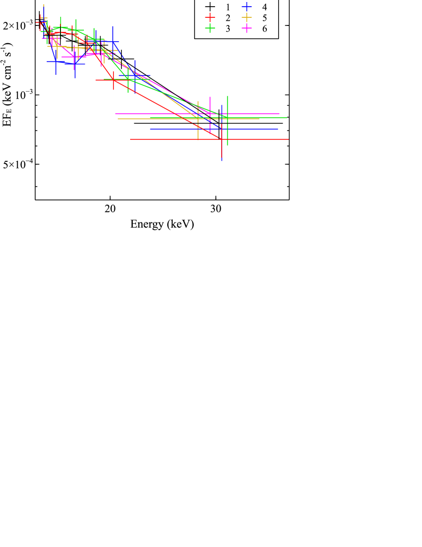
Figure 1.— Left: The broadband spectral evolution displayed by Holmberg IX X-1. We show the data from epochs 1, 2 and 4, being representative of the three ‘states’ (medium, high and low, respectively) now covered with broadband X-ray observations. For clarity, we only show the NuSTAR data from FPMA (red, blue and magenta for epochs 1, 2 and 4, respectively) along with one of the accompanying soft X-ray detectors (black, green and orange for epochs 1, 2 and 4, respectively, with epochs 1 and 2 showing data from EPIC-pn on XMM-Newton, and epoch 4 showing the FI XIS units on Suzaku). Of the three other new broadband epochs presented in this work, two are similar to epoch 1 (epochs 3 and 6) and the other (epoch 5) is similar to epoch 4. Right: The high-energy ($>$15 keV) data from NuSTAR (again, FPMA only for clarity). Here we show the data from all six epochs, demonstrating the relative lack of variability observed above $\sim$15 keV in comparison to the lower energy data. All the data have been unfolded through the same model, which is simply constant with energy, and the data have been further rebinned for visual purposes.

3. Spectral Analysis

The primary goal of our follow-up Suzaku+NuSTAR observations was to obtain broadband observations of Holmberg IX X-1 in flux states that differ from those presented in Walton et al. (2014), such that we can improve our understanding of the unusual broadband spectral variability exhibited by this source. Of the additional four epochs we obtained, the first (epoch 3) was found to be extremely similar to the fainter of the two states observed in our original observations (epoch 1). The following two (epochs 4 and 5) were also very similar to each other, but distinct from epochs 1–3, probing even lower fluxes. Finally, the last (epoch 6) was again broadly similar to epochs 1 and 3, although epoch 6 is slightly fainter overall and so is not completely identical.

Throughout this work, we group the observations into low (epochs 4 and 5), medium (epochs 1, 3 and 6) and high (epoch 2) states, as indicated in Table 1. The broadband spectrum from epoch 4 is shown in comparison to epochs 1 and 2 in Figure 1 (left panel). The evolution from the flux exhibited in epoch 1 to the even lower fluxes observed during epochs 4 and 5 is primarily dominated by variability at low energies. Remarkably, the high-energy data appears to remain extremely similar for all six epochs probed by NuSTAR to date, as also shown in Figure 1 (right panel). Indeed, if we fit the 15–40 keV NuSTAR data for all the epochs with a simple powerlaw model, we find that the photon indices are all consistent within their $\sim$90% confidence limits ($\Gamma\sim 3.5$), and the 15–40 keV fluxes only vary by $\sim$20%, despite the factor of $>$2 differences seen below 10 keV (Walton et al. 2014).

3.1. Broadband Spectral Variability

In order to characterize the spectra and study the observed spectral variability, we fit each of the six epochs with a common model, such that the results from each can be directly compared. In order to obtain the tightest constraints, and determine which of the model parameters are important in producing the spectral variability, we analyse the broadband data from all six epochs simultaneously.

We focus on the model presented in Walton et al. (2014) that combines DISKBB, DISKPBB and SIMPL (Mitsuda et al. 1984; Mineshige et al. 1994; Steiner et al. 2009), which was able to successfully describe the first two broadband epochs. We refer the reader to Walton et al. (2014) for full details, but in brief the DISKBB and DISKPBB components account for the two thermal components that dominate the spectrum below $\sim$15 keV (the former assumes the thin disk model outlined in Shakura & Sunyaev 1973, while the latter allows for an accretion disk continuum with a variable radial temperature index), with SIMPL applied to the higher-temperature DISKPBB component to provide the high-energy powerlaw tail that is present above $\sim$15 keV. In addition to these continuum components, the model also includes two neutral absorption components, modeled with TBABS. We use the abundance set of Wilms et al. (2000) and the cross-sections of Verner et al. (1996). The first of these components is fixed at the Galactic column ($N_{\rm{H,Gal}}=5.54\times 10^{20}$ cm^-2; Kalberla et al. 2005), and the second is assumed to be intrinsic to either the Holmberg IX galaxy ($z=0.000153$) or to the Holmberg IX X-1 system itself.

Table 2Results obtained for the dual-thermal model combining the DISKBB and DISKPBB multicolor blackbody disk compoents for the six broadband epochs currently available for Holmberg IX X-1

Model	Parameter		Global	Epoch
Component				1	2	3	4	5	6
Constant DISKBB temperature
TBABS	$N_{\rm{H,int}}$	[$10^{21}$ cm-2]	$1.45\pm 0.08$
DISKBB	$T_{\rm{in}}$	[keV]	$0.29\pm 0.02$
	Norm			$11^{+3}_{-2}$	$14^{+6}_{-4}$	$17^{+6}_{-4}$	$11^{+4}_{-3}$	$11\pm 3$	$4^{+3}_{-2}$
DISKPBB	$T_{\rm{in}}$	[keV]		$2.6^{+0.4}_{-0.1}$	$1.3^{+0.9}_{-0.1}$	$2.6^{+0.3}_{-0.2}$	$2.6^{+0.4}_{-0.1}$	$2.6^{+0.3}_{-0.2}$	$2.9^{+0.3}_{-0.2}$
	$p$			$0.574^{+0.005}_{-0.004}$	$0.69^{+0.03}_{-0.02}$	$0.60\pm 0.01$	$0.63^{+0.01}_{-0.02}$	$0.64^{+0.02}_{-0.01}$	$0.56\pm 0.01$
	Norm	[$10^{-3}$]		$3.2^{+0.6}_{-1.1}$	$190^{+70}_{-80}$	$3.8^{+1.4}_{-1.5}$	$3.5^{+1.2}_{-1.4}$	$4.2^{+1.6}_{-1.7}$	$1.8\pm 0.7$
SIMPL	$\Gamma$		$3.68^{+0.07}_{-0.05}$
	$f_{\rm{scat}}$	[%]	$>67$
$\chi^{2}$/DoF			8792/8515
Constant DISKPBB temperature
TBABS	$N_{\rm{H,int}}$	[$10^{21}$ cm-2]	$1.50\pm 0.07$
DISKBB	$T_{\rm{in}}$	[keV]		$0.28^{+0.02}_{-0.01}$	$1.70^{+0.04}_{-0.03}$	$0.26\pm 0.02$	$0.30\pm 0.03$	$0.29\pm 0.03$	$0.41\pm 0.06$
	Norm			$12^{+4}_{-3}$	$0.063\pm 0.005$	$27^{+15}_{-9}$	$10^{+5}_{-3}$	$10^{+6}_{-4}$	$2.2^{+1.8}_{-0.9}$
DISKPBB	$T_{\rm{in}}$	[keV]	$2.9^{+0.4}_{-1.1}$
	$p$			$0.571\pm 0.004$	$0.542\pm 0.005$	$0.59\pm 0.01$	$0.63^{+0.01}_{-0.02}$	$0.63\pm 0.01$	$0.58\pm 0.01$
	Norm	[$10^{-3}$]		$2.3\pm 0.9$	$1.7^{+0.6}_{-0.7}$	$2.5^{+1.1}_{-0.8}$	$2.6^{+1.3}_{-0.9}$	$2.7^{+1.3}_{-1.0}$	$2.1^{+1.0}_{-0.9}$
SIMPL	$\Gamma$		$>3.4$[a]
	$f_{\rm{scat}}$	[%]	$>41$
$\chi^{2}$/DoF			8789/8515
$F_{0.3-40.0}$[b]	[$10^{-12}$ $\rm\thinspace erg~{}cm^{-2}~{}s^{-1}$]			$12.8^{+0.2}_{-0.1}$	$22.3\pm 0.2$	$12.4\pm 0.2$	$10.1\pm 0.2$	$9.8\pm 0.2$	$11.5\pm 0.2$
$F_{0.3-1.0}$[b]				$1.02\pm 0.02$	$1.47\pm 0.02$	$1.01\pm 0.03$	$0.66\pm 0.03$	$0.60\pm 0.03$	$0.87\pm 0.03$
$F_{1.0-10.0}$[b]				$8.6\pm 0.1$	$17.5\pm 0.2$	$8.2\pm 0.2$	$6.6\pm 0.1$	$6.3\pm 0.1$	$7.8\pm 0.2$
$F_{10.0-40.0}$[b]				$3.23\pm 0.08$	$3.17\pm 0.09$	$3.29\pm 0.12$	$3.01\pm 0.12$	$2.91\pm 0.12$	$3.07\pm 0.13$
$L_{0.3-40.0}$[c]	[$10^{40}$ erg s-1]			$2.30\pm 0.03$	$3.84\pm 0.05$	$2.23\pm 0.05$	$1.77\pm 0.04$	$1.68\pm 0.04$	$2.08\pm 0.05$

^a We set an upper limit for the photon index of $\Gamma\leq 4.0$.
^b The observed flux in the full 0.3–40.0 keV band, and the 0.3–2.0, 2.0–10.0 and 10.0–40.0 keV sub-bands, respectively (consistent for both models).
^c De-absorbed luminosity in the full 0.3–40.0 keV band. These values assume isotropic emission, and may therefore represent upper limits (see Section 4).

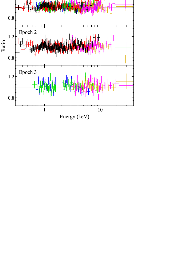
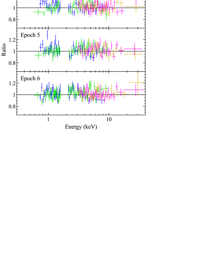
Figure 2.— Data/model ratios for the constant DISKPBB temperature model presented in Table 2. EPIC-pn, EPIC-MOS, FI XIS, BI XIS, FPMA and FPMB data are shown in black, red, green, blue, magenta and orange, respectively, and the data have been further rebinned for visual purposes.

As a starting point, we apply our model with the high-energy photon index of the SIMPL component and the neutral absorption column intrinsic to Holmberg IX linked between the different epochs (but still free to vary globally). We link the former following our analysis of the 15–40 keV spectrum above, while we link the latter because for the two broadband epochs with XMM-Newton coverage down to 0.3 keV (epochs 1 and 2) we found the neutral absorption column to be consistent in our prior work on these data (see also Miller et al. 2013, who find that a constant column provides a good fit to all the archival XMM-Newton observations of Holmberg IX X-1), and the remaining epochs only have coverage down to 0.7 keV, reducing their sensitivity to small variations in $N_{\rm H}$. Following Walton et al. (2014), we restrict the range over which the photon index can vary to be $1.5\leq\Gamma\leq 4.0$. The parameters that are initially allowed to vary from epoch to epoch are therefore the inner temperatures ($T_{\rm{in}}$) and normalizations of the DISKBB and DISKPBB components, the radial temperature index ($p$) of the DISKPBB component, and the scattered fraction ($f_{\rm{scat}}$) for the SIMPL component, which acts as an effective normalization for the high-energy powerlaw tail. This model provides a good global fit to the six available broadband epochs: $\chi^{2}$ = 8779 for 8505 degrees of freedom (DoF).

From this baseline, we proceed to investigate which of the other key model parameters drive the observed variability by trying to link them across each of the epochs (but again allowing them to vary globally), beginning with the temperatures of each of the DISKBB and DISKPBB components in turn. Neither of these scenarios significantly degrades the quality of the fit, and we find that both provide very similar fits, with a constant temperature for the hotter DISKPBB component marginally preferred: fixing the DISKBB temperature results in a fit of $\chi^{2}$/DoF = 8792/8510 (worse by $\Delta\chi^{2}=13$ for 5 fewer free parameters), and fixing the DISKPBB temperature results in a fit of $\chi^{2}$/DoF = 8786/8510 (worse by $\Delta\chi^{2}=7$, also for 5 fewer free parameters). However, if we try to fix both of the temperatures across all epochs, the global fit does worsen significantly, resulting in $\chi^{2}$/DoF = 8931/8515. This is because, as discussed in Walton et al. (2014), with this simple parameterization the temperature of one of the two thermal components must evolve to explain the observed differences between epochs 1 and 2.

Next we consider the radial temperature index for the DISKPBB component. Regardless of which of the DISKBB or DISKPBB temperatures we choose to link, additionally linking $p$ significantly worsens the fit. With a constant temperature for the cooler DISKBB component, the fit degrades to $\chi^{2}$/DoF = 8952/8515 ($\Delta\chi^{2}$ = 160, 5 fewer free parameters), and with a constant temperature for the hotter DISKPBB component the fit degrades to $\chi^{2}$/DoF = 8890/8515 ($\Delta\chi^{2}$ = 104). This is also the case if we do not link either of the temperatures at all, in which case the best fit is $\chi^{2}$/DoF = 8850/8510 ($\Delta\chi^{2}$ = 71, compared to the fit with both temperatures free), so the observed variation in $p$ is not merely a consequence of this choice. The radial temperature index $p$ determines the slope of the DISKPBB model up to the point at which it falls away with a Wien spectrum (set by $T_{\rm{in}}$). This is critical in determining the slope of the observed spectrum in the $\sim$1–7 keV energy range for the lower flux states, given the low temperatures ($\sim$0.3 keV) obtained for the DISKBB component. Therefore, even if one tries to assign the majority of the variability to the lower temperature DISKBB component by requiring that the DISKPBB temperature is constant, the spectral form of the this hotter component is still required to vary. While the values vary, we consistently find that $p<0.75$ (the value expected for a thin disk; Shakura & Sunyaev 1973), which would suggest a disk in which photon advection is important (e.g. Abramowicz et al. 1988).

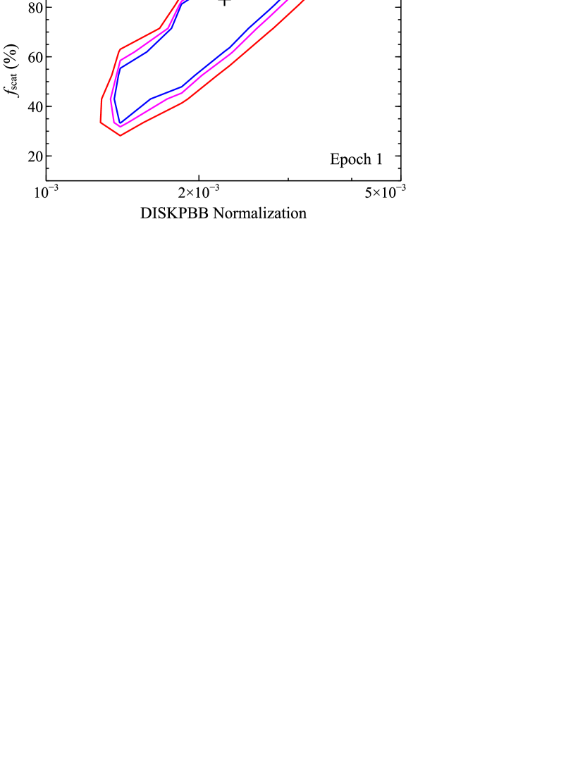
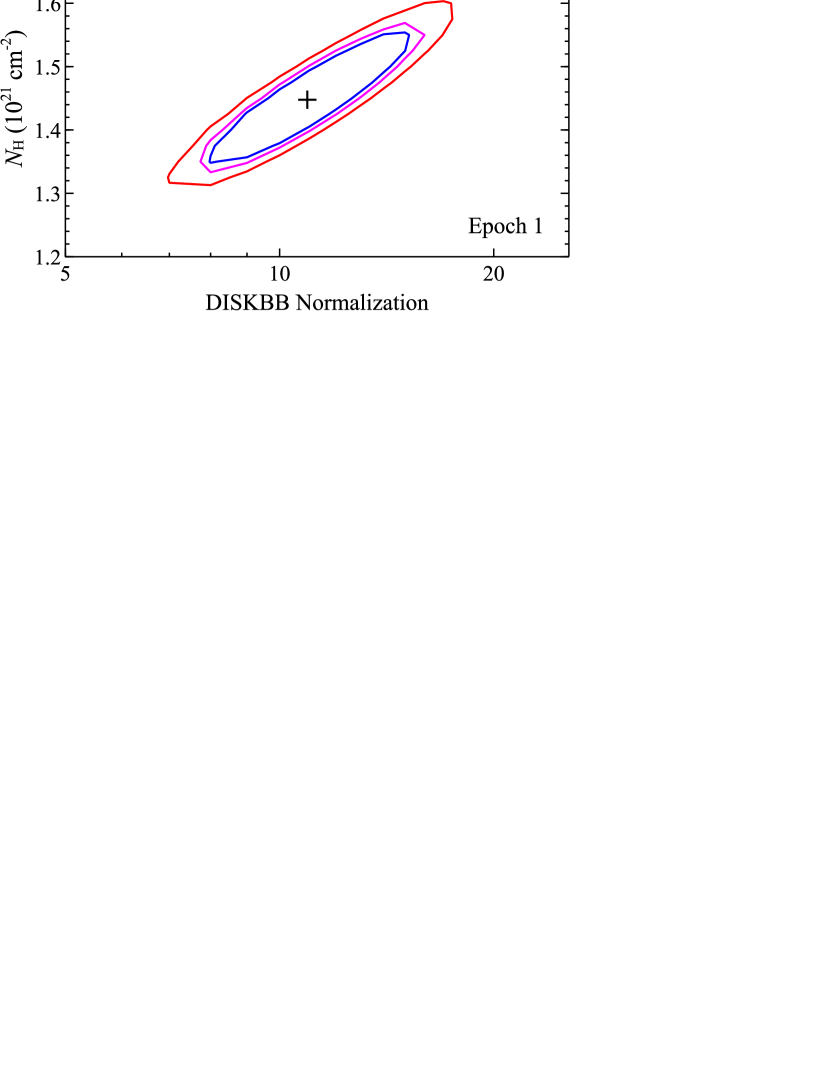
Figure 3.— Top panel: 2D confidence contours for the DISKPBB normalization from epoch 1 and $f_{\rm{scat}}$ calculated for the scenario with a constant DISKPBB temperature, showing an example of the general degeneracy between these parameters that is seen for all epochs. The 90, 95 and 99% confidence contours for two parameters of interest are shown in blue, magenta and red, respectively. Bottom panel: An example of the similar degeneracy seen between the DISKBB normalization from epoch 1 and $N_{\rm H}$ for the scenario in which the DISKBB temperature is constant.

Throughout all these fits, we find that in addition to the photon index we can also link the scattered fraction for the SIMPL component across all the epochs. With a constant temperature for the cooler DISKBB component, additionally linking $f_{\rm{scat}}$ gives a fit of $\chi^{2}$/DoF = 8795/8515, and doing so with a constant temperature for the hotter DISKPBB component gives a fit of $\chi^{2}$/DoF = 8789/8515 (i.e. $\Delta\chi^{2}$ = 3 for another 5 fewer free parameters in both cases). The best-fit parameters for these two scenarios are given in Table 2, and data/model ratio plots for the constant DISKPBB temperature scenario are shown for all six epochs in Figure 2. Although in this scenario the normalizations for the DISKPBB component also appear to be consistent with remaining constant, this is related to a significant degeneracy between these normalizations and $f_{\rm{scat}}$ (see Figure 3); trying to link this parameter across all epochs results in a significant degradation in the quality of fit ($\Delta\chi^{2}=135$ for another 5 fewer free parameters). SIMPL is a convolution model and $f_{\rm{scat}}$ indicates the fraction of the input model scattered into the high-energy continuum, so with our parameterization this acts as a normalization for this continuum relative to the DISKPBB component. As $f_{\rm{scat}}$ is linked across all epochs, changing this parameter therefore causes each of the DISKPBB normalizations to change in tandem (i.e. increasing $f_{\rm{scat}}$ causes all of the DISKPBB normalizations to increase together). This degeneracy therefore expands the formal uncertainties on each of the normalizations, but does not remove the need for the relative variations between epochs seen in the best-fit values.

There is a similar issue between the DISKBB normalizations and the neutral absorption column density in the scenario in which the DISKBB temperature is constant. There is a degeneracy between these parameters for all epochs (again, see Figure 3), and as $N_{\rm H}$ is linked between them changing this parameter again causes all of the DISKBB normalizations to vary in tandem, such that the relative differences indicated by the best-fit values in Table 2 remain. Both the thermal components are therefore required to change in at least their normalizations in both scenarios; the observed spectral variability between these six broadband epochs cannot be explained by variations in one of these model components only.

Finally, we stress that with the additional data included in this work, the requirement for the high-energy powerlaw tail is highly significant for any continuum model that falls away as a Wien tail. If we remove the SIMPL component and then allow the temperatures of both of the two thermal components to vary between epochs, we find a fit of $\chi^{2}$/DoF = 8875/8512 with clear excesses of emission seen in the residuals above $\sim$20 keV. This is worse by $\Delta\chi^{2}>80$ despite there being three additional free parameters in comparison to either of the fits presented in Table 2. Furthermore, this is also the case if we replace the hotter DISKPBB with a thermal Comptonization component (COMPTT; Titarchuk 1994), another model that is frequenly considered in the literature.

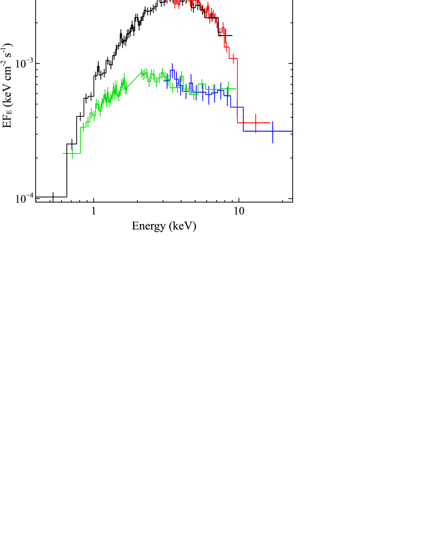
Figure 4.— The broadband difference spectra computed in Section 3.2. For clarity, we only show the EPIC-pn and FPMB data for the “high–med” difference spectrum (black and red, respectively), and the FI XIS and FPMB data for the “med–low” difference spectrum (green and blue, respectively). The two difference spectra are clearly distinct from each other. As with Figure 1, all the data have been unfolded through a model that is constant with energy, and have been further rebinned for visual purposes.

3.2. Difference Spectroscopy

In order to further probe the spectral variability observed, we also compute ‘difference spectra’ between the three different flux states probed with broadband observations to date. This involves using a lower flux source spectrum as the background for a higher flux observation, allowing us to isolate the additional emission in the latter in a model-independent manner. Given the instrumental differences, only spectra obtained with the same detectors can be meaningfully subtracted from one another. While NuSTAR coverage is common among all these epochs, with respect to the soft X-ray coverage the high and medium flux states only have XMM-Newton coverage in common, while the medium and low flux states only have the Suzaku coverage in common.

In order to compute a broadband difference spectrum between the high and medium states, we therefore use the XMM-Newton and NuSTAR data from epoch 1 as the background for epoch 2; owing to the different pattern selections for the EPIC-MOS data between epochs 1 and 2 to avoid pile-up during epoch 2 (as discussed in Walton et al. 2014), we only consider the EPIC-pn data for XMM-Newton here. For the difference spectrum between the medium and low states, given that the new observations (epochs 3–6) each have significantly shorter exposures than epochs 1 and 2, we first co-added the Suzaku and NuSTAR data from epochs 4 and 5, and then used these spectra as the background for epoch 1. Given that the spectra from different epochs are often quite similar, particularly towards the highest and lowest energies covered here, we substantially increase the bininng of the data to a minimum of 1000 counts per bin to ensure that the data in the difference spectra are of sufficient S/N to use $\chi^{2}$ minimization. Unfortunately there is no common soft X-ray instrumental coverage between the high and low states, so we are not able to compute a broadband difference spectrum in this case.

The two broadband difference spectra are shown in Figure 4. Clearly, the two difference spectra have distinct spectral forms. The “high–med” (hereafter HM) difference spectrum is very strongly peaked at $\sim$4 keV, which is not surprising given that the epoch 1 and 2 spectra are very similar below $\sim$1 keV, and all the spectra are very similar above $\sim$15 keV. In contrast, the “med–low” (hereafter ML) difference spectrum has a much broader profile, but also falls away at the highest and lowest energies. In order to characterize and further investigate the differences between them, we proceed to fit these difference spectra with a variety of simple continuum models. All models also include a neutral absorber (modeled again with TBABS) at the redshift of Holmberg IX X-1, but we do not include Galactic absorption as this should remain constant with time.

We start with the HM difference spectrum. Unsurprisingly, given the strong curvature, a powerlaw continuum provides an extremely poor fit to the data ($\chi^{2}$/DoF = 1820/148). Instead, an accretion disk continuum (DISKBB) provides a good fit ($\chi^{2}$/DoF = 173/148), capturing this curvature rather well. We also test the DISKPBB model, allowing the radial temperature index to be a free parameter, and find a moderate improvement over the DISKBB case ($\chi^{2}$/DoF = 161/147). However, in contrast to the DISKPBB results for the actual spectra, here we find $p>0.75$, implying the emission is slightly more peaked than a standard thin disk continuum. A run of blackbody temperatures is still required though, as a single temperature blackbody continuum provides a very poor fit to the data ($\chi^{2}$/DoF = 706/148).

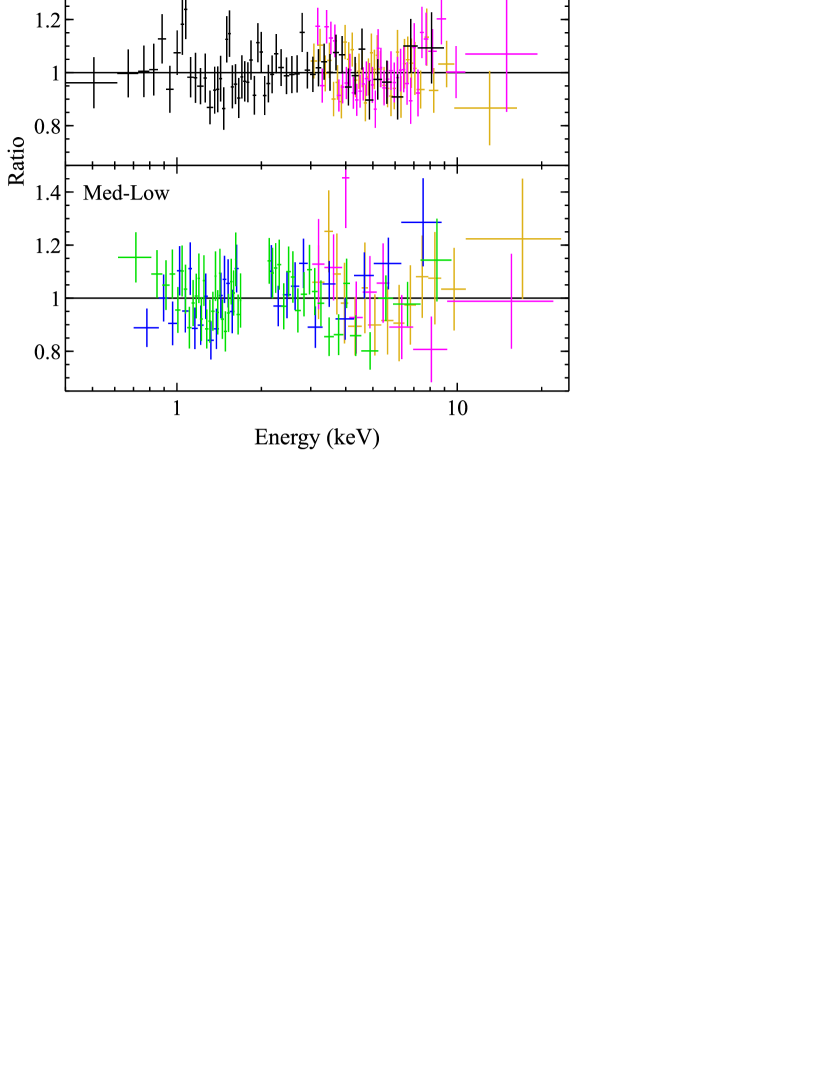
Figure 5.— Data/model ratios for the two difference spectra considered in Section 3.2 fit with the DISKPBB model. The color coding is the same as Figure 2 and again the data have been further rebinned for visual purposes.

Table 3Results obtained modeling the difference spectra with a simple DISKPBB continuum

Parameter		High–Med	Med–Low
$N_{\rm{H,int}}$	[$10^{21}$ cm-2]	$2.1^{+0.5}_{-0.4}$	$3.6\pm 0.5$
$T_{\rm{in}}$	[keV]	$1.52^{+0.03}_{-0.04}$	$2.9^{+0.5}_{-0.3}$
$p$		$0.87^{+0.08}_{-0.06}$	$0.50\pm 0.01$
Norm		$0.14^{+0.04}_{-0.03}$	$(5\pm 3)\times 10^{-4}$
$\chi^{2}$/DoF		161/147	490/423

For the ML difference spectrum, a powerlaw continuum provides a more acceptable fit than the HM case ($\chi^{2}$/DoF = 554/424), but still fails to capture the broad curvature seen in the data. Here, the DISKBB model also provides a poor fit ($\chi^{2}$/DoF = 720/424), with the spectral form being significantly less peaked than a standard thin disk continuum. The DISKPBB model again provides a good fit to the data though ($\chi^{2}$/DoF = 490/423), with the radial temperature index required to be significantly flatter than the thin disk case.

We provide the best-fit parameters for the DISKPBB model in Table 3 for direct comparison, and show the data/model ratios for these fits in Figure 5 as this is the only model to yield good fits for both difference spectra.. The results are clearly different for the two difference spectra. We have already highlighted the difference in the radial temperature index inferred, and the temperatures obtained are also very different. In addition, the results for the ML difference spectrum also differ significantly from the best-fit parameters for the DISKBB and DISKPBB spectral components for epoch 1 (for both the scenarios considered). While the temperature is similar to the hotter DISKPBB component, $p$ is significantly flatter. This provides further evidence that the energy and flux-dependent variability shows some complexity, and in the context of simple dual-thermal models cannot be explained by variations in only one of the spectral components required to model the observed data.

Finally, we note that the absorption columns obtained for the models that fit the data well are slightly larger than obtained fitting the actual observed spectra (for the HM difference spectrum, the column obtained with the DISKBB model is slightly higher again than for the DISKPBB model). However, given that the column is consistent with remaining constant for all epochs when modeling the actual spectra, this does not likely imply variable absorption (as may be seen, for example, in NGC 1313 X-1; Middleton et al. 2015b). Instead, this just indicates that the relative variations are weaker below $\sim$1 keV than in the $\sim$1–10 keV range, where the variability seen in both difference spectra peaks.

3.3. Fe K Line Search

Lastly, we also re-visit the limits on the presence of any atomic iron absorption or emission features in light of the ultra-fast outflow ($\sim$0.2–0.25$c$) recently detected in NGC 1313 X-1 (Pinto et al. 2016b; Walton et al. 2016b). The high-energy constraints provided by the NuSTAR data, missing in our previous line searches for Holmberg IX X-1 (Walton et al. 2012, 2013b), mean we can now significantly improve our sensitivity to any features associated with high-velocity outflows for this source. Considering the XMM-Newton, Suzaku and NuSTAR databases, the majority of the archival exposure available for Holmberg IX X-1 covers states similar to epoch 1, and so we focus on these data in order to maximize the S/N while considering only observations with similar spectra. Following Walton et al. (2016b), we also only consider XMM-Newton  observations in which Holmberg IX X-1 was placed on-axis in order to avoid increased background emission from copper lines at $\sim$8 keV seen in the EPIC-pn detector away from the optical axis (Carter & Read 2007), which fall in the energy range of interest. Therefore, in addition to the data from epochs 1, 3 and 6, we also include archival data from a further long Suzaku exposure (OBSID 707019010), and two short XMM-Newton exposures (ODSIDs 0112521001 and 0112521101). These are reduced in the same manner as the other XMM-Newton and Suzaku observations, and then the data are co-added to produce average spectra for each of the Suzaku FI and BI XIS detectors, the XMM-Newton EPIC-pn and EPIC-MOS detectors, and the NuSTAR FPMA and FPMB modules. The total good exposures utilized are 570 ks for each of the operational XIS units, 32 ks for the EPIC-pn detector, 56 ks for each of the EPIC-MOS detectors, and 315 ks for each FPM.

For this analysis, we focus on the 3.5–20.0 keV energy range and model the continuum local to the iron band with a simple CUTOFFPL model, as the spectral curvature in this bandpass is well established (Stobbart et al. 2006; Gladstone et al. 2009; Walton et al. 2013b, 2014). This bandpass is sufficient to accurately model the continuum local to the iron band; extending to lower energies we find that the fact that the 0.3–10 keV energy range requires two components starts to influence the high-energy continuum fit. We also include the two neutral absorption components included in our primary spectral analysis (Galactic and intrinsic to Holmberg IX), with the latter fixed to $N_{\rm{H,int}}=1.5\times 10^{21}$ cm^-2 based on the results above (see also Miller et al. 2013) since the bandpass considered is not particularly sensitive to this parameter. This provides an excellent fit to the 3.5–20.0 keV emission, with $\chi^{2}$/DoF = 2287/2269. The photon index and high-energy cutoff obtained are $\Gamma=1.07^{+0.04}_{-0.05}$ and $E_{\rm{cut}}=7.3\pm 0.3$ keV, and the model normalisation at 1 keV is $(1.22\pm 0.05)\times 10^{-3}$ $\rm\thinspace ct~{}keV^{-1}~{}cm^{-2}~{}s^{-1}$.

To search for atomic features, we follow a similar approach to our prior work on ULX outflows (e.g. Walton et al. 2013b, 2016b). The reader is referred to Walton et al. (2012) for more details, but in brief, we slide a narrow ($\sigma=10$ eV) Gaussian across the energy range of interest in steps of 40 eV (oversampling the Suzaku energy resolution by a factor $\sim$4). The Gaussian normalization is allowed to be either positive or negative (i.e. we allow for both emission and absorption, respectively), and for each line energy we record the $\Delta\chi^{2}$ improvement in the fit provided by the line, as well as the best-fit equivalent width ($\mathrm{EW}$) and its 90 and 99% confidence limits. These limits are calculated with the EQWIDTH command in XSPEC, using 10,000 simulated parameter combinations based on the best fit model parameters and their uncertainties. To be conservative, we vary the line energy between 6.0 and 10.0 keV, corresponding to a wide range of outflow velocities extending up to $\sim$0.3$c$ for Fe XXVI.

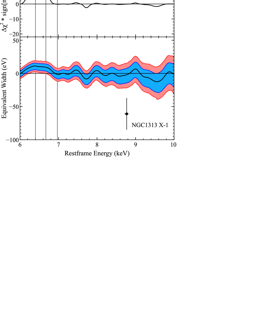
Figure 6.— Results from our search for narrow atomic iron features in the integrated spectra of observations similar to the ‘medium’ flux state seen in our broadband observations (epochs 1, 3 and 6; see Section 3.3). Top: the $\Delta$$\chi^{2}$ improvement provided by a narrow Gaussian line as a function of rest frame line energy. Positive values of $\Delta$$\chi^{2}$ indicate the improvement is obtained with an emission line, and negative values indicate absorption. There is a weak indication of excess emission conistent with neutral iron (the rest frame transitions of neutral, helium-like and hydrogen-like iron are shown with vertical dashed lines). However, we find no compelling evidence for any narrow absorption features, even with the additional sensitivity to extreme velocity outflows provided by the high-energy NuSTAR data. Bottom panel: 90% (blue) and 99% (red) confidence contours for the narrow line equivalent width, indicating for the majority of the bandpass considered the line strengths any narrow absorption features present in the data could have and still remain undetected. For context, we show the high-energy absorption feature detected in NGC 1313 X-1 (Walton et al. 2016b). Similar absorption along our line of sight to Holmberg IX X-1 can confidently be ruled out.

The results are shown in Figure 6. There is a weak indication of some iron emission, with a Gaussian emission line providing a moderate improvement over a range of energies in the immediate iron bandpass. To investigate this further, we perform additional fits modeling this excess emission first as a single Gaussian emission line with the energy, width and normalization all free to vary, and second with two narrow ($\sigma=10$ eV) emission lines with energies fixed at the K $\alpha$ transitions for Fe I and Fe XXV (6.4 and 6.67 keV, respectively), and find that both scenarios fit the data equally well. In the former scenario, the fit is improved by $\Delta\chi^{2}$/DoF = 18/3 and we find a line energy of $E=6.44^{+0.14}_{-0.13}$ keV, a line width of $\sigma=0.24^{+0.24}_{-0.11}$ keV and an equivalent width of $\mathrm{EW}=27\pm 14$ eV. In the latter, the fit is improved by by $\Delta\chi^{2}$/DoF = 16/2, and we find equivalent widths of $\mathrm{EW}_{\rm{FeI}}=11\pm 5$ and $\mathrm{EW}_{\rm{FeXXV}}=8^{+7}_{-6}$ eV, respectively.

Based on the well-established relation between the narrow Fe K equivalent width and the line-of-sight absorption observed in Galactic high-mass X-ray binaries, which is consistent with expectation for a spherical reprocessing geometry, for an absorption column of $N_{\rm{H}}=1.5\times 10^{21}$ $\rm\thinspace cm^{-2}$ we would expect an equivalent width of only $\sim$0.5 eV (Torrejón et al. 2010). This is significantly smaller than observed even in the case that the excess emission arises from both Fe I and Fe XXV, suggesting that the geometry of the reprocessing material cannot be spherical, and there must be additional reprocessing material out of our line-of-sight in this case. However, the observed equivalent widths are too small for the reprocessor to be the accretion disk (e.g. George & Fabian 1991), and the disk temperatures for super-Eddington accretion onto stellar remnant accretors should be too hot to produce Fe I emission, so the line emission likely has some other origin.

More importantly, we find no significant indication of any absorption features, even after extending our search out to cover extreme outflow velocities. Thanks to the high-energy coverage from NuSTAR, the limits on any narrow features present in the spectrum but undetected by these data remain tight right up to 10 keV, a significant improvement on our previous work (Walton et al. 2013b). The weakest limits, at $\sim$9.6 keV, require any undetected absorption features to have $\mathrm{EW}<40$ eV at 99% confidence, but the limits are more typically $\mathrm{EW}<25$ eV across the majority of the bandpass considered. For comparison, we also show the potential iron absorption feature recently detected in NGC 1313 X-1 in Figure 6. This has an observed energy of $E=8.77^{+0.05}_{-0.06}$ keV and an equivalent width of $\mathrm{EW}=-61\pm 24$ eV (Walton et al. 2016b). The presence of a similar iron absorption component to any outflow along our line of sight to the hotter continuum emission is ruled out at high ($>$99.9%) confidence for Holmberg IX X-1.

4. Discussion and Conclusions

We have presented four new broadband (0.6–40.0 keV) X-ray observations of the extreme ULX Holmberg IX X-1, obtained with Suzaku and NuSTAR in coordination. In addition to the two initial broadband observations discussed in Walton et al. (2014, epochs 1 and 2), which coordinated XMM-Newton, Suzaku and NuSTAR (covering 0.3–40.0 keV), we now have a combined dataset consisting of six epochs on this remarkable source covering timescales from $\sim$weeks to $\sim$years. The main purpose of these additional observations was to further investigate the unusual spectral variability seen between the first two epochs by probing a broader range of fluxes. Of the four new observations, two (epochs 3 and 6) were found to be broadly similar to the state seen in epoch 1, and the other two (epochs 4 and 5), which were also similar to each other) caught Holmberg IX X-1 in a lower flux state than seen in either epochs 1 or 2. The spectrum from this lower flux state is again different from the spectra seen from epochs 1 and 2 (see Figure 1).

The spectral variability below 10 keV observed here between these epochs is similar to that qualitatively described by Luangtip et al. (2016), who present a comprehensive analysis of the archival X-ray observations of Holmberg IX X-1 performed by XMM-Newton and Swift (see also Vierdayanti et al. 2010). These authors found that at lower fluxes the spectra appear to show two distinct components peaking at $\sim$1 and $\sim$7 keV, with the higher energy component being dominant. Then, as the flux increases, the curvature between $\sim$1–7 keV increases significantly, with the spectra strongly peaking at $\sim$3–4 keV (for comparison, see their Figure 6). They also found evidence that the relative level of variability was smaller below $\sim$1 keV than above, which is also supported by the observations analysed here.

The key aspect of this work is our ability to extend such analysis into the band above 10 keV. Remarkably, despite the factor of $\sim$3 variations in flux seen below 10 keV between the broadband epochs considered here (which probe $\sim$week–year timescales), the 15–40 keV band covered by NuSTAR only shows variations at the $\sim$20% level. It is well established that the spectra below 10 keV require two continuum components which resemble multi-color blackbody emission (e.g. Gladstone et al. 2009; Walton et al. 2014; Luangtip et al. 2016). These new observations robustly confirm that, for any continuum that falls away with a Wien tail, an additional steep ($\Gamma\sim 3.5$) powerlaw tail is also required to fit the broadband data. This dominates the 15–40 keV band in which the relative long-term stability is seen. Evidence for such steep powerlaw tails has now been seen in several ULXs thanks to observations with NuSTAR (e.g. Walton et al. 2015b; Mukherjee et al. 2015).

Building on our initial work on the data from epochs 1 and 2 (Walton et al. 2014), we construct a spectral model consisting of two multicolor blackbody disk components to model the spectral shape below 10 keV, as well as a high-energy powerlaw tail. In order to investigate what drives the observed spectral variability, we apply this model to the data from each of the six epochs simultaneously. In addition, we also construct difference spectra between the high and the medium, and the medium and the low flux states. While our prior work found that the variability between epochs 1 and 2 could be explained by variations in only one of the two thermal components, with the other component remaining (and also found that having either of the two as the variable component provided similarly good fits to the data), when all six epochs are considered this is no longer the case, and variations in both are required.

Super-Eddington accretion flows are expected to have a large scale-height, owing to support by the intense radiation pressure (e.g. Shakura & Sunyaev 1973; Abramowicz et al. 1988; Poutanen et al. 2007; Dotan & Shaviv 2011), with higher accretion rates resulting in larger scale-heights. As such, the inner regions of the accretion flow may more closely resemble a funnel geometry than a thin disk. King & Lasota (2016, and references therein) argue this should be the case for both neutron star and black hole accretors in the super-Eddington regime. In addition, strong winds should be launched from the large scale-height regions of the flow. The observed spectral and variability properties of such flows should have a strong viewing angle dependence, with the emission from inner regions being geometrically collimated by the opening angle of the flow, and becoming progressively more obscured from view by the outer regions when seen at larger inclination angles, while emission from the outer regions would be more isotropic (e.g. Middleton et al. 2015a).

Currently one of the most popular interpretations of the different thermal components required to successfully model ULX spectra below 10 keV is that the cooler component represents emission from the outer photosphere (and beyond) of the funnel formed by the combination of the large scale-height regions of the flow and the wind launched from these regions, and the hotter component represents emission from the regions interior to the funnel (e.g. Walton et al. 2014; Mukherjee et al. 2015; Middleton et al. 2015a; Luangtip et al. 2016, although see Miller et al. 2014 for an alternative scenario). For sources seen at higher inclinations the lower temperature component would be expected to dominate the observed spectra, while the hotter temperature component would dominate for sources seen more face-on. If the winds launched are clumpy, as predicted by simulations (e.g. Takeuchi et al. 2013), the line-of-sight variations in the wind should result in increased variability, but seen primarily in the higher-energy component. Among the general ULX population, there is observational evidence that sources with softer spectra do have stronger short timescale variability, and that this variability is indeed primarily seen in the hotter of the two components that dominate below 10 keV (Sutton et al. 2013; Middleton et al. 2011, 2015a).

In the context of such a model, Luangtip et al. (2016) interpret the spectral variability seen below 10 keV as arising from changes in the mass accretion rate, with the system seen close to face-on such that we are looking down the funnel of the flow. Increases in the accretion rate increase the disk scale-height, causing the opening angle of the funnel to close. This results in an increase in the degree of geometric beaming experienced by the hotter emission from within the funnel which, owing to our viewing angle, causes the flux observed from the hotter component to increase faster than that from the lower temperature emission. The lack of iron absorption would support the hypothesis that we are viewing Holmberg IX X-1 close to face-on during the medium flux state, particularly in the context of the iron absorption from a massive disk wind seen in another extreme ULX, NGC 1313 X-1 (Walton et al. 2016b). Similar iron absorption along our line of sight can be excluded here (Figure 6), so if Holmberg IX X-1 bears any similarity to NGC 1313 X-1, we must therefore view it at an angle such that this wind would not intercept our line of sight to the harder ($>$2 keV) X-ray emission. It is possible that the less ionised outer regions of such an outflow could explain the iron emission observed.

In the scenario in which a super-Eddington accretion disk dominates the emission below 10 keV, the most natural explanation for the steep high-energy powerlaw component required by such models is that it arises through Compton up-scattering of the blackbody emission from the accretion flow in a corona of hot electrons, similar to the high-energy powerlaw tails seen in both Galactic X-ray binaries and active galactic nuclei. A steep spectrum would likely be expected for such emission at high/super-Eddington accretion rates (e.g. Risaliti et al. 2009; Brightman et al. 2013, 2016). Alternatively the high-energy tail could be related to Compton scattering in the accretion column should the central compact object be a neutron star, or even potentially bulk motion Comptonization in a super-Eddington wind launched from the accretion flow; evidence for such winds has now been observed from a handful of ULX systems through both emission and absorption features (Pinto et al. 2016b, a; Walton et al. 2016b).

The relative lack of long-term variability seen from these energies in comparison to that seen from the emission below $\sim$10 keV may therefore be problematic for the scenario proposed by Luangtip et al. (2016). X-ray coronae in sub-Eddington black hole systems are generally understood to be very compact ($\lesssim$20 $R_{\rm G}$, where $R_{\rm G}$ = $GM/c^{2}$ is the gravitational radius; e.g. Reis & Miller 2013, and references therein). Although it is possible the corona could be different in the super-Eddington regime, should there be any similarity with the sub-Eddington regime this emission would be expected to arise from within the funnel formed by the accretion flow/disk wind for a black hole accretor. This would naturally also be the case should this emission be associated with a neutron star accretion column. In both cases, the high-energy powerlaw emission would then be subject to similar geometrical beaming as the blackbody emission from within this region. However, the relative levels of long-term variability seen above and below 10 keV would strongly suggest that this is not the case. The high-energy stability may also be problematic for the bulk motion Comptonization possibility. As the mass loss in the wind should naturally increase with increasing accretion rate through the disk, and thus the observed flux at lower energies, we would again also expect the high-energy emission to respond accordingly.

Middleton et al. (2015a) also discuss the possibility of precession of the accretion flow introducing spectral variability. When the system is viewed close to the opening angle of the flow, precession can change the level of self-obscuration of the inner regions of the flow by the outer regions. However, in this case we are likely viewing the system close to face-on even during the medium-flux epochs, making it more difficult for precession to have a significant effect in this manner. Furthermore, the majority of the variability is seen at intermediate energies/temperatures in terms of the broadband spectra obtained ($\sim$1–10 keV); if the inner regions of the flow were being blocked from our view at times, and exposed at other times, one would likely again expect to see the highest energies respond similarly. Indeed, in the case of NGC 5907 ULX1, where 78 d super-orbital variations that may well be related to precession of the accretion flow are observed (Walton et al. 2016a), there is evidence that high-energy flux does vary along with the lower-energy emission (Fürst et al. 2017; although observations are still sparse).

We suggest the observed broadband data could potentially be explained with a small but perhaps important adjustment to the model discussed by Luangtip et al. (2016). Instead of simply closing the opening angle of an otherwise static inner funnel, consider the case in which the main effect of an increasing mass accretion rate (potentially in addition to increasing the scale-height of the outer flow) is that the effective radius within which strong geometric beaming occurs moves outwards. This may not be unreasonable, as the characteristic radius from which the wind (which helps to form the funnel) is launched is expected to increase with accretion rate in most super-Eddington models (e.g. Shakura & Sunyaev 1973; Poutanen et al. 2007). In such a scenario, as the accretion rate increases, the beamed region would expand to include gradually lower temperature regions of the flow, potentially without significantly influencing the degree to which the innermost regions are beamed. Such an evolution in the flow could potentially explain both the relative long-timescale stability of the highest energy/temperature emission, which is always beamed, and the strong variability at intermediate energies/temperatures as the emission from these regions of the disk becomes more beamed. It would also be broadly consistent with the fact that, when fit with simple thermal models, the temperature obtained for the ML difference spectrum is higher than for the HM difference spectrum.

Furthermore, this picture also predicts that as the accretion rate increases, the regions of the accretion flow exterior to the inner funnel should move progressively to larger radii. In the models applied to the data here, these regions would be associated with the lower-temperature DISKBB component, and the behaviour of this emission is best judged by the scenario in which the DISKBB temperature is constant. The DISKBB normalization is proportional to $R_{\rm{in}}^{2}/f_{\rm{col}}^{4}$, where $R_{\rm{in}}$ is the inner radius of the disk and $f_{\rm{col}}=T_{\rm{col}}/T_{\rm{eff}}$ is the color correction factor relating the observed ‘color’ temperature to the effective temperature at the midplane of the disk, providing a simple empirical correction to accounting for the complex physics in the disk atmosphere. Assuming a constant $f_{\rm{col}}$, which should be reasonable for the regions exterior to the funnel where the disk structure is expected to be more standard, the relative evolution of the normalization does indeed suggest that this component arises from larger radii at higher fluxes (see Table 2). We also note that the absolute radii inferred from the DISKBB component, imply that, even if the central accretor is a neutron star, this emission component cannot arise from the surface of the neutron star itself, further supporting its identification as the outer accretion flow. Even assuming no color correction and a viewing angle of $\cos\theta=1$, which would give the smallest radius, we find a typical inner radius of $\sim$10⁶ km, orders of magnitude larger than neutron star radii.

In this scenario, the total amount of beamed emission would still increase with increasing mass accretion rate, as broadly expected (e.g. King 2009), as a progressively larger fraction of the observed emission arises from within the region in which geometric collimation is important. However, keeping the degree to which the emission from the very innermost regions is collimated relatively constant would likely require that the opening angle of the funnel does not change significantly between these observations. Obviously if the flow is to transition from a thin disk at sub-Eddington luminosities to a thicker, funnel-like disk at super-Eddington luminosities then the opening angle of the funnel must close with increasing accretion rate over some range of accretion rate. However, an interesting possibility is that this evolution saturates as the accretion rate continues to increase. While the increased radiation pressure within the disk itself acts to increase its scale height, once this scale-height is significant, radiation pressure from the opposite face of the funnel must also act against any further closing of its opening angle, which could potentially help produce this effect. Furthermore, Lasota et al. (2016) argue that at the highest accretion rates the disk may become fully advection-dominated, and that in this regime the scale-height of the disk can no longer increase (or equivalently, the opening angle of the inner funnel can no longer close) with increasing accretion rate, as basically all the energy is advected over the horizon and is not able to further inflate the disk. A roughly constant opening angle for the inner disk, as may be required to explain the broadband Holmberg IX X-1 observations presented here, could therefore be a plausible physical scenario.

Appendix A A. NuSTAR Pulsation Search

We calculated power spectral densities (PSDs) for all ObsIDs based on 3–40 keV light curves with 0.05 s resolution. All times were transferred to the solar barycenter using the DE200 solar ephemeris. We searched for fast, coherent pulsations between 6 mHz and 10 Hz in all ObsIDs separately, averaging over at least 37 PSDs per epoch, similar to the approach taken in Fürst et al. (2016). No significant excess over the Poisson noise was found in any ObsID.

References

- Abramowicz et al. (1988) Abramowicz M. A., Czerny B., Lasota J. P., Szuszkiewicz E., 1988, ApJ, 332, 646
- Arnaud (1996) Arnaud K. A., 1996, in Astronomical Data Analysis Software and Systems V, edited by G. H. Jacoby & J. Barnes, vol. 101 of Astron. Soc. Pac. Conference Series, Astron. Soc. Pac., San Francisco, 17
- Bachetti et al. (2014) Bachetti M., Harrison F. A., Walton D. J., et al., 2014, Nat, 514, 202
- Bachetti et al. (2013) Bachetti M., Rana V., Walton D. J., et al., 2013, ApJ, 778, 163
- Brightman et al. (2016) Brightman M., Masini A., Ballantyne D. R., et al., 2016, ApJ, 826, 93
- Brightman et al. (2013) Brightman M., Silverman J. D., Mainieri V., et al., 2013, MNRAS, 433, 2485
- Carter & Read (2007) Carter J. A., Read A. M., 2007, A&A, 464, 1155
- Doroshenko et al. (2015) Doroshenko V., Santangelo A., Ducci L., 2015, A&A, 579, A22
- Dotan & Shaviv (2011) Dotan C., Shaviv N. J., 2011, MNRAS, 413, 1623
- Feng & Soria (2011) Feng H., Soria R., 2011, NAR, 55, 166
- Fürst et al. (2016) Fürst F., Walton D. J., Harrison F. A., et al., 2016, ApJ, 831, L14
- Fürst et al. (2017) Fürst F., Walton D. J., Stern D., et al., 2017, ApJ, 834, 77
- George & Fabian (1991) George I. M., Fabian A. C., 1991, MNRAS, 249, 352
- Gladstone et al. (2009) Gladstone J. C., Roberts T. P., Done C., 2009, MNRAS, 397, 1836
- Harrison et al. (2013) Harrison F. A., Craig W. W., Christensen F. E., et al., 2013, ApJ, 770, 103
- Israel et al. (2016) Israel G. L., Belfiore A., Stella L., et al., 2016, ArXiv e-prints
- Israel et al. (2017) Israel G. L., Papitto A., Esposito P., et al., 2017, MNRAS, 466, L48
- Jansen et al. (2001) Jansen F., Lumb D., Altieri B., et al., 2001, A&A, 365, L1
- Kalberla et al. (2005) Kalberla P. M. W., Burton W. B., Hartmann D., et al., 2005, A&A, 440, 775
- Kawashima et al. (2016) Kawashima T., Mineshige S., Ohsuga K., Ogawa T., 2016, PASJ
- King & Lasota (2016) King A., Lasota J.-P., 2016, MNRAS, 458, L10
- King (2009) King A. R., 2009, MNRAS, 393, L41
- Kong et al. (2010) Kong A. K. H., Yang Y. J., Yen T.-C., Feng H., Kaaret P., 2010, ApJ, 722, 1816
- Koyama et al. (2007) Koyama K., Tsunemi H., Dotani T., et al., 2007, PASJ, 59, 23
- Lasota et al. (2016) Lasota J.-P., Vieira R. S. S., Sadowski A., Narayan R., Abramowicz M. A., 2016, A&A, 587, A13
- Luangtip et al. (2016) Luangtip W., Roberts T. P., Done C., 2016, MNRAS
- Madsen et al. (2015) Madsen K. K., Harrison F. A., Markwardt C. B., et al., 2015, ApJS, 220, 8
- Middleton et al. (2015a) Middleton M. J., Heil L., Pintore F., Walton D. J., Roberts T. P., 2015a, MNRAS, 447, 3243
- Middleton et al. (2011) Middleton M. J., Roberts T. P., Done C., Jackson F. E., 2011, MNRAS, 411, 644
- Middleton et al. (2015b) Middleton M. J., Walton D. J., Fabian A., et al., 2015b, MNRAS, 454, 3134
- Middleton et al. (2014) Middleton M. J., Walton D. J., Roberts T. P., Heil L., 2014, MNRAS, 438, L51
- Miller et al. (2014) Miller J. M., Bachetti M., Barret D., et al., 2014, ApJ, 785, L7
- Miller et al. (2003) Miller J. M., Fabbiano G., Miller M. C., Fabian A. C., 2003, ApJ, 585, L37
- Miller et al. (2013) Miller J. M., Walton D. J., King A. L., et al., 2013, ApJ, 776, L36
- Mineshige et al. (1994) Mineshige S., Hirano A., Kitamoto S., Yamada T. T., Fukue J., 1994, ApJ, 426, 308
- Mitsuda et al. (2007) Mitsuda K., Bautz M., Inoue H., et al., 2007, PASJ, 59, 1
- Mitsuda et al. (1984) Mitsuda K., Inoue H., Koyama K., et al., 1984, PASJ, 36, 741
- Mukherjee et al. (2015) Mukherjee E. S., Walton D. J., Bachetti M., et al., 2015, ApJ, 808, 64
- Paturel et al. (2002) Paturel G., Theureau G., Fouqué P., Terry J. N., Musella I., Ekholm T., 2002, A&A, 383, 398
- Pinto et al. (2016a) Pinto C., Alston W., Soria R., et al., 2016a, ArXiv e-prints
- Pinto et al. (2016b) Pinto C., Middleton M. J., Fabian A. C., 2016b, Nat, 533, 64
- Poutanen et al. (2007) Poutanen J., Lipunova G., Fabrika S., Butkevich A. G., Abolmasov P., 2007, MNRAS, 377, 1187
- Rana et al. (2015) Rana V., Harrison F. A., Bachetti M., et al., 2015, ApJ, 799, 121
- Reis & Miller (2013) Reis R. C., Miller J. M., 2013, ApJ, 769, L7
- Risaliti et al. (2009) Risaliti G., Young M., Elvis M., 2009, ApJ, 700, L6
- Sazonov et al. (2014) Sazonov S. Y., Lutovinov A. A., Krivonos R. A., 2014, Astronomy Letters, 40, 65
- Shakura & Sunyaev (1973) Shakura N. I., Sunyaev R. A., 1973, A&A, 24, 337
- Steiner et al. (2009) Steiner J. F., Narayan R., McClintock J. E., Ebisawa K., 2009, PASP, 121, 1279
- Stobbart et al. (2006) Stobbart A.-M., Roberts T. P., Wilms J., 2006, MNRAS, 368, 397
- Strüder et al. (2001) Strüder L., Briel U., Dennerl K., et al., 2001, A&A, 365, L18
- Sutton et al. (2013) Sutton A. D., Roberts T. P., Middleton M. J., 2013, MNRAS, 435, 1758
- Takeuchi et al. (2013) Takeuchi S., Ohsuga K., Mineshige S., 2013, PASJ, 65
- Titarchuk (1994) Titarchuk L., 1994, ApJ, 434, 570
- Torrejón et al. (2010) Torrejón J. M., Schulz N. S., Nowak M. A., Kallman T. R., 2010, ApJ, 715, 947
- Turner et al. (2001) Turner M. J. L., Abbey A., Arnaud M., et al., 2001, A&A, 365, L27
- Verner et al. (1996) Verner D. A., Ferland G. J., Korista K. T., Yakovlev D. G., 1996, ApJ, 465, 487
- Vierdayanti et al. (2010) Vierdayanti K., Done C., Roberts T. P., Mineshige S., 2010, MNRAS, 403, 1206
- Walton et al. (2013a) Walton D. J., Fuerst F., Harrison F., et al., 2013a, ApJ, 779, 148
- Walton et al. (2016a) Walton D. J., Fürst F., Bachetti M., et al., 2016a, ApJ, 827, L13
- Walton et al. (2015a) Walton D. J., Harrison F. A., Bachetti M., et al., 2015a, ApJ, 799, 122
- Walton et al. (2014) Walton D. J., Harrison F. A., Grefenstette B. W., et al., 2014, ApJ, 793, 21
- Walton et al. (2016b) Walton D. J., Middleton M. J., Pinto C., et al., 2016b, ApJ, 826, L26
- Walton et al. (2015b) Walton D. J., Middleton M. J., Rana V., et al., 2015b, ApJ, 806, 65
- Walton et al. (2013b) Walton D. J., Miller J. M., Harrison F. A., et al., 2013b, ApJ, 773, L9
- Walton et al. (2012) Walton D. J., Miller J. M., Reis R. C., Fabian A. C., 2012, MNRAS, 426, 473
- Walton et al. (2011) Walton D. J., Roberts T. P., Mateos S., Heard V., 2011, MNRAS, 416, 1844
- Walton et al. (2016c) Walton D. J., Tomsick J. A., Madsen K. K., et al., 2016c, ApJ, 826, 87
- Wilms et al. (2000) Wilms J., Allen A., McCray R., 2000, ApJ, 542, 914