Double stage nematic bond-ordering above double stripe magnetism: application to BaTi₂Sb₂O

Abstract

Spin-driven nematicity, or the breaking of the point-group symmetry of the lattice without long-range magnetic order, is clearly quite important in iron-based superconductors. From a symmetry point of view, nematic order can be described as a coherent locking of spin fluctuations in two interpenetrating Néel sublattices with ensuing nearest-neighbor bond order and an absence of static magnetism. Here, we argue that the low-temperature state of the recently discovered superconductor BaTi₂Sb₂O is a strong candidate for a more exotic form of spin-driven nematic order, in which fluctuations occurring in four Néel sublattices promote both nearest- and next-nearest neighbor bond order. We develop a low-energy field theory of this state and show that it can have, as a function of temperature, up to two separate bond-order phase transitions – namely, one that breaks rotation symmetry and one that breaks reflection and translation symmetries of the lattice. The resulting state has an orthorhombic lattice distortion, an intra-unit-cell charge density wave, and no long-range magnetic order, all consistent with reported measurements of the low-temperature phase of BaTi₂Sb₂O. We then use density functional theory calculations to extract exchange parameters to confirm that the model is applicable to BaTi₂Sb₂O.

I Introduction

Spin-driven nematicity is the phenomena whereby magnetic order that also breaks discrete lattice rotational symmetries is melted by fluctuations in stages, giving rise to a partially-melted order that preserves the spin-rotation (and the time-reversal) symmetry but breaks some lattice rotation symmetries. In analogy to the nematic phase of liquid crystals, which are partially-melted smectic phases, this type of order has been dubbed electronic nematic order Kivelson et al. (1998). This idea, initially conceived theoretically within the framework of the 2D Heisenberg model Chandra et al. (1990), was propelled into the spotlight in 2008 as several groups independently proposed it as an explanation of the split orthorhombic-magnetic transition in the newly discovered Fe-based superconductors (FeBS) Fang et al. (2008); Xu et al. (2008). In these systems, the magnetic phase displays a single-stripe configuration, characterized by spin-order with ordering vector $\mathbf{Q}=(0,\pi)$ or $(\pi,0)$ and a bond-order associated with the correlations of nearest-neighbor parallel spins (see Fig. 1a). Consequently, in the nematic phase, spin-order is lost but the rotational symmetry breaking bond-order is preserved, resulting in an orthorhombic paramagnetic phase that extends above the onset of magnetic order. Experimental signatures and theoretical implications of such a spin-driven nematicity have been widely explored in FeBS Mazin and Johannes (2009); Fernandes et al. (2012, 2014); Christensen et al. (2016), and similar concepts were applied to other widely investigated systems, such as charge-driven nematicity in the cuprates Wang and Chubukov (2014); Nie et al. (2014) and tetragonal symmetry-breaking in topological Kondo insulators Roy et al. (2015). Nematic degrees of freedom may also play an important role in the onset of high-temperature superconductivity, as recent experimental Yoshizawa et al. (2012); Gallais et al. (2013); Kuo et al. and theoretical works Lederer et al. (2015) have proposed.

While the general concept of partially-melted magnetic phases is well-established both theoretically and experimentally, most work has focused on the single-stripe case. How and whether more complex types of magnetic order can also partially melt and promote novel nematic-like phases remain relatively unexplored topics Xu and Hu . Interestingly, the FeBS provides another opportunity to investigate such ideas: while it is true that most of these materials display single-stripe (SS) magnetic order, the Fe-based chalcogenide FeTe exhibits a more complicated “double-stripe” (DS) magnetic order Li et al. (2009); Bao et al. (2009). As shown in Fig. 1, the DS phase has not only spin-order with ordering vector $\mathbf{Q}=(\pi/2,\pi/2)$, but also two types of bond-order involving nearest-neighbor (NN) and next-nearest-neighbor (NNN) parallel spins. A natural question is whether these bond-orders can be stabilized even in the absence of long-range magnetic order, similarly to the nematic phase in the SS case, and whether they appear separately or at the same temperature.

In this paper, we systematically explore the bond-orders that can arise above the onset of long-range DS magnetic order and argue that it may have been already observed as a density-wave-type transition accompanied by an orthorhombic distortion in the Ti-based oxypnictide BaTi₂Sb₂O and related compounds Frandsen et al. (2014). This conclusion results from a combination of ab-initio calculations and low-energy field-theoretical modeling. In particular, the model is consistent with the low-temperature orthorhombic ($Pmmm$) structure of BaTi₂Sb₂O with an accompanying intra-unit-cell charge-density wave, Frandsen et al. (2014) which we also observe using density functional theory, but only when magnetic ordering is allowed. In contrast, distortions induced via the charge-density wave obtained in nonmagnetic calculations either do not have the requisite $Pmmm$ symmetry or are significantly higher in energy than the magnetic solutions. This is in striking similarity with the FeBS where structural relaxation calculations in the magnetic single stripe pattern also reproduce the low-temperature lattice distortion. More importantly, the ground state magnetic order is a double-stripe (also known as bicollinear) pattern, similar to the FeTe ground state. We map the calculated ab-initio energies onto an effective spin model and by extension a corresponding low-energy field-theory, which comprises not only exchange interactions up to third neighbors, but also four-spin coupling up to second neighbors. To investigate the onset of bond-ordered phases within this model, we analyze the low-energy field theory beyond mean field to account for the role of spatial fluctuations. We find that, in general, the DS order can melt in up to three stages, as shown in Fig. 1: as temperature is lowered, first NNN bond order appears, lowering the $C_{4}$ rotational symmetry of the system down to $C_{2}$ (in BaTi₂Sb₂O this lowers the symmetry from $P4/mmm$ to $Pmmm$ Frandsen et al. (2014)). Upon further reduction of temperature, there is an onset of NN bond-order, breaking the translation and reflection symmetries of the lattice. Finally, at a lower temperature, long-range magnetic order sets in. More generally, our work unveils the existence of two emergent bond-order degrees of freedom in systems with DS ground states, which may have fundamental impact on their thermodynamic properties, including superconductivity, both in BaTi₂Sb₂O and also in the iron-chalcogenides.

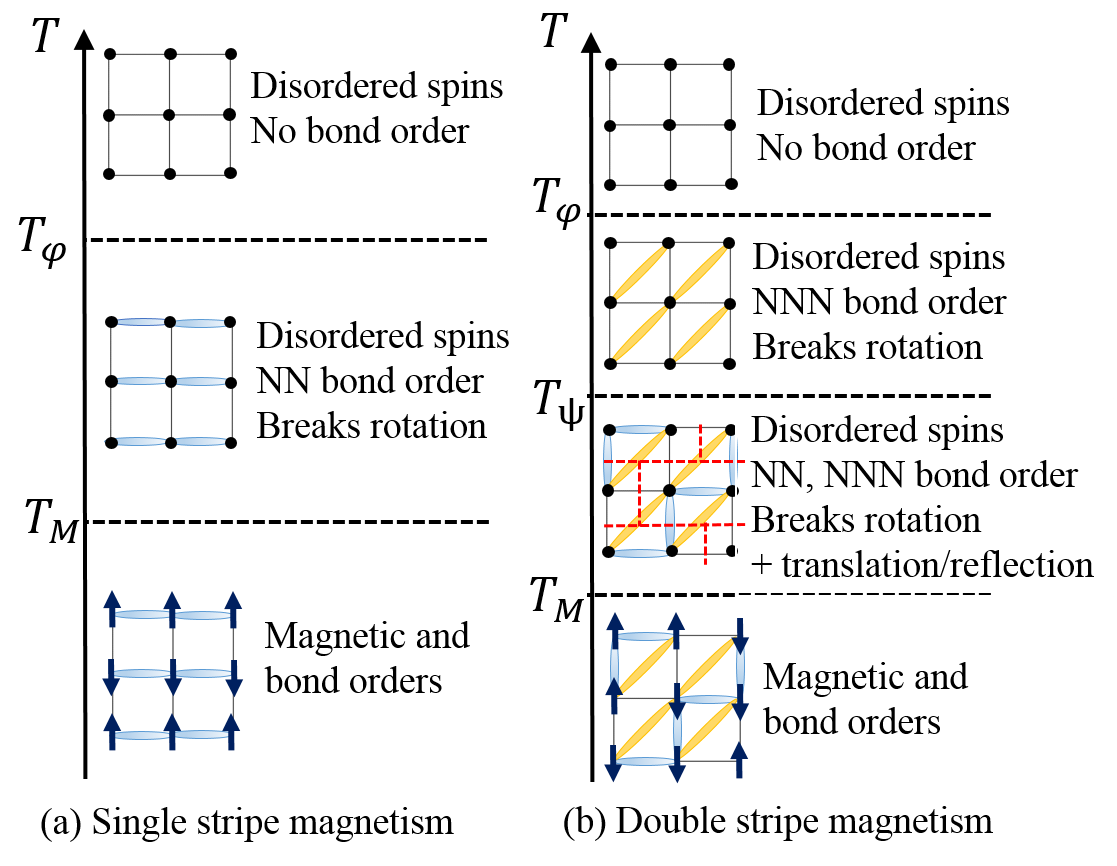
Figure 1: Multi-stage melting of the magnetic order in a square lattice as occurs in (a) single-stripe (SS) magnetism, and (b) double-stripe (DS) magnetism. The nearest (next-nearest) neighbor ferromagnetic bonds are indicated with blue (yellow) ovals. While in (a) there is one nematic bond-order degree of freedom associated with rotational symmetry-breaking, in (b) two bond-order degrees of freedom are associated with rotation, translation and reflection symmetry breaking. The new two site unit cell associated with the translation symmetry is indicated by the red dashed line.

II General properties of the double-stripe phase and its nematic phases

The phenomenon of partial melting of magnetically-ordered states, which is ultimately behind the onset of nematic phases, is caused by long-wavelength magnetic fluctuations (either thermal or quantum). Therefore, only approaches that go beyond mean-field can capture this effect. Here, as explained below in more detail, this will be achieved via a large-$N$ solution of the free energy functional for the DS state. Before we introduce it, we first discuss the different types of bond-order that appear in the DS ordered state, contrasting them with the standard SS ordered state.

II.1 Brief review of single-stripe magnetism and nematicity

Spin-driven nematicity in SS states is most straightforwardly discussed by means of a Heisenberg spin Hamiltonian. Following Ref. Chandra et al., 1990, we consider the following Hamiltonian for classical spins on the two-dimensional square lattice Chandra et al. (1990),

$$H=J_{1}\sum_{\langle ij\rangle}\mathbf{S}_{i}\cdot\mathbf{S}_{j}+J_{2}\sum_{\langle\langle ij\rangle\rangle}\mathbf{S}_{i}\cdot\mathbf{S}_{j}-K_{1}\sum_{\langle ij\rangle}\left(\mathbf{S}_{i}\cdot\mathbf{S}_{j}\right)^{2},$$ (1)

where $J_{1}$ and $J_{2}>0$ are nearest and next-nearest neighbor exchange couplings, and $K_{1}>0$ is the nearest-neighbor biquadratic coupling. In the context of the Fe-pnictides, which are metals with itinerant Fe electrons, such a model should be interpreted as an effective low-energy model to describe the interplay between SS magnetism and nematicity. Indeed, the inappropriateness of a purely localized approach is manifested by the fact that DFT calculations Yaresko et al. (2009); Glasbrenner et al. (2014) not only give soft moments, but also a large biquadratic exchange $K_{1}$ as compared to $J_{2},$ consistent with the experiment Wysocki et al. (2011). In contrast, the order-by-disorder mechanism of Ref. Chandra et al., 1990 gives a rather small $K_{1}/J_{2}\sim 10^{-3}$ Singh et al. (2003).

Single-stripe magnetism and the related nematicity occurs for $J_{2}>J_{1}/2$, and is most simply understood by taking $J_{2}\gg J_{1}$, where $J_{2}$ leads to two decoupled antiferromagnetic Néel sublattices. $J_{1}$ cannot couple these two sublattices, as the exchange fields between sublattices one and two cancel. However, the biquadratic term, $K_{1}$ requires that the spins be collinear, leading to two degenerate ground states where the spins are ferromagnetically correlated along either $\hat{x}$ or $\hat{y}$, and antiferromagnetically correlated along the perpendicular direction. These two degenerate ground states can be described by the wave-vectors $(0,\pi)$ and $(\pi,0)$, respectively, and break both the continuous spin-rotation symmetry, and the discrete $C_{4}$ lattice rotation symmetry (i.e. the symmetry of a square) down to $C_{2}$ (i.e. the symmetry of a rectangle), as shown in the bottom left of Fig. 1. These broken symmetries can be captured by three different order parameters: two of them are vector Néel order parameters, $\langle\mathbf{M}_{1}\rangle$ and $\langle\mathbf{M}_{2}\rangle$ defined on each sublattice, and a bond-order parameter describing the rotational symmetry breaking,

$$\varphi =\frac{1}{N_{s}}\sum_{i}\langle\mathbf{S}_{i}\cdot\mathbf{S}_{i+\hat{x}}-\mathbf{S}_{i}\cdot\mathbf{S}_{i+\hat{y}}\rangle$$

$$=\langle\mathbf{M}_{1}\cdot\mathbf{M}_{2}\rangle,$$ (2)

where $N_{s}$ is the number of sites. Effectively, the sign of $\varphi$ describes the orientation of the ferromagnetic bonds, either along $\hat{x}$ ($\varphi>0$) or along $\hat{y}$ ($\varphi<0$), while the magnitude of $\varphi$ describes the strength of both the ferro- and antiferromagnetic bonds.

The Mermin-Wagner theorem precludes any magnetic order at any finite temperature, in a strict two-dimensional lattice, as it breaks continuous spin-rotation symmetry. Therefore, the Néel order parameters, $\langle\mathbf{M}_{1}\rangle=\langle\mathbf{M}_{2}\rangle=0$. However, $\varphi$ is a scalar (Ising) order parameter and breaks only the discrete $C_{4}$ symmetry, and so it that can, and does, condense at a finite temperature. While $\varphi$ is called a nematic order parameter because it describes how the magnetic fluctuations break $C_{4}$ symmetry, it can more generally be thought of as a scalar bond order parameter that breaks a discrete lattice symmetry, which we shall generalize onto the case of DS magnetism. Here, although the spins themselves are slowly fluctuating, the correlation of the fluctuations between the two sublattices provides additional free energy gain and generates a long-range order without breaking any continuous symmetry. In momentum space, one can imagine that there is short range order at both $\mathbf{Q}=(0,\pi)$ and $(\pi,0)$ above $T_{\varphi}$, while below $T_{\varphi}$ the fluctuations increase at one $\mathbf{Q}$ vector and decrease at the other, thus breaking the rotational symmetry Fernandes et al. (2012). This has indeed been observed experimentally by neutron scattering in the iron pnictides Lu et al. (2014).

Realistic systems will have some finite inter-layer coupling $J_{\perp}$ that allows magnetism to develop at a temperature $T_{M}$ governed by $\ln\left(J_{\perp}/J_{2}\right)$, at which point long-range magnetic order will develop at the $\mathbf{Q}$ vector already chosen by $\varphi$. For sufficiently small $J_{\perp}$, these two temperature scales can remain separate Fang et al. (2008); Xu et al. (2008), although they will typically merge for sufficiently large $J_{\perp}$ Fernandes et al. (2012); Kamiya et al. (2011a), as the three-dimensionality reduces the role of magnetic fluctuations.

II.2 Double-stripe magnetism and nematicity: symmetry analysis

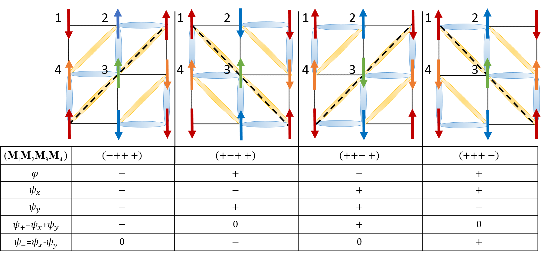
Figure 2: (Color online)The four degenerate ground states characterized by different configurations of $\mathbf{M}_{a}$’s and signs of corresponding order parameters $\varphi$, $\psi_{x,y}$ and $\psi_{+}$. Again the ferromagnetic bonds are indicated with blue/yellow ovals. The dashed black line shows the mirror plane symmetry broken by $\psi_{\pm}$.

Double-stripe magnetism consists of a plaquette of four spins – three up, one down, repeated with a staggered, $(\pi,\pi)$ pattern, as shown in Fig. 1b, bottom panel, leading to an 4-site magnetic unit cell (see Fig . 8(a)). This ordering results in double-width ferromagnetic stripes along the diagonal, alternating antiferromagnetically, hence the name double-stripe (DS). The DS pattern can be thought of as two copies of single-stripe orders in “even” and “odd” sublattices, rotated by $45^{\circ}$ and then coupled together by another biquadratic coupling. In this case, the effective low-energy Hamiltonian that displays this ground state in the classical regime is:

$$H=J_{1}\sum_{\langle ij\rangle}\mathbf{S}_{i}\cdot\mathbf{S}_{j}+J_{2}\sum_{\langle\langle ij\rangle\rangle}\mathbf{S}_{i}\cdot\mathbf{S}_{j}+J_{3}\sum_{\langle\langle\langle ij\rangle\rangle\rangle}\mathbf{S}_{i}\cdot\mathbf{S}_{j}\\ -K_{1}\sum_{\langle ij\rangle}\left(\mathbf{S}_{i}\cdot\mathbf{S}_{j}\right)^{2}-K_{2}\sum_{\langle\langle ij\rangle\rangle}\left(\mathbf{S}_{i}\cdot\mathbf{S}_{j}\right)^{2}\\ +R_{1}\sum_{\text{plaquette}}\left[(\mathbf{S}_{i}\cdot\mathbf{S}_{j})(\mathbf{S}_{k}\cdot\mathbf{S}_{l})+(\mathbf{S}_{i}\cdot\mathbf{S}_{l})(\mathbf{S}_{k}\cdot\mathbf{S}_{j})\right]\\ -R_{2}\sum_{\text{plaquette}}\left[(\mathbf{S}_{i}\cdot\mathbf{S}_{k})(\mathbf{S}_{j}\cdot\mathbf{S}_{l})\right]$$ (3)

where $\langle\rangle$, $\langle\langle\rangle\rangle$, and $\langle\langle\langle\rangle\rangle\rangle$ denote the first, the second and the third nearest neighbors, respectively. The $\sum_{\text{plaquette}}$ is defined such that $ijkl$ are the indices circulating a square plaquette. Note that the ring exchange terms are often included with an approximation $R\equiv R_{1}=R_{2}$ (which we also used in our DFT fits in Section III.2), but for itinerant systems the two coefficients can, in principle, be different.

One can understand this model by first considering the limit where $J_{3}>0$ is the dominant interaction. If $J_{3}$ plays the pivotal role in the spin dynamics, it is natural to partition the system into four antiferromagnetic Néel sublattices, so that $J_{3}$ is the nearest neighbor coupling for each of them, as shown in Fig. 2. Then the $J_{2}-J_{3}$ model describes two copies of SS magnetism. The biquadratic terms, $K_{1}>0$ and $K_{2}>0,$ force all four sublattices to be collinear. However, the DS and plaquette (Fig. 3) orders are exactly degenerate unless the ring exchange terms are included Glasbrenner et al. (2015). Ab-initio calculations (see Section III) indicate that the DS pattern is the ground state, and also that the 4th order terms are sufficiently strong to severely penalize noncollinear states. To simplify our analysis while still accounting for these details, we will drop both the ring exchange terms and only keep solutions corresponding with the symmetry of the DS ground state. We also drop $J_{1},$ which generates undesirable spiral solutions that we know are not present in our DFT calculations. Thus, we retain only the terms relevant to DS order, which are $J_{2,}$ $J_{3,}$ $K_{1}$, and $K_{2}$.

Besides the continuous spin-rotational symmetry, DS order also breaks a number of discrete symmetries. One can more clearly see those discrete symmetries by highlighting the location of the ferromagnetic bonds, as we have done in Fig. 2, for the four degenerate ground states. They are: the translational symmetry, since the unit cell is quadrupled in size; the $C_{4}$ rotational symmetry, which is broken along the diagonals of the squares ($B_{2g}$ symmetry) instead of along the sides of the square ($B_{1g}$ symmetry), as it was the case for the SS order; and the reflection symmetry ($\sigma_{d}$) across one of the diagonals ($x=\pm y$ lines). Unlike the “broken” translation symmetry of the single-stripe antiferromagnet, which can be restored by a time-reversal operation (or a 180^∘ rotation), here the layout of the NN ferromagnetic/antiferromagnetic bonds breaks translation symmetry and doubles the unit cell, which is doubled again when long-range magnetic order condenses, as shown in Fig. 1. In momentum space, this corresponds to 2$\mathbf{Q}$ ordering, with pairs of $\mathbf{Q}=(\pm\pi/2,\pm\pi/2)$ that are chosen to break the rotational symmetry appropriately. Note that in the case of the Ti-based oxypnictides discussed in the next section, some of those symmetries are already broken in the nonmagnetic phase due to crystallography.

To formally describe these discrete symmetries in terms of the spins, we consider the four Néel order parameters $\langle\mathbf{M}_{a}\rangle$ related to each of the four sublattices $a=1,2,3,4$ defined in Fig. 2. We first define the two next-nearest-neighbor bond orders, which couple to $K_{2}$:

$$\varphi_{\mathrm{odd}} =\langle\mathbf{M}_{1}\cdot\mathbf{M}_{3}\rangle$$ (4)

$$\varphi_{\mathrm{even}} =\langle\mathbf{M}_{2}\cdot\mathbf{M}_{4}\rangle$$ (5)

These order parameters characterize the emergence of diagonal bond order in the absence of long-range magnetic order, where $\varphi_{\mathrm{even/odd}}>0$ indicates which bonds within the four-spin plaquette are ferromagnetic. Fig. 3 shows that when $\varphi_{\mathrm{even/odd}}$ are opposite in sign, we can obtain the DS magnetic order, where each four-spin plaquette has an odd number of up and down spins. In contrast, when $\varphi_{\mathrm{even/odd}}$ have the same sign, we get the plaquette order discussed above. Note that, while we have drawn all spins as collinear, at this point the two sets of sublattices are decoupled and can rotate freely without affecting the bond order. By symmetry, $\varphi_{\mathrm{even/odd}}$ must condense at the same temperature, and indeed, it does not make sense to condense anything but a linear combination, $\varphi_{\mathrm{even}}\pm\varphi_{\mathrm{odd}}$, as each of $\varphi_{\mathrm{even/odd}}$ individually does not break a well-defined symmetry. Considering the bonds alone, $\varphi\equiv\varphi_{\mathrm{even}}-\varphi_{\mathrm{odd}}$ breaks the $C_{4}$ rotational symmetry, but not translation symmetry, while $\zeta\equiv\varphi_{\mathrm{even}}+\varphi_{\mathrm{odd}}$ doubles the unit cell, but maintains $C_{4}$ symmetry, as shown in Fig. 3. $\varphi$, of course, is consistent with DS order, while $\zeta$ is consistent with plaquette order, and these would be distinguished by the ring-exchange terms.

We have two reasons to believe that the DS order, and thus $\varphi$, is favored in the real materials. First, DFT calculations for both FeTe Glasbrenner et al. (2014) and the Ti-based oxypnictides considered in Sec. III show that the corresponding DS magnetic state is clearly lower in energy, which is consistent with the experimentally observed lattice distortions in the magnetic and/or putative nematic state. Second, $\varphi$ and $\zeta$ couple to different elastic modes and $\varphi$ may be additionally stabilized through magnetoelastic coupling Ducatman et al. (2014). In the following, we will neglect $\zeta$ and consider only the bond orders related to DS order.

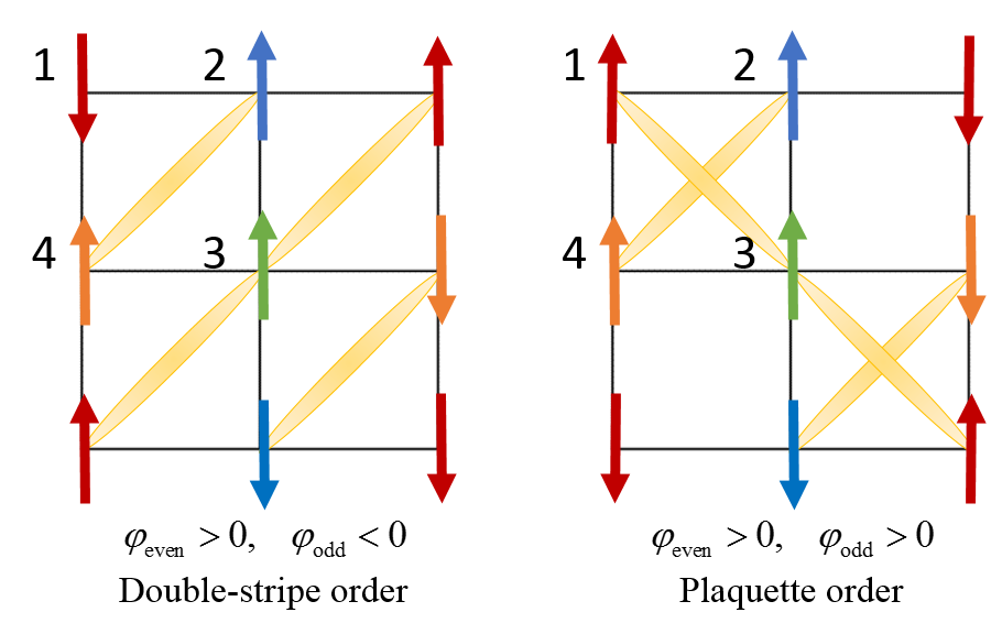
Figure 3: (Color online)Signs of $\varphi_{\mathrm{even/odd}}$ in a double-stripe order(left) and plaquette order(right).

Besides next-nearest neighbor bond-order, the DS order also has nearest-neighbor bond-orders, as shown in Fig. 2, which are driven by $K_{1}$. It is useful to define the generic bond-order parameter $\psi_{ab}=\langle\mathbf{M}_{a}\cdot\mathbf{M}_{b}\rangle$ on any pair of NN sublattices, i.e. $\psi_{12}$, $\psi_{14}$, $\psi_{23}$ and $\psi_{34}$. However, there are only two combinations of these that are compatible with a non-zero $\varphi$,

$$\psi_{\pm} =(\psi_{12}-\psi_{34})\pm(\psi_{14}-\psi_{23})$$

$$=\psi_{x}\pm\psi_{y}.$$ (6)

Each of these represents a pattern of alternating ferromagnetic and antiferromagnetic bonds along the $x$- and $y$-axes, resulting in a $(\pi,\pi)$ ordering pattern that doubles the unit cell. $\psi_{x/y}$ can be thought of as dimerization along the $x$-axis or $y$-axis respectively. Indeed, $\psi_{\pm}$ couple to a staggered strain associated with that dimerization of the lattice Paul et al. (2011). This symmetry breaking is also consistent with the intra-unit cell charge density wave observed in BaTi₂Sb₂O Frandsen et al. (2014); Song et al. (2016), which we will discuss further in Section III. In addition to translational symmetry, this bond order breaks the diagonal reflection symmetry, $\sigma_{d}$, across the line $x=\pm y$, for $\psi_{\pm}$ respectively. Finally, it breaks the same $C_{4}$ rotation symmetry as $\varphi$. In particular, because $\psi_{\pm}$ has ordering vector $\mathbf{Q}=\left(\pi,\pi\right)$, while $\varphi$ is a $\mathbf{Q}=0$ order, they can only couple via a linear-quadratic combination, i.e. $\varphi(\psi_{+}^{2}-\psi_{-}^{2})=\varphi\psi_{x}\psi_{y}$. Therefore, as soon as $\psi_{\pm}$ develops, $\varphi$ must also turn on, but the converse is not true.

Thus, besides the standard degeneracy related to spin-rotations, the DS ground state has an additional fourfold degeneracy related to the scalar order parameters $\varphi$ and $\psi_{\pm}$. These order parameters are not independent, as discussed above and shown in Fig. 2: $\varphi<0$ is only compatible with $\psi_{+}\neq 0$, whereas $\varphi>0$ is only compatible with $\psi_{-}\neq 0$. Therefore, the symmetry analysis of the DS state shows that when the magnetic ground state is the DS state, where $\varphi\neq 0$ and $\zeta=0$, we can have two partially-melted magnetic phases: one in which only $\varphi\neq 0$, which breaks rotational symmetry only, and another one in which both $\varphi\neq 0$ and $\psi_{\pm}\neq 0$, which breaks rotational symmetry, diagonal reflection symmetry, and translational symmetry. In the next section, we use a field-theory approach to discuss the order and character of these different transitions.

II.3 Double-stripe magnetism and nematicity: quantitative analysis

The bond order parameters $\varphi$ and $\psi_{\pm}$ discussed above can describe partially-melted DS phases, as long as they remain finite even in the absence of spin order, $\left\langle\mathbf{M}_{a}\right\rangle=0$. To characterize these phases, one needs to include magnetic fluctuations and therefore go beyond mean-field approaches. Within the specific spin Hamiltonian (3), this can be achieved numerically by Monte Carlo simulations Singh et al. (2003); Applegate et al. (2012) or analytically by $1/S$ expansions Chandra et al. (1990); Ducatman et al. (2012). Here, we employ a different approach, similarly to Ref. Fernandes et al., 2012, that relies on a low-energy Ginzburg-Landau free energy expansion of Eq. (3) in terms of the four real-space Néel order parameters $\mathbf{M}_{a}$ ($a=1,2,3,4$). As discussed above, this picture is valid in the limit where the third-neighbor magnetic coupling $J_{3}$ is by far the largest, and has been previously discussed for the double-stripe state Xu and Hu ; Ducatman et al. (2014). The most general form of the free energy expansion, with biquadratic exchanges taken into account, is:

$$F\left[\mathbf{M}_{i}\right]=\sum_{a,b=1}^{4}\int_{\mathbf{q}}\mathbf{M}_{a,\mathbf{q}}\chi_{ab}^{-1}\left(\mathbf{q}\right)\mathbf{M}_{b,-\mathbf{q}}\\ -\sum_{a,b,c,d=1}^{4}\int_{\mathbf{r}}\lambda_{ab,cd}\left(\mathbf{M}_{a}\cdot\mathbf{M}_{b}\right)\left(\mathbf{M}_{c}\cdot\mathbf{M}_{d}\right),$$ (7)

The Hamiltonian (3) generates numerous $\lambda$ terms, plus, if we allow for soft moments, as in a more itinerant model, terms with $a=b$ and/or $c=d$ are also allowed. However, most of these are irrelevant for the $\varphi$ and $\psi$ order parameters, so we will keep only the two combinations related to the DS order, and neglect the others. For the same reason, we will also retain one high-symmetry term accounting for softness of the magnetic moment. Then

$$F\left[\mathbf{M}_{i}\right]=\sum_{a,b=1}^{4}\int_{\mathbf{q}}\mathbf{M}_{a,\mathbf{q}}\chi_{ab}^{-1}\left(\mathbf{q}\right)\mathbf{M}_{b,-\mathbf{q}}+\frac{u}{2}\left(\sum_{a=1}^{4}\mathbf{M}_{a}^{2}\right)^{2}\\ -\frac{g_{1}}{2}\left(\mathbf{M}_{1}\cdot\mathbf{M}_{3}-\mathbf{M}_{2}\cdot\mathbf{M}_{4}\right)^{2}\\ -\frac{g_{3}}{2}\left[\left(\mathbf{M}_{1}\cdot\mathbf{M}_{2}-\mathbf{M}_{3}\cdot\mathbf{M}_{4}\right)^{2}\right.\\ \left.+\left(\mathbf{M}_{1}\cdot\mathbf{M}_{4}-\mathbf{M}_{2}\cdot\mathbf{M}_{3}\right)^{2}\right].$$ (8)

The physical meaning of each term can be understood from the Hamiltonian (3). The exchange couplings $J_{2}$ and $J_{3}$ describe the cost of spatial fluctuations of the order parameters, and appear in the non-uniform susceptibility $\chi_{ab}^{-1}\left(\mathbf{q}\right)$. As discussed in Appendix A, in our derivation we expand $\chi_{ab}^{-1}(\mathbf{q})$ around the ordering vector $\mathbf{Q=}\{\pi/2,\pi/2\},$ where $\chi_{ab}^{-1}(\mathbf{Q})=r_{0}\delta_{ab},$ and $r_{0}\propto T-T_{0}$, with $T_{0}$ denoting the mean-field magnetic transition temperature. The quadratic term in $\mathbf{(q-Q)}$ terms are then uniquely defined by $J_{2}$ and $J_{3}$. The $u$ term captures the cost of non-symmetry breaking longitudinal fluctuations. Together with the first term, it defines the amplitude of the local moments in the fully disordered case, as well as the softness of these moments. The four spin terms between next-nearest neighbors ($K_{2}$, $R_{2}$) lead to the $g_{1}$ term, which captures $\varphi$, while those between nearest-neighbors ($K_{1}$, $R_{1}$) lead to the $g_{3}$ terms, which in turn captures $\psi_{\pm}$ order.

In the mean-field approximation, the system develops DS order at $T_{0}$, simultaneous with $\varphi$ and $\psi_{\pm}$ bond orders in a second-order phase transition. To go beyond mean-field, we include the effect of the long wave-length fluctuations, working in two-dimensions, where magnetic order does not occur at any finite temperature due to the Mermin-Wagner theorem. Here, the fluctuations suppress the magnetic order to $T=0$. We then decouple the four quartic terms of Eq. (8) using Hubbard-Stratonovich transformations, which introduces four new scalar fields,

$$\varphi= g_{1}\left(\left\langle\mathbf{M}_{1}\cdot\mathbf{M}_{3}\right\rangle-\left\langle\mathbf{M}_{2}\cdot\mathbf{M}_{4}\right\rangle\right)$$ (9)

$$\psi_{x}= g_{3}\left(\left\langle\mathbf{M}_{1}\cdot\mathbf{M}_{2}\right\rangle-\left\langle\mathbf{M}_{3}\cdot\mathbf{M}_{4}\right\rangle\right)$$ (10)

$$\psi_{y}= g_{3}\left(\left\langle\mathbf{M}_{1}\cdot\mathbf{M}_{4}\right\rangle-\left\langle\mathbf{M}_{2}\cdot\mathbf{M}_{3}\right\rangle\right)$$ (11)

$$\eta= u\sum_{i=1}^{4}\langle\mathbf{M}_{i}^{2}\rangle,$$ (12)

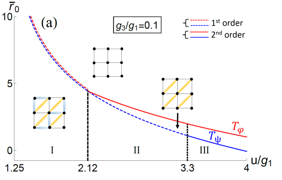
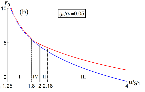
Figure 4: Two examples of how $\varphi$ and $\psi_{+}$ orders develop, with the proxy for the transition temperature, $\bar{r}_{0}$ plotted versus $u/g_{1}$ for two values of the relative strength of the biquadratic terms, $g_{3}/g_{1}$. The upper, red line indicates the development of rotational symmetry breaking ($\varphi$), while the lower, blue line indicates the dimerization ($\psi_{+}$), which breaks the diagonal mirror reflection symmetry. Solid lines indicate second order transitions, while dashed lines indicate first order transitions, with the double-dashed line indicating simultaneous first order transitions. The regions of different classes of behavior are indicated in Fig 5.

The scalar fields $\varphi$ and $\psi_{x/y}$ are equivalent to the bond order parameters introduced in the previous subsection, and therefore break the rotational symmetry ($\varphi$) and translational/reflectional symmetries ($\psi_{x/y}$, or $\psi_{\pm}$), and are not subject to the Mermin-Wagner theorem. On the other hand, $\eta$ is the mean-value of the Gaussian magnetic fluctuations, and simply renormalizes the magnetic transition temperature from its mean-field value $T_{0}$ to the value $T_{M}$ defined via $r=r_{0}+\eta\propto T-T_{M}$. Thus, $\eta$ is not an order parameter, as it is non-zero at any temperature.

To proceed, we consider the two-dimensional case, where magnetic order does not occur at any finite temperature, i.e. $\eta>-r_{0}$. In particular, we consider the large-$N$ solution of the free energy in Eq. (8), which is obtained by extending the number of components of the $\mathbf{M}_{a}$ fields from $3$ to $N$ and taking the limit $N\rightarrow\infty$. This yields a system of coupled self-consistent equations for $\varphi$, $\psi_{x}$, $\psi_{y}$, and $\eta$ (see detailed calculation in Appendix A). An important result of this calculation is that the first three scalar order parameters are not independent, but coupled in the free energy expansion according to the trilinear term, $\varphi\psi_{x}\psi_{y}.$ Furthermore, the combinations $\psi_{\pm}=\psi_{x}\pm\psi_{y}$ decouple from the self-consistent equations, indicating that $\psi_{x}$ and $\psi_{y}$ order simultaneously. Consequently, non-zero $\psi_{x/y}$ necessarily gives rise to a non-zero $\varphi$, as discussed in the previous subsection, whereas the converse is not true.

Therefore, we define two different bond-order transition temperatures: $T_{\varphi}$, which signals the onset of NNN bond-order $\varphi\neq 0$ (with $\psi_{\pm}=0$ and $M_{a}=0$), and $T_{\psi},$ which signals the onset of NN bond-order $\psi_{\pm}\neq 0$ (with $\varphi\neq 0$ and $M_{a}=0$). Note that whether $\psi_{+}$ or $\psi_{-}$ become non-zero depend on the sign of $\varphi$: while $\varphi>0$ gives $\psi_{-}\neq 0$, $\varphi<0$ gives $\psi_{+}\neq 0$ (see also Fig. 2).

In Fig. 4(a) and (b), we show two different classes of phase diagrams. The critical ${\bar{r}}_{0}\equiv r_{0}+8u\ln\Lambda$ (as defined in Appendix A), acts a proxy for temperature, and is plotted versus $u/g_{1}$ for two representative relative strengths of the biquadratic couplings, $g_{3}/g_{1}$. The NNN bond-order always onsets at the highest temperature, either alone ($T_{\varphi}>T_{\psi}$), in which case the transition can be either first or second order depending on $u/g_{1}$; or simultaneously with $\psi_{\pm}$ ($T_{\varphi}=T_{\psi}$), in which case the double transition must be first order. In the case $T_{\varphi}>T_{\psi}$, note that $T_{\psi}$ may be first or second order, depending on the parameter regime.

We can also understand these orders in momentum space, where the magnetic fluctuation spectrum at high temperatures is isotropic, with broad peaks at all four $\mathbf{Q}=\left(\pm\pi/2,\pm\pi/2\right)$ vectors. As the system cools down below $T_{\varphi}$, two combinations of the $\mathbf{Q}=\left(\pm\pi/2,\pm\pi/2\right)$ vectors develop stronger fluctuation amplitudes than the other two combinations, breaking the rotational symmetry. Upon further cooling to below $T_{\psi}$, the two sets of fluctuations become phase correlated.

As we have two control parameters, $u/g_{1}$ and $g_{3}/g_{1}$, we can explore a two-dimensional phase space, as indicated in Fig. 5. There are five different regimes of behavior. I: $\varphi$ and $\psi_{+}$ turn on simultaneously at a first order transition. II: $\varphi$ turns on continuously, with a second order transition, followed by a first order transition of $\psi_{+}$. III: two distinct second order phase transitions of $\varphi$ and $\psi_{+}$. IV: two distinct first order transitions of $\varphi$ and $\psi_{+}$. V: a first order transition to $\varphi$ followed by a second order transition to $\psi_{+}$. Note that these results are strongly dependent on the two-dimensionality: any finite inter-layer coupling will genreate a finite temperature magnetic phase transition. For relatively weak couplings, the phase diagrams can be quite complicatedZhang et al. , although as the couplings approach the three-dimensional limit, all three transitions will become first order and simulataneous, and there are no pre-emptive nematic transitions, as in the single-stripe case Fernandes et al. (2012, 2014); Chubukov et al. (2015); Xu et al. (2008); Fang et al. (2008); Abrahams and Si (2011); Mazin and Johannes (2009); Kamiya et al. (2011b); Capati et al. (2011); Brydon et al. (2011); Liang et al. (2013); Yamase and Zeyher (2015).

Figure 5: (Color online) Classes of phase transition behavior as the relative strength of the biquadratic terms, $g_{3}/g_{1}$ and $u/g_{1}$ are varied. I: Simultaneous first order transitions of $\varphi$ and $\psi_{+}$; II: Second order transition to $\varphi$ followed by a first order transition to $\psi_{+}$; III: Distinct second order phase transitions of $\varphi$ and $\psi_{+}$; IV: Distinct first order transitions of $\varphi$ and $\psi_{+}$; V: First order transition to $\varphi$ followed by a second order transition to $\psi_{+}$.

III Titanium-based oxypnictides

In the previous section we outlined the general theory of two-stage spin-driven nematicity, which made no assumptions about the chemical composition of the system. We now consider a real-world example using ab-initio DFT calculations that show that our model may be realized in the Ti-based oxypnictide BaTi₂Sb₂O. We begin by reviewing what is known experimentally about this family of materials followed by a brief discussion of previous DFT results. We detail our computational methods and present our calculations, which we discuss in the context of the model. The model and DFT results provide a consistent framework for interpreting what is known from experiment and indicates that magnetic fluctuations drive phenomena such as the nematic phase and the recently observed charge density wave.

III.1 Experimental status

The family of Ti-based oxypnictides contains two groups of compounds, BaTi₂Pn₂O (Pn = As, Sb, Bi) and Na₂Ti₂Pn₂O (Pn = As, Sb). These materials share common features, such as having layered tetragonal crystal structures similar to the Fe-based superconductors and with most compounds also exhibiting a density wave transition (the transition is suppressed in BaTi₂Bi₂O Yajima et al. (2012a, 2013)). The density wave transition occurs at $T_{DW}=50$ K for BaTi₂Sb₂O Yajima et al. (2012b); Doan et al. (2012), $T_{DW}=200$ K for BaTi₂As₂O Wang et al. (2010), and $T_{DW}=330$ K and $120$ K for the respective Na₂Ti₂Pn₂O (Pn = As, Sb) materials Adam and Schuster (1990); Ozawa et al. (2000, 2001). A subset of these compounds are superconductors, with BaTi₂Sb₂O being the prototypical example Yajima et al. (2012b); Doan et al. (2012) with a critical superconducting temperature of $T_{c}=1.2$ K Yajima et al. (2012b). Suppressing the density wave by substituting K for Ba increases $T_{c}$ up to $T_{c}=6.1$ K Pachmayr and Johrendt (2014), meaning that, as in the Fe-based superconductors, there is a correlation between superconductivity and the suppression of the density wave transition. However the critical superconducting temperatures are much smaller, so there is interest in understanding the differences between the Ti-based and Fe-based pnictides.

There is an active debate regarding the microscopic details and origin of the density wave (DW) transition in the Ti-based oxypnictides that hinges on two primary questions: 1) Is it a charge-density wave or a spin-density wave, and 2) what is the wave-vector of the DW? A set of NMR measurements, while not being able to resolve whether or not the DW has a charge or magnetic origin Kitagawa et al. (2013), placed symmetry constraints on the DW, finding that it broke the four-fold rotational symmetry at the Sb sites without enlarging the unit cell, making an incommensurate DW unlikely. Neutron powder diffraction measurements Frandsen et al. (2014) tightened these constraints by detecting a lattice distortion that accompanies the DW, changing the space group from $P4/mmm$ to $Pmmm$ due to a breaking of the four-fold rotational symmetry, but follow-up electron diffraction measurements did not detect a change in the number of Ti atoms per unit cell. The authors Ref. Frandsen et al., 2014 identified this as a nematic phase similar to what is observed in the Fe-based superconductors and proposed an “intra-unit-cell” charge-density wave to explain their results. This contrasts with Ref. Song et al., 2016, where the authors claim to have detected a CDW with wave-vector $\mathbf{Q}=(\pi,\pi)$ using angle-resolved photoemission spectroscopy and scanning tunneling microscopy measurements. This would mean that the DW breaks both rotational and translational symmetry and increases the unit cell size to four Ti sites, which is incompatible with the $Pmmm$ symmetry reported in Ref. Frandsen et al., 2014. In addition, while a long-range spin-density wave has yet to be detected in BaTi₂Sb₂O, none of these experiments have ruled out the potential existence of magnetic fluctuations around and below the DW transition temperature.

III.2 Density functional theory calculations

While experimental measurements of BaTi₂Sb₂O have yet to detect magnetism, DFT calculations Singh (2012); Suetin and Ivanovskii (2013); Wang et al. (2013) show a preference for magnetism in BaTi₂Sb₂O and predict the ground state to be the double stripe pattern. Including electronic correlations with the DFT+U correction further stabilizes the tendency towards magnetism Wang et al. (2013). In contrast, nonmagnetic calculations predict a phonon instability at $\mathbf{Q}=(\pi,\pi)$ in the high temperature structure Subedi (2013); Nakano et al. . Similar to experiment, the DFT calculations appear to point in multiple and exclusive directions, which complicates analysis of the DW transition and leaves open the possibility that the superconductivity in BaTi₂Sb₂O could be either conventional (electron-phonon coupling) or unconventional (spin-fluctuation mediated).

Many of these conflicts observed in both theory and experiment can be equitably resolved in our model, provided it is applicable to BaTi₂Sb₂O. To establish this, we calculate exchange parameters using DFT calculations, which confirms that BaTi₂Sb₂O is in the double-stripe regime described in Section II.3. We also revisit the nonmagnetic phonon instability and compare it with structural relaxations performed on the double stripe magnetic state, where we observe that the double-stripe magnetic pattern calculations yields a charge imbalance on two inequivalent Ti sites along with a orthorhombic distortion, which is consistent with our model and also the results of Ref. Frandsen et al., 2014. We conclude that this provides strong evidence that the DW transition corresponds to a spin-fluctuation-driven nematic intra-unit-cell CDW that breaks four-fold rotational symmetry.

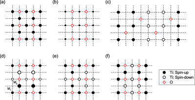
Figure 6: Schematic illustrating the different magnetic patterns considered in our collinear calculations. The inequivalent Ti sites are labeled as $M_{1}$ and $M_{2}$ in panel (d), and indicate NNN FM bonds bridging oxygen or vacancy sites, respectively. The relative sizes of the circles representing the Ti sites show the variation in local moment amplitudes (based on LSDA$+U$ calculations with $U=3.5\text{ eV}$) across the magnetic patterns. (a) Ferromagnetic (FM), (b) Checkerboard (CB), (c) Parallel stripes, (d) Double stripes (DS), (e) Oxygen-centered plaquettes (f) Vacancy-centered plaquettes.

III.2.1 Computational methods

Additional details of our DFT calculations can be found in Appendix B. In most calculations, we used the all-electron code elk elk , with testing selected calculations against the WIEN2k code Blaha et al. (2001). For the exchange-correlation potential we used both the local spin-density approximation (LSDA) Perdew and Wang (1992) and the generalized gradient approximation (GGA) Perdew et al. (1996) when computing collinear magnetic energies. To account for correlations on Ti, we used the DFT$+U$ method in the fully localized limit Liechtenstein et al. (1995), using two values of $U$, $2.5\text{ eV}$ and $3.5\text{ eV}$, and $J=0.5\text{ eV}$. Due to computational expense only the LSDA$+U$ functional with $U=3.5\text{ eV}$ was used in noncollinear calculations.

We used the experimental crystal structure in all of our calculations Doan et al. (2012). The space group symmetry is $P4/mmm$ and the lattice parameters were set to a = 4.1196 Å and c = 8.0951 Å. The Wyckoff positions for the atoms, given in fractional coordinates, are: Ba [1d] (0, 0, 0), Ti [2f] (0, 0.5, 0.5), Sb [2g] (0.5, 0.5, 0.2514), and O [1c] (0, 0, 0.5). The raw results of these calculations are presented in Appendix B.2.

The computed DFT energies were fit to the Hamiltonian in Eq. 3, which includes the lowest-order ring exchange terms. We included this term to capture the energy difference between the plaquette and double stripe configurations. Note that we assumed $R_{1}=R_{2}\equiv R$ for our fits.

The crystallography of the Ti-based oxypnictides complicates the comparison between these materials and the model described above both by breaking symmetries and modifying exchange interactions. With regards to the exchange interactions, the positions of the O atoms in the two-dimensional Ti₂O plane, see for example the schematics in Fig. 6, call for two types of NNN Ti-Ti bonds, those that are bridged by an O and those that are not. The consequences of this are two-fold: $J_{2}$ and $K_{2}$ are split into two unequal terms and in the DS magnetic pattern two Ti sites become inequivalent, see Fig. 6(d). Because of the moment softness the local moment amplitude of one site can be smaller by a factor of two when compared with the other (in the most extreme case the smaller moment collapses to zero, see Appendix B.2). In principle, this allows for two inequivalent DS patterns that differ depending on whether the FM bonds bridging O involve either large- or small-moment Ti sites. The moment softness also leads to different local moment amplitudes across magnetic patterns, which is illustrated in Fig. 6 by varying the relative size of the circles, which represent Ti sites, in the plots. While these complications are important for real Ti-based oxypnictides and is a likely source of the crystallographic complexity of the low-temperature phases, for simplicity we make the following assumptions when fitting to Eq. (3): we assume that the spins $S$ always have the same magnitude and normalize the values of $J$’s and $K$’s to $S=1$. For the purpose of mapping our calculations to the model described in Section II.3, we take the average the crystallographically inequivalent $J_{2}$’s, $K_{2}$’s and $R$’s (see Appendix B.1 and B.2).

For the nonmagnetic and long-range antiferromagnetic configurations we also performed structural relaxations using the projector augmented wave potentials in the pseudopotential code vasp Kresse and Hafner (1993); Kresse and Furthmüller (1996). One should keep in mind that, as we know from Fe-based superconductors, the role of the long magnetic order is to break the symmetry and create disbalance in orbital populations, which, in turn, couples to the lattice and generate a small lattice distortion. Many calculations for Fe pnictides and selenides show that the crystal structure in the symmetry-broken nematic states is very well described by the corresponding long-range ordered magnetic states, and we expect the same to be true here. In all our relaxations we fixed the volume to the experimental value and allowed the c/a ratio and ionic positions to relax. For the nonmagnetic instability, we considered the vanilla GGA Perdew et al. (1996) functional as well as the LSDA+U and GGA+U functionals with a rotationally invariant $U-J=3.0$ eV Dudarev et al. (1988), and for the double stripe relaxation we considered both LSDA+U and GGA+U with $U-J=3.0$ eV.

III.2.2 Results and discussion

We checked both the LSDA and GGA functionals with Hubbard $U$ values of 3.5 eV and 2.5 eV. GGA has more of a propensity towards magnetism, such that the GGA+$U=3.5$ eV calculations generated too large magnetic moments, thus we did not use this combination. We calculated the following magnetic patterns: ferromagnetic (FM), checkerboard (CB), double stripe (DS), oxygen- and vacancy-centered plaquettes, parallel stripes, and single stripes . Note that the DS states can be converged, when $U$ is included, to two different states differing by the local moment amplitude on the “weak” Ti site, which can either stay finite or collapse to zero Yu et al. (2014) (the relative amplitude is always smaller than the “strong” site). What is important is that the symmetry breaking remains the same in both cases, regardless of whether the “weak” site collapses. We also calculated the energy of ferromagnetic planes with antiferromagnetic stacking to get an estimate of the interplanar coupling. The energy calculations are summarized in Appendix B.2.

The fitted values of the exchange parameters that we obtained using LSDA$+U$ with $U=3.5\text{ eV}$ are $J_{1}=0.89\text{ meV}$, $J_{2}=-2.83\text{ meV}$, $J_{3}=2.79\text{ meV}$, $R=-0.26\text{ meV}$, $K_{1}=-0.37\text{ meV}$, and $K_{2}=2.06$. The full table of fitted parameters using different functionals and values of $U$ is available in Appendix B. While we note that there is noticeable variation of the absolute and even relative values of the exchange parameters across different functional and $U$ combinations, there are important qualitative observations we can make that hold in all cases: (1) the interaction is long-range, with $\lvert J_{2}\rvert>\lvert J_{1}\rvert$ and $J_{3}>(J_{1}-|J_{2}|)/2$ (the latter condition defines the double stripes as the mean-field ground state for sufficiently large $K$); this is an important prerequisite for the double-stage bond-orders described above. (2) $J_{2}$ is ferromagnetic in contrast to the Fe-based pnictides; however this sign difference is irrelevant to the model derived in the previous section. (3) There is a sizeable biquadratic coupling, $K_{2}>J_{3}/2>\lvert J_{2}\rvert/2>J_{1}/2$, $K_{1}+2R>J_{3}/2>\lvert J_{2}\rvert/2>J_{1}/2$, in which both $K_{1}$ and $K_{2}$ enforce collinearity. This ensures that spiral configurations play a minimal role and justifies setting $J_{1}$ to 0 in Section II.3. In addition, the distinction between $K_{1}$ and $R$ is subtle yet important, for if the latter is omitted from the fitting, $K_{1}$ turns positive, while including $R$ yields a $K_{1}$ that is slightly negative (in the Fe-based pnictides, including $R$ does not change the sign of $K_{1}$). In both cases, the strong NN quartic spin interactions enforce collinear spin patterns.

The calculated exchange parameters for LDA+U support the conclusion that BaTi₂Sb₂O is a real-world example of the model discussed in Section II.3, corresponding to a case where $J_{3}\gtrsim J_{1},J_{2}$ and $(K_{1}+2R)$, $K_{2}$ are positive and of the same order as the Heisenberg parameters. With this established, we now turn to discussing how the model and DFT results describe the nature of the density wave transition.

As previously discussed, due to the crystallography of BaTi₂Sb₂O the DFT calculation for the double stripe state has two inequivalent local Ti moments. The DFT calculations also show a charge imbalance between the inequivalent sites with there being $\sim 0.02$ more electrons at site $M_{2}$ (site with vacancy-bridging FM NNN interactions) compared to $M_{1}$ (site with oxygen-bridging FM NNN interactions), forming a pattern consistent with the intra-unit-cell charge-density wave reported in Ref. Frandsen et al., 2014 and in contrast to the $\mathbf{Q}=(\pi,\pi)$ charge-density wave argued for in Ref. Song et al., 2016, which would lead to four inequivalent Ti sites per unit cell. Furthermore, our spin-driven model is consistent with having an intra-unit-cell charge-density wave in the absence of long-range magnetic order. The argument is as follows: the presence of the oxygen sites breaks the translational symmetry of the hypothetical 1 Ti tetragonal cell, such that there are 2 Ti in the primitive unit cell even for $T>T_{\varphi}$. These Ti sites are differentiated by the direction of their oxygen coordination, along either $\hat{x}\pm\hat{y}$, and are related by rotational symmetry. However, when $T<T_{\varphi}$, the NNN bonds order, breaking this symmetry; for example see Fig. 7. The resulting FM bonds between Ti(1)-Ti(1) and Ti(2)-Ti(2) are inequivalent, with one bridging an oxygen and one bridging a vacancy. DFT calculations indicate that this inequivalency shows up as an intra-unit-cell charge-density wave. In addition, our model predicts that an initial unit cell with 2 inequivalent Ti sites will have nematic order and a charge-density wave condense at the same time, in complete agreement with experiment. Note that the mirror symmetry associated with $\psi_{\pm}$ remains unbroken until the NN bonds develop at $T_{\psi}$, even in the 2 Ti unit cell.

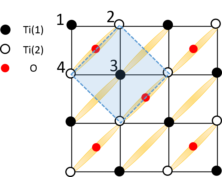
Figure 7: (Color online) In BaTi₂Sb₂O, there are two Ti sites [Ti(1), hollow circles and Ti(2), solid black circles] per unit cell, that are differentiated by the orientation of their oxygen coordination (red circles). The 2 Ti unit cell is shown by the blue, dashed lines. At high temperatures, these are equivalent and must carry the same charge, due to the rotation symmetry. However, below $T_{\varphi}$, the ferromagnetic bonds break rotation symmetry, and one Ti sublattice will have ferromagnetic bonds that cross oxygen sites, while the other will not, allowing a charge disproportionation to develop, such that $T_{\varphi}=T_{CDW}$.

Further support for the spin-driven case comes from our structural relaxation calculations, see Appendix B.3 for additional details. Similar to the Fe-based pnictides, structural relaxations of the DS pattern give rise to an orthorhombic distortion with $Pmmm$ symmetry (consistent with Ref. Frandsen et al. (2014)). The intra-unit-cell charge imbalance on the inequivalent Ti sites is also preserved after the optimization. In contrast, nonmagnetic calculations in the high temperature $P4/mmm$ structure yield a charge imbalance that resembles the double stripe pattern. As shown in previous studies Subedi (2013); Nakano et al. , this nonmagnetic charge density wave is unstable and promotes one of two lattice distortions, (i) A slight rotation of the Ti plaquettes centered around the oxygen sites as reported in Refs. Subedi, 2013; Nakano et al., , which breaks rotation and translation symmetries (but not the $\psi_{x/y}$ reflection symmetry) without an orthorhombic splitting of the in-plane a and b lattice parameters, or (ii) an orthorhombic distortion similar to what relaxing in the double stripe magnetic pattern yields, which does break rotational symmetry and splits the in-plane a and b lattice parameters. We stabilized both distortions in our structural relaxations, with the former distortion being lower in energy than the latter when using “vanilla” GGA or LSDA+U with $U-J=3.0\text{ eV}$. These relaxations also remove the charge imbalance on inequivalent Ti sites, implying that the distortions suppress the charge density wave.

It is important to emphasize that these nonmagnetic distortions are inconsistent with experiment: the Ti plaquette rotation does not break all the necessary symmetries, the energy of the orthorhombic distortion is higher than the plaquette rotation and within a tenth of a meV of the undistorted structure, and in both cases the distortion removes the charge imbalance on inequivalent Ti sites. Both nonmagnetic distortions are also significantly higher in energy than the magnetic double stripe configuration and its accompanying orthorhombic distortion for the LSDA+U functional. It is only within our spin-driven model that one obtains an orthorhombic lattice distortion with the correct symmetry, a charge imbalance on inequivalent Ti sites that persists after structural relaxation, and still not require that long-range magnetic order condense. The consistency of our model in explaining all observed phenomena also points to BaTi₂Sb₂O having a spin-fluctuation-mediated superconducting state.

IV Concluding remarks

We have presented an extension to the spin-driven nematic theory that describes fluctuations of double stripe magnetic order, which can break symmetries via a three-stage process. The first is the formation of second nearest-neighbor ferromagnetic bonds along one of the square diagonals, which breaks $C_{4}$ rotational symmetry, and the second is the formation of first nearest-neighbor ferromagnetic bonds in a staggered zig-zag pattern that breaks translational (doubling the unit cell) and reflection symmetries. Despite breaking different symmetries, these transitions are both bond-order transitions. In principle, in a quasi-three-dimensional system they should be followed by an antiferromagnetic transition, but, depending on the parameters and factors that go beyond the model, the magnetic transition may sink to an undetectable temperature. This happens, for instance, for SS nematicity in FeSe Glasbrenner et al. (2015). While this seems to also be the case for BaTi₂Sb₂O, where magnetic order has not been observed experimentally, in the DS compound FeTe the two bond-order transitions and the magnetic transition seem to be simultaneous and first-order. Going back to BaTi₂Sb₂O, where the magnetic transition is likely absent, the two bond order transitions can, in general, occur at either the same or different temperatures, depending on the relative amplitudes of the first- and second-nearest neighbor biquadratic exchange parameters and other factors, or the second transition may also sink to too-low temperatures. We speculate that the former may be the case in BaTi₂Sb₂O and the resulting merged phase transition is of very weak first order character. This would place BaTi₂Sb₂O in region I of the theoretical phase diagram of Fig. 5. Our DFT calculations confirmed that BaTi₂Sb₂O is within the regimes possible in this model and that all details of existing experiments can be accounted for in the spin-driven picture. The importance of spin fluctuations in explaining these phenomena suggests that the superconducting state may be unconventional and driven by spin fluctuations.

Direct confirmation of our theory should be possible with additional measurements. We predict that the BaTi₂Sb₂O exhibits correlated magnetic fluctuations without long-range order below the density wave transition temperature, similar to what is observed in paramagnetic nematic phases of specific iron pnictide superconductors, for example BaFe₂As₂. Techniques such as muon spin rotation, which have not found any evidence for magnetism in the titanium-based oxypnictides, are slow probes on the time-scale of magnetic fluctuations. Fast-probe techniques such as inelastic magnetic neutron scattering Diallo et al. (2010), photoemission spectroscopy Vilmercati et al. (2012), and x-ray emission spectroscopy Gretarsson et al. (2011) measurements are necessary to detect these fluctuations, as they have in the iron-based superconductors. A successful detection would provide direct evidence concerning the validity of our model. In addition, the model may also apply to other members of the titanium oxypnictide family, such as explaining the two phase transitions at $T=320\text{ K}$ (density wave) Ozawa et al. (2001) and $150\text{ K}$ (breaking of rotational symmetry) Chen et al. in Na₂Ti₂As₂O. Additional (magnetic) DFT calculations and experiments searching for magnetic fluctuations in Na₂Ti₂As₂O are therefore needed.

Appendix A Derivation of equations of state in effective field theory

In this appendix, we show briefly how to get the equations of state. After introducing the Hubbard-Stratonovich fields in eqns. (9)–(12), the free energy in Eq. (8) becomes:

$$F_{\mathrm{eff}}\left[\mathbf{M}_{i},\psi_{x/y},\varphi,\eta\right]=\\ \sum_{i,j=1}^{4}\int_{\mathbf{q}}\mathbf{M}_{i,\mathbf{q}}\chi_{ij}^{-1}\left(\mathbf{q}\right)\mathbf{M}_{j,-\mathbf{q}}-\varphi\left(\mathbf{M}_{1}\cdot\mathbf{M}_{3}-\mathbf{M}_{2}\cdot\mathbf{M}_{4}\right)\\ -\psi_{x}\left(\mathbf{M}_{1}\cdot\mathbf{M}_{2}-\mathbf{M}_{3}\cdot\mathbf{M}_{4}\right)-\psi_{y}\left(\mathbf{M}_{1}\cdot\mathbf{M}_{4}-\mathbf{M}_{2}\cdot\mathbf{M}_{3}\right)\\ +\eta\left(\sum_{i=1}^{4}\mathbf{M}_{i}^{2}\right)+\frac{\varphi^{2}}{2g_{1}}+\frac{\psi_{x}^{2}}{2g_{3}}+\frac{\psi_{y}^{2}}{2g_{3}}-\frac{\eta^{2}}{2u}.$$ (13)

Upon integrating out the $\mathbf{M}_{i}$, we obtain

$$F_{\mathrm{eff}}[\psi_{x,y},\varphi,\eta]=\\ \frac{T}{2}\int_{\mathbf{q}}\log\det\mathcal{G}_{\mathbf{q}}^{-1}+\frac{\varphi^{2}}{2g_{1}}+\frac{\psi_{x}^{2}+\psi_{y}^{2}}{2g_{3}}-\frac{\eta^{2}}{2u}$$ (14)

with $\mathcal{G}_{\mathbf{q}}^{-1}$ given by:

$$\begin{bmatrix}(r+J_{3}\delta q^{2})\mathbb{I}-\frac{\psi_{x}}{2}\sigma_{1}&-\frac{i\psi_{y}}{2}\sigma_{2}\!-\!(J_{2}\delta q_{x}\delta q_{y}\!+\!\frac{\varphi}{2})\sigma_{3}\!\!\\ \frac{i\psi_{y}}{2}\sigma_{2}\!-\!(J_{2}\delta q_{x}\delta q_{y}\!+\!\frac{\varphi}{2})\sigma_{3}\!\!\!&(r+J_{3}\delta q^{2})\mathbb{I}+\psi_{x}/2\sigma_{1}\end{bmatrix}$$ (15)

where $r\equiv r_{0}+\eta$.

The determinant of the inverse Green’s function is:

$$\det\mathcal{G}^{-1} =\frac{1}{16}\left(2\tilde{J}_{2}+2\tilde{J}_{3}+2r+\varphi-\psi_{x}-\psi_{y}\right)$$

$$\times\left(2\tilde{J}_{2}-2\tilde{J}_{3}-2r+\varphi+\psi_{x}-\psi_{y}\right)$$

$$\times\left(2\tilde{J}_{2}-2\tilde{J}_{3}-2r+\varphi-\psi_{x}+\psi_{y}\right)$$

$$\times\left(2\tilde{J}_{2}+2\tilde{J}_{3}+2r+\varphi+\psi_{x}+\psi_{y}\right)$$

$$=\left(\tilde{J}_{2}-\tilde{J}_{3}-\lambda\right)^{2}\left(\tilde{J}_{2}+\tilde{J}_{3}+\lambda\right)^{2}$$

$$+2\tilde{J}_{2}\left(\tilde{J}_{2}-\tilde{J}_{3}-\lambda\right)\left(\tilde{J}_{2}+\tilde{J}_{3}+\lambda\right)\varphi$$

$$+\frac{1}{2}\left(3\tilde{J}_{2}^{2}-(\tilde{J}_{3}+\lambda)^{2}\right)\varphi^{2}+\frac{\tilde{J}_{2}}{2}\varphi^{3}+\frac{\varphi^{4}}{16}$$

$$-\frac{1}{2}\left(\tilde{J}_{2}^{2}+(\tilde{J}_{3}+\lambda)^{2}\right)\left(\psi_{x}^{2}+\psi_{y}^{2}\right)$$

$$+2\tilde{J}_{2}(\tilde{J}_{3}+\lambda)\psi_{x}\psi_{y}+\frac{1}{16}\left(\psi_{x}^{2}-\psi_{y}^{2}\right)^{2}$$

$$+(\tilde{J}_{3}+\lambda)\varphi\psi_{x}\psi_{y}+\frac{\tilde{J}_{2}}{2}\varphi\left(\psi_{x}^{2}+\psi_{y}^{2}\right)$$

$$-\frac{1}{8}\varphi^{2}\left(\psi_{x}^{2}+\psi_{y}^{2}\right)$$ (16)

where we have introduced $\tilde{J}_{3}=J_{3}\delta q^{2}$ and $\tilde{J}_{2}=J_{2}\delta q_{x}\delta q_{y}$ for simplicity. In the Landau theory, we can expand the $\log\det\mathcal{G}^{-1}$ by assuming that everything involving $\varphi$, $\psi_{x}$ and $\psi_{y}$ is small in comparison to the first term. By doing so, we get a new Landau theory in terms of $\varphi$ and $\psi_{x/y}$. Once we do this expansion, we see that $\sum_{\mathbf{q}}\tilde{J}_{2}^{2n+1}$ type terms vanish. So the linear and cubic $\varphi$ terms vanish, as the $\varphi(\psi_{x}^{2}+\psi_{y}^{2})$ and $\psi_{x}\psi_{y}$ term. However, the $\varphi\psi_{x}\psi_{y}$ term is really there, as we expected. Since $\psi_{x}\psi_{y}$ acts like an external field for $\phi$, so either $\varphi$ turns on first, or $\psi_{x},\psi_{y}$ and $\varphi$ all turn on at the same time.

The next step is to minimize the effective action with respect to $\eta$, $\varphi$, $\psi_{x}$ and $\psi_{y}$ by taking the derivative of $S_{\mathrm{eff}}[\psi_{x},\psi_{y},\varphi,\eta]$ over $\psi_{x}$, $\psi_{y}$, $\varphi$ and $\eta$ respectively and force it to be zero. It is convenient to rewrite the action as:

$$S_{\mathrm{eff}}\left[\psi_{x},\psi_{y},\varphi,\eta\right]=\frac{\varphi^{2}}{2g_{1}}+\frac{\psi_{x}^{2}}{2g_{3}}+\frac{\psi_{y}^{2}}{2g_{3}}-\frac{\eta^{2}}{2u}$$ (17)

$$\quad+\frac{T}{2}\sum_{\mathbf{q}}\log\left(J_{3}q^{2}+J_{2}q_{x}q_{y}+r+\varphi-\psi_{x}-\psi_{y}\right)$$ (18)

$$\quad+\frac{T}{2}\sum_{\mathbf{q}}\log\left(J_{3}q^{2}-J_{2}q_{x}q_{y}+r-\varphi-\psi_{x}+\psi_{y}\right)$$ (19)

$$\quad+\frac{T}{2}\sum_{\mathbf{q}}\log\left(J_{3}q^{2}-J_{2}q_{x}q_{y}+r-\varphi+\psi_{x}-\psi_{y}\right)$$ (20)

$$\quad+\frac{T}{2}\sum_{\mathbf{q}}\log\left(J_{3}q^{2}+J_{2}q_{x}q_{y}+r+\varphi+\psi_{x}+\psi_{y}\right)\qquad$$ (21)

where we renormalize $\left(\varphi,\psi_{x},\psi_{y}\right)\rightarrow 2\left(\varphi,\psi_{x},\psi_{y}\right)$ and $g_{i}\rightarrow 4g_{i}$ for convenience. The saddle point equations $\frac{\partial S_{\mathrm{eff}}[x_{i}]}{\partial x_{i}}=0$($x_{i}=\eta,\varphi,\psi_{x}$ and $\psi_{y}$) become:

$$\eta =\frac{Tu}{2}\sum_{\mathbf{q}}\left[I_{1}\left(\mathbf{q}\right)+I_{2}\left(\mathbf{q}\right)+I_{3}\left(\mathbf{q}\right)+I_{4}\left(\mathbf{q}\right)\right]$$

$$\varphi =\frac{Tg_{1}}{2}\sum_{\mathbf{q}}\left[-I_{1}\left(\mathbf{q}\right)+I_{2}\left(\mathbf{q}\right)+I_{3}\left(\mathbf{q}\right)-I_{4}\left(\mathbf{q}\right)\right]$$

$$\psi_{x} =\frac{Tg_{3}}{2}\sum_{\mathbf{q}}\left[I_{1}\left(\mathbf{q}\right)+I_{2}\left(\mathbf{q}\right)-I_{3}\left(\mathbf{q}\right)-I_{4}\left(\mathbf{q}\right)\right]$$

$$\psi_{y} =\frac{Tg_{3}}{2}\sum_{\mathbf{q}}\left[I_{1}\left(\mathbf{q}\right)-I_{2}\left(\mathbf{q}\right)+I_{3}\left(\mathbf{q}\right)-I_{4}\left(\mathbf{q}\right)\right]$$ (22)

where $I_{l}(\boldsymbol{\mathbf{q}})(l=1,2,3,4)$ represents

$$I_{1}\left(\mathbf{q}\right) =\frac{1}{Jq^{2}+r+\varphi-\psi_{x}-\psi_{y}}$$

$$I_{2}\left(\mathbf{q}\right) =\frac{1}{Jq^{2}+r-\varphi-\psi_{x}+\psi_{y}}$$

$$I_{3}\left(\mathbf{q}\right) =\frac{1}{Jq^{2}+r-\varphi+\psi_{x}-\psi_{y}}$$

$$I_{4}\left(\mathbf{q}\right) =\frac{1}{Jq^{2}+r+\varphi+\psi_{x}+\psi_{y}}$$ (23)

In this, we have rotated our momentum axes to define the effective kinetic term $Jq^{2}=\sqrt{J_{3}^{2}-\frac{J_{2}^{2}}{4}}(\delta q_{x}^{2}+\delta q_{y}^{2})$ and renormalized $\left(\varphi,\psi_{x},\psi_{y}\right)\rightarrow 2\left(\varphi,\psi_{x},\psi_{y}\right)$ and $g_{i}\rightarrow 4g_{i}$ for convenience.

In the spirit of Landau theory, we next approximate $T$ by $T_{0}$ everywhere except in $r_{0}$, which we assume to be relatively small. We can then proceed to solve these equations in two dimensions by evaluating the momentum integrals $I_{l}(\mathbf{q})$ directly. These integrals diverge in the ultraviolet, so we must introduce a cutoff $\Lambda$. We can then absorb this into $\bar{r}_{0}=r_{0}+8u\ln\Lambda$. As the equations for $\psi_{x}$ and $\psi_{y}$ differ only by signs, we can decouple their equations by defining $\psi_{\pm}=\psi_{x}\pm\psi_{y}$, which have identical equations. The trilinear term $\varphi\psi_{x}\psi_{y}$ becomes $\varphi(\psi_{+}^{2}-\psi_{-}^{2})$. As only $\psi_{+}$ or $\psi_{-}$ will develop, depending on the sign of $\varphi$, we consider only $\psi_{+}$ ($\varphi<0$) and obtain the three saddle point equations,

$$\frac{\bar{r}_{0}-r}{u} =\ln(r+\varphi-\psi_{+})+\ln(r+\varphi+\psi_{+})+2\ln(r-\varphi)$$

$$\frac{\varphi}{g_{1}} =\ln(r+\varphi-\psi_{+})+\ln(r+\varphi+\psi_{+})-2\ln(r-\varphi)$$

$$\frac{\psi_{+}}{2g_{3}} =-\ln(r+\varphi-\psi_{+})+\ln(r+\varphi+\psi_{+})$$ (24)

where we have rescaled $\frac{T_{0}}{2J^{2}}(u,g_{1},g_{3})\rightarrow(u,g_{1},g_{3})$ and $\frac{1}{J}\left(\varphi,\psi_{+},r\right)\rightarrow\left(\varphi,\psi_{+},r\right)$ and absorbed a pre-factor $1/(4\pi)$ into the temperature $T_{0}$.

Appendix B DFT calculations

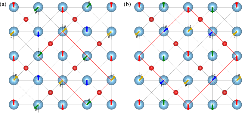
Figure 8: Schematics illustrating the four interpenetrating Néel sublattices (shown as different color vectors) that form the double stripe magnetic configuration and the two different $0\leq\theta\leq 180^{\circ}$ noncollinear rotations used in our DFT calculations to obtain the biquadratic terms $K_{1}$ and $K_{2}$. Red lines indicate the dimensions of the lateral supercell in each calculation. (a) Rotation analogous to a fluctuation of the $\psi_{\pm}$ order parameter (see Fig. 2). (b) Rotation analogous to a fluctuation of the $\varphi$ order parameter (see Fig. 2), which rotates between the $\mathbf{Q}=(\pi/2,\pi/2)$ and $(-\pi/2,\pi/2)$ configurations.

	LSDA+$U$						GGA+$U$
	U = 2.5 eV			U = 3.5 eV			U = 2.5 eV
Config	E - E(NM)	$M_{1}$	$M_{2}$	E - E(NM)	$M_{1}$	$M_{2}$	E - E(NM)	$M_{1}$	$M_{2}$
	(meV/Ti)	$(\mu_{B})$		(meV/Ti)	$(\mu_{B})$		(meV/Ti)	$(\mu_{B})$
FM	0.02993	0.2165	0.2165	-9.668	0.3761	0.3761	-21.761	0.4511	0.4511
CB	-0.2748	0.01661	0.01661	-13.241	0.1102	0.1102	-28.414	0.1648	0.1648
DS	-5.959	0.2631	0.3426	-20.950	0.3021	0.5537	-31.527	0.3452	0.5939
DS (O-FM only)	-3.674	0.3220	0.0000	-12.158	0.4783	0.0000	-16.642	0.5383	0.0000
DS (v-FM only)	-4.188	0.0000	0.4103	-18.291	0.0000	0.6167	-24.915	0.0000	0.6667
Parallel	-0.9796	0.1752	0.1752	-10.468	0.3891	0.3891	-22.384	0.4363	0.4363
Plaquette (O-centered)	-4.572	0.2503	0.2503	-16.022	0.3653	0.3653	-26.580	0.4015	0.4015
Plaquette (v-centered)	-4.269	0.3044	0.3044	-17.856	0.4535	0.4535	-29.084	0.4989	0.4989
AFM Layers	-0.6150	0.09566	0.09566	-9.154	0.3890	0.3890	-22.803	0.4866	0.4866

Table 1: A summary of the magnetic energies for the collinear magnetic patterns depicted in Fig. 6 using LSDA and GGA functionals and Hubbard $U$’s of 2.5 eV and 3.5 eV. The reported energies are referenced against the nonmagnetic (NM) state. For the DS patterns, the $M_{1}$ sites are those with NNN FM bonds bridging oxygen and $M_{2}$ are NNN FM bonds bridging vacancies. The “O-FM” and “v-FM” versions of DS are special cases when half the sites are nonmagnetic, with the magnetic sites either bridging across an oxygen site or a vacancy respectively. The plaquette patterns are labeled similarly, depending on whether they center around oxygen or vacancy sites.

In this Appendix we give additional details about how we performed the DFT calculations and also provide the raw results of our calculations along with additional discussion.

B.1 Computational methods: additional details

A method similar to that used in Ref. Glasbrenner et al., 2014 was employed for the noncollinear calculations that were used to extract the biquadratic interaction term. The configurations depicted in Figs. 8(a) and 8(b) indicate how we varied $\theta$ to calculate $E(\theta)$ for the two different setups. These involve rotations of the four Néel sublattices discussed in Section II.2, and in our calculations two of the sublattices are fixed and the other two are rotated to interpolate between degenerate double stripe configurations. Applying Eq. (3) to these configurations results in the following two expressions that we use for fitting:

$$E_{1}(\theta)-E_{1}(0) =2\left(K_{1}+2R\right)\sin^{2}\theta$$ (25)

$$E_{2}(\theta)-E_{2}(0) =\left(K_{1}+2K_{2}\right)\sin^{2}\theta.$$ (26)

$E_{1}(\theta)$ corresponds to Fig. 8(a) and $E_{2}(\theta)$ to Fig. 8(b). Note that the ring exchange enters as a term in Eq. (25)(a) , which we take from our collinear fits.

We used the following parameters in the calculations obtained using elk. For the k-mesh, we used a $14\times 14\times 8$ k-mesh for the ferromagnetic and checkerboard unit cells, a $12\times 8\times 8$ k-mesh for the double stripe cell (also used for noncollinear rotation in Fig. 8(a)), a $12\times 8\times 6$ k-mesh for the parallel stripes unit cell, a $14\times 14\times 4$ k-mesh for the antiferromagnetic layers unit cell, and a $8\times 8\times 8$ k-mesh for the plaquette unit cell (also used for noncollinear rotation in Fig. 8(b)). The number of empty states was set to 6 states/atom/spin. In addition, because of how elk evaluates the exchange-correlation potential, convergence of the $\theta=0$ and $\theta=180^{\circ}$ configurations in Fig. 8(b) (which are supposed to be degenerate) required setting the angular momentum cutoff for the APW functions (parameter lmaxapw) and the muffin-tin density and potential (parameter lmaxvr) to 10, and also reducing the fracinr parameter to 0.001 .

For our fittings to Eq. (3), as mentioned in the main text, the oxygen sites in BaTi₂As₂O lead to an anisotropy in the Ti-Ti NNN couplings, which in principle splits the second-neighbor Heisenberg exchange parameter ($J_{2}\to J_{2O},J_{2v}$), biquadratic exchange parameter (($K_{2}\to K_{2O},K_{2v}$)), and ring exchange parameter (($R\to R_{O},R_{v}$)). For consistency, we define a set of averaged exchange parameters to use when fitting: $2J_{2}=J_{2v}+J_{2O}$ for NNN Heisenberg exchange, $2K_{2}=K_{2O}+K_{2v}$ for NNN biquadratic exchange, and $2R=R_{O}+R_{v}$ for NNN ring exchange.

For our vasp structural relaxations, we used a plane wave energy cutoff of 600 eV. We also used the same k-meshes for the different supercell geometries as was used in the elk calculations.

B.2 Total energy calculations and fitted exchange parameters

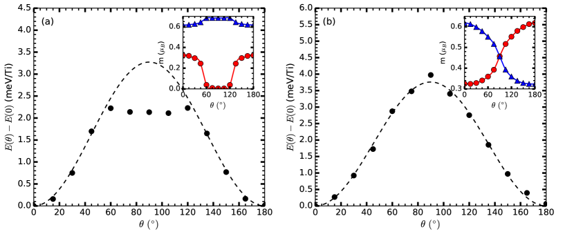
Figure 9: Noncollinear energies as a function of the rotation angle $\theta$. The dashed lines are the fits to the model. The insets in each panel show the inequivalent Ti local moments as a function of $\theta$. The red circles refer to NNN FM O-bridging Ti sites and the blue triangles to NNN FM vacancy-bridging Ti sites when $\theta=0$. (a) Noncollinear energies for the rotations analogous to fluctuations of the $\psi_{\pm}$ order parameter (see Fig. 8(a)). (b) Noncollinear energies for the rotations analogous to fluctuations of the $\varphi$ order parameter (see Fig. 8(b))

Table 1 contains the full summary of our total energy calculations and the Ti local moment amplitudes of the different magnetic patterns. We find that our results are consistent with the trends reported in Ref. Wang et al., 2013, where increasing $U$ lowers the energy of each configuration and increases the amplitude of the local moments. The local moments themselves are soft and can vary by more than a factor of 2 between magnetic patterns. Our calculations also capture the energy difference that arises due to the anisotropy in the $J_{2}$ parameter, which depends on whether the NNN ferromagnetic bonds bridge either an oxygen site or a vacancy. Overall NNN ferromagnetic bonds are energetically preferred.

The results of our noncollinear energy calculations are shown in Fig. 9, which we fit to Eqs. (25)–(26) to obtain the biquadratic parameters. In Fig. 9(a) the $M_{2}$ Ti moments collapse when $60^{\circ}\leq\theta\leq 120^{\circ}$; for simplicity we fit to Eq. (25) using only the energy calculations obtained for $\theta$ outside this range. As a side note, the rotations in Fig. 8 are analogous to the fluctuations discussed in Sections II.2 and II.3, with Fig. 8(a) being similar to fluctuations between the $(++-+)$ and $(-+++)$ states in Fig. 2 that are frozen out when $T<T_{\psi}$, and Fig. 8(b) being similar to fluctuations between the $(++-+)$ and $(+++-)$ states in Fig. 2 that are frozen out when $T<T_{\varphi}$.

Functional	$U$	$J_{1}$	$J_{2}$	$J_{3}$	$J_{\perp}$	$R$	$K_{1}$	$K_{2}$
	(eV)	(meV)
LDA+U	2.5	0.076	-1.04	1.59	0.32	0.38
LDA+U	3.5	0.89	-2.83	2.79	-0.26	1.00	-0.37	2.06
GGA+U	2.5	1.66	-2.41	1.89	0.52	0.92

Table 2: The calculated exchange parameters for BaTi₂Sb₂O.

The fitted exchange parameters are summarized in Table 2. For completeness, we included the interplanar coupling $J_{\perp}$ that was neglected in the model treatment. The sign of the Heisenberg and ring exchange parameters are consistent across functionals and values of $U$ with the exception of $J_{\perp}$, which is slightly ferromagnetic in LSDA$+U=3.5\text{ eV}$, but antiferromagnetic otherwise.

B.3 Structural relaxation data

Functional	$U-J$	Distortion	Energy	$Q(\text{Ti}_{1})$	$Q(\text{Ti}_{2})$	$\theta_{\text{Ti}}$	$\eta$
	(eV)		(eV/Ti)	(elec.)		(deg)	%
GGA	0.0	None	-19.59	10.2	10.2	0.0	0.0
GGA	0.0	Rotation	-19.59	10.2	10.2	3.5	0.028
GGA	0.0	Orthorhombic	-19.59	10.2	10.2	0.0	0.40
LSDA+U	3.0	None	-19.48	10.1	10.2	0.0	0.0
LSDA+U	3.0	Rotation	-19.48	10.2	10.2	2.19	0.08
LSDA+U	3.0	Orthorhombic	-19.48	10.1	10.2	0.0	0.51
LSDA+U	3.0	Double stripe	-19.49	10.2	10.1	0.0	1.4

Table 3: A summary of the results of structural relaxations of BaTi₂Sb₂O for different exchange-correlation functionals and kinds of distortions. The DFT+U calculations used the rotationally invariant approach with a single parameter $U-J$ Dudarev et al. (1988). The $Q(\text{Ti}_{1})$ and $Q(\text{Ti}_{2})$ columns report the calculated charge on the inequivalent Ti sites, the $\theta_{\text{Ti}}$ column reports how many degrees the oxygen-centered Ti plaquettes are rotated in each distortion (if at all), and the final column calculates $\eta=2\cdot\frac{a-b}{a+b}\cdot 100\%$, which quantifies the degree of the orthorhombic distortion.

The structural relaxations we computed using vasp are summarized in Table 3. For all functionals we first performed a baseline relaxation calculation where we enforced the high temperature structure with $P4/mmm$ symmetry. We then considered up to three kinds of distortions. The nonmagnetic distortions are the “rotation” distortion, which refers to rotations of Ti plaquettes about the oxygen sites by an angle $\theta_{\text{Ti}}$, and the “orthorhombic” distortion, which is a spitting of the $a$ and $b$ lattice parameters quantified with the parameter $\zeta=2\cdot\frac{a-b}{a+b}\cdot 100\%$. The “double stripe” distortion, on the other hand, is obtained by performing a structural relaxation for the magnetic double stripe pattern. We then compared the energies, the calculated charges on the two inequivalent Ti sites, and the distortion parameters $\theta_{\text{Ti}}$ and $\zeta$.

We found that for the vanilla DFT calculations with the GGA functional, the plaquette rotation distortion is lowest in energy, with E(rotation) - E(none) = -5.8 meV/Ti compared with E(orthorhombic) - E(none) = 0.03/Ti meV. The undistorted structures feature a charge imbalance on the inequivalent Ti sites, while the distorted sites do not. The rotated plaquettes structure also has a minor orthorhombic distortion of 0.03%, which is negligible.

For the LSDA+U (U - J = 3.0 eV) calculations, the double stripe distortion is clearly the lowest in energy, with E(ds) - E(none) = -18.4 meV/Ti compared with E(rotation) - E(none) = -0.88 meV/Ti and E(orthorhombic) - E(none) = -0.079 meV/Ti. The nonmagnetic distortions do not provide much of an energy gain, particularly when compared with the relaxed magnetic state. As in the case of vanilla GGA, the nonmagnetic distortions remove the charge imbalance between $M_{1}$ and $M_{2}$ found in the high temperature structure. In contrast, the charge imbalance still persists after relaxing the double stripe pattern.

In terms of symmetry breaking, only the relaxed magnetic calculations break rotational, reflection, and translational symmetry, induce a orthorhombic lattice distortion, and preserve a charge imbalance between the inequivalent Ti sites. The nonmagnetic distortions may or may not break the right symmetries compared with experiment, and after relaxation the charge imbalance disappears.

B.4 BaTi₂As₂O

Config	E - E(NM)	$M_{1}$	$M_{2}$
	(meV/Ti)	$(\mu_{B})$
FM	-0.8245	0.3116	0.3116
DS (O-FM only)	-4.562	0.3226	0.0000
DS (v-FM only)	-9.787	0.0000	0.4673
Parallel	-3.354	0.1987	0.1987
Plaquette (O-centered)	-4.843	0.2359	0.2359
Plaquette (v-centered)	-9.246	0.3260	0.3260
AFM Layers	-3.257	0.3242	0.3242

Table 4: The magnetic energies for the collinear magnetic patterns that are stable in BaTi₂As₂O for LSDA+U with $U=3.5\text{ eV}$ and $J=0.5\text{ eV}$. Energies are referenced against the nonmagnetic (NM) state. The inequivalent magnetic moments $M_{1}$ and $M_{2}$ in the double stripe and site-selective patterns are the same as those labeled in Fig. 6

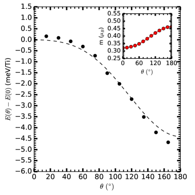
Figure 10: Noncollinear energies for rotations connecting the two double stripe patterns where one of the local Ti moments has collapsed. $\theta=0$ corresponds to moments with oxygen-bridging FM NNN interactions and $\theta=180^{\circ}$ to moments with vacancy-bridging FM NNN interactions. The dashed line is the fit to the model. The inset shows the Ti local moment as a function of $\theta$.

We performed a set of DFT calculations for BaTi₂As₂O in order to compare with the main BaTi₂Sb₂O results. These calculations used the LSDA+U functional with $U=3.5\text{ eV}$ and $J=0.5\text{ eV}$. We used the experimental crystal structure for these calculations Wang et al. (2010), which has space group symmetry $P4/mmm$, lattice parameters a = 4.04561 Åand c = 7.27228 Å, and the following Wyckoff positions in fractional coordinates: Ba [1d] (0.5, 0.5, 0.5), Ti [2f] (0.5, 0, 0), As [2g] (0, 0, 0.7560), and O [1c] (0.5, 0.5, 0). We used the same k-meshes and parameters as was used for BaTi₂Sb₂O.

The results of the collinear calculations are summarized in Table 4. BaTi₂As₂O is less supportive of magnetism compared to BaTi₂Sb₂O, as the full double stripe and checkerboard patterns cannot be stabilized and the stable patterns yield less of an energy gain compared to their BaTi₂Sb₂O counterparts. Because of this, there are not enough stable collinear magnetic patterns that we can use to fit to Eq. (3). Trying to include the patterns with nonmagnetic sites further complicates the model, as we would need to add Stoner-like on-site terms to capture variations in the local moments.

Even though we cannot resolve all the exchange parameters through a fit, we can at least estimate the NNN biquadratic parameter. We do this by performing noncollinear calculations with rotations that interpolate between the two kinds of double stripe patterns where half the sites are nonmagnetic. The results of these calculations are presented in Fig. 10. Applying Eq. (3), we obtain the following expression,

$$E(\theta)-E(0) =2K_{2}\sin^{2}\theta+2\left(J_{2v}-J_{2O}\right)\sin^{2}\left(\frac{\theta}{2}\right)$$ (27)

In Eq. (27) the anisotropic splitting of $J_{2}$ enters as a difference instead of a sum, so we can’t use the average value $J_{2}$ here. However, we also note that the energy difference between the two plaquette configurations is $E(\text{Plaq}_{v})-E(\text{Plaq}_{O})=2\left(J_{2v}-J_{2O}\right)$, which can be substituted in Eq. (27) to allow us to resolve $K_{2}$. We obtain $K_{2}=0.418\text{ meV}$ from this fit, but without $J_{2v}$, $J_{2O}$ and $J_{3}$ available for comparison, it is unclear what regime of the model in Section II.3 BaTi₂As₂O is in.

References

- Kivelson et al. (1998) S. A. Kivelson, E. Fradkin, and V. J. Emery, Nature 393, 550 (1998).
- Chandra et al. (1990) P. Chandra, P. Coleman, and A. I. Larkin, Phys. Rev. Lett. 64, 88 (1990).
- Fang et al. (2008) C. Fang, H. Yao, W.-F. Tsai, J. Hu, and S. A. Kivelson, Phys. Rev. B 77, 224509 (2008).
- Xu et al. (2008) C. Xu, M. Müller, and S. Sachdev, Phys. Rev. B 78, 020501 (2008).
- Mazin and Johannes (2009) I. I. Mazin and M. D. Johannes, Nat. Phys. 5, 141 (2009).
- Fernandes et al. (2012) R. M. Fernandes, A. V. Chubukov, J. Knolle, I. Eremin, and J. Schmalian, Phys. Rev. B 85, 024534 (2012).
- Fernandes et al. (2014) R. M. Fernandes, A. V. Chubukov, and J. Schmalian, Nat. Phys. 10, 97 (2014).
- Christensen et al. (2016) M. H. Christensen, J. Kang, B. M. Andersen, and R. M. Fernandes, Phys. Rev. B 93, 085136 (2016).
- Wang and Chubukov (2014) Y. Wang and A. Chubukov, Phys. Rev. B 90, 035149 (2014).
- Nie et al. (2014) L. Nie, G. Tarjus, and S. A. Kivelson, PNAS 111, 7980 (2014).
- Roy et al. (2015) B. Roy, J. Hofmann, V. Stanev, J. D. Sau, and V. Galitski, Phys. Rev. B 92, 245431 (2015).
- Yoshizawa et al. (2012) M. Yoshizawa, D. Kimura, T. Chiba, S. Simayi, Y. Nakanishi, K. Kihou, C.-H. Lee, A. Iyo, H. Eisaki, M. Nakajima, and S. ichi Uchida, J. Phys. Soc. Jpn. 81, 024604 (2012).
- Gallais et al. (2013) Y. Gallais, R. M. Fernandes, I. Paul, L. Chauvière, Y.-X. Yang, M.-A. Méasson, M. Cazayous, A. Sacuto, D. Colson, and A. Forget, Phys. Rev. Lett. 111, 267001 (2013).
- (14) H.-H. Kuo, J.-H. Chu, J. C. Palmstrom, S. A. Kivelson, and I. R. Fisher, “Ubiquitous signatures of nematic quantum criticality in optimally doped Fe-based superconductors,” arXiv:1503.00402 .
- Lederer et al. (2015) S. Lederer, Y. Schattner, E. Berg, and S. A. Kivelson, Phys. Rev. Lett. 114, 097001 (2015).
- (16) C. Xu and J. Hu, “Field theory for magnetic and lattice structure properties of Fe1+yTe1-xSex,” arXiv:0903.4477 .
- Li et al. (2009) S. Li, C. de la Cruz, Q. Huang, Y. Chen, J. W. Lynn, J. Hu, Y.-L. Huang, F.-C. Hsu, K.-W. Yeh, M.-K. Wu, and P. Dai, Phys. Rev. B 79, 054503 (2009).
- Bao et al. (2009) W. Bao, Y. Qiu, Q. Huang, M. A. Green, P. Zajdel, M. R. Fitzsimmons, M. Zhernenkov, S. Chang, M. Fang, B. Qian, E. K. Vehstedt, J. Yang, H. M. Pham, L. Spinu, and Z. Q. Mao, Phys. Rev. Lett. 102, 247001 (2009).
- Frandsen et al. (2014) B. A. Frandsen, E. S. Bozin, H. Hu, Y. Zhu, Y. Nozaki, H. Kageyama, Y. J. Uemura, W.-G. Yin, and S. J. L. Billinge, Nat. Commun. 5, 5761 (2014).
- Yaresko et al. (2009) A. N. Yaresko, G.-Q. Liu, V. N. Antonov, and O. K. Andersen, Phys. Rev. B 79, 144421 (2009).
- Glasbrenner et al. (2014) J. K. Glasbrenner, J. P. Velev, and I. I. Mazin, Phys. Rev. B 89, 064509 (2014).
- Wysocki et al. (2011) A. L. Wysocki, K. D. Belashchenko, and V. P. Antropov, Nat. Phys. 7, 485 (2011).
- Singh et al. (2003) R. R. P. Singh, W. Zheng, J. Oitmaa, O. P. Sushkov, and C. J. Hamer, Phys. Rev. Lett. 91, 017201 (2003).
- Lu et al. (2014) X. Lu, J. T. Park, R. Zhang, H. Luo, A. H. Nevidomskyy, Q. Si, and P. Dai, Science 345, 657 (2014).
- Kamiya et al. (2011a) Y. Kamiya, N. Kawashima, and C. D. Batista, Phys. Rev. B 84, 214429 (2011a).
- Glasbrenner et al. (2015) J. K. Glasbrenner, I. I. Mazin, H. O. Jeschke, P. J. Hirschfeld, R. M. Fernandes, and R. Valentí, Nat. Phys. 11, 953 (2015).
- Ducatman et al. (2014) S. Ducatman, R. M. Fernandes, and N. B. Perkins, Phys. Rev. B 90, 165123 (2014).
- Paul et al. (2011) I. Paul, A. Cano, and K. Sengupta, Phys. Rev. B 83, 115109 (2011).
- Song et al. (2016) Q. Song, Y. J. Yan, Z. R. Ye, M. Q. Ren, D. F. Xu, S. Y. Tan, X. H. Niu, B. P. Xie, T. Zhang, R. Peng, H. C. Xu, J. Jiang, and D. L. Feng, Phys. Rev. B 93, 024508 (2016).
- Applegate et al. (2012) R. Applegate, R. R. P. Singh, C.-C. Chen, and T. P. Devereaux, Phys. Rev. B 85, 054411 (2012).
- Ducatman et al. (2012) S. Ducatman, N. B. Perkins, and A. Chubukov, Phys. Rev. Lett. 109, 157206 (2012).
- (32) G. Zhang, R. M. Fernandes, and R. Flint, In preparation.
- Chubukov et al. (2015) A. V. Chubukov, R. M. Fernandes, and J. Schmalian, Phys. Rev. B 91, 201105 (2015).
- Abrahams and Si (2011) E. Abrahams and Q. Si, Journal of Physics: Condensed Matter 23, 223201 (2011).
- Kamiya et al. (2011b) Y. Kamiya, N. Kawashima, and C. D. Batista, Phys. Rev. B 84, 214429 (2011b).
- Capati et al. (2011) M. Capati, M. Grilli, and J. Lorenzana, Phys. Rev. B 84, 214520 (2011).
- Brydon et al. (2011) P. M. R. Brydon, J. Schmiedt, and C. Timm, Phys. Rev. B 84, 214510 (2011).
- Liang et al. (2013) S. Liang, A. Moreo, and E. Dagotto, Phys. Rev. Lett. 111, 047004 (2013).
- Yamase and Zeyher (2015) H. Yamase and R. Zeyher, New J. Phys. 17, 073030 (2015).
- Yajima et al. (2012a) T. Yajima, K. Nakano, F. Takeiri, J. Hester, T. Yamamoto, Y. Kobayashi, N. Tsuji, J. Kim, A. Fujiwara, and H. Kageyama, J. Phys. Soc. Jpn. 82, 013703 (2012a).
- Yajima et al. (2013) T. Yajima, K. Nakano, F. Takeiri, Y. Nozaki, Y. Kobayashi, and H. Kageyama, J. Phys. Soc. Jpn. 82, 033705 (2013).
- Yajima et al. (2012b) T. Yajima, K. Nakano, F. Takeiri, T. Ono, Y. Hosokoshi, Y. Matsushita, J. Hester, Y. Kobayashi, and H. Kageyama, J. Phys. Soc. Jpn. 81, 103706 (2012b).
- Doan et al. (2012) P. Doan, M. Gooch, Z. Tang, B. Lorenz, A. Möller, J. Tapp, P. C. W. Chu, and A. M. Guloy, J. Am. Chem. Soc. 134, 16520 (2012).
- Wang et al. (2010) X. F. Wang, Y. J. Yan, J. J. Ying, Q. J. Li, M. Zhang, N. Xu, and X. H. Chen, J. Phys.: Condens. Matter 22, 075702 (2010).
- Adam and Schuster (1990) A. Adam and H.-U. Schuster, Z. Anorg. Allg. Chem. 584, 150 (1990).
- Ozawa et al. (2000) T. C. Ozawa, R. Pantoja, E. A. Axtell III, S. M. Kauzlarich, J. E. Greedan, M. Bieringer, and J. W. Richardson Jr., J. Solid State Chem. 153, 275 (2000).
- Ozawa et al. (2001) T. C. Ozawa, S. M. Kauzlarich, M. Bieringer, and J. E. Greedan, Chem. Mater. 13, 1804 (2001).
- Pachmayr and Johrendt (2014) U. Pachmayr and D. Johrendt, Sol. St. Sci. 28, 31 (2014).
- Kitagawa et al. (2013) S. Kitagawa, K. Ishida, K. Nakano, T. Yajima, and H. Kageyama, Phys. Rev. B 87, 060510 (2013).
- Singh (2012) D. J. Singh, New J. Phys. 14, 123003 (2012).
- Suetin and Ivanovskii (2013) D. V. Suetin and A. L. Ivanovskii, J. Al. Comp. 564, 117 (2013).
- Wang et al. (2013) G. Wang, H. Zhang, L. Zhang, and C. Liu, J. Appl. Phys. 113, 243904 (2013).
- Subedi (2013) A. Subedi, Phys. Rev. B 87, 054506 (2013).
- (54) K. Nakano, K. Hongo, and R. Maezono, “Lattice instability in BaTi2O (Pn = As, Sb, Bi),” arXiv:1602.02024 .
- (55) ELK FP-LAPW Code [http://elk.sourceforge.net/].
- Blaha et al. (2001) P. Blaha, K. Schwarz, G. K. H. Madsen, D. Kvasnicka, and J. Luitz, WIEN2k, An Augmented Plane Wave + Local Orbitals Program for Calculating Crystal Properties (Techn. Universität Wien, Austria, 2001).
- Perdew and Wang (1992) J. P. Perdew and Y. Wang, Phys. Rev. B 45, 13244 (1992).
- Perdew et al. (1996) J. P. Perdew, K. Burke, and M. Ernzerhof, Phys. Rev. Lett. 77, 3865 (1996).
- Liechtenstein et al. (1995) A. I. Liechtenstein, V. I. Anisimov, and J. Zaanen, Phys. Rev. B 52, R5467(R) (1995).
- Kresse and Hafner (1993) G. Kresse and J. Hafner, Phys. Rev. B 47, 558(R) (1993).
- Kresse and Furthmüller (1996) G. Kresse and J. Furthmüller, Phys. Rev. B 54, 11169 (1996).
- Dudarev et al. (1988) S. L. Dudarev, G. A. Botton, S. Y. Savrasov, C. J. Humphreys, and A. P. Sutton, Phys. Rev. B 57, 1505 (1988).
- Note (1) Other patterns are possible on the two-dimensional square lattice, although many of them were not stable in all or some functionals. The staggered dimers and trimers patterns, which are competitive in bulk FeSe, are not stable. In addition, ferrimagnetic patterns involving 8 Ti sites with unequal numbers of up and down spins were also not stable.
- Yu et al. (2014) X.-L. Yu, D.-Y. Liu, Y.-M. Quan, T. Jia, H.-Q. Lin, and L.-J. Zou, J. Appl. Phys. 115, 17A924 (2014).
- Note (2) The calculated charge in the muffin-tin spheres (sphere radius of 2.1 Bohr radii) at the two inequivalent Ti sites is the relevant quantity used here.
- Diallo et al. (2010) S. O. Diallo, D. K. Pratt, R. M. Fernandes, W. Tian, J. L. Zarestky, M. Lumsden, T. G. Perring, C. L. Broholm, N. Ni, S. L. Bud’ko, P. C. Canfield, H.-F. Li, D. Vaknin, A. Kreyssig, A. I. Goldman, and R. J. McQueeney, Phys. Rev. B 81, 214407 (2010).
- Vilmercati et al. (2012) P. Vilmercati, A. Fedorov, F. Bondino, F. Offi, G. Panaccione, P. Lacovig, L. Simonelli, M. A. McGuire, A. S. M. Sefat, D. Mandrus, B. C. Sales, T. Egami, W. Ku, and N. Mannella, Phys. Rev. B 85, 220503 (2012).
- Gretarsson et al. (2011) H. Gretarsson, A. Lupascu, J. Kim, D. Casa, T. Gog, W. Wu, S. R. Julian, Z. J. Xu, J. S. Wen, G. D. Gu, R. H. Yuan, Z. G. Chen, N.-L. Wang, S. Khim, K. H. Kim, M. Ishikado, I. Jarrige, S. Shamoto, J.-H. Chu, I. R. Fisher, and Y.-J. Kim, Phys. Rev. B 84, 100509 (2011).
- (69) D. Chen, T. T. Zhang, Z.-D. Song, H. Li, W.-L. Zhang, T. Qian, J.-L. Luo, Y.-G. Shi, Z. Fang, P. Richard, and H. Ding, “New phase transition in Na2Ti2As2O revealed by Raman scattering,” arXiv:1601.01777 .
- Note (3) The effect of the (square) ring exchange on the biquadratic interaction in the Fe-based superconductors has, to our knowledge, not been previously investigated. In Ref. \rev@citealpGlasbrenner2014_PhysRevB_Firstprinciples, rotations between the degenerate and patterns are modeled as . If the ring exchange is included, the model becomes . If , which for example is the case in FeTe, then not including ring exchange in single stripe rotations leads to an underestimation of . The opposite is true for the double stripe fluctuations, where not including it leads to an overestimation of .
- Note (4) Kay Dewhurst, the developer for elk, explained in a personal communication that the reason the symmetry between and configurations is slightly broken is because the exchange-correlation potential (and density in the case of Elk) is evaluated on a grid in real space, i.e. not spherical harmonics. There is no way to evenly distribute points on the sphere while maintaining the symmetry. To limit this effect, the number of real space points has to be large, which can be achieved by scaling up the parameters lmaxapw and lmaxvr and scaling down fracinr.