Nonlinear ${\boldsymbol{E}}$-mode clustering in Lagrangian space

Abstract

We study the nonlinear $E$-mode clustering in Lagrangian space by using large scale structure $N$-body simulations and use the displacement field information in Lagrangian space to recover the primordial linear density field. We find that, compared to Eulerian nonlinear density fields, the $E$-mode displacement fields in Lagrangian space improves the cross-correlation scale $k$ with initial density field by a factor of 6-7, containing two orders of magnitude more primordial information. This illustrates ability of potential density reconstruction algorithms, to improve the baryonic acoustic oscillation measurements from current and future large scale structure surveys.

I Introduction

Our Universe starts from primordial Gaussian perturbations at a very early stage, and from those fluctuations, the gravitational instability drives the formation of the large scale structure (LSS) distribution of matter (1970A&A…..5…84Z, ; 1985ApJ…292..371D, ). These structures grow linearly until the perturbations are large enough so that the first order perturbation theories are unable to analytically describe the LSS distributions (2016JCAP…01..043M, ). As a result, the final nonlinear LSS distribution contains higher order statistics, and thus makes it more challenging to be interpreted into basic cosmological parameters. One such example is that, the baryonic acoustic oscillation (BAO) scale can be used as a “standard ruler” to constrain the cosmic expansion history and thus probes the dark energy properties (2005NewAR..49..360E, ), but nonlinear evolution smears the BAO features and lowers the measurement accuracy (2005ApJ…633..560E, ; 2012MNRAS.419.2949N, ). There are various attempts to recover earlier stages of LSS, in which statistics are closer to Gaussian (1992MNRAS.254..315W, ; 2013MNRAS.436..759H, ). Because Gaussian fields can be adequately described by two-point statistics, ideally after some recovery algorithms, more information can be extracted, more straightforwardly, by power spectra or two-point correlation functions (2005MNRAS.360L..82R, ; 2012MNRAS.421..832Y, ).

Standard BAO reconstruction algorithms apply in Eulerian space. They usually smooth the nonlinear density field on linear scale ($\sim$10 Mpc$/h$) and reverse the large scale bulk flows by a negative Zel’dovich linear displacement (2007ApJ…664..675E, ; 2009PhRvD..80l3501N, ; 2009PhRvD..79f3523P, ). In the linear Lagrangian perturbation theory (LPT), the negative divergence of the displacement field $-\nabla_{q}\cdot\boldsymbol{\Psi}(\boldsymbol{q})$ with respect to Lagrangian coordinates $\boldsymbol{q}$ gives the linear density field (2010PhDT………4J, ), and in many literatures 2013MNRAS.428..141N ; 2014PhRvD..89h3515C ; 2016JCAP…03..017B $\nabla_{q}\cdot\boldsymbol{\Psi}(\boldsymbol{q})$ is compared with various standard LPT and corrected LPT initial conditions. Their motivation was trying to correct or modify the LPT displacement fields in order that the final positions of particles are brought closer to $N$-body results. Because of the absence of Lagrangian space information in observations, few density reconstruction algorithms are developed according to the relation between displacement and linear density. However, there are techniques to estimate the displacement field from a final distribution of matter. For example, when a homogeneous initial matter distribution is assumed, there is a unique solution of curl-less displacement field to relate the initial and final distributions without shell crossing. This solution can be solved by a metric transformation equation (1995ApJS..100..269P, ; 1998ApJS..115…19P, ). In the one-dimensional (1D) case, this solution simplifies to an ordering of mass elements by their final, Eulerian coordinates. Zhu et al. 2016arXiv160907041Z apply this algorithm to the result of a 1D simulation (2016JCAP…01..043M, ) and obtain an estimated displacement field $\tilde{\Psi}(q)$, and find that this new method well recovers the linear information and reconstructs 1D BAO peak in the correlation function. In 3D and more realistic cases, one needs to carefully consider effects of curl, shell crossing, complicated baryonic physics and biased tracers (galaxies).

Figure 1: Visualization of the nonlinear density field $\delta_{N}$ (top), linear density field $\delta_{L}$ (middle) and the raw recovered density field $\delta_{R}$ (bottom). These projections have 9.375 Mpc$/h$ thickness and 400 Mpc$/h$ per side. The top panel shows the nonlinear displacement field $\boldsymbol{\Psi}$ by the deformed mesh, which traces the LSS of $\delta_{N}$.

Before these steps, we need to quantify the amount of linear information that can be recovered from the full nonlinear displacement field $\boldsymbol{\Psi}(\boldsymbol{q})$, This field can be decomposed into a curl-less “$E$-mode” component and a divergence less “$B$-mode” component, $\boldsymbol{\Psi}=\boldsymbol{\Psi}_{E}+\boldsymbol{\Psi}_{B}$, where the $B$-mode is raised by late stage non-Gaussianities and is not dominant in $\boldsymbol{\Psi}$ (2014PhRvD..89h3515C, ). In $\boldsymbol{\Psi}(\boldsymbol{q})$ from $N$-body simulations, (1) $E$-mode displacement field is used for recovering the linear information (although $B$-mode is also present); (2) shell crossing effects are fully considered; (3) the setup is clean in absence of baryons and realistic observables. Further reconstructions by $\tilde{\boldsymbol{\Psi}}(\boldsymbol{q})$ can be compared with this result. Furthermore, we study the scale dependent cross correlation between $-\nabla_{q}\cdot\boldsymbol{\Psi}(\boldsymbol{q})$ and linear density field and construct optimal Wiener filters to get the optimal filtered recovered linear density field and recovered linear power spectrum.

In the rest of the paper, we describe the simulation, density recovery algorithm and Wiener filter setups in section II. We show results in section III. Discussion and conclusion are in section IV.

II Method

We show the LSS simulation and displacement field setups in section II.1. In section II.2, we recover the linear density field from the displacement field $\boldsymbol{\Psi}(\boldsymbol{q})$ from simulations. Note that potential reconstruction algorithms are based on an estimated displacement field $\tilde{\boldsymbol{\Psi}}(\boldsymbol{q})$ instead of $\boldsymbol{\Psi}(\boldsymbol{q})$. In the following sections we use $\delta_{R}$ to label the recovered linear density field from $\boldsymbol{\Psi}(\boldsymbol{q})$.

II.1 Simulation

We use the open source cosmological simulation code CUBE (cafcube, ). Cosmological parameters are set as $\Omega_{m}=0.27$, $\Omega_{\Lambda}=0.73$, $h_{0}=0.68$, $n_{s}=0.96$ and $\sigma_{8}=0.83$. Initial conditions are generated at redshift $z=50$ using Zel’dovich approximation, and using a CLASS transfer function (2011JCAP…07..034B, ). $N_{p}=512^{3}$ $N$-body particles are evolved via their mutual gravitational interactions to $z=0$, in a periodic box with $L=400$ Mpc$/h$ per side. The code is set to use standard a particle-mesh (PM) algorithm 1988csup.book…..H on a two-level mesh grids (for details see 2013MNRAS.436..540H ) and cloud-in-cell (CIC) is used in particle interpolations in force calculation and obtaining the density field $\rho({\boldsymbol{x}})$ in Eulerian coordinates ${\boldsymbol{x}}$ at late stages. We use density contrast $\delta\equiv\rho/\left\langle\rho\right\rangle-1$ to describe the density fluctuations. The primordial linear density field $\delta_{L}$ is given by the initial stage and scaled to $z=0$ by the linear growth factor. In the top and middle panels of Fig.1 we show projections of the nonlinear density field $\delta_{N}$ given by the simulation and the linear density field $\delta_{L}$. $\delta_{N}$ is obtained by the particle distribution at redshift $z=0$, and the particles are interpolated by using the cloud-in-cell (CIC) algorithm. Because $\delta_{N}$ is highly nonlinear and follows an approximate log-normal distribution, we plot $\log_{10}(\delta_{N}+1)$ instead, and show the color scale $\log_{10}(\delta_{N}+1)\in[-1,1]$ (or $\rho_{N}/\langle\rho_{N}\rangle\in[0.1,10]$) only, for a better visualization. The nonlinear evolution of $\delta_{N}$ makes it very different from $\delta_{L}$ in appearance.

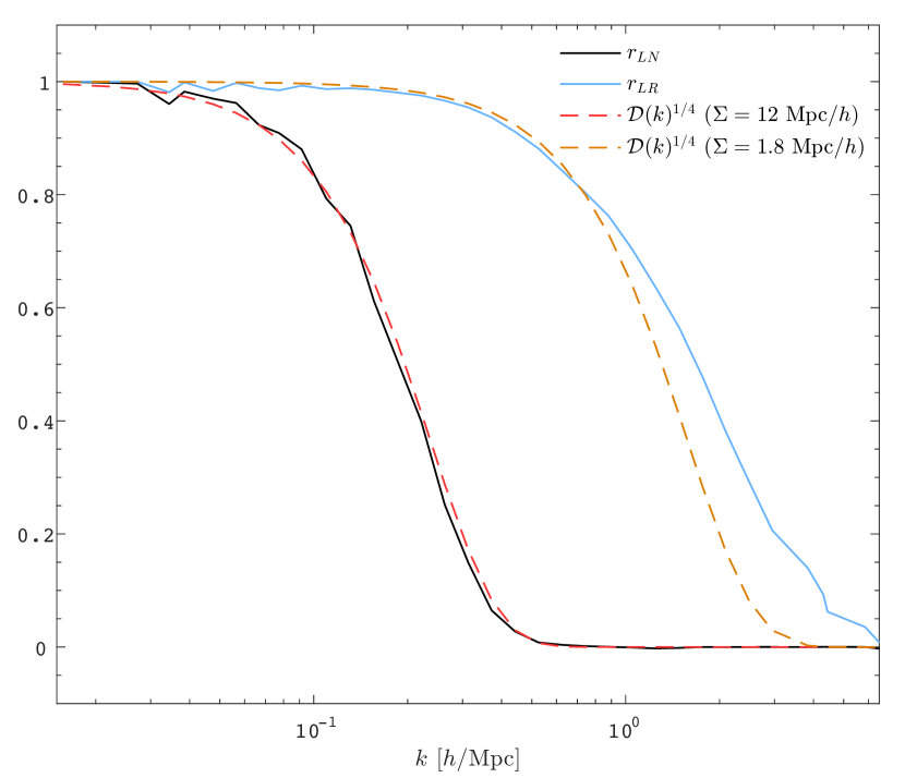
Figure 2: Correlation functions $r(\delta_{L},\delta_{N})$ and $r(\delta_{L},\delta_{R})$ (solid lines) and their scaled BAO damping models (dotted lines).

The two-point statistics of these density fields are quantified by the cross power spectrum $P_{ij}(k)\equiv(2\pi)^{-3}\langle|\delta_{i}(k)||\delta_{j}(k)|\rangle$, where subscripts $i,j$ may refer to linear ($L$), nonlinear ($N$), recovered ($R$), or noise ($n$) density fields. When $i=j$ it reduces to the auto power spectrum $P_{ii}(k)$ or $P(k)$. We usually plot the dimensionless power spectrum $\Delta^{2}(k)\equiv k^{3}P(k)/2\pi^{2}$.

II.2 Density recovery

In the simulation, we use particle-ID (PID) to record the initial (Lagrangian) location ${\boldsymbol{q}}$ of particles, and the information is tracked until the $z=0$ and we can get the Lagrangian displacement vector ${\boldsymbol{\Psi}}\equiv{\boldsymbol{x}}-{\boldsymbol{q}}$ for every particle. Then these vectors are interpolated onto the initial Lagrangian coordinates ${\boldsymbol{q}}$ of particles and we get the displacement field ${\boldsymbol{\Psi}}({\boldsymbol{q}})$. To visualize the $\boldsymbol{\Psi}$ field, we draw a 3D uniform mesh over the volume, and use the given $\boldsymbol{\Psi}$ field to deform the mesh according to the direction and physical amplitude of $\boldsymbol{\Psi}$. In the top panel of Fig.1, The resulting mesh illustrates a “pseudocurvilinear coordinate” similar to 1995ApJS..100..269P , however the mesh can be overlapped due to shell crossing. The densest mesh grids trace the densest structures of $\delta_{N}$, whereas the undeformed grid positions are the Lagrangian coordinates in which we do the density recovery. The raw recovered density field is given by the differential motion of matter elements,

$$\delta_{R}=-\nabla\cdot{\boldsymbol{\Psi}}({\boldsymbol{q}}).$$ (1)

Because the recovery processes are implemented on Lagrangian coordinates, $\delta_{R}$ takes the coordinates of $\boldsymbol{q}$ instead of $\boldsymbol{x}$. We just write $\boldsymbol{q}$’s Fourier wave number $k_{q}$ as $k$ to simplify the expression.

To quantify the linear information in the recovered density field $\delta_{R}$, we decompose $\delta_{L}$ in Fourier space into two uncorrelated parts,

$$\delta_{L}(k)=r^{\prime}\delta_{R}+\delta_{n},$$ (2)

where the first term $r^{\prime}\delta_{R}$ is completely correlated with $\delta_{R}$, meaning the linear information we can extract from $\delta_{R}$. The noise term $\delta_{n}$ is uncorrelated with $\delta_{R}$, being the rest of linear information which is not contained in $\delta_{R}$. Correlating equation (2) with $\delta_{R}$ gives

$$P_{LR}=r^{\prime}P_{RR}+P_{nR},$$ (3)

where $P_{ij}\equiv\langle\delta_{i}\delta_{j}\rangle$ denotes the cross power spectrum. Since $\delta_{n}$ is uncorrelated with $\delta_{R}$, $P_{nR}=0$. With the definition of cross correlation coefficient $r(\delta_{L},\delta_{R})\equiv P_{LR}/\sqrt{P_{LL}P_{RR}}$ and bias $b^{2}=P_{RR}/P_{LL}$, we solve $r^{\prime}=P_{LR}/P_{RR}=rb^{-1}$. Note that these computations above and below can also be applied on $\delta_{N}$ for comparison, by replacing “_R” with “_N” in the equations, while we do not rewrite them explicitly in the paper for simplicity. From these, we plot the cross correlation coefficient $r_{LN}=r(\delta_{L},\delta_{N})$ and $r_{LR}=r(\delta_{L},\delta_{R})$ in Fig.2. $r_{LN}$ shows no correlation starting from $k\simeq 0.4h/$Mpc (2004MNRAS.355..129S, ). Clearly, $\delta_{R}$ contains much more linear information on smaller scales.

According to equation (2), the auto power spectrum of $\delta_{L}$ is decomposed as

$$P_{LL}=r^{2}b^{-2}P_{RR}+P_{nn},$$ (4)

and $P_{nn}=(1-r^{2})P_{LL}$. We also explicitly compute the cross power spectrum between $\delta_{R}$ and $\delta_{n}=\delta_{L}-rb^{-1}\delta_{R}$, and found that $rb^{-1}P_{nR}$ is about two orders of magnitude lower than $P_{LL}$, being consistent with zero. This confirms that the signal term $rb^{-1}\delta_{R}$ and the noise term $\delta_{n}$ is indeed uncorrelated and validates equation (4). According to these two terms, we construct a Wiener filter to filter out the uncorrelated part in $\delta_{R}$:

$$W(k)=\frac{r^{2}b^{-2}P_{RR}}{r^{2}b^{-2}P_{RR}+P_{nn}}=r^{2}.$$ (5)

The optimal recovered density is given by

$$\tilde{\delta}_{R}=Wb^{-1}\delta_{R},$$ (6)

and the optimal recovered power spectrum is given by

$$\tilde{P}=W^{2}b^{-2}P_{RR}=W^{2}P_{LL}+W^{2}b^{-2}P_{NN}.$$ (7)

Here $W^{2}$ describes the damping of the linear power spectrum.

III Results

To visualize the above algorithms, a projection of $\delta_{R}$ is plotted in the bottom panel of Fig.1, which looks closer to $\delta_{L}$ compared to $\delta_{N}$. However the smallest scale structures are unable to be recovered.

As discussed in section II.2, Fig.2 shows the cross correlation functions $r_{LN}$ and $r_{LR}$. The latter extends the correlation with $\delta_{L}$ to smaller scales by nearly an order of magnitude. The extra correlation scales well cover the BAO scales of our interest.

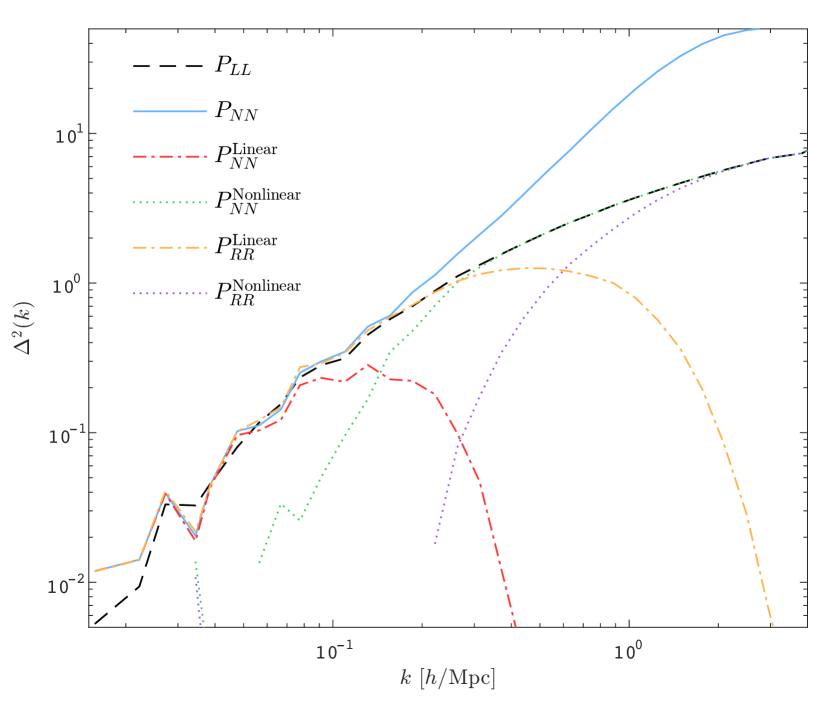
Figure 3: Power spectra of $\delta_{L}$, $\delta_{N}$, and the decomposition of $P_{LL}$ into correlated parts and noise terms according to equation (4).

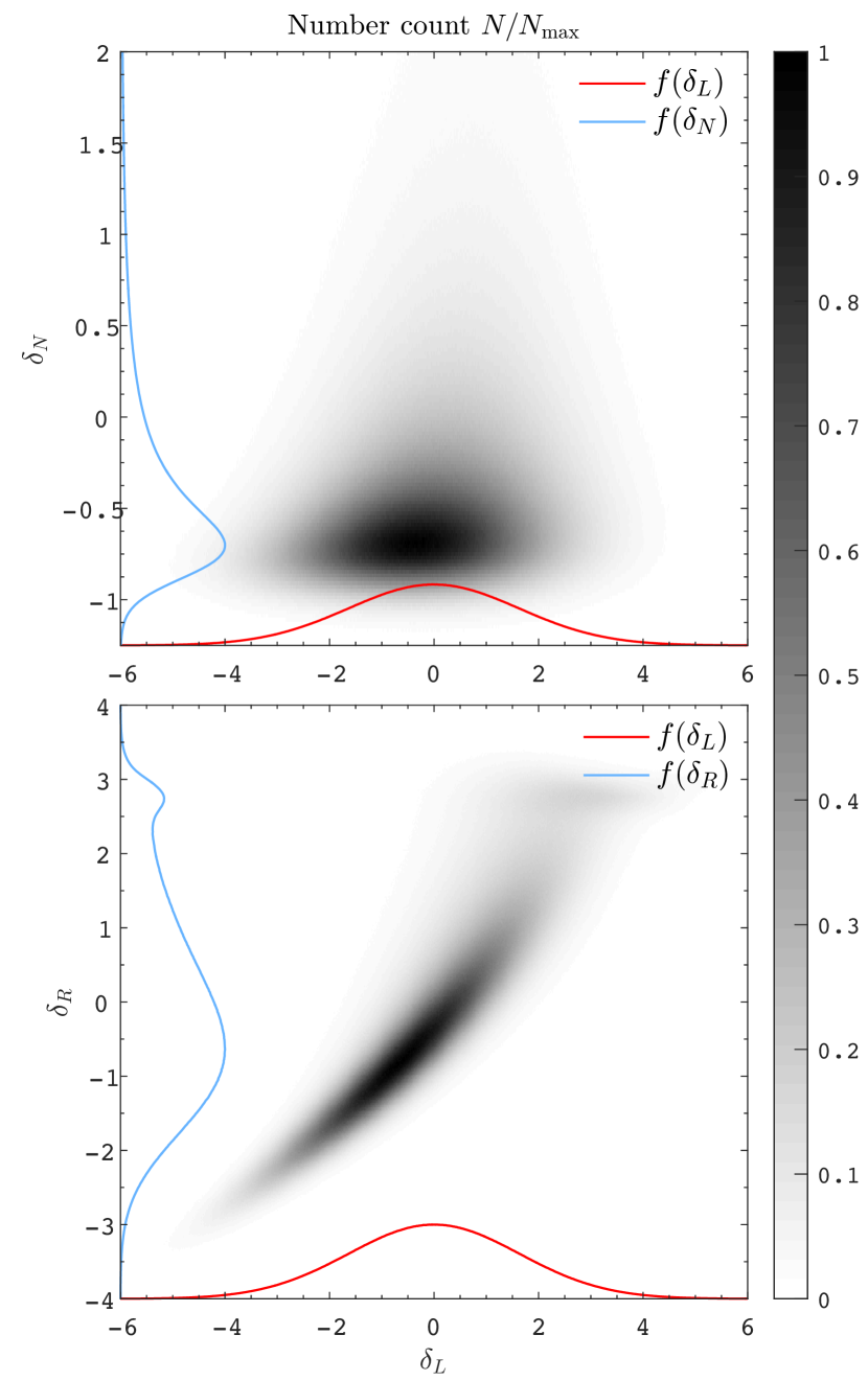
Figure 4: Probability distribution functions (PDFs) $f(\delta_{L},\delta_{N})$ and $f(\delta_{L},\delta_{R})$, showing in the upper and lower panels respectively. Both red curves on the $x$-axes show $f(\delta_{L})$, following a Gaussian distribution. The two curves on the $y$-axes in the upper and the lower panel show respectively $f(\delta_{N})$ and $f(\delta_{R})$.

In Fig.3, we show the auto power spectra of $\delta_{L}$ and $\delta_{N}$ in black dashed and blue solid curves. Their difference shows the nonlinear evolution of LSS on small scales. Their cross power (not shown for clarity of the figure) drops to a very low value on scales $k\gtrsim 0.1h/$Mpc, indicating a loss of linear information in the nonlinear power spectrum $P_{NN}$. This scenario directly leads to how $P_{LL}$ is decomposed according to equation (4). In nonlinear case (with “_R” replaced by “_N” equation (4)), on small scales $k\gtrsim 0.1h/$Mpc, $P_{LL}$ is dominated by uncorrelated, nonlinear noise, shown in the green dotted line. In the case of $\delta_{R}$, however, $P_{LL}$ is decomposed into the orange dash-dotted correlated part and the purple dotted uncorrelated part according to equation (4). The correlated power spectrum is dominated on BAO scales of our interest.

To quantify the improvement of cross-correlation in the power spectrum, we compute the damping factors $W^{2}(k)$ respectively for the optimal filtered nonlinear and recovered density fields $\tilde{\delta}_{N}$ and $\tilde{\delta}_{R}$. We fit Gaussian BAO damping models ${\mathcal{D}}(k)=\exp(-k^{2}\Sigma^{2}/2)$ to these $W^{2}(k)$’s and give $\Sigma=1.8$ Mpc$/h$ and $\Sigma=12$ Mpc$/h$ for $\delta_{R}$ and $\delta_{N}$. Since ${\mathcal{D}}(k)=W^{2}=r^{4}$, we plot ${\mathcal{D}}_{N}^{1/4}$ and ${\mathcal{D}}_{R}^{1/4}$ over $r_{LN}$ and $r_{LR}$ in Fig.2. The analyses are repeated with various box sizes (100, 300, 800 Mpc$/h$ per side) and give consistent results.

To further illustrate the improvement in real space one point function correlations, in Fig.4 we use the probability distribution as functions (PDFs) of $(\delta_{L},\delta_{N})$ and $(\delta_{L},\delta_{R})$ to show the point-point correlation between these two pairs of density fields. Since $\delta_{n}$ in equation (2) is uncorrelated, we use Wiener filtered fields. To keep the consistency over $\delta_{L}$, $\delta_{N}$ and $\delta_{R}$, we use the $W(k)=r^{2}_{LR}$ as the Wiener filter. The grey-scaled plots in the center of both panels show the two-variable PDFs, whereas their projections onto each variable are just one-variable PDFs – $f(\delta_{L})$, $f(\delta_{N})$ and $f(\delta_{R})$, shown as red/blue curves on the axes of Fig.4. In the top panel, $\delta_{N}$ shows an approximate log-normal distribution (blue curve) and $\delta_{L}$ follows an expected Gaussian distribution. They show tiny positive correlation in the 2D PDF. Because in Fourier space, $\delta_{L}$ and $\delta_{N}$ have correlations on only very large, linear scales (Fig.2), they result in little correlation in real space – initial density fluctuations in Lagrangian coordinates are evolved/transformed to Eulerian coordinates. As the recovery is done in Lagrangian space, it recovers certain amount of correlation, as shown in the 2D PDF of the bottom panel of Fig.4. One can also see that $\delta_{R}$ follows a much closer Gaussian distribution (blue curve of the bottom panel). In denser regions of $\delta_{L}$, $\delta_{R}$ is saturated at $\delta_{R}=3$, signifying the extreme collapsing of matter (2013MNRAS.428..141N, ): $\delta_{R}=-\nabla\cdot\boldsymbol{\Psi}=\nabla\cdot\boldsymbol{q}=3$. Shell crossing makes $\delta_{R}$ oscillate around 3. These second uncorrelated peaks damp out as we go to higher redshifts.

IV Discussion and conclusion

We extract the actual displacement field of matter elements in cosmological $N$-body simulations, and use this displacement field to study the LSS nonlinear clustering in Lagrangian space. The displacement information is used to recover the primordial linear perturbations. The result shows a prominent improvement from $r_{LN}$ to $r_{LR}$ in Fig.2 – recovering the lost linear information on nearly an order of magnitude smaller scales. This is achieved by implementing differential movement information of matter elements on Lagrangian coordinates, rather than on Eulerian coordinates. This result illustrates the feasibility of using estimated displacement field $\tilde{\boldsymbol{\Psi}}(\boldsymbol{q})$ to reconstruct primordial linear density field. A straightforward example of a estimation of $\tilde{\boldsymbol{\Psi}}(\boldsymbol{q})$ is given by 1995ApJS..100..269P ; 1998ApJS..115…19P . In reality, one needs to consider all aspects including vorticity, shell crossing, bias, noise and data complexities. The impact of these factors can be quantitatively compared with the impact of different estimation methods, and with the exact solution by $N$-body simulations.

The advantage of using displacement field in reconstruction is its insensitive response from highly nonlinearities. Nonlinear densities $\delta_{N}$ can be arbitrarily large – one expects virialized regions to be observable, where nonlinear density is given by the inverse determinant of the Jacobian $\delta_{N}=|\boldsymbol{J}|^{-1}\gtrsim 200$. However, reconstructed densities $\delta_{R}$ are given by the trace $\rm{tr}(\boldsymbol{J})$ and saturates at 3. Actually, the displacement fields are dominated by early stage linear processes, which is the Lagrangian-Eulerian coordinate transform, while late stage shell crossing, nonlinear and baryonic processes only fine-tune the final position $\boldsymbol{x}$ (2014PhRvD..89h3515C, ). Compared with estimated displacement fields $\tilde{\boldsymbol{\Psi}}(\boldsymbol{q})$ by 1995ApJS..100..269P , which do not have shell crossing, the additional shell crossing information in $\boldsymbol{\Psi}(\boldsymbol{q})$ is uncorrelated with $\delta_{L}$. This insensitive response from nonlinearities enables the stability of reconstruction algorithms, which are expected to give similar results of this paper. In contrast, traditional treatments in reconstruction deals directly on density fields which sensitively relies on nonlinear processes – density values can vary by orders of magnitude due to nonlinear/baryonic physics and many sources of errors.

References

- (1) Y. B. Zel’dovich, A&A5, 84 (1970).
- (2) M. Davis, G. Efstathiou, C. S. Frenk, and S. D. M. White, ApJ292, 371 (1985).
- (3) M. McQuinn and M. White, J. Cosmology Astropart. Phys1, 043 (2016), 1502.07389.
- (4) D. J. Eisenstein, New Astronomy Reviews 49, 360 (2005).
- (5) D. J. Eisenstein et al., ApJ633, 560 (2005), astro-ph/0501171.
- (6) W. Ngan, J. Harnois-Déraps, U.-L. Pen, P. McDonald, and I. MacDonald, MNRAS419, 2949 (2012), 1106.5548.
- (7) D. H. Weinberg, MNRAS254, 315 (1992).
- (8) J. Harnois-Déraps, H.-R. Yu, T.-J. Zhang, and U.-L. Pen, MNRAS436, 759 (2013), 1205.4989.
- (9) C. D. Rimes and A. J. S. Hamilton, MNRAS360, L82 (2005), astro-ph/0502081.
- (10) H.-R. Yu, J. Harnois-Déraps, T.-J. Zhang, and U.-L. Pen, MNRAS421, 832 (2012), 1012.0444.
- (11) D. J. Eisenstein, H.-J. Seo, E. Sirko, and D. N. Spergel, ApJ664, 675 (2007), astro-ph/0604362.
- (12) Y. Noh, M. White, and N. Padmanabhan, Phys. Rev. D80, 123501 (2009), 0909.1802.
- (13) N. Padmanabhan, M. White, and J. D. Cohn, Phys. Rev. D79, 063523 (2009), 0812.2905.
- (14) D. Jeong, Cosmology with high () redshift galaxy surveys, PhD thesis, University of Texas at Austin, 2010.
- (15) M. C. Neyrinck, MNRAS428, 141 (2013), 1204.1326.
- (16) K. C. Chan, Phys. Rev. D89, 083515 (2014), 1309.2243.
- (17) T. Baldauf, E. Schaan, and M. Zaldarriaga, J. Cosmology Astropart. Phys3, 017 (2016), 1505.07098.
- (18) U.-L. Pen, ApJS100, 269 (1995).
- (19) U.-L. Pen, ApJS115, 19 (1998), astro-ph/9704258.
- (20) H.-M. Zhu, U.-L. Pen, and X. Chen, ArXiv e-prints (2016), 1609.07041.
- (21) H. R. Yu and U.-L. Pen, (to be published) .
- (22) D. Blas, J. Lesgourgues, and T. Tram, J. Cosmology Astropart. Phys. 7, 034 (2011), 1104.2933.
- (23) R. W. Hockney and J. W. Eastwood, Computer simulation using particles (, 1988).
- (24) J. Harnois-Déraps et al., MNRAS436, 540 (2013), 1208.5098.
- (25) U. Seljak and M. S. Warren, MNRAS355, 129 (2004), astro-ph/0403698.