Iterative coupling of flow, geomechanics and adaptive phase-field fracture including level-set crack width approaches

Abstract

In this work, we present numerical studies of fixed-stress iterative coupling for solving flow and geomechanics with propagating fractures in a porous medium. Specifically, fracture propagations are described by employing a phase-field approach. The extension to fixed-stress splitting to propagating phase-field fractures and systematic investigation of its properties are important enhancements to existing studies. Moreover, we provide an accurate computation of the fracture opening using level-set approaches and a subsequent finite element interpolation of the width. The latter enters as fracture permeability into the pressure diffraction problem which is crucial for fluid filled fractures. Our developments are substantiated with several numerical tests that include comparisons of computational cost for iterative coupling and nonlinear and linear iterations as well as convergence studies in space and time.

1 Introduction

Iterative coupling has received great importance for coupling flow and mechanics in subsurface modeling, environmental and petroleum engineering problems [14, 23, 24, 41, 42, 52, 53]. Recently, the extension of iterative coupling to fractured porous media has been of interest [18, 43, 54]. However, reliable and efficient numerical methods in coupled poromechanics, including fractures, still pose computational challenges. The applications include multiscale and multiphysics phenomena such as reservoir deformation, surface subsidence, well stability, sand production, waste deposition, pore collapse, fault activation, hydraulic fracturing, CO₂ sequestration, and hydrocarbon recovery.

On the other hand, quasi-static brittle fracture propagation using variational techniques has attracted attention in recent years since the pioneering work in [10, 16]. The numerical approach [10] is based on Ambrosio-Tortorelli elliptic functionals [1, 2]. Here, discontinuities in the displacement field ${\bf u}$ across the lower-dimensional crack surface are approximated by an auxiliary function $\varphi$. This function can be viewed as an indicator function, which introduces a diffusive transition zone between the broken and the unbroken material. This zone has a half bandwidth $\varepsilon$, which is a model regularization parameter. From an application viewpoint, two situations are of interest for given fracture(s): first, observing the variation of the fracture width (crack opening displacement) and second, change of the fracture length. The latter situation is by far more complicated. However, both configurations are of importance and variational fracture techniques can be used for both of them.

Fracture evolutions satisfy a crack irreversibility constraint such that the resulting system can be characterized as a variational inequality. Our motivation for employing such a variational approach is that fracture nucleation, propagation, kinking, and the crack morphology are automatically included in the model. In addition, explicit remeshing or reconstruction of the crack path is not necessary. The underlying equations are based on principles arising from continuum mechanics that can be treated with (adaptive) Galerkin finite elements. An important modification of [16] towards a thermodynamically-consistent phase-field fracture model has been accomplished in [40, 36]. These approaches have been extended to pressurized fractures in [44, 45] that include a decoupled approach and a fully-coupled technique accompanied with rigorous analysis. Moreover, a free energy functional was established in [44]. In these last studies, the crack irreversibility constraint has been imposed through penalization. It it well-known that the energy functional of the basic displacement/phase-field model is non-convex and constitutes a crucial aspect in designing efficient and robust methods. Most approaches for coupling displacement and phase field are sequential, e.g., [11, 8, 13, 34]; however it is well-known that a monolithic treatment has higher robustness (and potentially better efficiency) than sequential coupling. Indeed it has been shown in [58, 17] that for certain phase-field fracture configurations partitioned coupling is more expensive than a monolithic solution. Consequently in this paper, we adopt a quasi-monolithic approach using an extrapolation in the phase-field variable [20, 30].

Recent advances and numerical studies for treating multiphysics phase-field fracture include the following; thermal shocks and thermo-elastic-plastic solids [12, 39, 35], elastic gelatin for wing crack formation [30], pressurized fractures [9, 45, 59, 61, 60], fluid-filled (i.e., hydraulic) fractures [43, 31, 38, 37, 33, 19, 63], proppant-filled fractures [29], a fractured well-model within a reservoir [62], and crack initiations with microseismic probability maps [32]. These studies demonstrate that phase-field fracture has great potential to tackle practical field problems.

Addressing multiphysics problems requires careful design of the solution algorithms. For the displacement/phase-field subproblem, we employ a quasi-monolithic approach as previously mentioned, but to couple this fractured-mechanics to flow, we use a splitting approach. The latter is more efficient for solvers and for choosing different time scales for both mechanics and flow, respectively. In addition, the splitting permits easier extensions to multiphase flow including equation of state (EOS) compositional flow. A successful splitting approach is fixed-stress iterative coupling, which has been applied in a series of papers for coupling phase-field fracture/mechanics and flow [43, 31, 29, 32]. However a systematic investigation of the performance of this scheme is still missing. It is the objective of this paper to illustrate using benchmarks and mesh refinement studies to establish the robustness and efficiency of the fixed-stress algorithm. These studies are essential for future extensions including efficient three-dimensional practical field problems.

In addition, we also focus on a more accurate approximation of the fracture width. The authors of [46] recently proposed a two-stage level-set approach in which first a level-set function is computed with the help of the phase-field function and in a second step this level-set function is smoothed due to high gradients. However, since we only need the level-set function to obtain normal vectors on the fracture boundary, we also propose an alternative method which simplifies the above approach by avoiding the computation of an explicit level-set function but directly using the computed phase-field function. In addition, we note that these approaches do not derive the width formulation inside the fracture, which is crucial for the fracture permeability computation for fluid filled fracture propagations. Thus, here we propose a method to compute the crack width values inside the fracture by employing an interpolation based on the values in the diffusive fracture zone.

To resulting fluid filled fracture propagation framework consists of five equations (four equations when using phase-field directly as a level-set value) for five (i.e., four) unknowns: vector-valued displacements ${\bf u}$, scalar-valued phase-field $\varphi$, pressure $p$, level-set $\varphi_{\textsf{LS}}$, and a finite element representation of the fracture width $w$. The first problem (namely the displacement/phase-field) is nonlinear and subject to an inequality constraint-in-time (the crack irreversibility) whereas the other three problems are linear.

The outline of this paper is as follows: In Section 2 we recapitulate the flow equations in terms of a pressure diffraction problem, and the displacement-phase-field system for the mechanics part. In Section 3, two equations for computing a level-set function and the width are formulated. In Section 4 we discuss the discretization of all problems. In the next Section 5 we address discretization and the fixed-stress coupling algorithm. Several numerical examples are presented in Section 6, which demonstrate the performance of our algorithmic developments.

2 Mathematical models for flow and mechanics of porous media and fractures

2.1 Preliminaries

Let $\Lambda\in\mathbb{R}^{d}$, $d=2,3$ be a smooth open and bounded computational domain with Lipschitz boundary $\partial\Lambda$ and let $[0,T]$ be the computational time interval with $T>0$. We assume that the crack $\mathcal{C}$ is contained in $\Lambda$. The prototype configuration for a horizontal penny shape fracture is given in Figure 1. Here, we emphasize that the crack is seen as a thin three-dimensional volume $\Omega_{F}(t)$ using $\varepsilon$ at time $t\in[0,T]$ (see Figure 2), where the thickness is much larger than the pore size of the porous medium. The boundary of the fracture is denoted by $\Gamma_{F}(t):=\bar{\Omega}_{F}(t)\cap\bar{\Omega}_{R}(t)$, where $\Omega_{R}:=\Lambda\setminus\Omega_{F}$ represents the porous media.

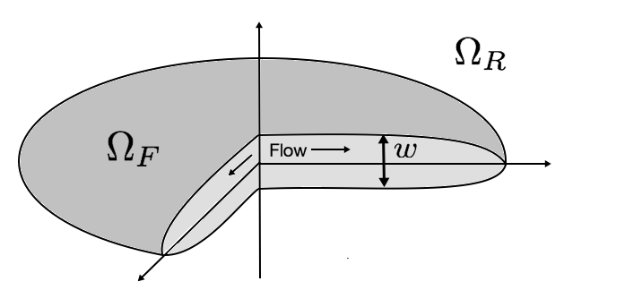
Figure 1: Sketch of a penny shaped fracture region ($\mathcal{C}$) for a three-dimensional setting. The fracture boundary moves in time.

Throughout the paper, we will use the standard notation for Sobolev spaces and their norms. For example, let $E\subseteq\Lambda$, then $\|\cdot\|_{1,E}$ and $|\cdot|_{1,E}$ denote the $H^{1}(E)$ norm and semi-norm, respectively. The $L^{2}(E)$ inner product is defined as $(f,g):=\int_{E}fg\ d{\bf x}$ for all $v,w\in L^{2}(E)$ with the norm $\|\cdot\|_{E}$. For simplicity, we eliminate the subscripts on the norms if $E=\Lambda$. For any vector space ${\bf X}$, ${\bf X}^{d}$ will denote the vector space of size $d$, whose components belong to ${\bf X}$ and ${\bf X}^{d\times d}$ will denote the $d\times d$ matrix whose components belong to ${\bf X}$.

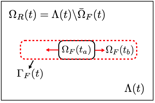
(a)

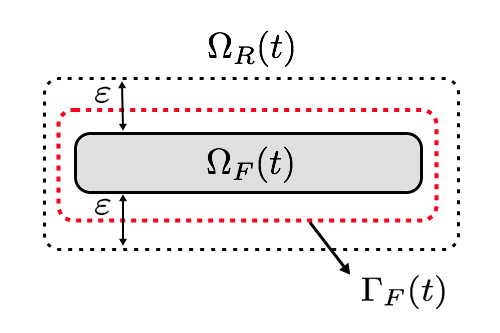
(b)

Figure 2: Sketch of the (a) time dependent domain for a propagating fracture for two different times $t_{a}<t_{b}$ and (b) a fixed fracture with the transition zone where the width is $\varepsilon$.

2.2 A pressure diffraction flow system

We now formulate the flow problem in terms of a diffraction system [26]. Specifically, the underlying Darcy flow equations have the same structure in both the porous medium and the fracture. Using varying coefficients and an indicator variable allows to distinguish between reservoir flow and fracture flow.

To derive the flow pressure equations for each sub-domain, first we consider the two separate mass continuity equations for the fluid in the reservoir and the fracture, which we can rewrite as

$$\partial_{t}(\rho_{F}\varphi^{\star}_{F})+\nabla\cdot(\rho_{F}{\bf v}_{F}) =q_{F}-q_{L} \text{in }\quad\Omega_{F}\times(0,T],$$ (1)

$$\partial_{t}(\rho_{R}\varphi^{\star}_{R})+\nabla\cdot(\rho_{R}{\bf v}_{R}) =q_{R} \text{in }\quad\Omega_{R}\times(0,T].$$ (2)

Here $\rho_{F}$, $\rho_{R}$ are fluid densities, $q_{L}$ is a leak-off term (which is assumed to be zero in the following), $q_{F}$ and $q_{R}$ are source/sink terms for fracture and reservoir, respectively.

We assume the fluid in the reservoir ($j=R$) and the fracture ($j=F$) is slightly compressible, thus we define the fluid density as

$$\rho_{j}:=\rho_{j}^{0}\exp(c_{j}(p_{j}-p_{j}^{0}))\approx\rho_{j}^{0}[1+c_{j}(p_{j}-p_{j}^{0})],\ j\in\{F,R\}$$ (3)

where $p_{j}:\Omega_{j}\times[0,T]\rightarrow\mathbb{R}$ is the pressure, $p_{0}$ is the initial pressure at $t=0$, $\rho_{j}^{0}$ is the reference density and $c_{j}$ is the fluid compressibility. In addition, $\varphi^{\star}_{R}$ and $\varphi^{\star}_{F}$ are the reservoir and fracture fluid fraction respectively and we set $\varphi^{\star}_{F}=1$ (since the porosity of the fracture is assumed to be one) and

$$\varphi_{R}^{\star}:=\varphi^{\star}_{0}+\alpha\nabla\cdot{\bf u}+\dfrac{1}{M}(p_{R}-p_{0}).$$ (4)

Here ${\bf u}:\Omega\times[0,T]\rightarrow\mathbb{R}^{d}$ is the solid displacement, $\alpha\in[0,1]$ is the Biot coefficient, $M>0$ is a given Biot modulus, and $\varphi^{\star}_{0}$ is the initial value.

Next, we describe the flow given by Darcy’s law for the fracture and for the reservoir , respectively by

$${\bf v}_{j}=-\dfrac{K_{j}}{\eta_{j}}(\nabla p_{j}-\rho_{j}{\bf g}),\ j\in\{F,R\}$$ (5)

where $\eta_{j}$ is the fluid viscosity, $K_{j}$ is the permeability, and ${\bf g}$ is the gravity.

Following the general reservoir approximation with the assumption that $c_{R}$ and $c_{F}$ are small enough, we use $\rho_{R}=\rho_{R}^{0}$ and $\rho_{F}=\rho_{F}^{0}$, and assume $p_{0}=0$, to rewrite the equations (1)-(2) by

$$\rho_{R}^{0}\partial_{t}(\dfrac{1}{M}p_{R}+\alpha\nabla\cdot{\bf u})-\nabla\cdot\dfrac{K_{R}\rho_{R}^{0}}{\eta_{R}}(\nabla p_{R}-\rho_{R}^{0}{\bf g})=q_{R} \text{in }\quad\Omega_{R}\times(0,T],$$ (6)

$$\rho_{F}^{0}c_{F}\partial_{t}p_{F}-\nabla\cdot\dfrac{K_{F}\rho_{F}^{0}}{\eta_{F}}(\nabla p_{F}-\rho_{F}^{0}{\bf g})=q_{F} \text{in }\quad\Omega_{F}\times(0,T].$$ (7)

Inside the fracture flow equation, the fracture permeability is assumed to be isotropic such that

$$K_{F}=\frac{1}{12}w({\bf u})^{2},$$ (8)

where $w({\bf u})=[{\bf u}\cdot{\bf n}]$ denotes the aperture (width) of the fracture, which means that the jump $[\cdot]$ of normal displacements has to be computed; corresponding details are provided in Section 3. For further non-isotropic lubrication laws that have been specifically derived for fluid-filled phase-field fractures, we refer to [43, 29].

The system is supplemented with initial and boundary conditions. The initial conditions for the pressure diffraction equations (6)-(7) are given by:

$$p_{F}({\bf x},0) =p_{F}^{0}\quad\text{for all }{\bf x}\in\Omega_{F}(t=0),$$

$$p_{R}({\bf x},0) =p_{R}^{0}\quad\text{for all }{\bf x}\in\Omega_{R}(t=0),$$

where $p_{F}^{0}$ and $p_{R}^{0}$ are smooth given pressures. Also we have

$$\varphi({\bf x},0)=\varphi^{0}\quad\text{for all }{\bf x}\in\Lambda(t=0),$$

where $\varphi^{0}$ is a given smooth initial fracture.

We prescribe the boundary and interface conditions for pressure as

$$K_{R}(\nabla p_{R}-\rho_{R}^{0}{\bf g})\cdot{\bf n} =0 \text{on}\quad\partial\Lambda\times(0,T],$$ (9)

$$[p] =0 \text{on }\hskip 16.62178pt\Gamma_{F}\times(0,T],$$ (10)

$$\dfrac{K_{R}\rho_{R}^{0}}{\eta_{R}}(\nabla p_{R}-\rho_{R}^{0}{\bf g})\cdot{\bf n} =\dfrac{K_{F}\rho_{F}^{0}}{\eta_{F}}(\nabla p_{F}-\rho_{F}^{0}{\bf g})\cdot{\bf n} \text{on }\hskip 16.62178pt\Gamma_{F}\times(0,T],$$ (11)

where ${\bf n}$ is the outward pointing unit normal on $\Gamma_{F}$ or $\partial\Lambda$.

In order to finalize our derivation we perform two steps; first, we introduce the coefficients with indicator functions to combine equations (6) and (7), secondly, we formulate the weak form in terms of a pressure diffraction system. The weak formulation reads:

Formulation 1.

Find $p(\cdot,t)\in V_{p}=H^{1}(\Lambda)$ for almost all times $t\in(0,T]$ such that,

$$\rho_{0}(\partial_{t}{\varphi^{\star}},v)+({\rho_{0}K_{eff}}(\nabla p-\rho_{0}{\bf g}),\nabla v)-(q,v)=0,\quad\forall v\in V_{p}$$ (12)

where the coefficient functions are defined as

$$\rho_{0} =\chi_{\Omega_{R}}\rho_{R}^{0}+\chi_{\Omega_{F}}\rho_{F}^{0},$$ (13)

$${\varphi^{\star}} ={\varphi^{\star}}(\cdot,t):=\chi_{\Omega_{R}}\Bigl{(}\dfrac{1}{M}p_{R}+\alpha\nabla\cdot{\bf u}\Bigr{)}+\chi_{\Omega_{F}}(c_{F}p_{F}),$$ (14)

$${q} =q(\cdot,t):=\chi_{\Omega_{R}}{q_{R}}+\chi_{\Omega_{F}}q_{F},$$ (15)

$$K_{eff} :=\chi_{\Omega_{R}}\dfrac{K_{R}}{\eta_{R}}+\chi_{\Omega_{F}}\dfrac{K_{F}}{\eta_{F}},$$ (16)

where $\chi_{\Omega_{R}}=1$ and $\chi_{\Omega_{F}}=0$ in $\Omega_{R}$, and $\chi_{\Omega_{R}}=0$ and $\chi_{\Omega_{F}}=1$ in $\Omega_{F}$ .

2.3 Geomechanics and phase-field fracture equations

The displacement of the solid and diffusive flow in a non-fractured porous medium are modeled in $\Omega_{R}$ by the classical quasi-static elliptic-parabolic Biot system for a porous solid saturated with a slightly compressible viscous fluid. The constitutive equation for the Cauchy stress tensor is given as

$$\sigma^{por}({\bf u},p)-\sigma_{0}=\sigma({\bf u})-\alpha(p-p_{0})I,$$ (17)

where $I$ is the identity tensor and $\sigma_{0}$ is the initial stress value. The effective linear elastic stress tensor is

$$\sigma:=\sigma({\bf u})=\lambda(\nabla\cdot{\bf u})I+2Ge({\bf u}),$$ (18)

where $\lambda,G>0$ are the Lamé coefficients. The linear elastic strain tensor is given as $e({\bf u}):=\frac{1}{2}(\nabla{\bf u}+\nabla{\bf u}^{T})$. Then the balance of linear momentum in the solid reads

$$-\nabla\cdot\sigma^{por}({\bf u},p)=\rho_{s}{\bf g}\quad\text{in }\Omega_{R}\times(0,T],$$ (19)

where $\rho_{s}$ is the density of the solid. We prescribe homogeneous Dirichlet boundary conditions on $\partial\Lambda$ for the displacement ${\bf u}$.

In the following, we describe our fracture approach in a porous medium using the previous setup. Modeling fractures with a phase-field approach in $\Lambda$ is formulated with the help of an elliptic (Ambrosio-Tortorelli) functional [1, 2] and a variational setting, which has been first proposed for linear elasticity in [16, 10].

We now recapitulate the essential elements for a phase-field model for pressurized and fluid filled fractures in porous media, which has been modeled in [44, 45] including rigorous analysis. Two unknown solution variables are sought, namely vector-valued displacements ${\bf u}(\cdot,t)$ and a smoothed scalar-valued indicator phase-field function $\varphi(\cdot,t)$. Here $\varphi=0$ denotes the crack region ($\Omega_{F}$) and $\varphi=1$ characterizes the unbroken material ($\Omega_{R}$). The intermediate values constitute a smooth transition zone dependent on a regularization parameter $\varepsilon>0$.

The physics of the underlying problem requires a crack irreversibility condition that is an inequality condition in time:

$$\partial_{t}\varphi\leq 0.$$ (20)

Consequently, modeling of fracture evolution problems leads to a variational inequality system, that is always, due to this constraint, quasi-stationary or time-dependent.

The resulting variational formulation is stated in an incremental (i.e., time-discretized) formulation in which the continuous irreversibility constraint is approximated by

$$\varphi\leq\varphi^{old}.$$

Here, $\varphi^{old}$ will later denote the previous time step solution and $\varphi$ the current solution. Let the function spaces be given by $V:=H^{1}_{0}(\Lambda),W:=H^{1}(\Lambda)$ and

$$W_{in}:=\{w\in H^{1}(\Lambda)|\,w\leq\varphi^{old}\leq 1\text{ a.e. on }\Lambda\}.$$

We note that the phase field function is subject to homogeneous Neumann conditions on $\partial\Lambda$. The Euler-Lagrange system for pressurized phase-field fracture reads [45]:

Formulation 2.

Let $p\in H^{1}(\Lambda)$ be given. Find $\{{\bf u},\varphi\}\in V\times W$ such that

$$\Bigl{(}\big{(}(1-\kappa){\varphi}^{2}+\kappa\big{)}\;\sigma^{+}({\bf u}),e({{\bf w}})\Bigr{)}+(\sigma^{-}({\bf u}),e({\bf w}))$$ (21)

$$\quad-(\alpha-1)({\varphi}^{2}p,\mbox{div }{{\bf w}})+({\varphi}^{2}\nabla p,{{\bf w}})=0\quad\forall{\bf w}\in V,$$

and

$$(1-\kappa)({\varphi}\;\sigma^{+}({\bf u}):e({\bf u}),\psi{-\varphi})-2(\alpha-1)({\varphi}\;p\;\mbox{div }{\bf u},\psi{-\varphi})+2\,({\varphi}\nabla p\;{u},\psi)$$ (22)

$$+G_{c}\Bigl{(}-\frac{1}{\varepsilon}(1-\varphi,\psi{-\varphi})+\varepsilon(\nabla\varphi,\nabla(\psi-{\varphi}))\Bigr{)}\geq 0\quad\forall\psi\in W_{in}\cap L^{\infty}(\Lambda).$$

Here, $G_{c}$ is the critical energy release rate and $\kappa$ is a very small positive regularization parameter ($\kappa\approx 0$) for the elastic energy (in some cases, see for instance [7], $\kappa=0$ even works). Physically, $\kappa$ represents the residual stiffness of the material. Consequently, since

$$\big{(}(1-\kappa){\varphi}^{2}+\kappa\big{)}\;\rightarrow\kappa\quad\text{for }\varphi\to 0,$$

the material stiffness decreases while approaching the fracture zone. Regarding the stress tensor split, we follow [3] in which the stress tensor is additively decomposed into a tensile part $\sigma^{+}({\bf u})$ and a compressive part $\sigma^{-}({\bf u})$ by:

$$\sigma^{+}({\bf u}) :=(\dfrac{2}{n}G+\lambda)tr^{+}(e({\bf u}))I+2G(e({\bf u})-\dfrac{1}{n}tr(e({\bf u}))I),$$ (23)

$$\sigma^{-}({\bf u}) :=(\dfrac{2}{n}G+\lambda)tr^{-}(e({\bf u}))I,$$ (24)

where $n$ is the dimension (2 or 3) and

$$tr^{+}(e({\bf u}))=\max(tr(e({\bf u})),0),\quad tr^{-}(e({\bf u}))=tr(e({\bf u}))-tr^{+}(e({\bf u})).$$ (25)

We emphasize that the energy degradation only acts on the tensile part.

3 The fracture width computation using a level-set approach

A crucial issue in fluid-filled fractures is the fracture width $w:=w({\bf u})$ computation since this enters as fracture permeability values (8) into the pressure diffraction problem. Previously, the fracture width was approximated by given point values of displacements in [31, 29] and a method for a single fracture constructing an additional displacement field was studied in [57]. In this section, we introduce a computational method to compute the crack width more robustly, especially inside the fracture.

The first challenge is to compute the normal vector of the fracture interface. Here the method is inspired by a recent idea proposed in [46] by introducing an (explicit) level-set function $\varphi_{\textsf{LS}}$ for the fracture. However, we also note that employing a level-set function to compute the normal vectors of iso-surfaces has been used for many different applications (for example, see [22, 6] and references cited therein). The initial step follows a standard procedure in level-set methods. Let $\Gamma_{F}$ be the fracture boundary. We now define $\Gamma_{F}$ as the zero levels-set of a function $\varphi_{\textsf{LS}}$ such that

$$\varphi_{\textsf{LS}} >0,\quad{\bf x}\in\Omega_{R},$$

$$\varphi_{\textsf{LS}} <0,\quad{\bf x}\in\Omega_{F},$$

$$\varphi_{\textsf{LS}} =0,\quad{\bf x}\in\Gamma_{F},$$

where $\Gamma_{F}:=\{{\bf x}\in\Lambda\ |\ \varphi({\bf x},t)={C_{LS}}\}$, $\Omega_{R}:=\{{\bf x}\in\Lambda\ |\ \varphi({\bf x},t)>C_{LS}\}$ and $\Omega_{F}:=\{{\bf x}\in\Lambda\ |\ \varphi({\bf x},t)<C_{LS}\}$. Here $C_{LS}\in(0,1)$ is a constant that we have to choose to define the fracture boundary $\Gamma_{F}$, since the phase field approach involves the diffusion zone between $\Omega_{R}$ and $\Omega_{F}$ with length $\varepsilon$ (see Figure 2). However, since $\varepsilon$ is very small and the dependency of the choice of $C_{LS}$ is minimal (e.g [31]), we set $C_{LS}=0.1$ throughout this paper for simplicity. In the following, we propose two different methods to compute $\varphi_{\textsf{LS}}$, where one (Formulation 3) is a similar technique as shown in [46].

Formulation 3 (Level-set values obtained by computing an additional problem).

Find $\varphi_{\textsf{LS}}$ such that

$$-\Delta\varphi_{\textsf{LS}} =f_{\textsf{LS}}(\cdot,t)\quad\text{in }\Lambda,$$ (26)

$$\varphi_{\textsf{LS}} =0\quad\text{on }\Gamma_{F},$$ (27)

$$\partial_{{\bf n}}\varphi_{\textsf{LS}} =0\quad\text{on }\partial\Lambda,$$ (28)

where

$$f_{\textsf{LS}}(\cdot,t)=\chi(\cdot,t)f_{1}+(1-\chi(\cdot,t))f_{2}$$

with $\chi(\cdot,t)=0$ for $\varphi({\bf x},t)<C_{LS}$ and $\chi(\cdot,t)=1$ otherwise. For simplicity, we set $f_{1}=-10$ and $f_{2}=10$.

Figure 3 illustrates the result for the level-set formulation with a simple fracture in the middle of the domain.

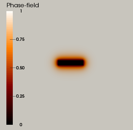
(a) Phase field $\varphi$.

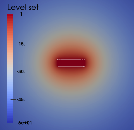
(b) Level-set $\varphi_{\textsf{LS}}$

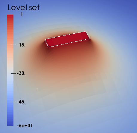
(c) Level-set $\varphi_{\textsf{LS}}$

Figure 3: For a given fracture in the middle of domain, (a) the phase field values and in (b)-(c) the level-set values with zero level-set ($\varphi_{\textsf{LS}}=0)$ are illustrated. In (c), a three-dimensional surface plot is shown.

The other alternative approach differs from Formulation 3 is to directly using the phase-field values by shifting them but without solving an additional problem:

Formulation 4 (Level-set values obtained from phase-field).

As second alternative approach, the level-set values are immediately obtained from the phase-field by:

$$\varphi_{\textsf{LS}}=\varphi-C_{LS}.$$

Remark 1 (Regularity properties of $\varphi_{\textsf{LS}}$).

Exemplarily, we refer to [22, section 4.5] for discussions regarding to the regularity properties of $\varphi_{\textsf{LS}}$ and to improve the accuracy for computing the gradients across the $\Gamma_{F}$.

Next, with the computed level-set value $\varphi_{\textsf{LS}}$ (either obtained from Formulation 3 or 4), we obtain the outward normal vector for a given level-set fracture boundary by the following procedure:

Formulation 5 (Computing the width with the normal vector on the fracture boundary).

Under the assumption that ${\bf u}^{+}\cdot{\bf n}=-{\bf u}^{-}\cdot{\bf n}$ (symmetric displacements at the fracture boundary), we compute the width locally in each quadrature point

$$w_{D}:=2{\bf u}\cdot{\bf n}_{F}=-2{\bf u}\cdot\frac{\nabla\varphi_{\textsf{LS}}}{\|\nabla\varphi_{\textsf{LS}}\|}\quad\text{on }\Gamma_{F}.$$ (29)

Here we assume that ${\bf u}^{+}\cdot{\bf n}=-{\bf u}^{-}\cdot{\bf n}$, which has been justified for tensile stresses and homogeneous isotropic media. These results are compatible for fluid filled fracture as we observe in our computational results, e.g., see Figure 7, in comparison to just taking two times the ${\bf u}_{y}$ displacements.

The second challenge is to compute the width values inside the crack, which is required for the permeability in fluid filled fracture propagation, see (8). Here we propose a method, Formulation 6, to compute the crack width values inside the fracture by employing an interpolation based on the values on $\Gamma_{F}$.

Formulation 6 (Crack width interpolation inside the fracture).

We solve the following width-problem: Find $w\in H^{1}$ such that

$$-\Delta w =g\quad\text{in }\Lambda,$$

$$w =w_{D}\quad\text{on }\Gamma_{F},$$ (30)

$$w =0\quad\text{on }\partial\Lambda.$$

Here $g({\bf x})=\beta\|w\|_{L^{\infty}(\Lambda)}$, where $\beta\approx 100$, in order to obtain a smooth parabola-type width-profile in the fracture. We note that $\beta$ is problem-dependent and heuristically chosen. In the case of multiple fractures, say $m$ fractures, we determine a locally highest width, where $\|w\|_{L^{\infty}(\Lambda_{l})},\ l\in\{1,\cdots,m\}$ is defined on the local region near the fracture such that $\Lambda:=\Lambda_{1}\cup\Lambda_{2}\cup\cdots\cup\Lambda_{m}$.

Figure 4 illustrates the result for Formulations 3-6 with crack width in the fracture. Finally we can approximate accurate crack width values in the fracture.

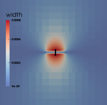
(a) $w_{D}$ by (29).

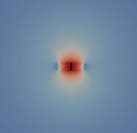
(b) $w$ by (30).

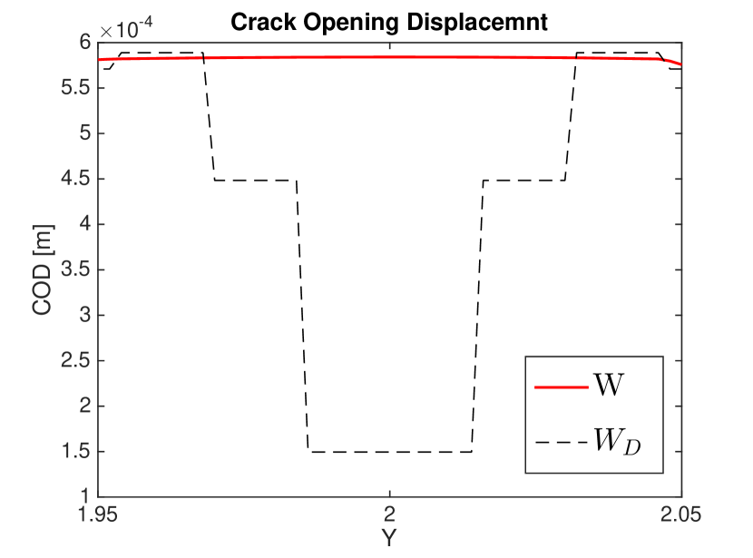
(c) Comparison.

Figure 4: In (a), we visualize a fracture width evaluation by employing (29) for the phase field fracture and the level-set given in Figure 3. The fracture width is computed correctly up to the fracture boundary. However, in the very inner of the fracture $\varphi\simeq 0$, all values are nearly zero. Then, (b) we compute the width in each quadrature point and finally solve a width-problem (30) in order to interpolate the fracture-boundary width values inside the fracture. (c) shows the comparison between (a) and (b) over the middle line $y-$direction illustrated in the fracture.

Remark 2.

Using Formulation 3 for computing the width is accompanied by the cost that we need to solve two additional problems. However, we emphasize that in our algorithm these two subproblems are scalar-valued, linear, and elliptic and therefore much cheaper to compute in comparison to the other subproblems. The advantage of this procedure being that we have an accurate width computation as well as a representation of a global finite element function that can be easily accessed in the program. In addition, the above computation can be employed for multiple non-planar fractures. To further reduce the computational cost Formulation 3 and can be replaced by Formulation 4.

4 Discretization of all sub-systems

In this section, we first address discretization of the pressure flow system and then we consider the displacement-phase-field system. Finally, we provide the variational formulations of the discrete level-set and width problems. We consider a mesh family $\{\mathcal{T}_{h}\}_{h>0}$, which is assumed to be shape regular in the sense of Ciarlet, and we assume that each mesh $\mathcal{T}_{h}$ is a subdivision of $\bar{\Lambda}$ made of disjoint elements $\mathcal{K}$, i.e., squares when $d=2$ or cubes when $d=3$. Each subdivision is assumed to exactly approximate the computational domain, thus $\bar{\Lambda}=\cup_{K\in\mathcal{T}_{h}}\mathcal{K}$. The diameter of an element $\mathcal{K}\in\mathcal{T}_{h}$ is denoted by $h$ and we denote $h_{\min}$ for the minimum. For any integer $k\geq 1$ and any $\mathcal{K}\in\mathcal{T}_{h}$, we denote by $\mathbb{Q}^{k}(\mathcal{K})$ the space of scalar-valued multivariate polynomials over $\mathcal{K}$ of partial degree of at most $k$. The vector-valued counterpart of $\mathbb{Q}^{k}(\mathcal{K})$ is denoted $\boldsymbol{\mathbb{Q}}^{k}(\mathcal{K})$. We define a partition of the time interval $0=:t^{0}<t^{1}<\cdots<t^{N}:=T$ and denote the time step size by $\delta t:=t^{n}-t^{n-1}$.

4.1 Decomposing the domain $\Lambda$ into $\Omega_{R}$ and $\Omega_{F}$

(a)

(b)

Figure 5: (a) The linear indicator functions $\chi_{F}$ and $\chi_{R}$ illustrated with adjustable constants $c_{1}$ and $c_{2}$. (b) We consider as the fracture zone if $\varphi\leq c_{1}$ and as the reservoir zone if $\varphi\geq c_{2}$.

We define the fracture domain $\Omega_{F}$ and the reservoir domain $\Omega_{R}$ by introducing two linear indicator functions $\chi_{F}$ and $\chi_{R}$ for the two different sub-domains; they satisfy

$$\chi_{R}(\cdot,\varphi) :=\chi_{R}({\bf x},t,\varphi)=1\quad\text{in }\quad\Omega_{R}(t),\quad\text{and }\quad\chi_{R}(\cdot,\varphi)=0\quad\text{in }\quad\Omega_{F}(t),$$ (31)

$$\chi_{F}(\cdot,\varphi) :=\chi_{F}({\bf x},t,\varphi)=1\quad\text{in }\quad\Omega_{F}(t),\quad\text{and }\quad\chi_{F}(\cdot,\varphi)=0\quad\text{in }\quad\Omega_{R}(t).$$ (32)

Thus $\chi_{F}(\cdot,\varphi)$ is zero in the reservoir domain and $\chi_{R}(\cdot,\varphi)$ is zero in the fracture domain. In the diffusive zone, the linear functions are defined as

$$\chi_{F}(\cdot,\varphi)=-\dfrac{(\varphi-c_{2})}{(c_{2}-c_{1})}\quad\text{and}\quad\chi_{R}(\cdot,\varphi)=\dfrac{(\varphi-c_{1})}{(c_{2}-c_{1})}.$$ (33)

Thus $\chi_{R}(\cdot,\varphi)=0$ and $\chi_{F}(\cdot,\varphi)=1$ if $\varphi({\bf x},t)\leq c_{1}$, and $\chi_{R}(\cdot,\varphi)=1$ and $\chi_{F}(\cdot,\varphi)=0$ if $\varphi({\bf x},t)\geq c_{2}$, where $c_{1}:=0.5-c_{x}$ and $c_{2}=0.5+c_{x}$. For simplicity we set $c_{x}=0.1$.

4.2 Temporal and spatial discretization of the pressure diffraction equation

The space approximation $P$ of the pressure function $p({\bf x},t)$ is approximated by using continuous piecewise polynomials given in the finite element space,

$$\mathbb{W}(\mathcal{T}):=\{W\in C^{0}(\bar{\Lambda};\mathbb{R})\ |\ W|_{\mathcal{K}}\in\mathbb{Q}^{1}(\mathcal{K}),\forall\mathcal{K}\in\mathcal{T}\}.$$ (34)

Note that we employ enriched Galerkin approximation [28] when we couple with transport problem which requires local and global conservation for flux [29].

Assuming that the displacement field ${\bf u}$ and the phase field $\varphi$ are known, the Galerkin approximation of (6)-(7) is formulated as follows. Given $P({\bf x},0)=P^{0}$ where $P^{0}$ is an approximation of the initial condition $p^{0}$, find $P\in C^{1}([0,T];\mathbb{W}(\mathcal{T}))$ such that

$$\chi_{R}(\cdot,\varphi)\Biggl{(}\int_{\Lambda}\rho_{R}^{0}\partial_{t}(\dfrac{1}{M}P+\alpha\nabla\cdot{\bf u})\omega\ d{\bf x}+\int_{\Lambda}\dfrac{K_{R}\rho_{R}^{0}}{\eta_{R}}(\nabla P-\rho_{R}^{0}{\bf g})\nabla\omega\ d{\bf x}=\int_{\Lambda}q_{R}\omega\ d{\bf x}\Biggr{)},\quad\forall\omega\in\mathbb{W}(\mathcal{T}),$$ (35)

$$\chi_{F}(\cdot,\varphi)\Biggl{(}\int_{\Lambda}\rho_{F}^{0}c_{F}\partial_{t}P\omega\ d{\bf x}+\int_{\Lambda}\dfrac{K_{F}\rho_{F}^{0}}{\eta_{F}}(\nabla P-\rho_{F}^{0}{\bf g})\nabla\omega\ d{\bf x}=\int_{\Lambda}(q_{F}-q_{L})\omega\ d{\bf x}\Biggr{)},\quad\forall\omega\in\mathbb{W}(\mathcal{T}).$$ (36)

We denote the approximation of $P({\bf x},t^{n})$, $0\leq n\leq N$ by $P^{n}$, and assume ${\bf u}(t^{n+1})$ and $\varphi(t^{n+1})$ are given values at time $t^{n+1}$. Then, the time stepping proceeds as follows: Given $P^{n}$, compute $P^{n+1}\in\mathbb{W}(\mathcal{T})$ so that

$$A_{PR}(P^{n+1})(\omega):=\chi_{R}(\cdot,\varphi(t^{n+1}))\Biggl{(}\int_{\Lambda}\rho_{R}^{0}\Big{(}\dfrac{1}{M}\Big{(}\dfrac{P^{n+1}-P^{n}}{\delta t}\Big{)}+\alpha{\Big{(}\frac{\nabla\cdot{\bf u}^{n+1}-\nabla\cdot{\bf u}^{n}}{\delta t}\Big{)}}\Big{)}\omega\ d{\bf x}\\ +\int_{\Lambda}\dfrac{K_{R}\rho_{R}^{0}}{\eta_{R}}(\nabla P^{n+1}-\rho_{R}^{0}{\bf g})\nabla\omega\ d{\bf x}-\int_{\Lambda}q_{R}\omega\ d{\bf x}\Biggr{)}\quad\forall\omega\in\mathbb{W}(\mathcal{T})$$ (37)

$$A_{PF}(P^{n+1})(\omega):=\chi_{F}(\cdot,\varphi(t^{n+1}))\Biggl{(}\int_{\Lambda}\rho_{F}^{0}c_{F}\Big{(}\dfrac{P^{n+1}-P^{n}}{\delta t}\Big{)}\omega\ d{\bf x}+\int_{\Lambda}\dfrac{K_{F}\rho_{F}^{0}}{\eta_{F}}(\nabla P^{n+1}-\rho_{F}^{0}{\bf g})\nabla\omega\ d{\bf x}\\ -\int_{\Lambda}(q_{F}-q_{L})\omega\ d{\bf x}\Biggr{)},\quad\forall\omega\in\mathbb{W}(\mathcal{T}).$$ (38)

Formulation 7.

Find $P^{n+1}\in\mathbb{W}(\mathcal{T})$ for $t^{n+1},n=0,1,2,\ldots$ such that

$$A_{P}(P^{n+1})(\omega)=A_{PR}(P^{n+1})(\omega)+A_{PF}(P^{n+1})(\omega)=0\quad\forall\omega\in\mathbb{W}(\mathcal{T}).$$ (39)

Remark 3.

To avoid a singular behavior at the fracture tip in modeling, computations and loss of regularity, we determine a permeability-viscosity ratio $K_{eff}$ by interpolation; a so-called cake region [25] that is determined by the phase-field variable. Our definition of the cake region is defined in (31) - (33). Specifically, outside the cake region, we use in the reservoir $K_{eff}=K_{R}/\eta_{R}$ and in the fracture $K_{eff}=K_{F}/\eta_{F}$. The resulting interpolated permeability $K_{eff}$ is Lipschitz-continuous in time and space [43].

4.3 Spatial discretization of the incremental displacement-phase-field system

In this section, we formulate a quasi-monolithic Euler-Lagrange formulation for ${\bf U}$ and $\Phi$ (approximating ${\bf u}$ and $\varphi$), respectively. We consider a time-discretized system in which time enters through the irreversibility condition. The spatial discretized solution variables are ${\bf U}\in\mathcal{C}^{0}([0,T];\boldsymbol{\mathbb{V}}_{0}(\mathcal{T}))$ and $\Phi\in\mathcal{C}^{0}([0,T];\mathbb{Z}(\mathcal{T}))$, where

$$\boldsymbol{\mathbb{V}}_{0}(\mathcal{T}):=\{W\in C^{0}(\bar{\Lambda};\mathbb{R}^{d})\ |\ W=\boldsymbol{0}\ \text{on }\partial\Lambda,W|_{\mathcal{K}}\in\boldsymbol{\mathbb{Q}}^{1}(\mathcal{K}),\forall\mathcal{K}\in\mathcal{T}\},$$ (40)

$$\mathbb{Z}(\mathcal{T}):=\{Z\in C^{0}(\bar{\Lambda};\mathbb{R})|\ Z^{n+1}\leq Z^{n}\leq 1,Z|_{\mathcal{K}}\in\mathbb{Q}^{1}(\mathcal{K}),\forall\mathcal{K}\in\mathcal{T}\}.$$ (41)

Moreover, we extrapolate $\Phi$ (denoted by $E(\Phi)$) in the first terms (i.e., the displacement equation) in Formulation 8 in order to avoid an indefinite Hessian matrix:

$$E(\Phi)=\Phi^{n-2}+\frac{(t-t^{n-1}-t^{n-2})}{(t-t^{n-1})-(t-t^{n-1}-t^{n-2})}(\Phi^{n-1}-\Phi^{n-2}).$$

This heuristic procedure has been shown to be an efficient and robust method as discussed in [20].

In the following, we denote by ${\bf U}^{n}$ and $\Phi^{n}$ the approximation of ${\bf U}(t^{n})$ and $\Phi(t^{n})$ respectively.

Formulation 8.

Let us assume that $P^{n+1}$ is a given approximated pressure at the time $t^{n+1}$. Given the initial conditions ${\bf U}^{0}:={\bf U}(0)$ and $\Phi^{0}:=\Phi(0)$ we seek $\{{\bf U}^{n+1},\Phi^{n+1}\}\in\boldsymbol{\mathbb{V}}_{0}(\mathcal{T})\times\mathbb{Z}(\mathcal{T})$ such that

$$A_{DPFF}({\bf U}^{n+1},\Phi^{n+1})({\bf w},\psi-\Phi^{n+1})\geq 0,\ \ \forall\{{\bf w},\psi\}\in\boldsymbol{\mathbb{V}}_{0}(\mathcal{T})\times\mathbb{Z}(\mathcal{T}),x$$ (42)

with

$$A_{DPFF}({\bf U}^{n+1},\Phi^{n+1})({\bf w},\psi-\Phi^{n+1})$$ (43)

$$\quad=\int_{\Lambda}(1-k)(E(\Phi^{n+1})^{2}+k)\sigma^{+}({\bf U}^{n+1}):e({\bf w})\ d{\bf x}+\int_{\Lambda}\sigma^{-}({\bf U}^{n+1}):e({\bf w})\ d{\bf x}$$ (44)

$$\qquad-\int_{\Lambda}(\alpha-1)E(\Phi^{n+1})^{2}{P^{n+1}}\nabla\cdot{\bf w}\ d{\bf x}+\int_{\Lambda}E(\Phi^{n+1})^{2}\nabla{P^{n+1}}\cdot{\bf w}\ d{\bf x}$$ (45)

$$\qquad+(1-k)\int_{\Lambda}\Phi^{n+1}\sigma^{+}({\bf U}^{n+1}):e({\bf U}^{n+1})\cdot(\psi-\Phi^{n+1})\ d{\bf x}$$ (46)

$$\qquad-2(\alpha-1)\int_{\Lambda}\Phi^{n+1}{P^{n+1}}\nabla\cdot{\bf U}^{n+1}\cdot(\psi-\Phi^{n+1})\ d{\bf x}{+\int_{\Lambda}2\Phi^{n+1}\nabla{P^{n+1}}\cdot{\bf U}^{n+1}\cdot(\psi-\Phi^{n+1})\ d{\bf x}}$$ (47)

$$\qquad-G_{c}\int_{\Lambda}\dfrac{1}{\varepsilon}(1-\Phi^{n+1})\cdot(\psi-\Phi^{n+1})\ d{\bf x}+G_{c}\int_{\Lambda}{\varepsilon}\nabla\Phi^{n+1}\cdot\nabla(\psi-\Phi^{n+1})\ d{\bf x}.$$ (48)

The solution of this nonlinear variational inequality is briefly explained in Section 5.1 with all details presented in [20].

4.4 Variational formulations of the level-set and the width problems

The spatially discretized solution variables for the level-set and the width are denoted by $\Phi_{\textsf{LS}}({\bf x},t)$ and $W({\bf x},t)$, respectively. Those functions are approximated by using continuous piecewise polynomials given in their respective finite element spaces,

$${\mathbb{V}}_{\textsf{LS}}(\mathcal{T}):=\{\Psi\in C^{0}(\bar{\Lambda};\mathbb{R})\ |\ \Psi={0}\ \text{on }\Gamma_{F},\Psi|_{\mathcal{K}}\in{\mathbb{Q}}^{1}(\mathcal{K}),\forall\mathcal{K}\in\mathcal{T}\}$$

for the level-set and

$${\mathbb{V}}_{w}(\mathcal{T}):=\{\Psi\in C^{0}(\bar{\Lambda};\mathbb{R})\ |\ \Psi={0}\ \text{on }\partial\Lambda,\Psi|_{\mathcal{K}}\in{\mathbb{Q}}^{1}(\mathcal{K}),\forall\mathcal{K}\in\mathcal{T}\}$$

for the width. Assuming that the displacement field ${\bf U}^{n}$ and the phase field $\Phi^{n}$ are given at time $t^{n}$, the Galerkin approximation of the system in Formulation 3 is formulated as follows:

Formulation 9.

Find $\Phi_{\textsf{LS}}\in C^{0}([0,T];{\mathbb{V}}_{\textsf{LS}}(\mathcal{T}))$ such that

$$A_{\textsf{LS}}(\Phi_{\textsf{LS}},\psi)=F_{\textsf{LS}}(\psi)\quad\forall{\psi\in{\mathbb{V}}_{\textsf{LS}}}(\mathcal{T}),$$

where

$$A_{\textsf{LS}}(\Phi_{\textsf{LS}},\psi) :=(\nabla\Phi_{\textsf{LS}},\nabla\psi)+\theta\int_{\Gamma_{F}^{n}}\Phi_{\textsf{LS}}\cdot\psi ds,$$

$${F_{\textsf{LS}}(\psi)} :={\left(\chi^{n}f_{1}+(1-\chi^{n})f_{2},\psi\right)},$$

and $\theta\approx 10^{3}$ is a sufficiently large penalty parameter, which plays a similar role as in discontinuous Galerkin methods (e.g., [47, 48]).

Here $\Gamma_{F}^{n}:=\{{\bf x}\in\Lambda\ |\ |\Phi^{n}({\bf x})-0.1|\leq\tilde{\epsilon}\}$, with a small positive constant $\tilde{\epsilon}$ and we prescribe this surface with the help of so-called material ids for each cell. These are set to $0$ for $\Phi^{n}<C_{LS}$ and $1$ otherwise to identify the interface ($\Gamma_{F}^{n}$) on the discrete level. It follows that $\chi^{n}=0$ for $\Phi^{n}<C_{LS}$ and $\chi^{n}=1$ otherwise. The Galerkin approximation of the width system in Formulation 6 is given by

Formulation 10.

Find $W\in C^{0}([0,T];{\mathbb{V}}_{w}(\mathcal{T}))$ such that

$$A_{W}(W,\psi)=F_{W}(\psi)\quad\forall\psi\in{\mathbb{V}}_{w}(\mathcal{T})$$

where

$$A_{W}({W},\psi) =(\nabla{W},\nabla\psi)+\theta\int_{\Gamma_{F}^{n}}{W}\psi\,ds,$$

$$F_{W}(\psi) =\theta\int_{\Gamma_{F}^{n}}W_{D}^{n}\cdot\psi\,ds.$$

Here $W_{D}^{n}:=-2{\bf U}^{n}\cdot\frac{\nabla\Phi^{n}_{\textsf{LS}}}{\|\nabla\Phi^{n}_{\textsf{LS}}\|}$ is the width on the fracture boundary $\Gamma_{F}^{n}$.

5 Solution algorithms for fluid-filled phase-field fractures

In this section, we formulate iterative coupling of the two physical subproblems; namely pressure and displacement/phase-field. However before each pressure solve we also solve first the level-set problem and the width problem in order to provide the fracture permeability.

5.1 Solution algorithms and solver details

In Algorithm 1, we outline the entire scheme for all solution variables $\{\Phi_{\textsf{LS}}^{l},W^{l},P^{l},{\bf U}^{l},\Phi^{l}\}$ at each fixed-stress iteration step.

Algorithm 1 Iterative coupling for fluid-filled phase-field fractures including level-set and width computation

  At the time $t^{n}$,

  repeat

     For $l=0,1,2,\ldots$:

     - Solve the (linear) level-set Formulation 9 for $\Phi_{\textsf{LS}}^{l}$

     - Solve the (linear) width Formulation 10 for $W^{l}$

     - Solve the (linear) pressure diffraction Formulation 7 for $P^{l}$

     - Solve the (nonlinear) fully-coupled displacement/phase-field Formulation 8 for $({\bf U}^{l},\Phi^{l})$

  until the stopping criterion for fixed-stress split is satisfied:

$$\max\{\|P^{l}-P^{l-1}\|,\|{\bf U}^{l}-{\bf U}^{l-1}\|,\|\Phi^{l}-\Phi^{l-1}\|\}\leq\operatorname{TOL_{FS}},\quad\operatorname{TOL_{FS}}>0$$

  Set: $(P^{n},{\bf U}^{n},\Phi^{n}):=(P^{l},{\bf U}^{l},\Phi^{l})$. The other two variables $\Phi_{\textsf{LS}}^{n}$ and $W^{n}$ are obtained from $\Phi^{n}$ and ${\bf U}^{n}$.

  Increment the time $n\to n+1$.

Remark 4.

In Algorithm 1, the explicit solution of $\Phi_{\textsf{LS}}^{l}$ is avoided when working with Formulation 4.

The nonlinear quasi-monolithic displacement/phase-field system presented in Formulation 8 is solved with Newton’s method and line search algorithms. The constraint minimization problem is treated with a semi-smooth Newton method (i.e., a primal-dual active set method). Both methods are combined in one single loop leading to a robust and efficient iteration scheme that is outlined in [20]. Within Newton’s loop we solve the linear equation systems with GMRES solvers with diagonal block-preconditioning from Trilinos [21]. Algorithm 1 presents the overall fixed-stress phase field approach for fluid filled fractures in which the geomechanics-phase-field system is coupled to the pressure diffraction problem. We employ local mesh adaptivity in order to keep the computational cost at a reasonable level. Here, we specifically use a technique developed in [20]; namely a predictor-corrector scheme that chooses an initial $\varepsilon>h$ at the beginning of the computation. Since this is a model parameter, we do not want to change the model during the computation and keep therefore $\varepsilon$ fixed. However, the crack propagates and in coarse mesh regions $\varepsilon>h$ may be violated. Then, we take the first step as a predictor step, then refine the mesh such that $\varepsilon>h$ holds again and finally recompute the solution. In [20] (two dimensional) and [61, 31] (three dimensional) it has been shown that this procedure is efficient and robust. The pressure diffraction problem is solved with a direct solver for simplicity but could also be treated with an iterative solver. The linear-elliptic level-set and width problems are solved with a parallel CG solver and SSOR preconditioning where the relaxation parameter is chosen as $1.2$.

5.2 A fixed-stress algorithm for fluid-filled phase-field fractures

In this section, we now focus on the specifics of the fixed-stress iteration between flow and geomechanics/fracture. Let $\Phi^{l}$ and $W^{l}$ at time $t^{n+1}$ be given. For each time $t^{n+1}$ we iterate for $l=0,1,2,3,\ldots$:

i) Fixed-stress: pressure solve

Let ${\bf U}^{l}$ and $\Phi^{l}$ be given. Find $P^{l+1}\in\mathbb{W}$ such that

$$[A_{P}(P^{n+1})(\omega)]^{l+1}=[A_{PR}(P^{n+1})(\omega)]^{l+1}+[A_{PF}(P^{n+1})(\omega)]^{l+1}=0\quad\forall\omega\in\mathbb{W}(\mathcal{T}),$$

where

$$[A_{PR}(P^{n+1})(\omega)]^{l+1}:=\chi_{R}(\Phi^{l})\Biggl{(}\int_{\Lambda}\rho_{R}^{0}\Big{(}\dfrac{1}{M}+\frac{3\alpha^{2}}{3\lambda+2\mu}\Big{)}\Big{(}\dfrac{P^{l+1}-P^{n}}{\delta t}\Big{)}\cdot\omega\ d{\bf x}+\int_{\Lambda}\dfrac{K_{R}\rho_{R}^{0}}{\eta_{R}}(\nabla P^{l+1}-\rho_{R}^{0}{\bf g})\nabla\omega\ d{\bf x}\\ +\int_{\Lambda}\alpha\nabla\cdot\Big{(}\dfrac{{\bf U}^{l}-{\bf U}^{n}}{\delta t}\Big{)}\cdot\omega\ d{\bf x}-\int_{\Lambda}\Big{(}\frac{3\alpha^{2}}{3\lambda+2\mu}\Big{)}\Big{(}\dfrac{P^{l}-P^{n}}{\delta t}\Big{)}\omega\ d{\bf x}-\int_{\Lambda}q_{R}\omega\ d{\bf x}\Biggr{)},\quad\forall\omega\in\mathbb{W}(\mathcal{T}),$$ (49)

$$[A_{PF}(P^{n+1})(\omega)]^{l+1}:=\chi_{F}(\Phi^{l})\Biggl{(}\int_{\Lambda}\rho_{F}^{0}c_{F}\Big{(}\dfrac{P^{l+1}-P^{n}}{\delta t}\Big{)}\omega\ d{\bf x}+\int_{\Lambda}\dfrac{K_{F}\rho_{F}^{0}}{\eta_{F}}(\nabla P^{l+1}-\rho_{F}^{0}{\bf g})\nabla\omega\ d{\bf x}\\ -\int_{\Lambda}q_{F}\omega\ d{\bf x}\Biggr{)},\quad\forall\omega\in\mathbb{W}(\mathcal{T}).$$ (50)

ii) Fixed-stress: displacement/phase-field solve

Take the just computed $P^{l+1}$ and solve for the displacements ${\bf U}^{l+1}\in\boldsymbol{\mathbb{V}}_{0}(\mathcal{T})$ and the phase field $\Phi^{l+1}\in\mathbb{Z}(\mathcal{T})$ such that:

$$A_{DPFF}({\bf U}^{l+1},\Phi^{l+1})({\bf w},\psi)\geq 0\quad\forall\{{\bf w},\psi\}\in\boldsymbol{\mathbb{V}}_{0}(\mathcal{T})\times\mathbb{Z}(\mathcal{T}),$$ (51)

where

$$A_{DPFF}({\bf U}^{l+1},\Phi^{l+1})({\bf w},\psi) =\int_{\Lambda}((1-k)(E(\Phi^{l+1})^{2}+k)\sigma^{+}({\bf U}^{l+1}):e({\bf w})\ d{\bf x}+\int_{\Lambda}\sigma^{-}({\bf U}^{l+1}):e({\bf w})\ d{\bf x}$$

$$\quad-\int_{\Lambda}(\alpha-1)E(\Phi^{l+1})^{2}P^{l+1}\nabla\cdot{\bf w}\ d{\bf x}+\int_{\Lambda}E(\Phi^{l+1})^{2}\nabla P^{l+1}\cdot{\bf w}\ d{\bf x}$$

$$\quad+(1-k)\int_{\Lambda}\Phi^{l+1}\sigma^{+}({\bf U}^{l+1}):e({\bf U}^{l+1})\cdot\psi\ d{\bf x}$$

$$\quad-2(\alpha-1)\int_{\Lambda}\Phi^{l+1}P^{l+1}\nabla\cdot{\bf U}^{l+1}\cdot\psi\ d{\bf x}{+\int_{\Lambda}2\Phi^{l+1}\nabla P^{l+1}\cdot{\bf U}^{l+1}\cdot\psi\ d{\bf x}}$$

$$\quad-G_{c}\int_{\Lambda}\dfrac{1}{\varepsilon}(1-\Phi^{l+1})\cdot\psi\ d{\bf x}+G_{c}\int_{\Lambda}{\varepsilon}\nabla\Phi^{l+1}\cdot\nabla\psi\ d{\bf x}.$$

iii) Fixed-stress: stopping criterion

The iteration is completed if

$$\max\{\|{\bf U}^{l+1}-{\bf U}^{l}\|_{L^{2}(\Lambda)},\|P^{l+1}-P^{l}\|_{L^{2}(\Lambda)},\|\Phi^{l+1}-\Phi^{l}\|_{L^{2}(\Lambda)}\}<TOL_{FS}.$$

then we set

$$P^{n+1}=P^{l+1},\ \Phi^{n+1}=\Phi^{l+1},\ {\bf U}^{n+1}={\bf U}^{l+1}.$$

The specific tolerances $TOL_{FS}$ will be specified in Section 6.

6 Numerical tests

In this final section, we present five different examples with increasing complexity. Our main focus is on fixed-stress iteration numbers and refinement studies in order to investigate the iterative solution approach. Alongside we discuss differences between $\alpha=0$ and $\alpha=1$, negative pressure at fracture tips, the pressure drop for propagating fractures, and interaction of multiple fractures in heterogeneous media. The examples are computed with the finite element package deal.II [5, 4] and are based on the programming codes developed in [20, 61, 31] by using an MPI-parallel framework.

Boundary and initial conditions

For all following examples, the initial crack is given with the help of the phase-field function $\varphi$. We set at $t=0$:

$$\varphi=0\quad\text{in }\Omega_{F},\quad\text{and }\quad\varphi=1\quad\text{in }\Lambda\setminus\Omega_{F}$$ (52)

for each defined $\Omega_{F}$. As boundary conditions, we set the displacements to zero on $\partial\Omega$ and traction-free conditions for the phase-field variable. The boundary and interface conditions for the pressure, level-set and width computation have been explained in their respective sections before. In addition, we recall that the diameter of an element $\mathcal{K}\in\mathcal{T}_{h}$ is denoted by $h$, and $h_{\min}$ for the minimum diameter, and $h_{\max}$ for the maximum diameter during adaptive mesh refinement.

6.1 Example 1: Extension of Sneddon’s test to a fluid-filled fracture in a porous medium

Sneddon’s test [55, 56] is an important example for pressurized fractures in which a given pressure causes the fracture to open. The pressure is however too low to propagate the fracture in its length. In this first example, we extend this test to a fluid-filled setting in which fluid is injected into the middle of the fracture. The flow rate injection $q_{F}$ is chosen as such that Sneddon’s pressure (for example $p\approx 10^{-3}$ as used in [9, 59]) is approximately recovered and to study whether the resulting crack opening displacement is of the same order as in the existing literature. Here we then carry out convergence studies with respect to the mesh size parameter $h$ while keeping the model parameter $\varepsilon$ fixed.

Configuration

We deal with the following geometric data: $\Omega=($0\text{\,}\mathrm{m}$,$4\text{\,}\mathrm{m}$)^{2}$ and a (prescribed) initial crack with half length $l_{0}=$0.2\text{\,}\mathrm{m}$$ on $\Omega_{F}=(1.8,2.2)\times(2-h_{\max},2+h_{\max})\subset\Omega$. The initial mesh is $5$ times uniformly refined, and then $3,4$ and $5$ times locally, sufficiently large around the fracture region. This leads to $3580,10312$ and $36052$ initial mesh cells, with $h_{min}=$0.022\text{\,}\mathrm{m}$,$0.011\text{\,}\mathrm{m}$$ and $0.0055\text{\,}\mathrm{m}$, respectively. On the finest mesh we have 73018 degrees of freedom (DoFs) for the solid, and $36509$ DoFs for each the phase-field, the pressure, the level-set and the width, respectively.

Parameters

The critical energy release rate is chosen as $G_{c}=$1\text{\,}\mathrm{N}\text{\,}{\mathrm{m}}^{-1}$$. The mechanical parameters are Young’s modulus and Poisson’s ratio $E=$1\text{\,}\mathrm{Pa}$$ and $\nu_{s}=0.2$. The relationship to the Lamé coefficients $\mu_{s}$ and $\lambda_{s}$ is given by:

$$\mu_{s} =\frac{E}{2(1+\nu_{s})},\qquad\lambda_{s}=\frac{\nu_{s}E_{s}}{(1+\nu_{s})(1-2\nu_{s})}.$$

The regularization parameters are chosen as $\varepsilon=2h_{max}=0.045$ and $\kappa=${10}^{-10}$h_{min}$. We perform computations for Biot’s coefficient $\alpha=0$ and $\alpha=1$. Furthermore $q_{F}=$5\text{\times}{10}^{-2}\text{\,}\mathrm{m}^{3}\mathrm{/}\mathrm{s}$$ for $\alpha=1$ and $q_{F}=$5\text{\times}{10}^{-9}\text{\,}\mathrm{m}^{3}\mathrm{/}\mathrm{s}$$ for $\alpha=0$, and $M=$1\text{\times}{10}^{12}\text{\,}\mathrm{P}\mathrm{a}$,c_{F}=$1\text{\times}{10}^{-12}\text{\,}\mathrm{P}\mathrm{a}^{-1}$$. The viscosities are chosen as $\eta_{R}=\eta_{F}=$1\text{\times}{10}^{-3}\text{\,}\mathrm{N}\mathrm{s}\mathrm{/}\mathrm{m}^{2}$$. The reservoir permeability is $K_{R}=$1\text{\,}\mathrm{d}$=$1\text{\times}{10}^{-12}\text{\,}\mathrm{m}^{2}$$ and the density is $\rho_{F}^{0}=$1\text{\,}\mathrm{k}\mathrm{g}\mathrm{/}\mathrm{m}^{3}$$. Furthermore, $TOL_{FS}=10^{-3}$. This test case is computed in a quasi-stationary manner, which is due to the crack irreversibility constraint. That is, we solve $10$ pseudo-time steps with a time step size $k=1s$.

Quantities of interest

We study the following cases and goal functionals:

• the maximum pressure evolution over time;

• the crack opening displacement (or aperture):

  $$COD(x_{0}):=[{\bf u}(x_{0},y)\cdot{\bf n}]=\int_{0}^{4}{\bf u}(x_{0},y)\cdot{\bf n}\,dy=\int_{0}^{4}{\bf u}(x_{0},y)\cdot\nabla\varphi(x_{0},y)\,dy,$$ (53)

  where $\varphi$ is our phase-field function and $x_{0}$ the $x$-coordinate of the integration line. The analytical solution for the crack opening displacement is derived by Sneddon and Lowengrub [56];

• the number of fixed-stress iterations;

• the number of Newton solves for the displacement/phase-field system;

• the number of GMRES iterations within the Newton solver.

Discussion of findings

We observe $4$ fixed-stress iterations in the very first time step for reaching the tolerance $TOL_{FS}=10^{-3}$. In the subsequent time steps, we immediately satisfy the tolerance in one step since the problem is quasi-stationary and not much change happens. To solve the nonlinear displacement/phase-field system, $2-4$ Newton steps (that then satisfy both criteria: active set convergence and the nonlinear residual tolerance) are required in average. Inside each Newton step we need in average $10-40$ GMRES iterations. Here we do not observe significant differences between $\alpha=0$ and $\alpha=1$.

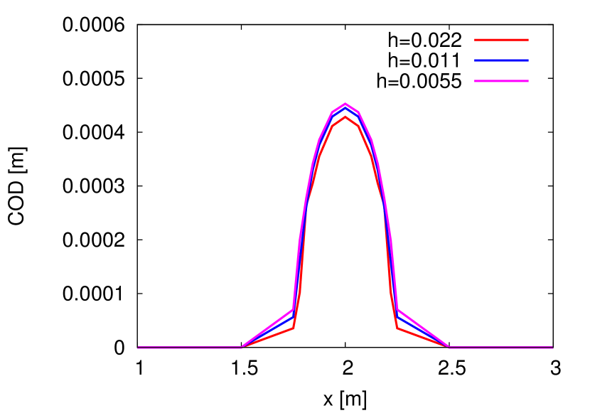
(a) $\alpha=0$

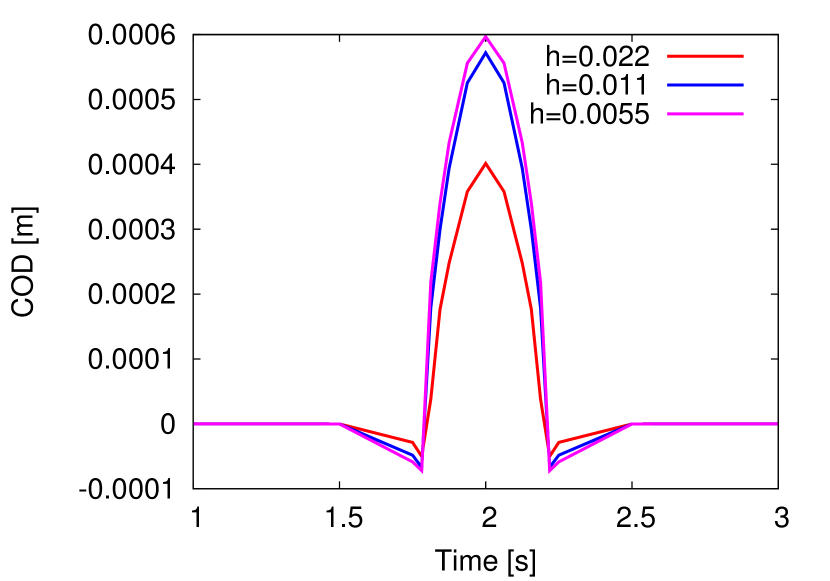
(b) $\alpha=1$

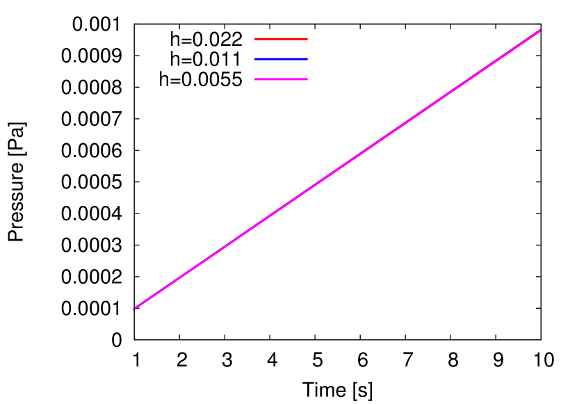
(c) $\alpha=0$

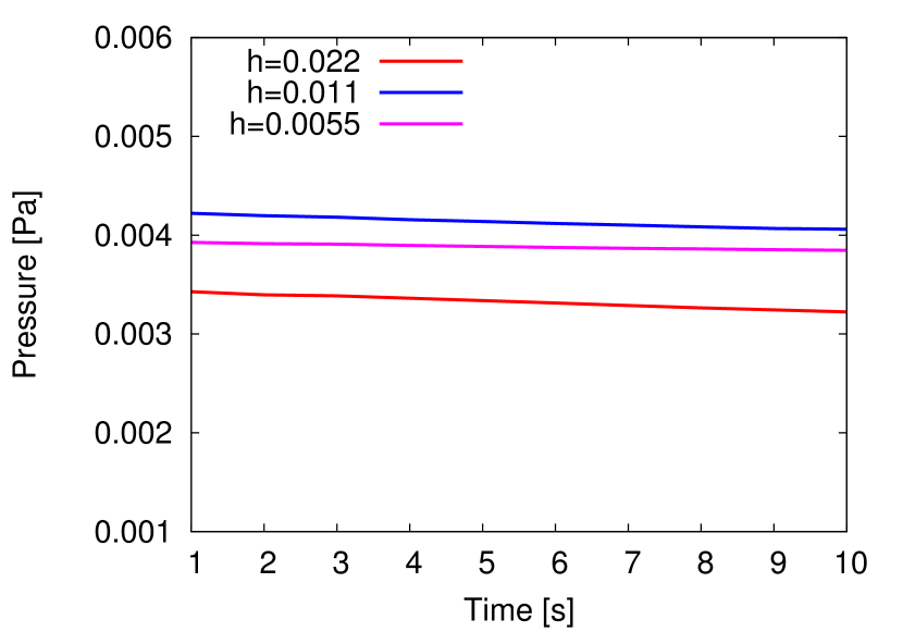
(d) $\alpha=1$

Figure 6: Example 1: On top: the crack opening displacement for (a) $\alpha=0$ and (b) $\alpha=1$ at $T=10s$. On the bottom: (c) - (d) the corresponding maximal pressure evolutions. In the bottom left subfigure at $T=10s$ the desired pressure $p\approx 0.001Pa$ is reached. This test ($\alpha=0$) compares (as expected) very much to the original Sneddon’s test with a given, fixed pressure. The test with $\alpha=1$ differs since now poroelastic effects play a role that were not accounted for in Sneddon’s original derivation.

(a) phase-field $\varphi$

(b) pressure $p$

(c) ${\bf u}_{y}$ displacement

(d) interpolated width $w$

Figure 7: Example 1: Case $\alpha=0$: The phase-field $\varphi$, the pressure $p$, the ${\bf u}_{y}$ displacement, and the interpolated width $w$ are presented.

(a) phase-field $\varphi$

(b) pressure $p$

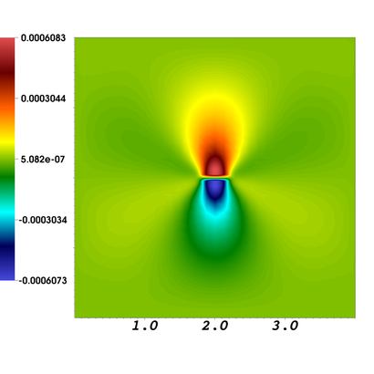
(c) ${\bf u}_{y}$ displacement

(d) interpolated width $w$

Figure 8: Example 1: Case $\alpha=1$: The phase-field $\varphi$, the pressure $p$, the ${\bf u}_{y}$ displacement, and the interpolated width $w$ are presented.

In Figure 6, we observe mesh convergence of the crack opening displacement and the corresponding pressure evolutions for both cases $\alpha=0$ and $\alpha=1$. We see that using $\alpha=0$ the pressure is $p\approx$1\text{\times}{10}^{-3}\text{\,}\mathrm{P}\mathrm{a}$$ as used by [9, 59] and yields a similar crack opening displacement. This is a major achievement that the fluid-filled model (namely pressure diffraction coupled to displacement/phase-field) is able to represent the manufactured solution of the original pressurized test case. Using $\alpha=1$ we observe that the pressures are $4$ times higher (yielding a slightly higher COD). This is expected since in the $\alpha=1$-case the fracture pressure interacts with the reservoir pressure and fluid is released into the porous medium. In the Figures 7 and 8 the different solution variables at the end time value $T=10s$ are displayed. In fact we nicely identify the interpolated width $w$ and also the different pressure distributions depending on the different $\alpha$ choices. Moreover, observing the quantitative values for ${\bf u}_{y}$ (which corresponds in this symmetric test to the COD) and the subsequent FE width value, we identify excellent agreement.

6.2 Example 2: A fluid-filled fracture with emphasis on the pressure at the fracture tips.

In this short section, we only focus on the pressure evolution for a fluid-filled (namely choosing $\alpha=1$) configuration. We highlight negative pressure values at the fracture tips, which are known as a typical phenomena caused by fluid lagging in the early injection stages and has been observed by others as well, see for example [15, 33, 49, 50, 51].

Configuration

In the domain $\Omega=(-$5\text{\,}\mathrm{m}$,$5\text{\,}\mathrm{m}$)^{2}$ the initial penny shaped fracture is given in the center $(0,0)$ with the longer radius $r=$1\text{\,}\mathrm{m}$$ on $\Omega_{F}=(4,6)\times(5-h_{\max},5+h_{\max})\subset\Omega$. The physical parameters are chosen as $\alpha=1$, $E=$1\text{\,}\mathrm{Pa}$,\nu=0.2$, $G_{c}=$1.0\text{\,}\mathrm{N}\text{\,}{\mathrm{m}}^{-1}$$, $\eta_{R}=\eta_{F}=$1\text{\times}{10}^{-3}\text{\,}\mathrm{N}\mathrm{s}\mathrm{/}\mathrm{m}^{2}$$, $\rho=$1\text{\,}\mathrm{k}\mathrm{g}\mathrm{/}\mathrm{m}^{3}$$, $K_{R}=$1\text{\times}{10}^{-16}\text{\,}\mathrm{m}^{2}$$ and $q_{F}=$7.5\text{\times}{10}^{-2}\text{\,}\mathrm{m}^{3}\mathrm{/}\mathrm{s}$$. Here the numerical parameters are given as $h_{\min}=$0.028\text{\,}\mathrm{m}$$, $\delta t=$0.5\text{\,}\mathrm{s}$$, $T=$30\text{\,}\mathrm{s}$$, and $\varepsilon=2h_{\min}$.

Discussion of our findings

At the early stage of the fluid injection, Figure 9 illustrates the pressure values in the fracture. We notice that our findings show a qualitative similarity with the plots presented in [49, 27]. However, due to $\alpha=1$, the full coupling of a fluid-filled fracture with the surrounding porous medium, and the use of another well model, we cannot expect a quantitative agreement with [49, 27]. However, the important result is that (as predicted in the above mentioned papers) that we observe negative pressures around the fracture tips. This phenomena may arise in the case of injections if the speed at which the crack tip advances is sufficiently high such that the fluid inside the fracture cannot flow fast enough to fill the created space. In particular, at the beginning of an injection, the fracture is not yet completely filled with fluid and thus at the tips fluid enters from the porous medium into the fracture causing the predicted negative pressure values.

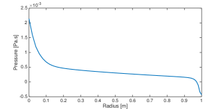
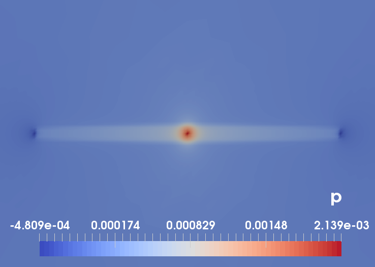
Figure 9: Example 2. Illustration of the pressure values a) inside (plotted from the center to the end-tip) and b) around the fracture. We observe negative pressures at the fracture tip.

6.3 Example 3: A propagating fluid-filled fracture in a porous medium

In this third example, we consider a single propagating fracture. The main purpose is to study fixed-stress iterations for this nonstationary case.

Configuration

We deal with the following geometric data: $\Omega=($0\text{\,}\mathrm{m}$,$4\text{\,}\mathrm{m}$)^{2}$ and a (prescribed) initial crack with half length $l_{0}=$0.2\text{\,}\mathrm{m}$$ on $\Omega_{F}=(1.8,2.2)\times(2-h_{\max},2+h_{\max})\subset\Omega$. The initial mesh is $5$ times uniformly refined, and then $2,3,4$ and $5$ times locally using predictor-corrector mesh refinement, sufficiently large around the fracture region. The number of mesh cells will grow during the computation due to predictor-corrector mesh refinement.

Parameters

The fracture toughness is chosen as $G_{c}=$1\text{\,}\mathrm{N}\text{\,}{\mathrm{m}}^{-1}$$. The mechanical parameters are Young’s modulus and Poisson’s ratio $E=${10}^{8}\text{\,}\mathrm{Pa}$$ and $\nu_{s}=0.2$. The regularization parameters are chosen as $\varepsilon=2h$ and $\kappa=${10}^{-10}$h$. We perform computations for Biot’s coefficient $\alpha=1$ only. Furthermore the injection rate is chosen as $q_{F}=$2\text{\,}\mathrm{m}^{3}\mathrm{/}\mathrm{s}$$; and $M=$1\text{\times}{10}^{8}\text{\,}\mathrm{P}\mathrm{a}$,c_{F}=$1\text{\times}{10}^{-8}\text{\,}\mathrm{P}\mathrm{a}^{-1}$$. The viscosities are chosen as $\nu_{R}=\nu_{F}=$1\text{\times}{10}^{-3}\text{\,}\mathrm{N}\mathrm{s}\mathrm{/}\mathrm{m}^{2}$$. The reservoir permeability is $K_{R}=$1\text{\,}\mathrm{d}$$ and the density is $\rho_{F}^{0}=$1\text{\,}\mathrm{k}\mathrm{g}\mathrm{/}\mathrm{m}^{3}$$. Furthermore, $TOL_{FS}=10^{-3}$. The total time is $T=$0.6\text{\,}\mathrm{s}$$. We also perform time convergence studies and use as time steps $\delta t=0.01s,0.005s,0.0025s,0.00125s$. Thus, $60,120,240$ and $480$ time steps are computed, respectively.

Quantities of interest

We study the following cases and goal functionals:

• the number of GMRES iterations within the Newton solver.

• the number of fixed-stress iterations and Newton solves for the displacement/phase-field system (Figure 14);

• the maximum pressure and the crack length/pattern evolution over time (Figure 11);

Discussion of findings

The average number of Newton iterations for the displacement/phase-field system is $4-8$ iterations per mesh per time step. The average number of GMRES iterations is $10-50$ but can go up in certain steps (just before the Newton tolerance is satisfied) up to $100-150$, which is still acceptable. To study fixed-stress iterations, computations are performed on different mesh levels in order to see the dependence of the number of mesh cells. Moreover, the presentation is divided into the number of fixed-stress iterations per mesh per time step and secondly, into the accumulated number (summing up all predictor-corrector mesh refinements) per time step, see Figure 14. In Figure 11, we study temporal convergence of two quantities of interest; namely, the pressure and the fracture length. Here we identify convergence although it is slow. With regard to the complexity of the overall problem, it is however a major accomplishment to obtain in the first place temporal convergence. This is an important finding with regard to the computational stability of the proposed framework. We remark that almost identical computational results were observed by using either Formulation 3 or Formulation 4. However, Formulation 3 is more expensive since an additional scalar-valued problem has to be solved. Finally, in Figure 12, the pressure, the crack length in terms of the phase-field variable, and the locally refined mesh are visualized.

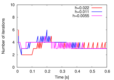
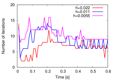
Figure 10: Example 3: Number of fixed-stress iterations per mesh per time step (at left). At right, the accumulated number of all predictor-corrector mesh levels per time step is displayed. The time step size in this test case $\delta t=0.01s$.

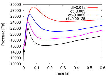
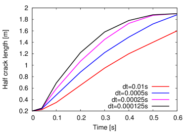
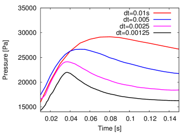
Figure 11: Example 3: Maximal pressure evolution and half crack length evolution on the finest mesh level. The time step sizes $\delta t$ are refined in order to study convergence in time. The maximal (theoretical) half length would be $2m$ (the boundary of the domain), and the fractures stop growing towards $1.9m$. Spatial refinement is not considered since both $\varepsilon$ and $h$ are varied via $\varepsilon=2h$ and convergence to common values cannot be expected. In the bottom row, zoom-ins are provided showing more clearly temporal convergence although it is very slow.

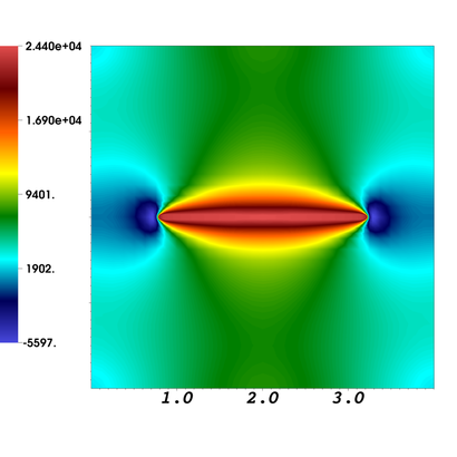
Figure 12: Example 3: Pressure evolution including negative pressure at the fracture tips (top), crack propagation (middle), and adaptive mesh evolution (bottom) at $T=0.01,0.1,0.4,0.6s$ and on the finest mesh level Ref. 5.

6.4 Example 4: Fracture networks in homogeneous and heterogeneous porous media

In this example, we study the fixed-stress algorithm for multiple fractures in homogeneous and heterogeneous porous media. In total, we have three test cases: homogeneous, a heterogeneous example in which the Lamé parameters are varied, and a third example in which additionally the reservoir permeability is non-homogeneous.

Configuration

We deal with the following geometric data: $\Omega=($0\text{\,}\mathrm{m}$,$10\text{\,}\mathrm{m}$)^{2}$ and three initial cracks.

Parameters

The fracture toughness is chosen as $G_{c}=$1\text{\,}\mathrm{N}\text{\,}{\mathrm{m}}^{-1}$$. The mechanical parameters are Young’s modulus and Poisson’s ratio $E=${10}^{8}\text{\,}\mathrm{Pa}$$ and $\nu_{s}=0.2$ for the homogeneous case. In the heterogeneous setting, we have $${10}^{7}\text{\,}\mathrm{Pa}$\leq E\leq${10}^{8}\text{\,}\mathrm{Pa}$$. These heterogeneities are chosen as such that the length-scale parameter $\varepsilon$ can resolve them; see Figure 13.

Figure 13: Example 4: Heterogeneous solid. Display of $\mu$. These data are synthetic using a random distribution. In particular, the heterogeneities are chosen as such that $\varepsilon$ can resolve them, i.e., $l>\varepsilon=2h$, where $l$ is the length-scale of the material inhomogeneity (at right).

The regularization parameters are chosen as $\varepsilon=2h$ and $\kappa=${10}^{-10}$h$. Biot’s coefficient is $\alpha=1$. Furthermore $q_{F}=$5\text{\,}\mathrm{m}^{3}\mathrm{/}\mathrm{s}$$ and $M=$1\text{\times}{10}^{8}\text{\,}\mathrm{P}\mathrm{a}$,c_{F}=$1\text{\times}{10}^{-8}\text{\,}\mathrm{P}\mathrm{a}$$. The viscosities are chosen as $\nu_{R}=\nu_{F}=$1\text{\times}{10}^{-3}\text{\,}\mathrm{N}\mathrm{s}\mathrm{/}\mathrm{m}^{2}$$. The reservoir permeability is $K_{R}=$1\text{\,}\mathrm{d}$$ in the homogeneous case and varies $0.1d\leq K_{R}\leq 1d$ in the heterogeneous setting. and the density is $\rho_{F}^{0}=$1\text{\,}\mathrm{k}\mathrm{g}\mathrm{/}\mathrm{m}^{3}$$. The time step size is $\delta t=$1\text{\times}{10}^{-2}\text{\,}\mathrm{s}$$ and the final time is not specified and rather taken when all fractures joined. This event takes place between $0.25s\leq T\leq 0.3s$. Furthermore, $TOL_{FS}=10^{-4}$ (for the pressure and the displacements), whereas the phase-field tolerance is chosen as $TOL_{FS}=10^{-2}$. In fact the convergence of the phase-field variable is much harder for multiple fractures and heterogeneous media than in the previous examples.

Quantities of interest

In this example, we observe the crack pattern, the pressure distribution, and fixed-stress iterations.

Discussion of findings

In Figure 14, the number of fixed-stress iterations per time step is shown. The evolution of the pressure and the fracture patterns at different times are displayed in Figure 15 and Figure 16. The average number of non-linear iterations of the semi-smooth Newton solver for the three test cases are $8-10$, with in average $10-20$ linear GMRES iterations. Here, we do not observe a significant difference between homogeneous and heterogeneous media. Furthermore, we observe again the same crack pattern for both level-set formulations, but using Formulation 4 the final shape is reached earlier. Due to the complexity of this test (multiple fractures and heterogeneous materials) further future investigations are definitely necessary.

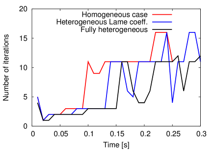
Figure 14: Example 4: The number of fixed-stress iterations per time step. The time step size in this test case $\delta t=0.01s$.

Figure 15: Example 4: Homogeneous test case. Display of pressure (top) and fracture pattern at $T=0s,0.1s,0.2s,0.25s$.

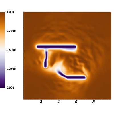
Figure 16: Example 4: Heterogeneous test case with varying Lamé parameters and homogeneous reservoir permeability. Display of pressure (top) and fracture pattern at $T=0s,0.1s,0.2s,0.3s$.

Figure 17: Example 4: Fully heterogeneous test case. Display of pressure (top) and fracture pattern at $T=0s,0.1s,0.2s,0.3s$.

6.5 Example 5: Propagating penny-shaped fracture in 3D

In this final example, we consider a penny shaped fracture in a three dimensional domain $\Omega=(0,$4\text{\,}\mathrm{m}$)^{3}$. The horizontal initial penny shape crack is centered at $($2\text{\,}\mathrm{m}$,$2\text{\,}\mathrm{m}$,$2\text{\,}\mathrm{m}$)$ on $y=$2\text{\,}\mathrm{m}$-$ plane and we refine around the crack; see Figure 18(a) for the setup. Initial and boundary conditions are same as previous examples and here the physical parameters are given. The fracture toughness is chosen as $G_{c}=$1\text{\,}\mathrm{N}\text{\,}{\mathrm{m}}^{-1}$$, Young’s modulus and Poisson’s ratio as $E=${10}^{8}\text{\,}\mathrm{Pa}$$ and $\nu_{s}=0.2$, respectively. The regularization parameters are chosen as $\varepsilon=2h_{\min}$ and $\kappa=${10}^{-10}$h$. The Biot coefficient and Biot’s modulus are set to $\alpha=1$ and $M=$1\text{\times}{10}^{8}\text{\,}\mathrm{P}\mathrm{a}$$, respectively. Furthermore we assume a slightly incompressible fluid with $c_{F}=$1\text{\times}{10}^{-8}\text{\,}\mathrm{P}\mathrm{a}$$ and the viscosities are chosen as $\eta_{R}=\eta_{F}=$1\text{\times}{10}^{-3}\text{\,}\mathrm{N}\mathrm{s}\mathrm{/}\mathrm{m}^{2}$$ with the injection rate $q_{F}=$2\text{\,}\mathrm{m}^{3}\mathrm{/}\mathrm{s}$$. The reservoir permeability is $K_{R}=$1\text{\,}\mathrm{d}$$ and the density is $\rho_{F}^{0}=$1\text{\,}\mathrm{k}\mathrm{g}\mathrm{/}\mathrm{m}^{3}$$. Furthermore, $h_{\min}=$0.05\text{\,}\mathrm{m}$$, $\delta t=$1\text{\times}{10}^{-2}\text{\,}\mathrm{s}$$, and $TOL_{FS}=10^{-3}$.

Figure 18(b)-18(d) illustrate the propagating fracture for each time. The crack opening displacement and the fixed stress iteration number over the time for propagating fracture are shown in Figure 19. We note that the almost identical computational results were observed by employing either Formulation 3 or Formulation 4 to compute the level-set as shown in previous example. However, Formulation 4 is computationally more efficient especially in three dimensional cases.

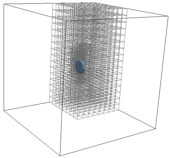
(a) Setup

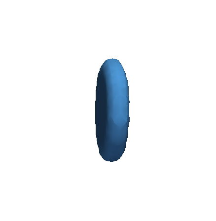
(b) $n=30$

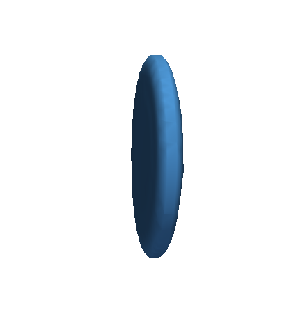
(c) $n=50$

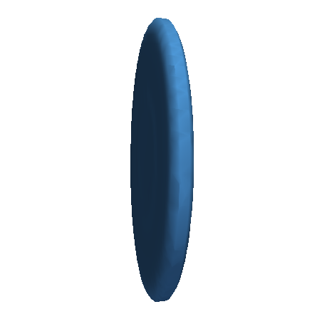
(d) $n=100$

Figure 18: Example 6.5: (a) The initial penny shape crack is centered at $($5\text{\,}\mathrm{m}$,$5\text{\,}\mathrm{m}$,$5\text{\,}\mathrm{m}$)$ on $y=$5\text{\,}\mathrm{m}$-$plane with the mesh refinement. (b)-(d) illustrate the propagating fracture for each time step.

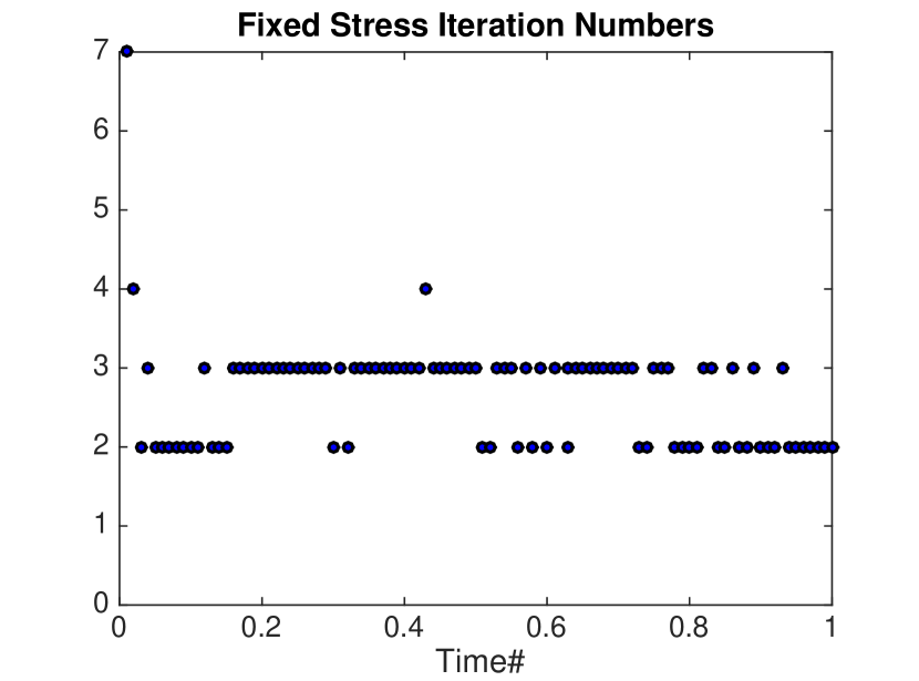
(a) Fixed stress iteration number

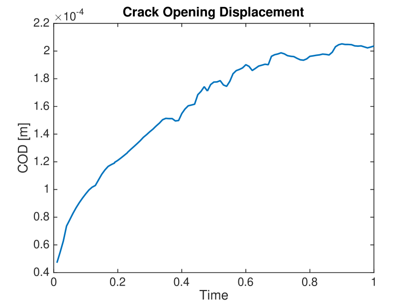
(b) Crack opening displacement $\|w\|_{L^{\infty}(\Lambda)}$.

Figure 19: (a) Fixed stress iteration number over the time with a three dimensional MPI computation is shown. (b) crack width opening over the time for the propagating fracture.

7 Conclusions

In this paper, we presented fixed-stress splitting for fractured porous media using a phase-field technique. Several examples were consulted in order to show the performance of the algorithmic techniques. Despite the complexity of the entire problem, we could observe spatial and temporal convergence of selected quantities of interest. This is a major step towards the computational stability and reliability of our proposed method. Moreover, we could observe typical properties of fluid-filled fractures, namely a negative pressure at the fracture tips, which are not present when Biot’s coefficient is zero. Moreover, we investigated the solver iteration numbers for the linear iterative GMRES solver, the nonlinear Newton solver of the displacement/phase-field system, and the fixed stress iterations between flow and mechanics. For our settings, we obtained efficient iterations numbers as shown in our numerical examples. However, in Example 4, heterogeneous materials, we observed that the convergence is dominated by the phase-field variable whereas the pressure and the displacements converges well. We finally mention that the level-set width computation shows a novel way to obtain accurate width values inside the fracture region. This holds in particular true for homogeneous test cases (Examples 1-3 and Example 5). For heterogeneous tests and multiple fractures (Example 4), we also obtained good results but it is still an open question whether the methodology works for arbitrary heterogeneous materials which goes beyond the current paper and is left for future research.

References

- [1] L. Ambrosio and V. Tortorelli. Approximation of functionals depending on jumps by elliptic functionals via -convergence. Comm. Pure Appl. Math., 43:999–1036, 1990.
- [2] L. Ambrosio and V. Tortorelli. On the approximation of free discontinuity problems. Boll. Un. Mat. Ital. B, 6:105–123, 1992.
- [3] H. Amor, J.-J. Marigo, and C. Maurini. Regularized formulation of the variational brittle fracture with unilateral contact: Numerical experiments. Journal of Mechanics Physics of Solids, 57:1209–1229, Aug. 2009.
- [4] W. Bangerth, D. Davydov, T. Heister, L. Heltai, G. Kanschat, M. Kronbichler, M. Maier, B. Turcksin, and D. Wells. The deal.II library, version 8.4. Journal of Numerical Mathematics, 24, 2016.
- [5] W. Bangerth, R. Hartmann, and G. Kanschat. deal.II – a general purpose object oriented finite element library. ACM Trans. Math. Softw., 33(4):24/1–24/27, 2007.
- [6] A. Bonito, J.-L. Guermond, and S. Lee. Numerical simulations of bouncing jets. International Journal for Numerical Methods in Fluids, 80(1):53–75, 2016.
- [7] M. J. Borden, C. V. Verhoosel, M. A. Scott, T. J. R. Hughes, and C. M. Landis. A phase-field description of dynamic brittle fracture. Comput. Meth. Appl. Mech. Engrg., 217:77–95, 2012.
- [8] B. Bourdin. Numerical implementation of the variational formulation for quasi-static brittle fracture. Interfaces and free boundaries, 9:411–430, 2007.
- [9] B. Bourdin, C. Chukwudozie, and K. Yoshioka. A variational approach to the numerical simulation of hydraulic fracturing. SPE Journal, Conference Paper 159154-MS, 2012.
- [10] B. Bourdin, G. Francfort, and J.-J. Marigo. Numerical experiments in revisited brittle fracture. J. Mech. Phys. Solids, 48(4):797–826, 2000.
- [11] B. Bourdin, G. Francfort, and J.-J. Marigo. The variational approach to fracture. J. Elasticity, 91(1–3):1–148, 2008.
- [12] B. Bourdin, J.-J. Marigo, C. Maurini, and P. Sicsic. Morphogenesis and propagation of complex cracks induced by thermal shocks. Phys. Rev. Lett., 112:014301, Jan 2014.
- [13] S. Burke, C. Ortner, and E. Süli. An adaptive finite element approximation of a variational model of brittle fracture. SIAM J. Numer. Anal., 48(3):980–1012, 2010.
- [14] N. Castelletto, J. A. White, and H. A. Tchelepi. Accuracy and convergence properties of the fixed-stress iterative solution of two-way coupled poromechanics. International Journal for Numerical and Analytical Methods in Geomechanics, 39(14):1593–1618, 2015.
- [15] E.Detournay and D. Garagash. The near-tip region of a fluid-driven fracture propagating in a permeable elastic solid. J. Fluid Mech., 494:1–32, 2003.
- [16] G. Francfort and J.-J. Marigo. Revisiting brittle fracture as an energy minimization problem. J. Mech. Phys. Solids, 46(8):1319–1342, 1998.
- [17] T. Gerasimov and L. D. Lorenzis. A line search assisted monolithic approach for phase-field computing of brittle fracture. Computer Methods in Applied Mechanics and Engineering, pages –, 2015.
- [18] V. Girault, K. Kumar, and M. F. Wheeler. Convergence of iterative coupling of geomechanics with flow in a fractured poroelastic medium. Computational Geosciences, pages 1–15, 2016.
- [19] Y. Heider and B. Markert. A phase-field modeling approach of hydraulic fracture in saturated porous media. Mechanics Research Communications, pages –, 2016.
- [20] T. Heister, M. F. Wheeler, and T. Wick. A primal-dual active set method and predictor-corrector mesh adaptivity for computing fracture propagation using a phase-field approach. Comput. Methods Appl. Mech. Engrg., 290:466–495, 2015.
- [21] M. Heroux, R. Bartlett, V. H. R. Hoekstra, J. Hu, T. Kolda, R. Lehoucq, K. Long, R. Pawlowski, E. Phipps, A. Salinger, H. Thornquist, R. Tuminaro, J. Willenbring, and A. Williams. An Overview of Trilinos. Technical Report SAND2003-2927, Sandia National Laboratories, 2003.
- [22] S.-R. Hysing. Numerical simulation of immiscible fluids with FEM level set techniques. PhD thesis, Technical University of Dortmund, 2008.
- [23] J. Kim, H. Tchelepi, and R. Juanes. Stability, accuracy, and efficiency of sequentiel methods for flow and geomechanics. SPE Journal, 16(2):249–262, 2011.
- [24] J. Kim, H. Tchelepi, and R. Juanes. Stability and convergence of sequentiel methods for coupled flow and geomechanics: fixed-stress and fixed-strain splits. Comp. Methods Appl. Mech. Engrg., 200(13-16):1591–1606, 2011.
- [25] Y. Kovalyshen. Fluid-driven fracture in poroelastic medium. PhD thesis, The University of Minnesota, 2010.
- [26] O. Ladyzhenskaja, V. Solonnikov, and N. Uralceva. Linear and quasi-linear equations of parabolic type. Translations of mathematical monographs, AMS Vol. 23, 1968.
- [27] B. Lecampion, A. Peirce, E. Detournay, X. Zhang, Z. Chen, A. Bunger, C. Detournay, J. Napier, S. Abbas, D. Garagash, and P. Cundall. The Impact of the Near-Tip Logic on the Accuracy and Convergence Rate of Hydraulic Fracture Simulators Compared to Reference Solutions. In Effective and Sustainable Hydraulic Fracturing. InTech, May 2013.
- [28] S. Lee, Y.-J. Lee, and M. F. Wheeler. A locally conservative enriched galerkin approximation and efficient solver for elliptic and parabolic problems. SIAM Journal on Scientific Computing, 38(3):A1404–A1429, 2016.
- [29] S. Lee, A. Mikelić, M. F. Wheeler, and T. Wick. Phase-field modeling of proppant-filled fractures in a poroelastic medium. Comput. Meth. Appl. Mech. Engrg., 2016.
- [30] S. Lee, J. E. Reber, N. W. Hayman, and M. F. Wheeler. Investigation of wing crack formation with a combined phase-field and experimental approach. Geophysical Research Letters, 43(15):7946–7952, 2016.
- [31] S. Lee, M. F. Wheeler, and T. Wick. Pressure and fluid-driven fracture propagation in porous media using an adaptive finite element phase field model. Computer Methods in Applied Mechanics and Engineering, 305:111 – 132, 2016.
- [32] S. Lee, M. F. Wheeler, T. Wick, and S. Srinivasan. Initialization of phase-field fracture propagation in porous media using probability maps of fracture networks. Mechanics Research Communications, 2016.
- [33] B. Markert and Y. Heider. Recent Trends in Computational Engineering - CE2014: Optimization, Uncertainty, Parallel Algorithms, Coupled and Complex Problems, chapter Coupled Multi-Field Continuum Methods for Porous Media Fracture, pages 167–180. Springer International Publishing, Cham, 2015.
- [34] A. Mesgarnejad, B. Bourdin, and M. Khonsari. Validation simulations for the variational approach to fracture. Computer Methods in Applied Mechanics and Engineering, 290:420 – 437, 2015.
- [35] C. Miehe, M. Hofacker, L.-M. Schaenzel, and F. Aldakheel. Phase field modeling of fracture in multi-physics problems. part ii. coupled brittle-to-ductile failure criteria and crack propagation in thermo-elastic–plastic solids. Computer Methods in Applied Mechanics and Engineering, 294:486 – 522, 2015.
- [36] C. Miehe, M. Hofacker, and F. Welschinger. A phase field model for rate-independent crack propagation: Robust algorithmic implementation based on operator splits. Comput. Meth. Appl. Mech. Engrg., 199:2765–2778, 2010.
- [37] C. Miehe and S. Mauthe. Phase field modeling of fracture in multi-physics problems. part iii. crack driving forces in hydro-poro-elasticity and hydraulic fracturing of fluid-saturated porous media. Computer Methods in Applied Mechanics and Engineering, pages –, 2015.
- [38] C. Miehe, S. Mauthe, and S. Teichtmeister. Minimization principles for the coupled problem of darcy–biot-type fluid transport in porous media linked to phase field modeling of fracture. Journal of the Mechanics and Physics of Solids, 82:186 – 217, 2015.
- [39] C. Miehe, L.-M. Schaenzel, and H. Ulmer. Phase field modeling of fracture in multi-physics problems. part i. balance of crack surface and failure criteria for brittle crack propagation in thermo-elastic solids. Computer Methods in Applied Mechanics and Engineering, 294:449 – 485, 2015.
- [40] C. Miehe, F. Welschinger, and M. Hofacker. Thermodynamically consistent phase-field models of fracture: variational principles and multi-field fe implementations. International Journal of Numerical Methods in Engineering, 83:1273–1311, 2010.
- [41] A. Mikelić, B. Wang, and M. F. Wheeler. Numerical convergence study of iterative coupling for coupled flow and geomechanics. Computational Geosciences, 18(3-4):325–341, 2014.
- [42] A. Mikelić and M. F. Wheeler. Convergence of iterative coupling for coupled flow and geomechanics. Comput Geosci, 17(3):455–462, 2012.
- [43] A. Mikelić, M. F. Wheeler, and T. Wick. A phase-field method for propagating fluid-filled fractures coupled to a surrounding porous medium. SIAM Multiscale Model. Simul., 13(1):367–398, 2015.
- [44] A. Mikelić, M. F. Wheeler, and T. Wick. Phase-field modeling of a fluid-driven fracture in a poroelastic medium. Computational Geosciences, 19(6):1171–1195, 2015.
- [45] A. Mikelić, M. F. Wheeler, and T. Wick. A quasi-static phase-field approach to pressurized fractures. Nonlinearity, 28(5):1371–1399, 2015.
- [46] T. Nguyen, J. Yvonnet, Q.-Z. Zhu, M. Bornert, and C. Chateau. A phase-field method for computational modeling of interfacial damage interacting with crack propagation in realistic microstructures obtained by microtomography. Computer Methods in Applied Mechanics and Engineering, pages –, 2015.
- [47] D. A. D. Pietro and A. Ern. Mathematical Aspects of Discontinuous Galerkin Methods, volume 69 of Mathematiques et Applications. Society for Industrial and Applied Mathematics (SIAM), Berlin-Heidelberg, 2012.
- [48] B. Riviere. Discontinuous Galerkin Methods for Solving Elliptic and Parabolic Equations: Theory and Implementation. SIAM, 2008.
- [49] A. Savitski and E. Detournay. Propagation of a penny-shaped fluid-driven fracture in an impermeable rock: asymptotic solutions. International Journal of Solids and Structures, 39:6311–6337, 2002.
- [50] B. A. Schrefler, S. Secchi, and L. Simoni. On adaptive refinement techniques in multi-field problems including cohesive fracture. Comput. Meth. Appl. Mech. Engrg., 195:444–461, 2006.
- [51] S. Secchi and B. A. Schrefler. A method for 3-d hydraulic fracturing simulation. Int. J. Fract., 178:245–258, 2012.
- [52] A. Settari and F. Mourits. A coupled reservoir and geomechanical simulation system. SPE Journal, 3(3):219–226, 1998.
- [53] A. Settari and D. A. Walters. Advances in coupled geomechanical and reservoir modeling with applications to reservoir compaction. SPE Journal, 6(3):334–342, Sept. 2001.
- [54] G. Singh, G. Pencheva, K. Kumar, T. Wick, B. Ganis, and M. F. Wheeler. Impact of accurate fractured reservoir flow modeling on recovery predictions. SPE 188630-MS, SPE Hydraulic Fracturing Technology Conference, Woodlands, TX, 2014.
- [55] I. N. Sneddon. The distribution of stress in the neighbourhood of a crack in an elastic solid. Proc. R Soc London A, 187:229–260, 1946.
- [56] I. N. Sneddon and M. Lowengrub. Crack problems in the classical theory of elasticity. SIAM series in Applied Mathematics. John Wiley and Sons, Philadelphia, 1969.
- [57] C. V. Verhoosel and R. de Borst. A phase-field model for cohesive fracture. Int. J. Numer. Meth. Engrg., 96:43–62, 2013.
- [58] J. Vignollet, S. May, R. Borst, and C. V. Verhoosel. Phase-field models for brittle and cohesive fracture. Meccanica, 49(11):2587–2601, 2014.
- [59] M. F. Wheeler, T. Wick, and W. Wollner. An augmented-Lagangrian method for the phase-field approach for pressurized fractures. Comp. Meth. Appl. Mech. Engrg., 271:69–85, 2014.
- [60] T. Wick. Goal functional evaluations for phase-field fracture using PU-based DWR mesh adaptivity. Computational Mechanics, pages 1–19, 2016.
- [61] T. Wick, S. Lee, and M. F. Wheeler. 3D phase-field for pressurized fracture propagation in heterogeneous media. VI International Conference on Computational Methods for Coupled Problems in Science and Engineering 2015 Proceedings, May 2015.
- [62] T. Wick, G. Singh, and M. Wheeler. Fluid-filled fracture propagation using a phase-field approach and coupling to a reservoir simulator. SPE Journal, pages 1–19, 2015.
- [63] Z. A. Wilson and C. M. Landis. Phase-field modeling of hydraulic fracture. Journal of the Mechanics and Physics of Solids, 96:264 – 290, 2016.