Deuteron properties from muonic atom spectroscopy

Abstract

Leading order ($\alpha^{4}$) finite size corrections in muonic deuterium are evaluated within a few body formalism for the $\mu^{-}pn$ system in muonic deuterium and found to be sensitive to the input of the deuteron wave function. We show that this sensitivity, taken along with the precise deuteron charge radius determined from muonic atom spectroscopy can be used to determine the elusive deuteron D-state probability, $P_{D}$, for a given model of the nucleon-nucleon (NN) potential. The radius calculated with a $P_{D}$ of 4.3% in the chiral NN models and about 5.7% in the high precision NN potentials is favoured most by the $\mu^{-}d$ data.

I Introduction

The lightest nucleus, namely, the deuteron, has traditionally held an important place in nuclear physics as a testing ground for the nucleon-nucleon interaction. Determining the D-state probability in the deuteron wave function in particular has been a classic problem of nuclear physics feshschwin ; rodningsboth ; oller . Stating the problem in simple words, the deuteron has a quadrupole moment and hence cannot be in a pure S-state but rather a D-state admixture is required. However, as it was shown in amadofriar that the D-state probability, $P_{D}=\int_{0}^{\infty}w^{2}(r)dr$ (with $w(r)$ being the deuteron radial wave function with $l=2$), is inaccessible directly to experiments, it is usually the asymptotic D-state to S-state wave function ratio, $\eta$ rodningsboth ; conzet , which is determined. There do exist attempts to determine $P_{D}$ from the measured magnetic moment of the deuteron, $\mu_{D}$, with, $\mu_{D}=\mu_{S}-(3/2)P_{D}(\mu_{S}-1/2)+\delta_{R}$, where, $\mu_{S}=\mu_{P}+\mu_{N}$ is the isoscalar nucleon magnetic moment. However, the term $\delta_{R}$ which includes mesonic exchange effects, relativistic corrections, dynamical effects and isobar configurations in the deuteron introduces uncertainties in the extraction of $P_{D}$ michael . This fact was noticed in one of the oldest works by Feshbach and Schwinger feshschwin on the theory of nuclear forces which gave the D-state probability, $P_{D}$, ranging between 2% to 6%. Much later, Ref. mathel listed values of $P_{D}$ ranging from 0.28 to 6.47% for 9 different nucleon-nucleon (NN) potentials. However, earlier in levin the possible minimum was shown to be 0.45%. With $P_{D}$ not being a measurable quantity, Refs rodningsboth and conzet determined the asymptotic ratio $\eta$ = 0.0256 $\pm$ 0.0004 and 0.0268 $\pm$ 0.0013 from tensor analyzing powers in sub-Coulomb ($d,p$) reactions and $dp$ elastic scattering respectively. In the absence of a “measured” D-state probability, theoretical models of the NN interaction also try to reproduce the asymptotic ratio $\eta$ determined from experiments (in addition to other data) to confirm the reliability of the NN model oller .

The purpose of this work is to present a new method which provides a means to fix the percentage of the “elusive” amadofriar D-state probability, $P_{D}$, from experiments in an indirect manner. The method is particularly useful in view of the very high precision reported by recent muonic deuterium experiments pohldeut . It is based on a few body calculation of the leading order ($\alpha^{4}$) finite size corrections (FSC) to the energy levels of muonic deuterium atoms. There exists extensive literature on corrections including the deuteron polarization leidman ; pachucki ; bacca , with detailed calculations of FSC at higher orders ($\alpha^{5}$, $\alpha^{6}$ etc) friarseminal ; leidman ; pachucki ; bacca . The sensitivity of the higher order FSC to the form of the nucleon-nucleon potential (and hence the deuteron wave function) is found to be small leidman ; bacca or negligible friarzero . The leading FSC at order $\alpha^{4}$ in these works is written in terms of the deuteron charge radius. The few body formalism of the present work helps in revealing the dependence of the leading FSC term on the proton and neutron form factors as well as the deuteron wave function. We show that a comparsion of the order $\alpha^{4}$ FSC with those of Ref. pohldeut where the radius is precisely extracted from measurements in muonic deuterium provides a method to adjust the deuteron D-state probability. To be specific, we present calculations using different parametrizations of the deuteron wave function (with different amounts of the D-state probabilities) and compare the corrections with those given in pohldeut in a form dependent on the deuteron charge radius, $r_{d}$. Though the general trend of the results is an increase in the radius for smaller values of $P_{D}$, the results are found to depend on the type of model used. In the class of chiral models chiralNN , $P_{D}$ = 4.3% is found to be favourable for the closest agreement with the precise value of $r_{d}=2.12562(78)$ fm pohldeut . Using high precision NN potentials such as Nijmegen, Reid, Paris etc highNN , $P_{D}$ = 5.7% to 5.8% is favoured by the $\mu d$ data.

II Finite size effects in muonic deuterium

Finite size corrections (FSC) to the energy levels in the hydrogen atom has been a topic of revived interest weproton in the past few years due to the increase in the precision achieved in atomic spectroscopy measurements. These effects are manifested more strongly in muonic atoms due to the fact that the muon is about 200 times heavier than the electron and hence has a Bohr radius which is much smaller. In view of the recent precise measurement of the Lamb shift in muonic deuterium pohldeut , it seems timely to put forth the question as to what other impact (apart from the precise radius determination) does this measurement have on physics. In order to see this, we study the effects of deuteron structure on the energy levels in this atom. The present work considers the effects at leading order ($\alpha^{4}$) and we refer the reader to leidman ; pachucki ; bacca for higher order corrections.

II.1 Electromagnetic muon-deuteron potential

We investigate the finite size effects by calculating the energy correction, $\Delta E$, using first order perturbation theory involving an electromagnetic muon-deuteron potential, $V_{\mu^{-}d}$. The latter is constructed using a three body approach to the muon-proton-neutron system with the proton and neutron being bound inside the deuteron. As we will see below, the $\mu^{-}p$ and $\mu^{-}n$ interactions are obtained using the proton and neutron electromagnetic form factors and the $pn$ interaction is contained in the deuteron wave function. Such a potential can be constructed using standard techniques from scattering theory where we first write down the scattering amplitude to obtain the potential $V_{\mu^{-}d}(\bm{q})$ in momentum space and then evaluate its Fourier transform which enters the energy correction given by, $\Delta E=\int_{0}^{\infty}\Delta{V}(r)|\Psi_{nl}(\bm{r})|^{2}d^{3}r$. This procedure of obtaining potentials in coordinate space is also common in quantum field theory wejphysg ; casimir ; nuclear . Here, $\Delta{V}$ is the difference of $V_{\mu^{-}d}(r)$ and the $\mu^{-}d$ electromagnetic potential assuming the deuteron to be point-like. Details of the few body formalism used here can be found in belyaev ; myprl . We shall repeat the relevant steps briefly below.

The Hamiltonian of the quantum system consisting of a muon and a nucleus (with A nucleons) is given as belyaev , $H=H_{0}\,+\,V_{\mu^{-}A}\,+\,H_{A}$, where $H_{0}$ is the muon-nucleus kinetic energy operator (free Hamiltonian), $V_{\mu^{-}A}=\sum_{i=1}^{A}\,V_{i}$, the sum of muon-nucleon potentials, $V_{i}\equiv V_{\mu^{-}N}(|\bm{R}-\bm{r}_{i}|)$, where $\bm{R}$ and $\bm{r}_{i}$ are the coordinates of the muon and the $i^{th}$ nucleon with respect to the centre of mass of the nucleus and $H_{A}$ is the total Hamiltonian of the nucleus containing the potential term, $\sum_{i\neq j}\,V_{NN}(|\bm{r}_{i}-\bm{r}_{j}|)$. We proceed with the assumption that the nucleus remains in its ground state during the scattering process, i.e., $H_{A}\,|\Phi\rangle=\epsilon\,|\Phi\rangle$ and that the nucleons occupy fixed positions inside the nucleus. The muon - nucleus elastic scattering amplitude can be expressed as belyaev $f(\bm{k}^{\prime},\bm{k};E)=-(\mu/\pi)\,\langle\,\bm{k}^{\prime},\Phi\,|\,T(E)\,|\bm{k},\Phi\,\rangle$ in terms of the matrix elements of the operator $T$ obeying the Lippmann-Schwinger (L-S) equation, $T=V+V(E-H_{0}-H_{A})^{-1}T$. $|\bm{k},\Phi\,\rangle$ and $|\bm{k}^{\prime},\Phi\rangle$ are the initial and final asymptotic states which differ only in the direction of the relative muon nucleus momenta $\bm{k}$ and $\bm{k}^{\prime}$. Since the electromagnetic potential, $V_{\mu^{-}\,A}$, is proportional to the coupling constant $\alpha\sim 1/137$, it is reasonable to truncate the L-S equation at first order and approximate $T=V=\sum_{i}V_{i}$. Thus, $T(\bm{k}^{\prime},\bm{k})$ = $V(\bm{k}^{\prime},\bm{k})$ and denoting, $T(\bm{k}^{\prime},\bm{k})\equiv\langle\,\bm{k}^{\prime},\Phi\,|\,T(E)\,|\bm{k},\Phi\,\rangle$, we have $V(\bm{k}^{\prime},\bm{k})\,=\,\langle\,\bm{k}^{\prime},\Phi\,|\,\sum_{i=1}^{A}\,V_{i}\,|\bm{k},\Phi\,\rangle$. If the internal Jacobi coordinates are denoted by $\bm{x}_{i}$, then relating them with $\bm{r}_{i}=a_{i}\bm{x}_{1}\,+\,b_{i}\bm{x}_{2}\,+\,...\,+\,g_{i}\bm{x}_{A-1}$, we can write,

$$V(\bm{k}^{\prime},\bm{k})=\int d\bm{x}_{1}\,d\bm{x}_{2}\,...\,d\bm{x}_{A-1}\,|\Phi(\bm{x}_{1},\bm{x}_{2},\,...)|^{2}\sum_{i=1}^{A}\,V_{i}(\bm{k}^{\prime},\bm{k},\bm{r}_{i})\,,$$ (1)

where, $V_{i}(\bm{k}^{\prime},\bm{k},\bm{r}_{i})=V_{i}(\bm{k}^{\prime},\bm{k})\,\exp[i(\bm{k}-\bm{k}^{\prime})\cdot\bm{r}_{i}]$. The above discussion is valid for any nucleus with $A$ nucleons. In case of the muon-deuteron system, this reduces to

$$V(\bm{k}^{\prime},\bm{k})\,=\,\int\,d\bm{x}_{1}\,|\Phi_{d}(\bm{x}_{1})|^{2}\,[\,V_{\mu^{-}p}(\bm{k}^{\prime},\bm{k},{1\over 2}\bm{x}_{1})\,+\,V_{\mu^{-}n}(\bm{k}^{\prime},\bm{k},-{1\over 2}\bm{x}_{1})\,]\,$$ (2)

where we used, $\bm{x}_{1}=\bm{r}_{1}-\bm{r}_{2}$, $\bm{r}_{1}=(1/2)\bm{x}_{1}$ and $\bm{r}_{2}=-(1/2)\bm{x}_{1}$. We identify $1$ and $2$ with proton and neutron so that, $V_{1}=V_{\mu^{-}p}$, $V_{2}=V_{\mu^{-}n}$ and $\Phi_{d}$ is the deuteron wave function.

To evaluate (2), we need the $\mu^{-}$-nucleon electromagnetic potential, which, with the inclusion of the nucleon electromagnetic form factors $G_{E}^{N}(q^{2})$ can be written using the formalism of the Breit equation wejphysg within the one-photon-exchange interaction. Since such a potential was explicitly derived in weproton ; wejphysg by evaluating the elastic muon-nucleon amplitude expanded in powers of $1/c^{2}$, we shall not repeat the derivation here. This potential with form factors contains 23 terms wejphysg corresponding to the (i) Coulomb potential, (ii) Darwin terms, and (iii) spin dependent terms which give rise to fine and hyperfine structure. If we consider only the scalar parts of the Breit potential, they depend only on $\bm{q}^{2}$ and hence we can write, $V_{\mu^{-}N}(\bm{k},\bm{k}^{\prime})\equiv V_{\mu^{-}N}(\bm{q})$ wejphysg ; weproton , where, $\bm{q}=\bm{k}-\bm{k}^{\prime}$ is the momentum transfer carried by the exchanged photon. Denoting $Q=|\bm{q}|$, the $\mu^{-}N$ potential is given as weproton ,

$$V_{\mu^{-}N}(Q)=-4\pi\alpha{G_{E}^{N}(Q^{2})\over Q^{2}}\,\biggl{\{}1-{Q^{2}\over 8m_{N}^{2}c^{2}}-{Q^{2}\over 8m_{\mu}^{2}c^{2}}\biggr{\}}\,,$$ (3)

where $m_{N}$ and $m_{\mu}$ are the nucleon and muon masses. $G_{E}^{N}(Q^{2})$ is the nucleon electric form factor. A Fourier transform of the first term in the curly bracket leads to the $\mu^{-}N$ Coulomb potential for a finite sized nucleon. The next two terms in the curly brackets are relativistic corrections, the Darwin terms in the muon (spin 1/2) - nucleon (spin 1/2) $\mu^{-}N$ interaction Breit potential. The Darwin term ${Q^{2}/8m_{N}^{2}c^{2}}$ is conventionally not considered as a part of the nucleon form factor $G_{E}^{N}(q^{2})$ friaradv and hence is kept explicitly in the muon-nucleon potential here. Putting together (2) and (3) we obtain the muon-deuteron electromagnetic potential, $V_{\mu^{-}d}(Q)=V_{\mu^{-}p}(Q)\int\,d\bm{x}\,|\Phi_{d}(\bm{x})|^{2}\,e^{-i\bm{q}\cdot\bm{x}/2}\,+\,V_{\mu^{-}n}(Q)\int\,d\bm{x}\,|\Phi_{d}(\bm{x})|^{2}\,e^{i\bm{q}\cdot\bm{x}/2}$, in momentum space. The integrals in this expression can be shown to reduce to mathel $G_{0}(Q)=\int_{0}^{\infty}\,[u^{2}(r)+w^{2}(r)]\,j_{0}(Qr/2)\,dr$, where, $u(r)$ and $w(r)$ are the radial parts of the deuteron S- and D-wave functions. Thus, $V_{\mu^{-}d}(Q)=(V_{\mu^{-}p}(Q)+V_{\mu^{-}n}(Q))G_{0}(Q)$, so that,

$$V_{\mu^{-}d}(Q)=-4\pi\alpha\,{G_{0}(Q)[G_{E}^{p}(Q^{2})+G_{E}^{n}(Q^{2})]\over Q^{2}}\,\biggl{(}1\,-\,{Q^{2}\over 8m_{N}^{2}}\,-\,{Q^{2}\over 8m_{\mu}^{2}}\biggr{)}\,,$$ (4)

where the proton and neutron masses have been written as $m_{p}\approx m_{n}\approx m_{N}$ for simplicity. We note here that the three body formalism allows us to include the relativistic corrections in the form of the Darwin terms since we are summing potentials between the muon and nucleons (both of which are spin - 1/2 objects) and folding them with the nuclear structure part. Including the relativistic corrections directly in a muon-deuteron potential is otherwise a formidable task since one has to work with an equation for spin 1/2 - spin 1 elastic scattering with form factors. The above Darwin term is known as a recoil correction in atomic physics (see krauth for a detailed discussion).

The elementary potential (3) is calculated using the dipole proton form factor, $G_{E}^{p}(Q^{2})=(1+Q^{2}/0.71)^{-2}$ and a Galster form for the neutron, $G_{E}^{n}(Q^{2})=[1.91\tau/(1+5.6\tau)](1+Q^{2}/0.71)^{-2}$ (with $\tau=Q^{2}/4m_{n}^{2}$) as in gilmangross . These particular forms were chosen since using these forms of $G_{E}^{p,n}$ along with the matter distribution $G_{0}(Q)$ of the deuteron gives good agreement with the deuteron charge form factor defined by $G_{ch}(Q)=G_{0}(Q)[G_{E}^{p}(Q^{2})+G_{E}^{n}(Q^{2})-G_{E}^{p}(Q^{2})Q^{2}/(8m_{p}^{2})]$ in gilmangross (see Fig. 1). The proton radius corresponding to the dipole $G_{E}^{p}$ is 0.81 fm and is smaller than that of the free proton radius. However, an input of the dipole form of $G_{E}^{p}$ reproduces the $ed$ data well as can also be found in arenhovel .

II.2 Deuteron electric potential

This potential simply follows from the $\mu^{-}d$ interaction potential in (4) by noting that the deuteron electric potential should be associated with the Coulomb interaction with form factors but cannot depend on the mass of the probe, in this case the muon. Thus,

$$V_{d}(Q)=4\pi e\,{G_{0}(Q)[G_{E}^{p}(Q^{2})+G_{E}^{n}(Q^{2})]\over Q^{2}}\,\biggl{(}1\,-\,{Q^{2}\over 8m_{N}^{2}}\biggr{)}\,,$$ (5)

where $e$ is the positive charge of the deuteron. Denoting, $G_{0}(Q)(G_{E}^{p}(Q^{2})+G_{E}^{n}(Q^{2}))(1-Q^{2}/8m_{N}^{2})=G_{d}(Q^{2})$ so that, $V_{d}(Q)=\,4\pi e(G_{d}(Q^{2})/Q^{2})$, its Fourier transform is the electric potential,
$V_{d}(r)=4\pi e\int e^{i\bm{Q}\cdot\bm{r}}(G_{d}(Q^{2})/Q^{2})\,d^{3}Q/(2\pi)^{3}$, the Laplacian of which gives the density $\rho_{d}(r)$.

Since we wish to study the sensitivity of the finite size corrections corrections to the D-state probability in the deuteron wave function, we shall use different parametrizations of the deuteron wave function involving about 2 to 7% of D-state probabilities in order to calculate $G_{0}(Q)$. One choice involves a parametrization of the wave function obtained from the Paris NN potential lacombe with $P_{S}=\int\,|u(r)|^{2}dr=0.942$ and $P_{D}=\int\,|w(r)|^{2}dr=0.058$. Our second choice is a phenomenological model berez which uses similar forms as in lacombe for parametrizing the wave functions but with different parameters, so that the probabilities are $P_{S}=0.983$ and $P_{D}=0.017$. Whereas the parameters in lacombe were fitted to reproduce the numerical values of the Paris wave function, those in berez were obtained by directly fitting the quadrupole moment and deuteron charge form factor data with $G_{0}(Q)$, assuming $G_{E}^{p}+G_{E}^{n}=1$. In order to test the case with no D-wave component at all, we perform a calculation by normalizing the Paris $u(r)$ in lacombe to 1 and not using the D-wave at all. We also use an older parametrization mcgee of the Hamada-Johnston wave functions (once again having similar forms as in lacombe and berez ) with $P_{S}=0.93$ and $P_{D}=0.7$. The charge form factor of the deuteron which is extracted from scattering experiments seems to be equally well produced (considering the error bars and the entire range shown) by all choices of the D-state probabilities (see Fig. 1).

Figure 1: Deuteron charge form factor using different D-state probabilities of the deuteron wave function. The data is from Ref. deutffdata .

II.3 Corrections to the 2S energy levels in muonic deuterium

Recent measurements of the 2S-2P transitions in muonic deuterium pohldeut have shown how precision spectroscopy of atomic energy levels can be used to determine the deuteron (and also the proton) radius more accurately than that extracted from any scattering experiment. The experiment was based on forming $\mu^{-}d$ atoms in an unstable 2S state and measuring the 2S-2P transitions by pulsed laser spectroscopy. The measured value of the 2S-2P Lamb shift is then compared with the theoretical calculations involving corrections from Quantum Electrodynamics (QED) and the finite size of the deuteron. The QED corrections can be calculated very accurately krauth . The finite size corrections (FSC) are incorporated as radius ($r_{d}$) dependent terms. The theoretical value of the Lamb shift thus calculated is given by, $\Delta E_{LS}^{theo}$ = 228.7766(10) meV + $\Delta E^{TPE}$ - 6.1103(3) $r_{d}^{2}$ meV/fm², where the second term is a deuteron polarizability contribution coming from two-photon exchange and is equal to 1.7096(200) meV. Comparing $\Delta E_{LS}^{theo}$ with the experimentally measured, $\Delta E_{LS}^{exp}$ = 202.8785(31)_stat(14)_syst meV, led to the precise value of the radius, $r_{d}$ = 2.12562(13)_exp(77)_theo fm. In order to compare the results of the present work with the above precision measurements, with the aim of extracting the D-state probability in deuteron, we first note that the finite size correction (FSC) term, 6.11019 $r_{d}^{2}$ meV/fm² is a sum of order $\alpha^{4}$, $\alpha^{5}$ and $\alpha^{6}$ corrections given by 6.0731 $r_{d}^{2}$, 0.033804 $r_{d}^{2}$ and 0.003286 $r_{d}^{2}$ respectively. The order $\alpha^{4}$ part given by 6.0731 $r_{d}^{2}$ meV/fm² will be derived below breifly.

II.4 Finite size Coulomb correction at order $\alpha^{4}$

The effect of including the deuteron charge distribution, $\rho_{d}(r)$ in place of the point-like $1/r$ Coulomb potential can be incorporated by evaluating the energy correction using first order perturbation theory itzyk , as,

$$\Delta E_{\rm FS}\,=\,\int|\Psi_{nl}(\bm{r})|^{2}\,\biggl{[}e\,V_{d}(r)\,-\biggl{[}-{4\pi\alpha\over r}\biggr{]}\,\biggr{]}\,d^{3}r\,,$$ (6)

where, $\Psi_{nl}(\bm{r})$ is the unperturbed atomic wave function and $V_{d}(r)$ is the Fourier transform of the deuteron electric potential in Eq. (5). If we now approximate $\Psi_{nl}(\bm{r})\approx\Psi_{nl}(0)$, it is easy to show that $\Delta E_{\rm FS}$ reduces to itzyk ,

$$\Delta E_{\rm FS}^{0} = {-e\over 6}|\Psi_{nl}(0)|^{2}\int d^{3}r\,r^{2}\,\nabla^{2}V_{d}(r)$$ (7)

$$= (2\pi\alpha/3)|\Psi_{nl}(0)|^{2}\int d^{3}r\,r^{2}\,\rho_{d}(r)=(2\pi\alpha/3)|\Psi_{nl}(0)|^{2}\langle r^{2}\rangle\,,$$

since, $\nabla^{2}V_{d}(r)=-4\pi e\rho_{d}$. For $n=2$, $l=0$, $(2\pi\alpha/3)|\Psi_{nl}(0)|^{2}$ = 6.0731 meV/fm² and the right side of Eq. (7) is ${\rm 6.0731}\,\langle r_{d}^{2}\rangle$ as in pohldeut ; krauth . The approximation $\Psi_{nl}(\bm{r})\approx\Psi_{nl}(0)$ allows us to express the FSC in terms of the charge radius and thus opens the possibility of determining the charge radius of the proton or a nucleus from atomic spectroscopic data which would have otherwise been not possible. In Table I, we show the tiny difference between the calculation of $\Delta E_{FS}$ using (6) or (7). The table also displays sensitivity of the corrections to the parametrization of the deuteron wave function. The magnitude of the corrections increases with the lowering of the D-state probability in the deuteron wave function. It is this sensitivity which leads us to the results shown in Table 2 which will be discussed in the next section.

Table 1: Finite size corrections to the 2S atomic level, $\Delta E_{\rm FS}$ (Eq. (6)) and $\Delta E_{\rm FS}^{0}$ (Eq. (7)).

% D-wave	7%mcgee	5.8% lacombe	1.7 % berez	0 lacombe
$\Delta E_{\rm FS}$ (meV)	26.2	26.72	27.03	27.57
$\Delta E_{\rm FS}^{0}$ (meV)	26.53	27.01	27.35	27.87

Note that even though there exists a tiny difference in the values of $\Delta E_{\rm FS}$ and $\Delta E_{\rm FS}^{0}$ in Table 1, for the comparison of the radius evaluated from $r_{d}=\Delta E_{\rm FS}^{0}/6.0731$ with $r_{d}^{\rm exp}$ which has been fitted to data using a similar formula, this difference does not matter.

III Deuteron charge radius and D-state probability

The electric potential $V_{d}(Q)$ in (5) can also be expressed as $V_{d}(Q)=4\pi eG_{ch}(Q)/Q^{2}$ with, $G_{ch}(Q)=G_{0}(Q)[G_{E}^{p}(Q^{2})+G_{E}^{n}(Q^{2})][1\,-\,(Q^{2}/8m_{N}^{2})]$ being the Fourier transform of $\rho_{d}(r)$, so that using standard formulae for the expressions connecting radii and form factors weproton , we obtain, $r_{d}^{2}=r_{p}^{2}+r_{n}^{2}+(3/4m_{p}^{2})+(1/4)\,\int_{0}^{\infty}\,[|u(r)|^{2}+|w(r)|^{2}]\,r^{2}dr$ , where, the last term is the matter radius $r_{m}^{2}=-6(dG_{0}/dQ^{2})|_{Q^{2}=0}$. Thus, for a given parametrization of $G_{E}^{p}$ and $G_{E}^{n}$ which reproduce the data on $G_{ch}(Q)$ as defined above well (see Fig. 1), $r_{d}$ can be seen to depend on the deuteron wave function $w(r)$. By choosing a certain $w(r)$, we choose also a certain $P_{D}$, since $P_{D}=\int|w(r)|^{2}dr$. Knowing the values of $\Delta E_{\rm FS}^{0}$ (see second line of Table 1), the radius can be determined from Eq. (7), namely, $\Delta E_{\rm FS}^{0}=6.0731\,r_{d}^{2}$. Since the fits in pohldeut assume a similar form of the $\alpha^{4}$ FSC, it is appropriate to compare this $r_{d}$ with the fitted value of $r_{d}^{\rm exp}=2.12562(78)$ fm in pohldeut .

Table 2: The estimated values of the radius for different D-state probabilities.

Model		% $P_{D}$	$r_{d}$ (fm)
	EGM N3LO	3.28	2.1315
Chiral	EMN N4LO	4.1	2.1277
Ref. chiralNN	Jülich N4LO	4.29	2.1268
	EM N3LO	4.51	2.1296
	CD-Bonn	4.85	2.1212
High precision	NjmNR	5.635	2.1222
Ref. highNN	NjmR	5.664	2.1226
	Reid93	5.699	2.1236
	AV18	5.75	2.1221
	Paris lacombe	5.8	2.126
	TRS	5.92	2.1297
Traditional	RSC	6.47	2.1127
Ref. tradNN	RHC	6.497	2.1156
	HW	6.953	2.1223
	McGee mcgee	7	2.107
Phenomenological berez		1.7	2.14

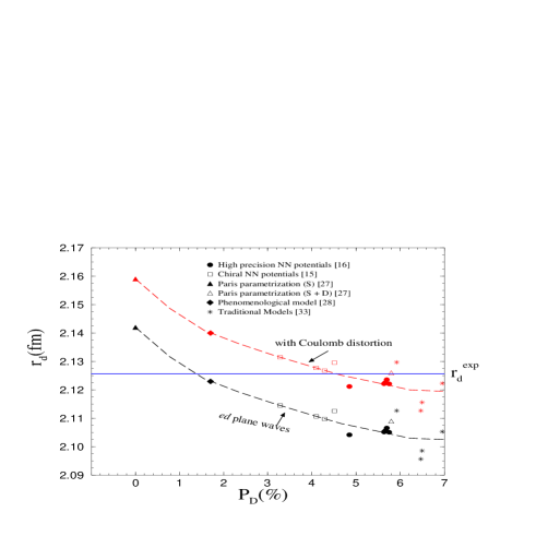
Figure 2: Charge radius of the deuteron as a function of the D-state probability in the deuteron wave function evaluated using different models. The dashed lines are drawn to guide the eye with the red (black) one representing the numbers obtained with (without) the effects of Coulomb distortion included.

In studies of electron-deuteron scattering as in Ref. gilmangross , data have been interpreted in terms of the plane wave Born approximation (PWBA). However, the effects of including distorted $ed$ waves can become important for comparisons with precise data. Noting that the Coulomb distortion sicktrautman changes the deuteron radius by 0.017 fm, the authors in gilmangross suggest an adjustment of the deuteron charge form factor by an amount $\delta G_{C}=-0.003\,+0.104\,Q^{2}$ which decreases the form factor at small $Q^{2}$ and increases the value of the radius. The results presented in Table 1, however, do not take these effects into account since it is not appropriate to evaluate (6) (which involves $V_{d}(r)$ obtained from a Fourier integral over all momenta) using the form factor corrected only at low $Q^{2}$. The correction at low $Q^{2}$ introduces a disagreement with data at large $Q^{2}$ as shown in gilmangross . The above correction is however important for the calculation of the radius defined by the derivative of the form factor at $Q^{2}$ = 0 and hence in Table 2, we present the deuteron charge radius, $r_{d}$, with the Coulomb distortion correction of 0.017 fm as in sicktrautman for different choices of the nucleon-nucleon (NN) potentials. Fig. 2 displays the same with and without the Coulomb distortion included. From the figure we observe a general trend of increasing $P_{D}$ for smaller radii. However, the results are model dependent with the chiral models indicating a value of $P_{D}$ = 4.3 and the high precision NN models a value around 5.7 leading to a good agreement with the experimental $r_{d}=2.12562(78)$ fm pohldeut . The choice of the proton and neutron form factor parametrization (which affects the values of $r_{p}$ and $r_{n}$ entering in $r_{d}^{2}=r_{p}^{2}+r_{n}^{2}+(3/4m_{p}^{2})+(1/4)\,\int_{0}^{\infty}\,[|u(r)|^{2}+|w(r)|^{2}]\,r^{2}dr$), can add a small uncertainty to the values deduced in Table 2. The magnitude of these uncertainties using different parametrizations for $G_{E}^{p}$ and $G_{E}^{n}$ which reproduce the deuteron charge form factor, $G_{ch}(Q)=G_{0}(Q)[G_{E}^{p}(Q^{2})+G_{E}^{n}(Q^{2})][1\,-\,(Q^{2}/8m_{N}^{2})]$ equally well, remains to be investigated in future.

IV Finite size Coulomb plus Darwin corrections at order $\alpha^{4}$

For completeness, we also calculate the FSC with the Darwin terms in (4) within the few body formalism. The Fourier transform of the muon-deuteron interaction potential, $V_{\mu^{-}d}(Q)$, can be done numerically to obtain the potential in coordinate space which can then be used to evaluate the energy correction using first order time independent perturbation theory as,

$$\Delta E=\int|\Psi_{nl}(\bm{r})|^{2}\,\biggl{[}\,V_{\mu^{-}d}(r)\,-V_{\mu^{-}d}(r)^{point}\,\biggr{]}\,d^{3}r\,$$ (8)

where, $\Psi_{nl}(\bm{r})$ is the unperturbed atomic wave function. Note that we have subtracted the point-like contribution $-\alpha/r$ as well as the point-like Darwin terms from $V_{\mu^{-}d}(r)$ so that the quantity in square brackets is the perturbative potential only due to deuteron structure. In Table 3, we list the finite size corrections (FSC) (to the Coulomb and Darwin terms) of order $\alpha^{4}$ in muonic deuterium using Eq. (8) and different percentages of the D-state probabilities in the deuteron wave function for the energy levels with $l=0$ and $n=1,2$. Since the numbers in Table 3 are not very different from those in Table 1 (compare the first line in Table 1 with the second line in Table 3), one can say that the FSC due to the Darwin terms are in general very small.

Table 3: Finite size corrections $\Delta E$ in meV (Eq. (8)), to the 1S and 2S atomic levels in $\mu^{-}d$, for different D-state probabilities of the deuteron wave function.

	7% mcgee	5.8% lacombe	1.7 %berez	0 lacombe
1S	206.28	210.42	213.17	217.19
2S	25.78	26.31	26.65	27.15

Note that Eqs (8) and (6) are different in the sense that (i) $V_{\mu^{-}d}$ in (8) contains the additional muon Darwin term as compared to $e\,V_{d}$ and (ii) whereas (8) subtracts the point-like potential, $V_{\mu^{-}d}(r)^{point}$, which contains the point-like Coulomb term, $-4\pi\alpha/r$ and two point-like Darwin terms $\delta^{3}(\bm{r})/8M_{N}^{2}$ and $\delta^{3}(\bm{r})/8M_{\mu}^{2}$, Eq. (6) subtracts only the point-like Coulomb, $-4\pi\alpha/r$.

To summarize, the leading order nuclear structure corrections in muonic deuterium have been evaluated within a few body formalism which reveals the dependence of the correction on the model of the deuteron wave function. Since scattering data do not have the high precision achieved by the muonic atom spectroscopy data, the deuteron charge form factor can be reproduced equally well (within error bars) by all the parametrizations of the deuteron wave function used, irrespective of the percentage of $P_{D}$ in them. However, we notice that a comparison of the radius evaluated using these parametrizations with the precise radius value extracted from $\mu^{-}d$ spectroscopy provides a complementary tool to determine $P_{D}$. Though there do exist model dependent uncertainties in $P_{D}$ (see Table 2 and Fig. 2), there seems to be a general trend of increasing values of $P_{D}$ for smaller $r_{d}$. The few body formalism presented here can also be used to evaluate the nuclear structure corrections in muonic helium atoms which are expected to be studied in future.

Acknowledgments
One of the authors (D. B. F.) thanks the administrative department of science, technology and innovation of Colombia (COLCIENCIAS) and the Faculty of Science, Universidad de los Andes for the financial support provided. He is also grateful to IFIC, University of Valencia and Prof. Vicente Vacas for their kind hospitality and useful discussions.

References

- (1) H. Feshbach and J. Schwinger, Phys. Rev. 84, 194 (1951).
- (2) N. L. Rodning and L. D. Knutson, Phys. Rev. Lett. 57, 2248 (1986); ibid, Phys. Rev. C 41, 898 (1990).
- (3) J. A. Oller, Phys. Rev. C 93, 024002 (2016).
- (4) R. D. Amado, Phys. Rev. C 19, 1473 (1979); J. L. Friar, Phys. Rev. C 20, 325 (1979).
- (5) H. E. Conzett et al., Phys. Rev. Lett. 43, 572 (1979).
- (6) E. Hadjimichael, Nucl. Phys. A 312, 341 (1978).
- (7) L. Mathelitsch and H. F. K. Zingl, Il Nuovo Cimento 44, 81 (1978).
- (8) J. S. Levinger, Phys. Lett. B 29, 216 (1969).
- (9) R. Pohl et al., Science 353, 669 (2016).
- (10) W. Leidemann and R. Rosenfelder, Phys. Rev. C 51, 427 (1995).
- (11) K. Pachucki, Phys. Rev. Lett. 106, 193007 (2011); K. Pachucki and A. Wienczek, Phys. Rev. A 91, 040503(R) (2015).
- (12) O. J. Hernandez et al., Phys. Lett. B 736, 344 (2014).
- (13) J. L. Friar, Annals of Phys. 122, 151 (1979).
- (14) J. L. Friar, Phys. Rev. C 88, 034003 (2013).
- (15) D. R. Entem and R. Machleidt, Phys. Rev. C 68, 041001 (2003); E. Epelbaum, W. Göckle and U. -G. Meissner, Nucl. Phys. A 747, 362 (2005); E. Epelbaum, H. Krebs and U. -G. Meissner, Phys. Rev. Lett. 115, 122301 (2015); D. R. Entem, R. Machleidt and Y. Nosyk, preprint, arXiv:1703.05454 (2017).
- (16) V. C. J. Stoks, R. A. M. Klomp, C. P. F. Terheggen and J. J. de Swart, Phys. Rev. C 49, 2950 (1994); R. Machleidt, Phys. Rev. C 63, 024001 (2001); R. B. Wiringa, V. C. J. Stoks and R. Schiavilla, Phys. Rev. C 51, 38 (1995).
- (17) D. Bedoya Fierro, N. G. Kelkar and M. Nowakowski, JHEP 1509, 215 (2015); N. G. Kelkar, F. Garcia Daza and M. Nowakowski, Nucl. Phys. B 864, 382 (2012).
- (18) F. Garcia Daza, N. G. Kelkar and M. Nowakowski, J. Phys. G 39 035103 (2012).
- (19) H. B. G. Casimir and P. Polder, Phys. Rev. 73 (1948) 360; E.M. Lifschitz, JETP Lett.2 (1956) 73; F. Ferrer and J. A. Grifols, Phys. Lett. B460, 371, 1999.
- (20) R. Machleidt, Adv. Nucl. Phys. 19, 181 (1989); J. D. Walecka, Theoretical Nuclear and Subnuclear physics, Second Edition, World Scientific 2004.
- (21) V. B. Belyaev, Lectures on the theory of few body systems, Springer-Verlag (Heidelberg, 1990); S. A. Rakityansky eta al., Phys. Rev. C 53, R2043 (1996).
- (22) N. G. Kelkar, Phys. Rev. Lett. 99, 210403 (2007).
- (23) J. L. Friar and J. W. Negele, Advances in Nuclear Physics 8, pp. 219-376, Springer, New York (1975); J. L. Friar, J. Martorell and D. W. L. Sprung, Phys. Rev. A 56, 4579 (1997).
- (24) J. J. Krauth et al., Ann. Phys. 366, 168 (2016).
- (25) R. Gilman and F. Gross, J. Phys. G. 28, R37 (2002).
- (26) H. Arenhövel, F. Ritz and T. Wilbois, Phys. Rev. C 61, 034002 (2000).
- (27) M. Lacombe et al., Phys. Lett. B 101, 139 (1981).
- (28) Yu. A. Berezhnoy, V. Yu Korda and A. G. Gakh, Int. J. Mod. Phys. E 14, 1073 (2005).
- (29) I. J. McGee, Phys. Rev. 151, 772 (1966).
- (30) D. Abbott et al., Eur. Phys. J. A 7, 421 (2000).
- (31) C. Itzykson and J.-B. Zuber, Quantum Field Theory, Dover Publications, New York (1980).
- (32) I. Sick and D. Trautmann, Phys. Lett. B 375, 16 (1996); ibid, Nucl. Phys. A 637, 559 (1998); I. Sick, Prog. Part. Nucl. Phys. 47, 245 (2001).
- (33) Roderick V. Reid Jr., Ann. Phys. 50, 411 (1968); J. W. Humberston and J. B. G. Wallace, Nucl. Phys. A 141, 362 (1970); R. De Tourreil, B. Rouben and D. W. L. Sprung, Nucl. Phys. A 242, 445 (1975).