Mesoscopic fluctuations in biharmonically driven flux qubits

Abstract

We investigate flux qubits driven by a biharmonic magnetic signal, with a phase lag that acts as an effective time reversal broken parameter. The driving induced transition rate between the ground and the excited state of the flux qubit can be thought as an effective transmitance, profiting from a direct analogy between interference effects at avoided level crossings and scattering events in disordered electronic systems. For time scales prior to full relaxation but large compared to the decoherence time, this characteristic rate has been accessed experimentally and its sensitivity with both the phase lag and the dc flux detuning explored. In this way signatures of Universal Conductance Fluctuations-like effects have recently been analized in flux qubits and compared with a phenomenological model that only accounts for decoherence, as a classical noise. We here solve the full dynamics of the driven flux qubit in contact with a quantum bath employing the Floquet Markov Master equation. Within this formalism relaxation and decoherence rates result strongly dependent on both the phase lag and the dc flux detuning. Consequently, the associated pattern of fluctuations in the characteristic rates display important differences with those obtained within the mentioned phenomenological model. In particular we demonstrate the Weak Localization-like effect in the averages values of the relaxation rate. Our predictions can be tested for accessible, but longer time scales than the current experimental times.

I Introduction

The quantum conductance of a phase coherent conductor can be related, in the diffusive regime, to the transmission probability through the disordered region.datta For milikelvin temperatures, when typically the coherence length could become larger than the scattering mean free path, the interference term present in the transmission probability survives disordered averaging, giving rise to quantum corrections to the classical transport properties and novel phenomena. Mesoscopic effects like Weak Localization and Universal Conductance Fluctuations have been predicted and extensively tested in electronic quantum system for years.varios_ucf ; varios_wl ; leshouches

Universal conductance fluctuations (UCF) are sample to sample fluctuations- of the order of the quantum of conductance- originated on the sensitivity of the quantum conductance to changes in an external parameter, like a magnetic flux or a gate voltage.varios_ucf

The Weak localization (WL) effect is a quantum correction to the classical conductance, that survives disorder averaging when time reversal symmetry is present.varios_wl Without spin-orbit effects, it is characterized by a dip in the conductance (peak in the resistance) at zero magnetic field. The standard way to detect the WL effect is by its suppression, as its strength falls off with an applied magnetic field. A critical field that scales as $B_{c}\sim 1/(D\tau_{\phi})$, with $D$ the diffusion coefficient and $\tau_{\phi}$ the coherence time, washes out the quantum interference term, and thus the WL correction. varios_wl The measurement of $B_{c}$ has been established as a usual route to determine the coherence time. varios_wl ; leshouches

Flux qubits (FQ) are model artificial atoms whose energy levels can be manipulated by an external magnetic flux. qbit_mooij ; chiorescu For most of the applications in quantum information theory, only the two lowest energy levels of the FQ have been considered in studies of their quantum dynamics.chiorescu However, FQ exhibits as a function of the static magnetic flux a complex structure of energy levels with multiple avoided crossings. This rich spectrum can be explored by driving the FQ with an ac magnetic flux, for moderate driving frequencies - in the microwave range. In a typical protocol, the FQ is initially prepared in its ground state for a given value of the dc flux, and evolves under the ac driving quasi adiabatically until the first avoided crossing is reached. There, the state obeys a Landau-Zener-Stückelberg (LZS) transition and transforms into a coherent superposition of the ground and excited states.oliver ; nori2011 For weak ac amplitudes, such that a single avoided crossing is reached by the driving protocol, the superposition state and the initial one interfere again at the second passage for the avoided crossing. Hence, the avoided crossing acts as an effective beam splitter, where scattering events take place. For driving periods larger than the coherence time, the evolved state accumulates a total phase, that depends both on the dc flux and the driving amplitude.oliver ; nori2011 .

The regime of weak driving, when only the lowest two energy levels of the FQ are explored and a single avoided crossing is attained by the amplitude of the ac flux, has been studied in extent both experimentally and theoretically. oliver ; ferron ; gustavsson In this way, FQ have been investigated extensively in recent years as high resolution Mach-Zhender type of interferometers. oliver

For large driving amplitudes, when many avoided crossings can be reached, the repeated sweeps through the avoided level crossings result in successive LZS transitions between different energy levels. This driving protocol -named as amplitude spectroscopy (AS) oliver - was employed to reconstruct the FQ energy level spectrum and to study its dynamics under different conditions. valenzuela ; fds The AS protocol has been also successfully applied in other systems like charge qubits cqubits , ultracold molecular gases mark and single electron spins. huang

The interaction of the driven FQ with an external bath has been recently studied to incorporate more realistic dissipative scenarios beyond the pure coherent regime. Relevant and potential useful phenomena like population inversion, sun2009 ; hanggi ; ferron_prl dynamical transition in the interference patterns, ferron_arx and estimates for coherence times have been extracted from these studies.shevchenko ; dupont2013

While a priori there is not a direct connection between driven FQ and mesoscopic disordered electronic systems, the identification of a transition at the avoided crossing as a scattering event, suggests a route to study mesoscopic-like effects in driven FQ. However, for the weak driving regime at most one avoided crossing is reached by the protocol and only two scattering events (transitions) take place in one period of the driving. This poor scattering regime seems insufficient to explore the mesoscopic analogy.

An alternative was proposed in Ref.gustavsson, with the implementation of a protocol generated by a biharmonic flux with a phase lag. The signal was designed to drive the FQ up to four times through the avoided crossing in one period, which was chosen much shorter than the energy relaxation time. Therefore, after many periods of the driving the excited state of the FQ was populated as a function of time with a characteristic (equilibration) rate that was extracted in the experiment by a fitting procedure.

Other interesting phenomena of biharmonic drive in flux qubits have been studied in recent experimental bylan2009 ; forster2015 and theoretical satanin2014 ; blattmann2015 works.

The interference conditions can be changed by either tuning the external dc flux or the phase lag in the driving wave form. Following this strategy, the equilibration rate $\Gamma$ and its concomitant fluctuations have been analyzed in Ref. gustavsson, .

For large driving frequencies and for time scales smaller than the relaxation time but larger than the decoherence time, it is possible to study the dynamics of the FQ within a model of classical diagonal noise and computing $\Gamma$ from phenomenological rate equations.lt Neglecting relaxation, it can be shown that $\Gamma\sim 2W$, with $W$ the transition rate induced by driving. lt The mesoscopic analogy proposed in Ref.gustavsson, was to identify $W$ with a transmission rate, which in (mesoscopic) electronic transport determines the conductance. datta Thus the goal was to access the fluctuations in $W$ through the study of the fluctuations in $\Gamma$. This scenario, although tempting, should be taken with caution.

As we already mentioned, the expression $\Gamma\sim 2W$ is valid for large driving frequencies and for time scales far below relaxation. berns ; gustavsson

We solve the full dynamics of the driven FQ employing the Floquet Markov (FM) master equation to include relaxation and decoherence processes for a realistic model of a quantum bath.hanggi ; ferron_prl ; ferron_arx This formalism floquet , valid for arbitrary time scales and strength of the driving protocol, allows to compute the decoherence and the relaxation (equilibration) rates. As we will show, both rates result strongly dependent on the driving amplitude and the dc flux, attaining values that might differ up to an order of magnitude from those determined in the absence of driving. Consequently, the relaxation (equilibration) rate obtained within the FM formulation might strongly differ from the value $2W$ - used in Ref.gustavsson, to compare with the experimental results-.

An important outcome of our study is related to the weak localization (WL) effect, which was not resolved in the experiment of Ref.gustavsson, . As we will analize, it is not the driving protocol but the accessible decoherence time which limits the detection of the effect. gustavsson . In fact, the WL correction could be measured in the regime of larger coherence times.

The paper is organized as follows. In Sec. II we review the Hamiltonian model for the flux qubit (FQ) and the effective Hamiltonian obtained when only the two lowest levels of the FQ are considered. In Sec.III.1 we derive an analytical expression for the rate $\Gamma$ obtained within a phenomenological approach which includes classical noise as the only source of decoherence. Gaussian and low frequency type of noise are both considered. paladino .

Due to the limitations of the analytical approach, already mentioned, we implement in Sec.III.2 the full quantum mechanical calculation in order to obtain the equilibration (relaxation) rate $\Gamma_{r}$ within the Floquet Markov (FM) master equation. The last part of this section is devoted to compare the behavior of $\Gamma\sim 2W$ and $\Gamma_{r}$ as a function of the dc flux, and to analize the effect that the driving has on the determination of both decoherence and relaxation rates. The fluctuations in the rates $\Gamma\sim 2W$ and $\Gamma_{r}$ as a function of the dc flux and the time reversal parameter are analized in Sec.IV. As we show, besides UCF, clear signatures of WL correction could be also detected if the coherence is increased. We discuss the limitation imposed by the accessible decoherence time in the experimental determination of the WL correction. We conclude in Sec.V with a discussion and perspectives.

II The flux qubit

The Flux qubit (FQ) consists on a superconducting ring with three Josephson junctionsqbit_mooij enclosing a magnetic flux $\Phi=f\Phi_{0}$, with $\Phi_{0}=h/2e$. Two of the junctions have the same Josephson coupling energy $E_{J,1}=E_{J,2}=E_{J}$, and capacitance, $C_{1}=C_{2}=C$, while the third one has smaller coupling $E_{J,3}=\alpha E_{J}$ and capacitance $C_{3}=\delta C$, with $0.5<\delta<1$. The junctions have gauge invariant phase differences defined as $\varphi_{1}$, $\varphi_{2}$ and $\varphi_{3}$, respectively. Typically the circuit inductance can be neglected and the phase difference of the third junction is: $\varphi_{3}=-\varphi_{1}+\varphi_{2}-2\pi f$.

Therefore, the system can be described in terms of two independent dynamical variables, chosen as $\varphi_{l}=(\varphi_{1}-\varphi_{2})/2$ (longitudinal phase) and $\varphi_{t}=(\varphi_{1}+\varphi_{2})/2$ (transverse phase). In terms of these variables, the hamiltonian of the FQ (in units of $E_{J}$) is: qbit_mooij

$${\cal H}_{FQ}=-\frac{\eta^{2}}{4}\left(\frac{\partial^{2}}{\partial\varphi_{t}^{2}}+\frac{1}{1+2\delta}\frac{\partial^{2}}{\partial\varphi_{l}^{2}}\right)+V(\varphi_{l},\varphi_{t})\;,$$ (1)

with $\eta^{2}=8E_{C}/E_{J}$ and $E_{C}=e^{2}/2C$. The kinetic term corresponds to the electrostatic energy of the system and the potential one to the Josephson energy of the junctions, given by $V(\varphi_{l},\varphi_{t})=2+\delta-2\cos\varphi_{t}\cos\varphi_{l}-\delta\cos(2\pi f+2\varphi_{l})$. Typical FQ experiments have values of $\delta$ in the range $0.6-0.9$ and $\eta$ in the range $0.1-0.6$. chiorescu ; valenzuela It is operated at magnetic fields near the half-flux quantum, qbit_mooij ; chiorescu $f=1/2+f_{0}$, with $f_{0}\ll 1$. For $\delta\geq 1/2$, the potential $V(\varphi_{l},\varphi_{t})$ has two minima at $(\varphi_{l},\varphi_{t})=(\pm\varphi^{*},0)$ separated by a maximum at $(\varphi_{l},\varphi_{t})=(0,0)$. Each minima corresponds to macroscopic persistent currents of opposite sign, and for $f\gtrsim 1/2$ ($f\lesssim 1/2$) a ground state $|+\rangle$ ($|-\rangle$) with positive (negative) loop current is favoured.

For values of $|f_{0}|\ll 1$, such that the avoided crossings with the third energy level are not reached, the hamiltonian of Eq. (1) can be reduced to the two-level system (TLS)qbit_mooij ; ferron

$${\cal H}=-\frac{\varepsilon_{0}}{2}{\hat{\sigma}}_{z}-\frac{\Delta}{2}{\hat{\sigma}}_{x}\;,$$ (2)

in the basis defined by the persistent current states $|\pm\rangle=(|0\rangle\pm|1\rangle)/\sqrt{2}$, with $\hat{\sigma}_{z}$, $\hat{\sigma}_{x}$ the Pauli matrices and $|0\rangle$ and $|1\rangle$ the ground and excited states at $f_{0}=0$. The parameters of ${\cal H}$ are the gap (at $f_{0}=0$) $\Delta$ and the detuning energy $\varepsilon_{0}=4\pi I_{p}f_{0}$. Here $I_{p}=\delta|\langle+|\sin 2\varphi_{l}|+\rangle|=\delta|\langle-|\sin 2\varphi_{l}|-\rangle|$ is the magnitude of the loop current, which for our case with $\delta=0.8$ and $\eta=0.25$ is $I_{p}=0.721$ (in units of $I_{c}=2\pi E_{J}/\Phi_{0}$).

Figure 1 sketches the energy levels diagram for the FQ hamiltonian restricted to the TLS, Eq.(2) with $E_{0,1}=\pm 1/2\sqrt{\varepsilon_{0}^{2}+\Delta^{2}}$ the ground and excited states energies, respectively. oliver ; valenzuela ; berns .

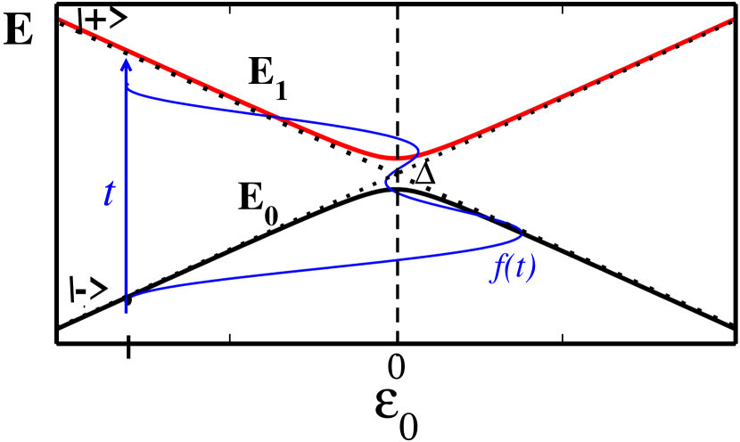
Figure 1: (color online) Flux Qubit energy diagram for the TLS hamiltonian Eq.(2), as a function of flux detuning $\varepsilon_{0}$. Inset: implemented biharmonic pulse $f(t)$, chosen to drive the FQ four times through the avoided crossing in one period.

The FQ restricted to weak driving amplitudes was the regime explored in Ref.gustavsson, . Consistently, in the following we focus on the dynamics of the TLS Hamiltonian Eq.(2) under the effect of the biharmonic driving.

III Two level system under biharmonic driving

III.1 Equilibration rate within the classical noise model

As we mentioned, in Ref.gustavsson, the equilibration rate $\Gamma$ is experimentally determined by fitting the decay of the excited population to the equilibrium, assuming an exponential behavior as a function of time.

In the following we describe a route to compute $\Gamma$ from phenomenological rate equations in the regime of large driving frequencies, for which the change in the qubit population (per unit time) induced by the driving is small compared to the decoherence rate $\Gamma_{2}\equiv 1/T_{2}$ but large compared to the inelastic relaxation rate in the absence of driving, $\Gamma_{1}\equiv 1/T_{1}$. As the calculation is adapted from the one derived for the single driving protocol berns we here present the main steps stressing differences. The source of noise is considered classical and diagonal, which essentially means that the noise produces pure dephasing. However diagonal noise is consistent with the typical experimental situation with FQ where the dominant source of noise is flux-like.

From phenomenological rate equations the equilibration rate can be written as $\Gamma=2W+\Gamma_{1}$ , with $W$ the transition rate induced by the driving protocol.berns For large relaxation times $T_{1}$ and for $W\gg\Gamma_{1}$, one gets $\Gamma\approxeq 2W$. Larger values of $\Gamma_{1}$ would require the explicit inclusion of relaxation processes in the analysis to avoid important differences between $W$ and $\Gamma$. These cases will be addressed in Sec.III.2.

To compute $W$, we include in Eq.(2) the time dependent biharmonic driving and the diagonal classical noise by replacing $\varepsilon_{0}\rightarrow h(t)=\varepsilon_{0}+\delta\varepsilon+\varepsilon(t)$. The term $\varepsilon(t)=4\pi I_{p}f(t)$, contains the biharmonic ac flux $f(t)=A_{1}\cos{(\omega_{0}t+\alpha)}-A_{2}\cos{(2\omega_{0}t)}$ of fundamental frequency $\omega_{0}=2\pi/\tau$. The phase lag $\alpha$ turns the protocol asymmetric in time and the amplitudes ratio $A_{1}/A_{2}$ was chosen to drive the FQ up to four times through the avoided crossing in one period $\tau$. The classical noise is $\delta\varepsilon$.

The Hamiltonian Eq.(2) can be turned to purely off-diagonal becoming, after an unitary transformation (we use $\hbar=1$),

$$\tilde{{\cal H}}=-\frac{\Delta^{\ast}(t)}{2}\hat{\sigma}_{x}\;,$$

where $\Delta(t)=\Delta e^{-i\phi(t)}$ and $\phi(t)=\int_{0}^{t}h(t^{\prime})dt^{\prime}$.

The FQ is usually initially prepared in its ground state, $|\Psi_{g}(t=0)\rangle$, for a given value of the detuning $\varepsilon_{0}$ (in Fig.1 an initial state for $\varepsilon_{0}<0$ is chosen). Alternatively it is possible to initialize the FQ in an eigenstate of the computational basis, i.e. $|-\rangle$($|+\rangle$) for $\varepsilon_{0}<0$ ($\varepsilon_{0}>0$). In general, for values of flux detuning $\varepsilon_{0}>\Delta$, the initial state satisfies $|\Psi_{g}(t=0)\rangle\longrightarrow|-\rangle(|+\rangle)$ for $\varepsilon_{0}<0(\varepsilon_{0}>0)$.

The transition rate $W$ induced by the driving is the time derivative of the transition probability between the initial and the final state. Under the assumption of fast driving, $\omega_{0}=2{\pi/\tau}>\Delta$, it can be computed expanding the time evolution operator to first order in $\Delta$,

$$U(t,0)=1-i\int_{0}^{t}\tilde{{\cal H}}(\tau)d\tau+{\cal O}({\Delta^{2}})\;.$$

Therefore we write:

$$W=\frac{d}{dt}|\langle+|U(t,0)|-\rangle|^{2}=\frac{d}{dt}\frac{1}{4}\int_{0}^{t}\int_{0}^{t}\Delta(\tau_{1})\Delta^{\ast}(\tau_{2})d\tau_{1}d\tau_{2}\;$$

$$=\frac{d}{dt}\frac{\Delta^{2}}{4}\int_{0}^{t}\int_{0}^{t}{\Re}\{\exp-i\left(\phi(\tau_{1})-\phi(\tau_{2})\right)\}d\tau_{1}d\tau_{2},$$ (3)

with $\Re\{..\}$ the real part.

In the above integrand we define

$$e^{-i\phi(t)}=e^{-i\varepsilon_{0}t-i\delta\phi(t)}\sum_{nm}J_{n}(x_{1})e^{in(\omega_{0}t+\alpha)}J_{m}(x_{2})e^{-i2m\omega_{0}t}\,,$$ (4)

where we have used the expansion of $\exp(ix\sin u)=\sum_{p}J_{p}(x)\exp(-ipu)$ in terms of Bessel functions of first kind. We also defined $x_{1}=A_{1}/\omega_{0}$ and $x_{2}=A_{2}/(2\omega_{0})$.

For a gaussian white noise, the correlator is $\langle\delta\varepsilon(t)\delta\varepsilon(t^{\prime})\rangle=2\Gamma_{2}\delta(t-t^{\prime})$. As $\delta\phi(t)=\int_{0}^{t}\delta\varepsilon(\tau)d\tau$, we take the average over noise in Eq.(III.1) using $\langle e^{i\delta\phi(t)}e^{-i\delta\phi(t^{\prime})}\rangle=e^{-\Gamma_{2}|t-t^{\prime}|}$, with $\Gamma_{2}$ the decoherence (pure dephasing) rate for this model of classical diagonal noise.

The next step is to perform the time integration in Eq.(III.1), getting

$$W=\frac{\Delta^{2}\Gamma_{2}}{2}{\Re}\{\sum_{nn^{\prime}mm^{\prime}}\lambda_{nn^{\prime}mm^{\prime}}\times$$

$$\frac{e^{i(n-n^{\prime})\alpha}e^{i\omega_{0}(n-n^{\prime})t}e^{2i\omega_{0}(m^{\prime}-m)t}}{(\varepsilon_{0}+(2m-n)\omega_{0})^{2}+\Gamma_{2}^{2}}\;\},$$ (5)

with $\lambda_{nn^{\prime}mm^{\prime}}\equiv J_{n}(x_{1})J_{n^{\prime}}(x_{1})J_{m}(x_{2})J_{m^{\prime}}(x_{2})$.

Under the fast driving regime, the non zero exponents are highly oscillating compared to the time scale of the driving. Therefore we only keep the contributions with $\omega_{0}(n-n^{\prime})+2\omega_{0}(m^{\prime}-m)=0$, and the transition rate reads:

$$W=\frac{\Delta^{2}\Gamma_{2}}{2}\sum_{nn^{\prime}mm^{\prime}}\frac{\lambda_{nn^{\prime}mm^{\prime}}\cos{((n-n^{\prime})\alpha)}}{(\varepsilon_{0}+(2m-n)\omega_{0})^{2}+\Gamma_{2}^{2}}\delta_{n-n^{\prime},2(m-m^{\prime})}.$$ (6)

Equation (6) exhibits an explicit dependence on the phase lag $\alpha$, and a lorentzian line shape close to the resonance condition $\varepsilon_{0}=(n-2m)\omega_{0}$, which is characteristic of white noise models in the regime of times $t\ll T_{1}$. For $x_{2}=0$ , Eq.(6) reduces to the expression of the transition rate obtained for single driving protocols.amin ; berns

In Fig.2 we plot $2W$ obtained from Eq.(6) as a function of the static flux detuning $\varepsilon_{0}$, for the symmetric driving, $\alpha=0$, in Fig.2(a) and for $\alpha=0.2$ in Fig.2(b). The FQ parameters are $\Delta/h=19\,$ MHz, $\omega_{0}/(2\pi)=125\,$ MHz, $A_{1}=3\,m\Phi_{0}$ and $A_{2}=1.65\,m\Phi_{0}$, identical to those reported in the experiment of Ref.gustavsson, . The salient feature is that the peaks are not symmetric with $\varepsilon_{0}$, exhibiting a more fluctuating pattern of resonances for $\varepsilon_{0}<0$. This is a manifestation of the sensitivity of the total accumulated phase in one period of the driving with $\varepsilon_{0}$ and $\alpha$. We have chosen the same amplitudes ratio $A_{2}/A_{1}=0.55$ as in Ref.gustavsson, , selected to drive the FQ up to four times through the avoided crossing in one driving period $\tau$, in the range of negative detunings $\varepsilon_{0}<0$ (see Fig. 1). The strong fluctuating pattern is due to the three different phases (one phase for two successive passages) and eight possible superposition states that arises as $\varepsilon_{0}$ is varied. For other values of $\varepsilon_{0}$, the waveform traverses the avoided crossing zero or two times per cycle, producing no accumulated phase or a single one, with interference conditions that originate a smoother behaviour of $\Gamma$ with $\varepsilon_{0}$.

As expected, the resonance peaks decrease and turn wider as the dephasing rate $\Gamma_{2}$, included in Eq.(6) as a parameter, is increased. This is fully consistent with the transition from the non overlapping to the overlapping resonances limit, also observed experimentally for the single harmonic driving protocols. oliver ; valenzuela

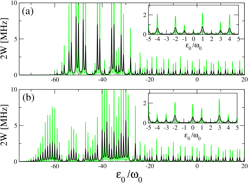
Figure 2: (color online) Rate $2W$ obtained from Eq.(6) for FQ parameters $\Delta/h=19\,$ MHz, $\omega_{0}/(2\pi)=125\,$ MHz, $A_{1}=3\,m\Phi_{0}$, $A_{2}=1.65\,m\Phi_{0}$, for $\Gamma_{2}=100\,$ MHz (black line) and $\Gamma_{2}=30\,$ MHz (green line). (a) $\alpha=0$ , (b) $\alpha=0.2$. The insets show a magnification of selected resonances.

The derivation can be adapted to consider other spectral functions with Gaussian noise. In the case of FQ, the magnetic flux noise in SQUIDS could have a spectral density $S(\omega)$, which for low frequencies behaves as $1/\omega^{p}$ noise. paladino ; amin For this case, we get for the transition rate:

$$W_{lf} =\Delta^{2}\sqrt{\frac{\pi}{8\Gamma_{2}}}\sum_{nn^{\prime}mm^{\prime}}\lambda_{nn^{\prime}mm^{\prime}}\cos{((n-n^{\prime})\alpha)}\times$$

$${\exp\{\frac{-(\varepsilon_{0}+(2m-n)\omega_{0})^{2}}{\Gamma_{2}}\}}\;.$$

where $\Gamma_{2}=\int S(\omega)d\omega$ is assumed finite, and we define $W_{lf}$ as the transition rate induced by driven in the presence of low frequency noise. Notice that the main effect of a noise with a low frequency part is to modify the lorentzian line shape of the individual resonances by a Gaussian line shape.

In Ref.gustavsson, , the transition rate induced by driving $W$ was fully identified with the equilibration rate $\Gamma$ (up to a factor 2). As we anticipated, this requires of values $W<\Gamma_{2}$, and time scales $t\ll T_{1}=1/\Gamma_{1}$.

We will show in the next section that new characteristics emerge in the behaviour of the equilibration rate when the full dynamics, including quantum noise, is considered within the Floquet Markov approach. In particular, we will analyse the behavior and sensitivity of the decoherence and relaxation rates with the flux detuning. The strong variations that these two rates experience close to resonances with the driving field, question the results of this section for times scales close to full relaxation.

III.2 Equilibration rate within the Floquet Markov Master Equation

We start this section by reviewing the main ingredients of the Floquet Markov formalism, and for further details we suggest the Appendix of Ref.ferron_arx, .

Since the FQ is driven with a biharmonic magnetic flux $f(t)=A_{1}\cos{(\omega_{0}t+\alpha)}-A_{2}\cos{(2\omega_{0}t)}$, its hamiltonian is time periodic ${\cal H}(t)={\cal H}(t+\tau)$, with $\tau=2\pi/\omega_{0}$. In the Floquet formalism, which allows to treat periodic forces of arbitrary strength and frequency floquet ; fds ; ferron_prl ; ferron_arx , the solutions of the Schrödinger equation are of the form $|\Psi_{\beta}(t)\rangle=e^{i\mu_{\beta}t/\hbar}|\beta(t)\rangle$, where the Floquet states $|\beta(t)\rangle$ satisfy $|\beta(t)\rangle$=$|\beta(t+\tau)\rangle=\sum_{k}|\beta_{k}\rangle e^{-ik\omega_{0}t}$, and are eigenstates of the equation $[{\cal H}(t)-i\hbar\partial/\partial t]|\beta(t)\rangle=\mu_{\beta}|\beta(t)\rangle$, with $\mu_{\beta}$ the associated quasi-energy.

Experimentally, the FQ is affected by the electromagnetic environment that introduces decoherence and relaxation processes. A standard theoretical model to cope with these effects, is to linearly couple the system to a bath of harmonic oscillators with a spectral density $J(\omega)$ and equilibrated at temperature $T$.hanggi ; milenas ; grifonih ; caspar For the FQ the dominating source of noise is flux-like, in which case the bath degrees of freedom couple with the system variable $\varphi_{l}$ caspar ; ferron_arx In the two-level representation of Eq.(2), the flux noise is usually represented by a system bath hamiltonian of the form $H_{sb}\propto\sigma_{z}$. milenas

For weak coupling (Born approximation) and fast bath relaxation (Markov approximation), a Floquet-Born-Markov master equation for the reduced density matrix $\hat{\rho}$ in the Floquet basis, $\rho_{\alpha\beta}(t)=\langle\alpha(t)|\hat{\rho}(t)|\beta(t)\rangle$, can be obtained.hanggi

Considering that the time scale $t_{r}$ for full relaxation satisfied $t_{r}\gg\tau$, one gets (see Appendix of Ref.ferron_arx, for details):

$$\frac{d\rho_{\alpha\beta}(t)}{dt}=-\frac{i}{\hbar}(\mu_{\alpha}-\mu_{\beta})\rho_{\alpha\beta}(t)+\sum_{\alpha^{\prime}\beta^{\prime}}{\it L}_{\alpha^{\prime}\beta^{\prime}\alpha\beta}\;\rho_{\alpha^{\prime}\beta^{\prime}}(t)\;.$$ (8)

The first term in Eq.(8) represents the non dissipative dynamics and the influence of the bath is described by the rate coefficients averaged over one period of the driving $\tau$, ferron_arx

$${\it L}_{\alpha\beta\alpha^{\prime}\beta^{\prime}} = R_{\alpha\beta\alpha^{\prime}\beta^{\prime}}+R_{\beta\alpha\beta^{\prime}\alpha^{\prime}}^{*}$$

$$-\sum_{\eta}\left(\delta_{\beta\beta^{\prime}}R_{\eta\eta\alpha^{\prime}\alpha}+\delta_{\alpha\alpha^{\prime}}R_{\eta\eta\beta^{\prime}\beta}^{*}\right).$$

The rates

$$R_{\alpha\beta\alpha^{\prime}\beta^{\prime}}=\sum_{q}g_{\alpha\alpha^{\prime}}^{q}A_{\alpha\alpha^{\prime}}^{q}A_{\beta^{\prime}\beta}^{-q}\;,$$ (10)

can be interpreted as sums of $q$-photon exchange terms and contains information on the system-bath coupling operator $A_{\alpha\beta}^{q}=\sum_{nm}\sum_{k}\alpha_{k,n}^{*}\beta_{k+q,m}\langle n|\varphi_{l}|m\rangle$ written down in terms of the eigenbasis $|n\rangle$ of the FQ Hamiltonian for the undriven case, Eq.(1), with $\alpha_{k,n}=\langle n|\alpha_{k}\rangle$. The nature of the bath is encoded in the coefficients $g_{\alpha\beta}^{q}=J(\mu_{\alpha\beta}^{q}/{\hbar})n_{\rm th}(\mu_{\alpha\beta}^{q})$ with $\mu_{\alpha\beta}^{q}=\mu_{\alpha}-\mu_{\beta}+q\hbar\omega_{0}$ and $n_{\rm th}(x)=1/(\exp{(x/k_{B}T)}-1)$. Here we consider the FQ in contact with an Ohmic bath with a spectral density $J(\omega)=\gamma\omega$ (with a cutoff frequency), defining $J(-x)=-J(x)$ for $x<0$, but other spectral densities could be included.ferron_arx

The Floquet Markov formalism has been extensively employed to study relaxation and decoherence in double-well potentials and two level systems driven by single frequency periodic evolutions . hanggi ; grifoni-hanggi ; breuer ; ketzmerick ; grifonih More recently we applied it to analyze the FQ under strong harmonic driving ferron_prl ; ferron_arx , when many energy levels have to be taken into account.

As in the present work the dynamics of the FQ under a weak biharmonic driving protocol is studied, in the following the FQ Hamiltonian will be reduced to its lowest two levels, Eq. (2).

For large times scales, it is usually assumed that the density matrix becomes approximately diagonal in the Floquet basis grifonih . This approximation is justified when $\mu_{\alpha}-\mu_{\beta}\gg{\it L}_{\alpha^{\prime}\beta^{\prime}\alpha\beta}$, which is fulfilled for very weak coupling with the environment and away from resonances.breuer ; ketzmerick ; fazio1 ; ferron_arx However, to compute fluctuation effects it is necessary to sweep in the dc flux detuning $\epsilon_{0}$, attaining near resonances quasi degeneracies, i.e. $\mu_{\alpha}-\mu_{\beta}\sim 0$. Therefore as the dynamics of the diagonal and off-diagonal density matrix can not be separated, we have to solve the full Floquet Markov equation, Eq.(8), to find relaxation and decoherence rates close to resonances .

The rates are extracted from the non zero eigenvalues of the matrix $\hat{\Lambda}$, given from its entries in the Floquet basis, ${\it L}_{\alpha\beta\alpha^{\prime}\beta^{\prime}}$, defined in Eq.(III.2). The long time relaxation rate $\Gamma_{r}=1/t_{r}$ is the minimum real eigenvalue (excluding the eigenvalue $0$). In addition, the decoherence rate $\Gamma_{ab}$ is given by the negative real part of the complex conjugate pairs of eigenvalues of $\hat{\Lambda}$.ferron_arx

The sensitivity of both rates, $\Gamma_{ab}$ and $\Gamma_{r}$, on the dc flux detuning and the driving amplitude has been analyzed in recent studies of the phonomena of population inversion and dynamic transitions in the LZS interference patters of (single) driven FQ. Both phenomena emerge away from resonances, in the long time regime. ferron_prl ; ferron_arx

In addition, as we show below, close to resonances decoherence and relaxation rates will attain values much larger than those predicted for the undriven case.

In Fig.3, $\Gamma_{ab}$ and $\Gamma_{r}$ are plotted as a function of the normalized flux detuning $\epsilon_{0}/\omega_{0}$ - to visualise the resonances positions at integer values. The calculations were performed for the same FQ parameters and driving protocol as in Fig.2, and for an ohmic bath at T= 20 mK, which is the temperature reported in the experiment of Ref. gustavsson, .

Both rates exhibit a strong dependence with the detuning and important variations at resonances. In the case of the decoherence rate $\Gamma_{ab}$ (Fig.3 upper panel), although its value away from resonances is of the order of $\Gamma_{ab}\sim 100$ MHz - similar to the decoherence rate $1/T_{2}=100$ MHz in Ref.gustavsson, ; the important variations displayed at resonances redound in effectively doubling the reported decoherence time.

The rate $\Gamma_{r}$ is plotted in the lower panels of Fig.3 together with $2W$, computed from Eq.(6) for a constant value of the parameter $\Gamma_{2}=100$ MHz (green line), and for $\Gamma_{2}$ replaced by $\Gamma_{ab}$ obtained within the FM formalism (red line), to include the dependence with the dc flux already described. The nominal values of $2W$ and $\Gamma_{r}$ away from resonances are quite similar and even the positions of the resonances are well captured in both cases (see the lower panel for a blow up). However, at resonances $\Gamma_{r}$ can attain values close to $100$ MHz, satisfying $\Gamma_{r}\sim 2\Gamma_{ab}$. This is expected for a longitudinal system- bath coupling (as the one considered in the present work, i.e. $H_{sb}\propto\sigma_{z}$) and is a fingerprint of the suppression of a pure dephasing mechanism on resonance condition. grifonih ; ferron_arx Notice that when $\Gamma_{r}\sim 2\Gamma_{ab}$ the time scale separation $T_{1}\gg T_{2}$- which was assumed in the experiment of Ref.gustavsson, and in the phenomenological approach developed in Sec.III.1- is not fulfilled.

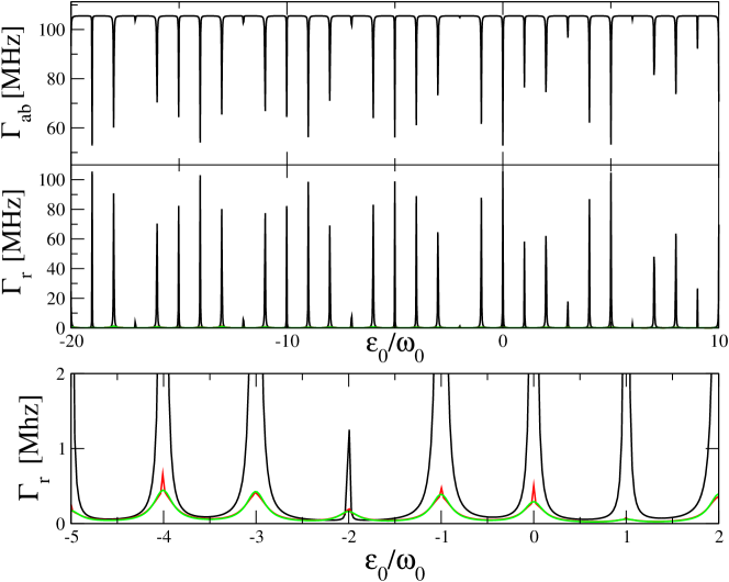
Figure 3: (color online) Upper panel: decoherence rate $\Gamma_{ab}$ obtained in the FM formalism, as a function of the normalized flux detuning $\epsilon_{0}/\omega_{0}$. Intermediate panel: relaxation rate $\Gamma_{r}$ as a function of (normalized) flux detuning obtained within the FM formalism (black solid line). Rate $2W$ obtained from Eq.(6) with $\Gamma_{2}=100$ MHz (green line) and after replacing $\Gamma_{2}\rightarrow\Gamma_{ab}$ (red line). The lower panel shows an enlarge view to stress the differences between $\Gamma_{r}$ and $2W$ close to resonances. Parameters are $\Delta/h=19\,$ MHz, $\omega_{0}/(2\pi)=125\,$ MHz, $A_{1}=3\,m\Phi_{0}$ and $A_{2}=1.65\,m\Phi_{0}$. For the FM calculations the bath is ohmic, $J(\omega)=\gamma\omega$, at temperature $T=20mK$ with coupling $\gamma=0.001$.

Although the resonance condition could seem very sharp to be experimentally fulfilled, significant increments in the values of $\Gamma_{r}$ relative to the background values can be also appreciated in a close vicinity, as it is displayed in Fig.4(a).

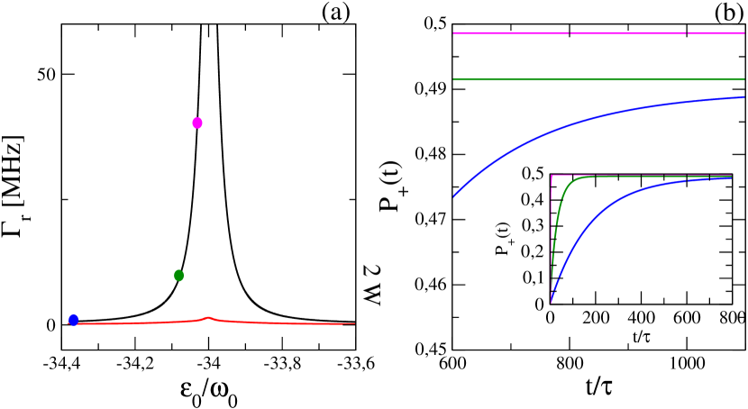
Figure 4: (color online) (a) Relaxation rates rate $\Gamma_{r}$ close to a resonance obtained within the FM formalism as a function of the normalized flux detuning $\epsilon_{0}/\omega_{0}$ and for the same parameters than in Fig.(3). The red curve corresponds to $\Gamma=2W$ obtained from Eq.(6), after replacing $\Gamma_{2}\rightarrow\Gamma_{ab}$. The chosen resonance corresponds to $\epsilon_{0}/\omega_{0}=-34$. (b) Excited state ocupation probability $P_{+}(t)$ as a function of the normalized time $t/\tau$, obtained for three sampled values of $\Gamma_{r}$ (identified by the dots in panel (a)). In each case, the initial state is the ground state of the TLS Hamiltonian Eq.(2) for the correspondent flux detuning $\epsilon_{0}/\omega_{0}$

Relative changes of $\sim 10-20\%$ in $\epsilon_{0}/\omega_{0}$, produce concomitant variations in the values of $\Gamma_{r}$ which give rise to different profiles for the associated excited state occupation probabilities $P_{+}(t)$ (see Fig.4(b)). Even for time scales $t\sim t_{exp}\sim 1000\tau$ appreciable differences still persist in the respective $P_{+}(t_{exp})$.

IV Computing averages and fluctuations in the rates: The mesoscopic analogy

The total accumulated phase during the driving protocol is controlled by the asymmetry parameter $\alpha$, which modifies the biharmonic waveform. As a consequence, $2W$ and $\Gamma_{r}$ should experience, besides the sensitivity on $\epsilon_{0}$, fluctuations as a function of $\alpha$. gustavsson

As we already mentioned, the transition rate induced by the driving, $W$, was identified in Ref.gustavsson, with an effective transition amplitude -the essential ingredient to determine the conductance in the Landauer formalism. datta Under the assumption that the equilibration rate can be written as $\Gamma=2W$, the approach was to associate the fluctuations in $\Gamma$ as function of the dc flux, with the Universal conductance fluctuations (UCF), in analogy with mesoscopic electronic systems.varios_ucf

In the previous section, we have seen that for time scales close to full relaxation and around resonances with the driving field, important and quantitative differences emerge between $2W$ and the relaxation (equilibration) rate, $\Gamma_{r}$, obtained within the FM formalism. Associated with this, the respective fluctuation patterns will also exhibit different behaviours, as we show in the following.

The averages $<2W>$ and $<\Gamma_{r}>$, over $\varepsilon_{0}$, are defined as $\langle...\rangle=\frac{1}{\varepsilon^{max}}\int_{0}^{\varepsilon^{max}}...\,d\varepsilon_{0}\,$, and play the role of ensemble averages over different scatterers configurations. In the case of the phenomenological approach we computed from Eq.(6):

$$\langle W\rangle=\frac{\Delta^{2}}{2\varepsilon^{max}}\sum_{nn^{\prime}mm^{\prime}}\lambda_{nn^{\prime}mm^{\prime}}\cos{((n-n^{\prime})\alpha)}$$ (11)

$$\left[\arctan{\left(\frac{(2m-n)\omega_{0}}{\Gamma_{2}}\right)}-\arctan{\left(\frac{(2m-n)\omega_{0}-\varepsilon^{max}}{\Gamma_{2}}\right)}\right]\;,$$

and

$$\langle W^{2}\rangle=\frac{1}{\varepsilon^{max}}\int_{0}^{\varepsilon^{max}}W^{2}d\varepsilon_{0}\;.$$ (12)

Although $\langle W^{2}\rangle$ does not have a simple analytic expression, its numerical evaluation is straightforward. The fluctuations in $2W$ are defined as $\sigma_{2W}=2\sqrt{\langle W^{2}\rangle-\langle W\rangle^{2}}$

In the case of the relaxation rate $\Gamma_{r}$, its average $\langle\Gamma_{r}\rangle$ and fluctuations $\sigma_{r}$, have been computed numerically.

In Fig.5(a) we plot the averaged rates relative to its values at $\alpha=0.5$, i.e $\langle\Gamma_{r}\rangle_{n}\equiv\langle\Gamma_{r}\rangle/\langle\Gamma_{r}\rangle_{(\alpha=0.5)}$ and $\langle 2W\rangle_{n}\equiv\langle 2W\rangle/\langle 2W\rangle_{(\alpha=0.5)}$, in order to establish a fair comparison for different bath temperatures, couplings $\gamma$ or dephasing rates $\Gamma_{2}$, respectively.

Even after performing the averages in flux detuning, strong fluctuations are still visible as a function of $\alpha$. Notice that $\langle 2W\rangle_{n}$ is almost independent of $\alpha$ and the dephasing rate $\Gamma_{2}$, in agreement with the results of Ref.gustavsson, . On the other hand, $\langle\Gamma_{r}\rangle_{n}$ exhibit a sharp dip at $\alpha=0$, that could be interpreted as the fingerprint of the Weak Localization (WL) correction- in analogy to the correction present in the quantum conductance of mesoscopic disordered systems. varios_wl The relative fluctuations (normalized to the squared mean values) are defined as $\sigma_{r}/\langle\Gamma_{r}\rangle^{2}$ and $\sigma_{2W}/\langle 2W\rangle^{2}$, and are plotted in Fig.5(b). The profiles resembles the UCF found in short mesoscopic wires, with the fluctuations at $\alpha=0$ enhanced compared to the fluctuations for $\alpha\neq 0$, as the theory of UCF predicts when the time revesal symmetry is broken. varios_ucf

The WL correction and the UCF tend to wash out as either the effective temperature and/or the coupling with the environment are increased, as expected when decoherence and relaxation processes become more efficient. This is clearly observed in Figs.5(a) and (b). In addition, the profiles remain almost undisturbed when the product of the effective temperature $T$ times the bath coupling $\gamma$ remains constant, although each one is varied separately. This is consistent with the well known result that the dominant contribution to the decoherence rate depends on the product $\gamma T$. caspar

We want to point out some limitations of the phenomenological approach employed in Sec.III.1 and followed in Ref.gustavsson, . On one hand, it disregards relaxation assuming that the equilibration rate $\Gamma$ is given by $2W$. As a consequence the equilibration rates result largely underestimated close to resonances, as we emphasized when describing Fig.3. On the other hand, the interpretation of $\Gamma$ as a conductance is only well justified away from resonances, when is satisfied that $\Gamma\sim 2W$.

Last but not least, we want to comment on the detection of the WL effect, which has not been measured in Ref.gustavsson, . To our view the limitation which precludes the experimental observation of the WL-like effect is not the driving protocol, as the authors of Ref.gustavsson, suggested, but mainly the difficulty in capturing the extremely sharp resonant conditions as the flux detuning is swept, and also the relatively short experimental decoherence times $T_{2}$. From the theory of disordered electronic systems it is known that the size of the Weak Localization correction scales (logarithmically) with the dephasing time $\tau_{\phi}\propto T_{2}$.varios_wl

Consistent with this result, Fig.5(a) shows very well defined dips in $\langle\Gamma_{r}\rangle_{n}$ at $\alpha=0$, for values of the coupling $\gamma=0.004\sim 0.001$ and temperature of 20 mK-as the reported experimentally. These values give decoherence rates $\Gamma_{2}\sim 25-30$ MHz ($T_{2}=1/\Gamma_{2}\simeq 30-40$ns). Thus it is expected that for slightly larger values of $T_{2}$- but not so far from the reported $T_{2}\sim 10ns$, it could be possible to experimentally access to the full WL dip, once the resonance conditions can be explored.

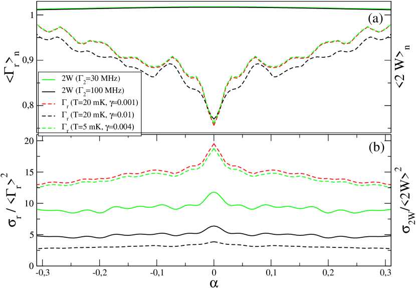
Figure 5: (color online) normalized rates $<\Gamma_{r}>_{n}$ and $<2W>_{n}$ (panel (a)) and normalized standard deviations $\sigma_{r}/<\Gamma_{r}>^{2}$ and $\sigma_{2W}/<2W>^{2}$ (panel (b)) averaged from $-4m\Phi_{0}$ to $0m\Phi_{0}$ as a function of the time reversal broken parameter $\alpha$. The different values of the dephasing rate $\Gamma_{2}$ used to compute $\Gamma=2W$ and the values of the temperature $T$ and bath coupling constant $\gamma$ employed to compute the rates $\Gamma_{r}$ within the FM formalism, are respectively specified in the inset. FQ parameters are $\Delta/h=19\,$ MHz, $\omega_{0}/(2\pi)=125\,$ MHz, $A_{1}=3\,m\Phi_{0}$ and $A_{2}=1.65\,m\Phi_{0}$.

V Conclusions and perspectives

In this work we have tested fluctuation effects associated to broken time reversal symmetry in FQ driven by a biharmonic (dc + ac) magnetic flux with a phase lag.

Employing the full Floquet Markov Master Equation we have computed relaxation $\Gamma_{r}$ and decoherence $\Gamma_{ab}$ rates, both resulting strongly dependent on the phase lag and the dc flux detuning, exhibiting appreciable fluctuations. As a function of the dc flux and away from the resonance conditions with the driving field, $\Gamma_{ab}\rightarrow\Gamma_{2}$ and $\Gamma_{r}\rightarrow\Gamma_{1}$ with $\Gamma_{2}=1/T_{2}>>\Gamma_{1}=1/T_{1}$, i.e. in agreement with the relaxation and decoherence rates predicted for the undriven FQ. However, close to resonances both rates show large variations compared to the respective values out of resonances, even satisfying $2\Gamma_{ab}\sim\Gamma_{r}$.

The relaxation (equilibration) rate $\Gamma_{r}$ can be accessed experimentally by measuring the decay of the FQ excited state population. Recently the fluctuations in the measured equilibration rate have been analized and associated to Universal conductance fluctuations (UCF), following an analogy to well known phenomena exhibited in disordered mesoscopic electronic systems. gustavsson However, as we discuss in extent along this work, the mesoscopic analogy is only well justified for the out of resonance regime, when the equilibration rate can be described in terms of a transition probability induced by the driving protocol.

Besides UCF, we also predict that the Weak Localization effect can be detected for the biharmonic driving protocol. However to observe this effect, the experiments should be performed in a more coherent regime, in which larger values of $T_{2}$ could be attained. Nowadays the control on the environmental bath degrees of freedom is a promising way to enlarge coherence, as have been recently proposed and tested. ferron_prl ; paavola ; chen

By increasing the driving amplitude, more avoided crossings of the FQ can be reached, enabling the computation of averages and fluctuations beyond the weak scattering limit- which in fact is a limitation of the present approach to the mesoscopic analogy. This regime is experimentally attainable as the amplitude spectroscopy experiments bylan2009 have proven.

We acknowledge support from CNEA, UNCuyo (P 06/ C455), CONICET PIP11220150100218, PIP11220150100327 and ANPCyT PICT2011-1537, PICT2014-1382)

References

- (1) S. Datta, Electronic transport in Mesoscopic Systems (Cambridge: Cambridge University Press) (1995).
- (2) A. Benoit et. al., Phys. Rev. Lett. 58 2343, (1986). S. Washburn and R.A. Webb, Rep. Prog. Phys. 55 1311 (1992).
- (3) G. Bergmann, Phys. Rev. B 25 2937 (1982); D. J. Bishop et. al., Phys. Rev. B 26 773 (1982).
- (4) E. Akkermans , G. Montambaux , J. L. Pichard and J. Zinn-Justin, Mesoscopic quantum physics (Amsterdam: Elsevier) (1994).
- (5) T.P.Orlando, L.S. Levitov, L. Tian, C.H. van der Wal and S. Lloyd, Orlando T P et al J.E. Mooij, L. Tian, C.H. van der Wal, L.S. Levitov, S. Lloyd, J.J. Mazo, Phys. Rev. B 60 15398, (1999).
- (6) I. Chiorescu et al, Science 299 1869 2003).
- (7) W. D. Oliver et al, Science 310 1653 (2005).
- (8) J. Q. You and F. Nori, Nature 474 589 (2011).
- (9) A. Ferrón and D. Dominguez, Phys. Rev. B 81, 104505 (2010).
- (10) S. Gustavsson , J. Bylander and W. D. Oliver, Phys. Rev. Lett. 110, 016603 (2013).
- (11) J. Bylander, M. S. Rudner, A. V. Shytov, S. O. Valenzuela, D. M. Berns, K. K. Berggren, L. S. Levitov, and W. D. Oliver, Phys. Rev. B 80, 220506(R) (2009).
- (12) F. Forster, M. Mühlbacher, R. Blattmann, D. Schuh, W. Wegscheider, S. Ludwig, and S. Kohler, Phys. Rev. B 92 245422 (2015).
- (13) A. M. Satanin, M. V. Denisenko, A. I. Gelman, and Franco Nori,Phys. Rev. B 90 104516 (2014).
- (14) R. Blattmann, P. Hänggi, and Sigmund Kohler, Phys. Rev. A 91 042109 (2015).
- (15) D. M. Berns et al, Nature 455 51 (2008); W.D. Oliver and S. O. Valenzuela, Quantum Inf. Process 8 261 (2009).
- (16) A. Ferrón , D. Domínguez and M. J. Sánchez , Phys. Rev. B 82 134522 (2010).
- (17) Y. Nakamura , Y. A. Pashkin and J.S. Tsai, Phys. Rev. Lett. 87 246601 (2001).; M. Sillanpaa et al, Phys. Rev. Lett. 96 187002 (2006).; c.M. Wilson et al, Phys. Rev. Lett. 98 257003 (2007).
- (18) M. Mark et al, Phys. Rev. Lett. 99 113201 (2007).
- (19) P. Huang et al, Phys. Rev. X 1 011003 (2011).
- (20) G. Sun et al Applied Phys. Lett., 94 102502, (2009).
- (21) S. Kohler, T. Dittrich and P. Hänggi, Phys. Rev. E. 55, 300 (1997). S. Kohler, R. Utermann, P. Hänggi, and T. Dittrich, Phys. Rev. E. 58, 7219 (1998).
- (22) A. Ferrón, D. Domínguez and M. J. Sánchez, Phys. Rev. Lett. 82, 134522 (2012).
- (23) A. Ferrón A, D. Domínguez, and M. J. Sánchez, Phys. Rev. B 93, 064521 (2016).
- (24) S. N. Shevchenko ,S. Ashhab and F. Nori, Phys. Rep. 492 1 (2010).
- (25) E. Dupont-Ferrier, B. Roche, B. Voisin, X. Jehl, R. Wac- quez, M. Vinet, M. Sanquer, and S. De Franceschi, Phys. Rev. Lett. 110, 136802 (2013).
- (26) A. Ferrón A, D. Domínguez, and M. J. Sánchez, Journal of Physics: Conference Series 568, 052028 (2014).
- (27) D.M. Berns et al, Phys. Rev. Lett. 97 150502 (2006).
- (28) J. H. Shirley, Phys. Rev. 138, B979 (1965).
- (29) M. Grifoni and P. Hänggi, Phys. Rep. 304, 229 (1998).
- (30) H.-P. Breuer, W. Huber and F. Petruccione, Phys. Rev. E 61, 4883 (2000).
- (31) D. W. Hone, R. Ketzmerick and W. Kohn, Phys. Rev. E 79, 051129 (2009).
- (32) M. C. Goorden, M. Thorwart and M. Grifoni, Phys. Rev. Lett. 93, 267005 (2004); Eur. Phys. J. B 45, 405 (2005).
- (33) J. Hausinger and M. Grifoni, Phys. Rev. A 81, 022117 (2010).
- (34) C. H. van der Wal et al, Eur. Phys. J. B 31, 111 (2003); G. Burkard, R. H. Koch, and D. P. DiVincenzo, Phys. Rev. B 69, 064503 (2004).
- (35) E. Paladino, Y. M Galperin, G. Falci and B. L . Atlshuler, Rev. Mod. Phys. 86, 361 (2014).
- (36) Y. Makhlin, G. Schön, and A. Shnirman, Rev. Mod. Phys. 73, 357 (2001).
- (37) M. H. S. Amin and D. Averin, Phys. Rev. Lett. 100, 197001 (2008);
- (38) S. Gasparineti, P. Solinas, S. Pugnetti, R. Fazio, and J. P. Pekola, Phys. Rev. Lett. 110, 150403 (2013).
- (39) J. Paavola and S. Maniscalco, Phys. Rev. A 82, 012114 (2010).
- (40) Z. Chen, J. Kelly, C. Quintana, R. Barends, B. Campbell, Yu Chen, B. Chiaro, A. Dunsworth, A. G. Fowler, E. Lucero, E. Jeffrey, A. Megrant, J. Mutus, M. Neeley, C. Neill, P. J. J. O’Malley, P. Roushan, D. Sank, A. Vainsencher, J. Wenner, T. C. White, A. N. Korotkov, and John M. Martinis, Phys. Rev. Lett. 116 116, 020501 (2016).