Collapse transition of the interacting prudent walk

Abstract.

This article is dedicated to the study of the 2-dimensional interacting prudent self-avoiding walk (referred to by the acronym IPSAW) and in particular to its collapse transition. The interaction intensity is denoted by $\beta>0$ and the set of trajectories consists of those self-avoiding paths respecting the prudent condition, which means that they do not take a step towards a previously visited lattice site. The IPSAW interpolates between the interacting partially directed self-avoiding walk (IPDSAW) that was analyzed in details in, e.g., Zwanzig and Lauritzen, (1968), Brak et al., (1992), Carmona et al., (2016) and Nguyen and Pétrélis, (2013), and the interacting self-avoiding walk (ISAW) for which the collapse transition was conjectured in Saleur, (1986).

Three main theorems are proven. We show first that IPSAW undergoes a collapse transition at finite temperature and, up to our knowledge, there was so far no proof in the literature of the existence of a collapse transition for a non-directed model built with self-avoiding path. We also prove that the free energy of IPSAW is equal to that of a restricted version of IPSAW, i.e., the interacting two-sided prudent walk. Such free energy is computed by considering only those prudent path with a general north-east orientation. As a by-product of this result we obtain that the exponential growth rate of generic prudent paths equals that of two-sided prudent paths and this answers an open problem raised in e.g., Bousquet-Mélou, (2010) or Dethridge and Guttmann, (2008). Finally we show that, for every $\beta>0$, the free energy of ISAW itself is always larger than $\beta$ and this rules out a possible self-touching saturation of ISAW in its conjectured collapsed phase.

1. Introduction

The collapse transition of self-interacting random walks is a challenging issue, arising in the study of the $\theta$-point of an homopolymer dipped in a repulsive solvent. Different mathematical models have been built by physicists to try and improve their understanding of this phenomenon. For such models, the possible spatial configurations of the polymer are provided by random walk trajectories. In Saleur, (1986), Saleur studies the interacting self-avoiding walk (referred to as ISAW) that is built with self-avoiding paths which are relevant from the physical viewpoint because they fulfill the exclusion volume effect, a feature that real-world polymers indeed satisfy. However, self-avoiding paths, especially in dimension $2$ and $3$, are complicated objects. This is the reason why, in the mathematical literature, collapse transition models were rather built by either relaxing the self-avoiding feature of the paths (see for instance van der Hofstad and A.Klenke, (2001) or van der Hofstad et al., (2002)) or by considering partially directed paths. This is the case for the interacting partially directed self-avoiding walk (referred to as IPDSAW) that was introduced in Zwanzig and Lauritzen, (1968) and subsequently studied in e.g. Brak et al., (1992) or Nguyen and Pétrélis, (2013), Carmona et al., (2016) and Carmona and Pétrélis, (2016)).

In the present paper, we focus on the interacting prudent self-avoiding walk (referred to as IPSAW), a model built with prudent paths, i.e., non-directed self-avoiding paths which can not take a step towards a previously visited lattice site. The IPSAW clearly interpolates between IPDSAW and ISAW since partially directed paths are prudent paths which themselves are self-avoiding paths. An interesting feature of prudent paths is that although they are non-directed and self-avoiding, the prudent condition, especially in dimension 2, imposes some geometric constraints that makes them more tractable than self-avoiding paths themselves. This can be observed in the existing literature dedicated to prudent walks e.g., in Bousquet-Mélou, (2010) or Beffara et al., (2010).

Organization of the paper

In Section 2, we give a rigorous mathematical definition of IPSAW and we state our main results. Section 3 is dedicated to the comparison of our result with the existing literature. We will in particular show how IPSAW can be viewed as a limiting case of the undirected polymer in a poor solvent studied in van der Hofstad and A.Klenke, (2001) and van der Hofstad et al., (2002) and therefore shed some new light on the existence of a conjectured critical curve for this model. In Section 4, we start by increasing the complexity of the partially directed self-avoiding path by introducing the two-sided prudent self-avoiding path. Then, we show how to decompose a generic prudent path into a collection of two-sided paths. Section 5 is dedicated to the proof of Theorem 2.2 that states the existence of a collapse transition for IPSAW at finite temperature. Section 6 provides an algorithm which shows that the free energy of IPSAW coincides with that of North-East interacting prudent self-avoiding walk (referred to as NE-IPSAW), which is a restriction of IPSAW built with a particular type of two-sided paths, i.e., the Nort-East prudent paths. With Section 7, we provide a lower bound on the free energy of ISAW which allows us to compare the nature of the collapse transitions of IPDSAW or IPSAW with that of ISAW. Finally, in Section 8 we prove the existence of the free energy of NE-IPSAW.

2. The interacting prudent self-avoiding walk (IPSAW)

2.1. Description of the models

Let $L\in\mathbb{N}$ be the system size and let $\Omega_{L}^{\texttt{SAW}}$ be the set of $L$-step prudent paths in $\mathbb{Z}^{2}$, i.e.,

$$\Omega_{L}^{\texttt{PSAW}}=\big{\{}w:=(w_{i})_{i=0}^{L}\in(\mathbb{Z}^{2})^{L+1}\colon\, w_{0}=0,\ w_{i+1}-w_{i}\in\{\leftarrow,\rightarrow,\downarrow,\uparrow\},\ 0\leq i\leq L-1,$$

$$w\ \text{satisfies the prudent condition}\big{\}},$$ (2.1)

where the prudent condition for a path $w$ means that it does not take any step in the direction of a lattice site already visited. We also consider a subset of $\Omega_{L}^{\texttt{PSAW}}$ denoted by $\Omega_{L}^{\texttt{NE}}$ containing those $L$-step prudent paths with a general north-east orientation. We postpone the precise definition of $\Omega_{L}^{\texttt{NE}}$ to Section 4.2 because this requires some additional notations but one easily understands what such path look like with Figure 1(b).

At this stage we build two polymer models: the IPSAW for which the set of allowed spatial configurations for the polymer is given by $\Omega_{L}^{\texttt{PSAW}}$ and its North-East counterpart (NE-IPSAW) for which the set of configurations is given by $\Omega_{L}^{\texttt{NE}}$. For both models, each step of the walk is an abstract monomer and we want to take into account the repulsion between monomers and the environment around them. This is achieved indirectly, by encouraging monomers to attract each other, i.e., by assigning an energetic reward $\beta\geq 0$ to any pair of non-consecutive steps of the walk though adjacent on the lattice $\mathbb{Z}^{2}$. To that aim, we associate with every path $w$ the sequence of those points in the middle of each step, i.e., $u_{i}=w_{i-1}+\frac{w_{i}-w_{i-1}}{2}$ ($1\leq i\leq L$) and we reward every non-consecutive pair $(u_{i},u_{j})$ at distance one, i.e, $\|u_{i}-u_{j}\|=1$, see Figure 1. The energy associated with a given $w\in\Omega_{L}$ is defined by an explicit Hamiltonian, that is

$$\mathrm{H}\,(w):=\sum_{\begin{subarray}{c}i,j=0\\ i<j\end{subarray}}^{L}\mathds{1}_{\{\lVert u_{i}-u_{j}\rVert=1\}},$$ (2.2)

so that $\mathrm{Z}_{\beta,L}$ the partition function of IPSAW and $\mathrm{Z}^{\texttt{NE}}_{\beta,\,L}$ the partition function of the North-east model equal

$$\mathrm{Z}_{\beta,\,L}:=\sum_{w\in\Omega_{L}^{\texttt{PSAW}}}e^{\,\beta\,\mathrm{H}\,(w)}\quad\text{and}\quad\mathrm{Z}^{\texttt{NE}}_{\beta,\,L}:=\sum_{w\in\Omega_{L}^{\texttt{NE}}}e^{\,\beta\,\mathrm{H}\,(w)}.$$ (2.3)

The key objects of our analysis are the free energies of both models, i.e., $\mathrm{F}(\beta)$ and $\mathrm{F}^{\texttt{NE}}(\beta)$ which record the exponential growth rate of the partition function sequences $(\mathrm{Z}_{\beta,\,L})_{L\in\mathbb{N}}$ and $(\mathrm{Z}^{\texttt{NE}}_{\beta,\,L})_{L\in\mathbb{N}}$, respectively. Thus,

$$\mathrm{F}(\beta):=\lim_{L\to\infty}\frac{1}{L}\log\mathrm{Z}_{\beta,\,L}\quad\text{and}\quad\mathrm{F}^{\texttt{NE}}(\beta):=\lim_{L\to\infty}\frac{1}{L}\log\mathrm{Z}^{\texttt{NE}}_{\beta,\,L}.$$ (2.4)

The convergence in the right hand side of (2.4) will be proven in Section 8. The convergence in the l.h.s. of (2.4) is more complicated and it will be obtained as a by-product of Theorem 2.1 below.

2.2. Main results

In the present Section we state our main results and we give some hints about their proof. We pursue the discussion in Section 3 below, by explaining how our results answer some open problems leading to a better comprehension of interacting self-avoiding walk.

With Theorem 2.1 below, we state that the free energies of IPSAW and of NE-IPSAW are equal. Our proof is displayed in Section 6 and is purely combinatorial. It consists in building a sequence of path transformations $(M_{L})_{L\in\mathbb{N}}$ such that for every $L\in\mathbb{N}$, $M_{L}$ maps any generic path in $\Omega_{L}^{\texttt{PSAW}}$ onto a 2-sided prudent path in $\Omega_{L}^{\texttt{NE}}$ and satisfies the following properties:

• for every $w\in\Omega_{L}^{\texttt{PSAW}}$, the difference between the Hamiltonians of $w$ and of $M_{L}(w)$ is $o(L)$,

• the number of ancestors of a given path in $\Omega_{L}^{\texttt{NE}}$ by $M_{L}$ can be shown to be $e^{o(L)}$.

Such a mapping allows us to prove the following theorem.

Theorem 2.1.

For $\beta\geq 0$,

$$\mathrm{F}(\beta)=\mathrm{F}^{\rm\texttt{NE}}(\beta).$$ (2.5)

The free energy equality in (2.5) will subsequently be used to establish Theorem 2.2 below, which states that IPSAW undergoes a collapse transition at finite temperature.

Theorem 2.2.

There exists a $\beta_{c}^{\texttt{IPSAW}}\in(0,\infty)$ such that

$$\mathrm{F}(\beta) >\beta\quad\text{for every}\quad\beta<\beta_{c}^{\texttt{IPSAW}},$$ (2.6)

$$\mathrm{F}(\beta) =\beta\quad\text{for every}\quad\beta\geq\beta_{c}^{\texttt{IPSAW}}.$$

Thus, the phase diagram $[0,\infty)$ is partitioned into a collapsed phase, $\mathcal{C}:=[\beta_{c}^{\texttt{IPSAW}},\infty)$ inside which the free energy (2.4) is linear and an extended phase, $\mathcal{E}=[0,\beta_{c}^{\texttt{IPSAW}})$.

The proof of Theorem 2.2 is displayed in Section 5. It requires to exhibit a loss of analyticity of $\beta\mapsto\mathrm{F}(\beta)$ at some positive value of $\beta$ (which is subsequently denoted by $\beta_{c}^{\texttt{IPSAW}})$. The nature of the proof is much more probabilistic than that of Theorem 2.1. It indeed relies, on the one hand, on the random walk representation of the partially directed version of our model displayed initially in Nguyen and Pétrélis, (2013) and, on the other hand, on the fact that prudent path can be naturally decomposed into shorter partially directed paths.

Since a partially directed self-avoiding path is in particular a generic prudent path, we can compare the critical point of IPSAW with the critical point of IPDSAW, which was computed explicitly in e.g. Brak et al., (1992); Nguyen and Pétrélis, (2013). We obtain that

$$\beta_{c}^{\texttt{IPDSAW}}\,\leq\,\beta_{c}^{\texttt{IPSAW}}.$$ (2.7)

The inequality in (2.7) is somehow not satisfactory since one wonders whether it is strict or not. This issue is left as an open question and will be discussed further in Section 3.3.

We conclude this section by considering the $2$-dimensional Interacting Self-Avoiding Walk (ISAW) defined exactly like the IPSAW in (2.2) but with a larger set of allowed configurations, that is (in size $L\in\mathbb{N}$)

$$\Omega_{L}^{\texttt{SAW}}:=\big{\{}w:=(w_{i})_{i=0}^{L}\in(\mathbb{Z}^{2})^{L+1}\colon\, w_{0}=0,\ w_{i+1}-w_{i}\in\{\leftarrow,\rightarrow,\downarrow,\uparrow\},\ 0\leq i\leq L-1,$$ (2.8)

$$w\ \text{satisfies the self-avoiding condition}\big{\}}.$$

We denote by $Z_{L,\beta}^{\texttt{ISAW}}$ the partition function of ISAW and we define its free energy as

$$F^{\texttt{ISAW}}(\beta):=\liminf_{L\to\infty}\frac{1}{L}\log Z_{L,\beta}^{\texttt{ISAW}},$$ (2.9)

where the $\liminf$ in (2.9) is chosen to overstep the fact that the convergence of the free energy remains an open issue.

Theorem 2.3.

$$\mathrm{F}^{\texttt{ISAW}}(\beta) >\beta,\quad\text{for every}\quad\beta\in[0,\infty).$$ (2.10)

A straightforward consequence of Theorem 2.3 is that the conjectured collapse transition displayed by ISAW at some $\beta_{c}^{\texttt{ISAW}}$ does not correspond to a self-touching saturation as it is the case for IPDSAW and IPSAW.

3. Discussion

3.1. Background

The ISAW has triggered quite a lot of attention from both the physical and the mathematical communities. Much efforts have been put, for instance, to estimate numerically the value of the critical point $\beta_{c}^{\texttt{ISAW}}$ (see e.g. Tesi et al., 1996a or Tesi et al., 1996b in dimension $3$) or to compute the typical end to end distance of a path at criticality (see e.g. Saleur, (1986)). However, only very few rigorous mathematical results have been obtained about it so far. For example, the existence of a collapse transition is conjectured only and if such transition turns out to occur, obtaining some quantitative results about the geometric conformation adopted by the path inside each phase is even more challenging. In view of the mathematical complexity of ISAW, other models have been introduced, somehow simpler than ISAW and therefore more tractable mathematically.

The first attempt to investigate a simplified version of ISAW is due to Zwanzig and Lauritzen, (1968) with the Interacting Partially Directed Self-Avoiding Walk (IPDSAW). Again the model is defined as in (2.2), but with a restricted set of configurations, i.e.,

$$\Omega_{L}^{\texttt{PDSAW}}:=\big{\{}w:=(w_{i})_{i=0}^{L}\in(\mathbb{N}\times\mathbb{Z})^{L+1}\colon\, w_{0}=0,\ w_{i+1}-w_{i}\in\{\rightarrow,\downarrow,\uparrow\},\ 0\leq i\leq L-1,$$ (3.1)

$$w\ \text{satisfies the self-avoiding condition}\big{\}}.$$

The IPDSAW was first investigated with combinatorial methods in e.g., Brak et al., (1992) where the critical temperature, $\beta_{c}^{\texttt{IPDSAW}}$, is computed. Subsequently, in Nguyen and Pétrélis, (2013) and Carmona et al., (2016) and Carmona and Pétrélis, (2016) a probabilistic approach allowed for a rather complete quantitative description of the scaling limits displayed by IPDSAW in each three regimes (extended, critical and collapsed).

Another simplification of ISAW gave birth to the Interacting Weakly Self-Avoiding Walk (IWSAW), which is built by relaxing the self-avoiding condition imposed in ISAW such that the set of configurations $\Omega_{L}$ contains every $L$-step trajectory of a discrete time simple random walk on $\mathbb{Z}^{d}$ ($d\geq 1$). The Hamiltonian associated with every path rewards the self-touchings and penalizes the self-intersections, i.e, for every $w\in\Omega_{L}$,

$$H\,(w)=-\gamma\sum_{0\leq i<j\leq L}\mathds{1}_{\{w_{i}-w_{j}=0\}}\ +\beta\sum_{0\leq i<j\leq L}\mathds{1}_{\{|u_{i}-u_{j}|=1\}}.$$ (3.2)

Thus, $\gamma\geq 0$ is a parameter that can be tuned to approach the ISAW through the IWSAW, since in the limit $\gamma=\infty$ both models coincide. The IWSAW is investigated in two papers, i.e., van der Hofstad and A.Klenke, (2001) and van der Hofstad et al., (2002) whose results are reviewed in (den Hollander,, 2009, Section 6.1). In van der Hofstad et al., (2002), the existence of a critical curve $\gamma=2d\beta$ between a localized phase and a collapsed phase (also referred to as minimally extended) is proven in every dimension $d\geq 1$. Inside the localized phase (i.e., for $\beta>\gamma/2d$) and with probability arbitrarily close to $1$ the polymer is confined inside a squared box of finite size. Inside the collapsed phase in turn, the typical diameter of the polymer is proven to be at least $L^{1/d}$. It is conjectured that at criticality ($\beta=2d\gamma$), the polymer scales as $L^{1/d+1}$. This is made rigorous in van der Hofstad et al., (2002) when $d=1$. In dimension $d\geq 2$, IWSAW is conjectured to undergo another critical curve $\gamma\mapsto\beta(\gamma)$ between the previously mentioned collapsed phase and an extended phase inside which the typical extension of the path is expected to be that of the self-avoiding walk. This critical curve is expected to have an horizontal asymptote $\beta=\beta^{*}\in(0,\infty)$ and $\beta^{*}$ is itself expected to equal $\beta_{c}^{\texttt{ISAW}}$.

3.2. Discussion of the results

As mentioned above, one of the interest of IPSAW is that it interpolates between IPDSAW, which is now very well understood, and ISAW (or IWSAW at $\gamma=\infty$) about which most theoretical issues remain open. From this perspective, Theorem 2.2 clearly constitutes a step forward in the investigation of ISAW since, up to our knowledge, IPSAW is the first non-directed model of interacting self-avoiding walk for which the existence of a collapse transition is proven rigorously.

At first sight, Theorem 2.1 may appear as an intermediate step in the proof of theorem 2.2. The fact that the free energies of IPSAW and of NE-IPSAW are equal allows us to prove Theorem 2.2 with $2$-sided prudent paths only. However, the importance of Theorem 2.1 goes beyond IPSAW itself. The 2-sided prudent trajectories have indeed been studied already in the mathematical litterature, see e.g., Bousquet-Mélou, (2010), Dethridge and Guttmann, (2008) or Beaton and Iliev, (2015). It was conjectured in Bousquet-Mélou, (2010) or Dethridge and Guttmann, (2008) that the exponential growth rate of the cardinality of $2$-sided prudent paths (as a function of their length) equals that of generic prudent paths and this is precisely what Theorem 2.1 says at $\beta=0$. Moreover this result supports somehow the conjecture that the scaling limit of the uniform prudent walk should be the same as that of its $2$-sided counterpart, see Bousquet-Mélou, (2010). We discuss this conjecture in Section 3.3 below.

As mentioned below Theorem 2.3, the fact that ISAW does not give rise to a self-touching saturation when $\beta$ becomes large enough indicates that the nature of its phase transition differs from that of IPDSAW and IPSAW. Theorem 2.3 tells us that for every $\beta>0$, one can display a subset of trajectories whose contribution to the free energy is strictly larger than $\beta$. As a consequence, there is no straightforward inequality between the conjectured critical point $\beta_{c}^{\text{ISAW}}$ and $\beta_{c}^{\text{IPDSAW}}$ or between $\beta_{c}^{\text{ISAW}}$ and $\beta_{c}^{\text{IPSAW}}$.

3.3. Open problems

We state 3 open problems which, in our opinion, are interesting but require to bring the instigation of IPSAW and ISAW some steps further. We discuss those 3 issues subsequently.

1. Compute $\beta_{c}^{\texttt{IPSAW}}$ and therefore determine whether or not $\beta_{c}^{\texttt{IPSAW}}>\beta_{c}^{\texttt{IPDSAW}}$.

2. Provide the scaling limit of IPSAW in its three regimes, i.e., extended, critical and collapsed.

3. Prove that ISAW also undergoes a collapse transition at some $\beta>0$.

Concerning the first open question above, one should keep in mind Theorem 2.1. Proving that $\beta_{c}^{\texttt{IPSAW}}>\beta_{c}^{\texttt{IPDSAW}}$ indeed requires to check that $\mathrm{F}^{\texttt{NE}}(\beta_{c}^{\texttt{IPDSAW}})>\beta_{c}^{\texttt{IPDSAW}}$. For simplicity we set $\beta_{c}=\beta_{c}^{\texttt{IPDSAW}}$. We recall the grand canonical characterization of the free energy, i.e.,

$$\mathrm{F}^{\texttt{NE}}(\beta_{c})-\beta_{c}=\inf\bigg{\{}\gamma>0\colon\;\sum_{L\geq 1}Z_{L,\beta_{c}}^{\texttt{NE}}e^{-(\beta_{c}+\gamma)L}<\infty\bigg{\}}$$ (3.3)

and we observe that a generic NE-prudent path is a concatenation of partially directed path (see (4.3)) satisfying an additional geometric constraint called exit-condition (see Definition 4.3). If we denote by $Z_{L,\beta_{c}}^{\texttt{IPDSAW}}(*)$ the partition function of IPDSAW restricted to those configurations respecting the exit-condition and if we forget about the interactions between the partially directed subpaths constituting a NE-prudent path, we deduce that the inequality

$$\sum_{L\geq 4}Z_{L,\beta_{c}}^{\texttt{IPDSAW}}(*)\,e^{-\beta_{c}L}>1$$ (3.4)

would be sufficient to claim that the l.h.s. in (3.3) is positive. Without the exit condition, i.e., with $Z_{L,\beta_{c}}^{\texttt{IPDSAW}}$ instead of its restricted counterpart, the inequality (3.4) is true. This is a consequence of the random walk representation of IPDSAW displayed in Nguyen and Pétrélis, (2013) which gives that $\sum_{L\geq 4}Z_{L,\beta_{c}}^{\texttt{IPDSAW}}\,e^{-\beta_{c}L}=\infty$ because it equals the expected number of visits at the origin of a recurrent random walk on $\mathbb{Z}$. However, the exit condition imposed to every partially directed subpath constituting a NE-prudent path induces a strong loss of entropy and this is why we are not able to show that (3.4) also holds true.

The second open question would complete the scaling limit of the prudent walk (at $\beta=0$). This problem has been investigated with combinatorial technics in, e.g. (Bousquet-Mélou,, 2010, Proposition 8) for the 3-sided prudent walk. In this case the scaling limit is a straight line along the diagonal and it is conjectured that also the generic prudent walk displays the same scaling limit. With probabilistic tools, the scaling limit of the (kinetic) prudent walk was explored in Beffara et al., (2010). We refer to Beffara et al., (2010) for the precise definition of the kinetic prudent walk, but let us emphasize that its scaling limit is described by an explicit non trivial continuous process, cf. (Beffara et al.,, 2010, Theorem 1).

We may assume that inside its extended phase the scaling limit of IPSAW remains very similar to that of the prudent walk (at $\beta=0$). From this perspective, it would be interesting to get a better understanding of the geometry of IPSAW inside its collapsed phase as well. Since $F(\beta)=\beta$ when $\beta\geq\beta_{c}^{\text{IPSAW}}$, we can state that the fraction of self-touching of a typical path is $1+o(1)$. However, there are various type of paths achieving this condition, e.g., the collapsed configurations of IPDSAW (see (Carmona et al.,, 2016, Section 4)) or configurations filling a square box by turning around their range, and it is not clear at this stage which subclass would contribute the most to the partition function.

The third open question is the most difficult. The fact that one can not display a subset of parameters in $[0,\infty)$ inside which the free energy of ISAW becomes linear illustrates this difficulty.

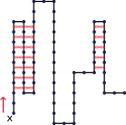
(a) IPDSAW

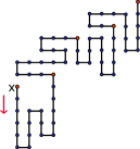
(b) NE-IPSAW

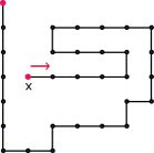
(c) IPSAW

Figure 1. Examples of a PDSAW (A), NE-PSAW (B) and PSAW (C) path. Any path starts at $x$ and its orientation is given by the arrow.
In (A) we have drawn an IPDSAW path made of $11$ stretches: $\ell_{1}=9,\,\ell_{2}=-7,\,\ell_{3}=9,\,\ell_{4}=0,\,\ell_{5}=-12,\,\ell_{6}=0,\,\ell_{7}=5,\,\ell_{8}=0,\,\ell_{9}=5,\,\ell_{10}=-7,\ell_{11}=0$. That path performs $19$ self-touching (drawn in red).

4. Decomposition of a generic prudent path

In this section we describe the different type of path that we will have to take into account in the paper. By order of increasing complexity, we will first introduce in Section 4.1 the partially directed self-avoiding paths and their counterparts satisfying the so called exit condition which is an additional geometric constraints allowing for their concatenation. In section 4.2, we concatenate such partially directed paths to build the two-sided prudent paths. Those two sided path have $4$ possible general orientations; north-east (NE), north-west (NW), south-east (SE) and south-west (SW). Finally in Section 4.3, we will introduce the generic prudent path and observe that each such path can be decomposed in a unique manner into a succession of macro-blocks that are particle case of two-sided prudent paths obeying some additional constraints given by the prudent condition to make possible their concatenation.

We need to define $\oplus$ a concatenation operator on prudent path. We pick $r\in\mathbb{N}$ and we consider $r$ prudent paths denoted by $w_{1},\dots,w_{r}$. We let $w_{1}\oplus w_{2}\oplus\dots\oplus w_{r}$ be the path obtained by attaching the last step of $w_{i-1}$ with the first step of $w_{i}$ for every $2\leq i\leq r$. Then, the sequence $(w_{1},\dots,w_{r})$ is said to be concatenable if $w_{1}\oplus\dots\oplus w_{r}$ itself is a prudent path. Finally, we extend the notation $\oplus$ to the concatenation of sets of prudent path. Therefore, if $(\mathcal{A}_{i})_{i=1}^{r}$ are $r$ sets of paths such that any sequence in $\mathcal{A}_{1}\times\dots\times\mathcal{A}_{r}$ is concatenable, then $\mathcal{A}_{1}\oplus\dots\oplus\mathcal{A}_{r}$ contains all paths obtained by concatenating sequences in $\mathcal{A}_{1}\times\dots\times\mathcal{A}_{r}$.

4.1. Partially directed self-avoiding walk (PDSAW)

The partially directed self-avoiding walk is a random walk on $\mathbb{Z}^{2}$ whose increments are unitary and can take only three possible directions. For instance, when the increments of the path are chosen in $\{\uparrow,\,\downarrow,\,\rightarrow\}$, then the path is west-east oriented. By rotating an west-east path by $\pi/2$ radians we obtain a south-north path, whose increments are chosen in $\{\uparrow,\,\leftarrow,\,\rightarrow\}$, see Figure 2 for two examples of such paths. By repeating twice this rotation, we recover the east-west and the north-south paths. In what follows and for $L\in\mathbb{N}$, the set of west-east partially directed paths of length $L$ (south-north, east-west, north-south respectively) will be denoted by $\Omega_{L,pd}^{\rightarrow}$ ($\Omega_{L,pd}^{\uparrow}$, $\Omega_{L,pd}^{\leftarrow}$, $\Omega_{L,pd}^{\downarrow}$ respectively).

Definition 4.1 (Inter-stretch).

We call inter-stretch every increment in the direction which gives the orientation of a given partially directed path. Therefore, any partially directed path of finite length can be partitioned into $(N-1)$-inter-stretches and $N$-stretches, $(\ell_{1},\dots,\ell_{N})\in\mathbb{Z}^{N}$, for some $N\in\mathbb{N}$. For $i\in\{1,\dots,N\}$, the modulus of $\ell_{i}$ gives the number of unitary steps composing the $i$-th stretch and when $\ell_{i}\neq 0$, the sign of $\ell_{i}$ gives its orientation. In a west-east or east-west path, we say that $\ell_{i}$ has a south-north orientation ($\uparrow$) if $\ell_{i}>0$ and north-south ($\downarrow$) if $\ell_{i}<0$. In a south-north or north-south path, we say that $\ell_{i}$ has an west-east orientation ($\rightarrow$) if $\ell_{i}>0$ and east-west ($\leftarrow$) if $\ell_{i}<0$ (see Figure 2). Thus, e.g.,

$$\Omega_{L,pd}^{\to}=\bigcup_{N=1}^{L}\Big{\{}\ell=(\ell_{i})_{i=1}^{N}\in\mathbb{Z}^{N}\colon\,N-1+|\ell_{1}|+\dots+|\ell_{N}|=L\Big{\}}.$$

Remark 4.2.

In this paper we also take into account those partially directed path with only one vertical stretch and zero inter-stretches (thus $N=1$ in Definition 4.1). This is a slight difference with respect to Carmona et al., (2016)), in which $N\geq 2$.

In Section 4.2 we define the two-sided path. They are obtained by concatenating alternatively, e.g., some west-east partially directed paths with some south-north partially directed paths. However, concatenating such oriented path requires an additional geometric constraint called exit-condition which requires a proper definition.

Definition 4.3 (Exit condition).

Let $N\in\mathbb{N}$ and let $\ell=(\ell_{1},\dots,\ell_{N})\in\mathbb{Z}^{N}$ be an arbitrary sequence of stretches. Then, $\ell$ satisfies the upper exit condition if its last stretch finishes strictly above all other stretches, i.e.,

$$\ell_{1}+\cdots+\ell_{N}\,>\,\max_{0\leq i<N}\{\ell_{1}+\cdots+\ell_{i}\},$$

and $\ell$ satisfies the lower exit condition or if its last stretch finishes strictly below all other stretches, i.e.,

$$\ell_{1}+\cdots+\ell_{N}\,<\,\min_{0\leq i<N}\{\ell_{1}+\cdots+\ell_{i}\}.$$

Definition 4.4 (Oriented blocks).

An arbitrary west-east partially directed path $(\ell_{1},\ell_{2},\dots,\ell_{N})$ is called upper oriented if its first stretch is negative and if it obeys the upper exit condition (see Figure 2 (A)). Otherwise, it is called lower oriented if its first stretch is positive and if it obeys the lower exit condition. We denote by $\mathcal{O}_{L}^{\to,+}$ the set of upper west-east oriented blocks of size $L$ and by and by $\mathcal{O}_{L}^{\to,-}$ the set of lower west-east oriented blocks, i.e.,

$$\mathcal{O}_{L}^{\to,+} :=\{\ell\in\Omega_{L,pd}^{\to}\colon\ell_{1}<0\ \text{and $\ell$ satisfies the \emph{upper exit condition}}\},$$ (4.1)

$$\mathcal{O}_{L}^{\to,-} :=\{\ell\in\Omega_{L,pd}^{\to}\colon\ell_{1}>0\ \text{and $\ell$ satisfies the \emph{lower exit condition}}\}.$$ (4.2)

We define analogously the sets $\mathcal{O}_{L}^{\uparrow,+}$ and $\mathcal{O}_{L}^{\uparrow,-}$ of upper south-north oriented blocks and of lower south north oriented blocks, respectively, and so on.

We stress that for satisfying the exit condition it must hold that $N\geq 2$, i.e., we need at least two stretches.

4.2. Two-sided prudent path

With the oriented blocks (recall definition 4.4) in hand, we can define a larger class of prudent paths: the 2-sided prudent paths, which ultimately will constitute the building bricks of the prudent path. Those $2$-sided prudent path have a general orientation that can be north-east (NE), north-west (NW), south-west (SW) or south-east (SE). In the rest of the section we focus on NE-prudent path, but all definitions we give can easily be adapted to consider a generic oriented (NE, NW, SE, SW) prudent self-avoiding path.

As mentioned above, north-east prudent path are obtained by considering a family of west-east oriented blocks and a family of south-north oriented blocks and by concatenating them alternatively.

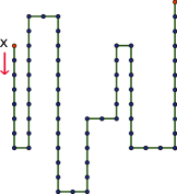
(a) A west-east block.

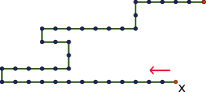
(b) A south-north block.

Figure 2. The west-east oriented block (A) is made of $12$ stretches and is upper oriented since $\ell_{1}<0$ and $\ell_{1}+\dots+\ell_{12}>\displaystyle\max_{1\leq i\leq 11}\{\ell_{1}+\dots+\ell_{i}\}$.
Analogously, the south-north block (B) is upper oriented as well.

Definition 4.5 (NE-prudent path).

To define a NE-prudent self-avoiding path of length $L\in\mathbb{N}$ we consider $r\in\mathbb{N}$ oriented blocks, $(\pi_{1},\dots,\pi_{r})$, of length $t_{1},\dots,t_{r}$ respectively, with $t_{1}+\cdots+t_{r}=L$ and $t_{i}\geq 4$. We assume that those blocks indexed by odd integers are either all upper west-east oriented (in which case all blocks indexed by even integers are upper south-north oriented) or all upper south-north oriented (in which case all blocks indexed by even integers are upper west-east oriented). In definition 4.4 we have imposed that an upper oriented block starts with a negative stretch but this constraint can be relaxed for $\pi_{1}$ (the first oriented block of the sequence). We have also imposed that an upper oriented block satisfies the upper exit condition but this constrain can be relaxed for $\pi_{r}$ (the last block of the sequence). See Figure 3 for an example of a NE-prudent path with these $2$ constraints relaxed. Then, we concatenate $\pi_{1},\dots,\pi_{r}$ (which is possible because the first $r-1$ blocks satisfy the exit condition) and the resulting path is denoted by $\pi_{1}\oplus\dots\oplus\pi_{r}$. We call such path a NE-prudent self-avoiding path, see Figure 3. The sequence $(\pi_{1},\dots,\pi_{r})$ is called the block decomposition of the path and it is unique.

We now provide a formal definition of $\Omega_{L}^{\texttt{NE}}$:

$$\Omega_{L}^{\texttt{NE}}= \bigcup_{r\in 2\mathbb{N}}\bigcup_{t_{1}+\dots+t_{r}=L}\big{[}\mathcal{O}_{t_{1},*}^{\to,+}\oplus\mathcal{O}_{t_{2}}^{\uparrow,+}\oplus\dots\oplus\mathcal{O}_{t_{r-1}}^{\to,+}\oplus\mathcal{O}_{t_{r},\square}^{\uparrow,+}\Big{]}\cup\Big{[}\mathcal{O}_{t_{1},*}^{\uparrow,+}\oplus\mathcal{O}_{t_{2}}^{\to,+}\oplus\dots\oplus\mathcal{O}_{t_{r-1}}^{\uparrow,+}\oplus\mathcal{O}_{t_{r},\square}^{\to,+}\Big{]}$$ (4.3)

$$\cup\ \bigcup_{r\in 2\mathbb{N}-1}\bigcup_{t_{1}+\dots+t_{r}=L}\big{[}\mathcal{O}_{t_{1},*}^{\to,+}\oplus\mathcal{O}_{t_{2}}^{\uparrow,+}\oplus\dots\oplus\mathcal{O}_{t_{r-1}}^{\uparrow,+}\oplus\mathcal{O}_{t_{r},\square}^{\to,+}\Big{]}\cup\Big{[}\mathcal{O}_{t_{1},*}^{\uparrow,+}\oplus\mathcal{O}_{t_{2}}^{\to,+}\oplus\dots\oplus\mathcal{O}_{t_{r-1}}^{\to,+}\oplus\mathcal{O}_{t_{r},\square}^{\uparrow,+}\Big{]},$$

where the notations $\mathcal{O}_{t,*}^{\,\cdot\,,+}$ means that the condition $\ell_{1}<0$ has been removed from (4.1) and $\mathcal{O}_{t,\square}^{\,\cdot\,,+}$ means that the exit condition has been removed from (4.1).

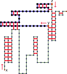
Figure 3. A NE-PSAW path made of three blocks: the first and the third blocks are west-east (in green) and the second block is south-north (in blue). The first block starts at $x$, the second block starts at $y$ and the third block starts at $z$. Their orientation is given by the arrow. Interactions in each block and between different blocks are highlighted in red.

Remark 4.6.

Let us observe that indeed $\Omega_{L,pd}^{\to}$ and $\Omega_{L,pd}^{\uparrow}$ are NE-prudent self-avoiding walk. It corresponds to the case in which we have only one block, i.e., $r=1$.

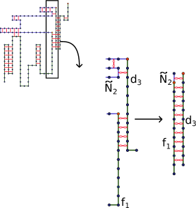
Figure 4. On the left, a NE-PSAW path made of three blocks. In the picture we zoom in on the interactions between the third block and the rest of path. We recall that the third block can only interact with its two preceding blocks, i.e., the first and the second one. We call $f_{1}$ the last vertical stretch of the first block and $d_{3}$ the first vertical stretch of the third block. The interactions between the first and the third blocks involve $f_{1}$ and $d_{3}$ while the interactions between the second and the third blocks involve $d_{3}$ and $\tilde{N}_{2}$ (the number of inter-stretches in the second block that may truly interact with $d_{3}$, on the picture $\tilde{N}_{2}=1$). Such interactions are bounded above by $(\tilde{N}_{2}+f_{1})\,\tilde{\wedge}\,d_{3}$.

4.3. Interacting prudent self-avoiding walk

In this section we show how a general prudent path can be decomposed in a unique manner into a sequence of 2-sided prudent paths called macro-blocks. There is a difference between the decomposition of a two-sided path into oriented blocks and that of a generic prudent path into macro-blocks. We have indeed seen in Section 4.5 above that the exit condition, which is an intrinsic constraint, was sufficient to make sure that oriented blocks alternatively west-east and south-north are concatenable. However, to make sure that a given family of 2-sided prudent paths is concatenable, one can not rely on some intrinsic geometric constraint anymore. Such a family must indeed satisfy a global constraint, that is, each 2-sided prudent path has to satisfy the prudent condition with the all path it will be attached to and this condition is not intrinsic anymore, see Figure 5.

We recall that a walk is said to be prudent if none of its steps point in the direction of its range. In the sequel we refer to this constraint as the prudent condition.

4.3.1. Macro-block decomposition

Let us start by noticing that a prudent walk can be viewed as a sequence of NE, NW, SE, SW two-sided sub-paths that we will call macro-block, see Figure 5.

Definition 4.7.

For very $m,L\in\mathbb{N}$ we denote by $\Theta_{m,L}$ the set gathering all concatenable sequences of $m$ two-sided paths such that the cumulated length of the two-sided paths in the sequence is $L$ and such that:

1. two consecutive two-sided paths in the sequence do not have the same orientation,

2. the first $m-1$ two-sided paths in the sequence contain at least $2$ oriented blocks.

For the ease of notation, we recall (4.3) and we let $\Omega_{L,\triangle}^{\texttt{NE}}$ be the set of north-east prudent path containing at least two oriented blocks (the same definition holds with the $3$ others possible orientations of a two-sided path). Thus,

$$\Theta_{m,L}=\bigcup_{t_{1}+\dots+t_{m}=L}\ \bigcup_{\begin{subarray}{c}(x_{i})_{i=1}^{m}\in\{\texttt{NE},\texttt{NW},\texttt{SE},\texttt{SW}\}\\ x_{i-1}\neq x_{i},\ i\leq r\end{subarray}}\begin{aligned} \Big{\{}(\Lambda_{1},\dots,\Lambda_{m})\in\,\Omega_{t_{1},\triangle}^{x_{1}}\times\dots&\times\Omega_{t_{m-1},\triangle}^{x_{m-1}}\times\Omega_{t_{m}}^{x_{m}}\colon\\ &(\Lambda_{1},\dots,\Lambda_{m})\ \text{is concatenable}\,\Big{\}}\end{aligned}$$ (4.4)

Finally, we observe that any prudent path of length $L$ can be decomposed into a sequence of macro-blocks in $\cup_{m\geq 1}\Theta_{m,L}$ and moreover, thanks to the conditions (1) and (2) in Definition 4.7 we can assert that such decomposition is unique. Therefore, we may partition $\Omega_{L}^{\texttt{PSAW}}$ as

$$\Omega_{L}^{\texttt{PSAW}}=\cup_{m\geq 1}\{\Lambda_{1}\oplus\dots\oplus\Lambda_{m}\colon(\Lambda_{1},\dots,\Lambda_{m})\in\Theta_{m,L}\}$$ (4.5)

An example of such decomposition is provided in Figure 5.

4.3.2. Upper bound on the number of macro-block in the decomposition of a generic prudent path.

The prudent condition imposes strong constraints on the number of macro-block composing the path: if we consider the smallest rectangle embedding the whole path, then whenever the random walk wants to start a new macro-block, it must cross the whole rectangle in one direction and in such direction the length of the rectangle is increased by at least one unit. Therefore the longer it is the path, the harder (expensive) it becomes to start a new macro-block. In Lemma 4.8 we provide an upper bound on the number of macro-blocks in a prudent path of a given length.

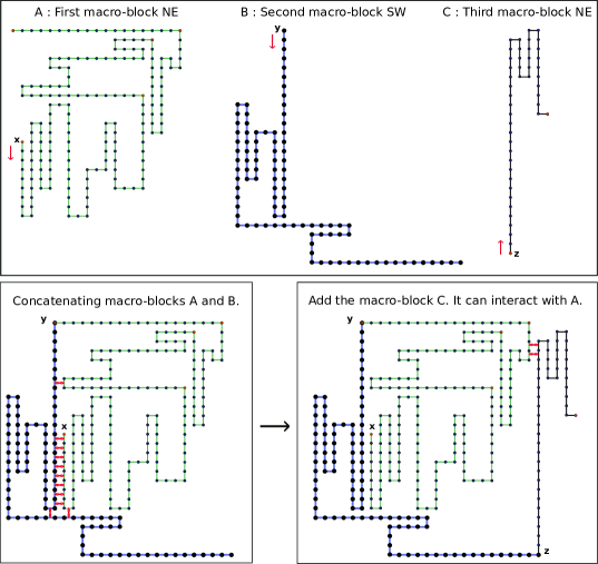
Figure 5. Decomposition of a prudent walk into macro-blocks. In the picture we have a sequence of three macro-blocks, $A,B,\,\text{and}\,C$. The first macro-block (A) has a NE-orientation. The second block (B) has a SW-orientation and it is compatible with the first macro-block, that is, the prudent condition is satisfied. This allows us to concatenate A with B. The third macro-block (C) has a NE-orientation and it satisfies the compatibly condition with $A\oplus B$. The interaction between macro-blocks are highlighted in red.

Lemma 4.8.

Let $L$ be the path length. Then the number of macro-blocks composing the path is bounded from above by $\mathcal{O}(\sqrt{L})$.

Proof.

Pick $w\in\Omega_{L}$, and let $r$ be the number of macro-blocks in $w$. For $j\in\{1\dots,r\}$, we denote by $R_{j}$ the smallest rectangle containing the first $j$ macro-blocks of $w$. In order to complete the $j$-th macro-block and to start a new one, the path should either cross $R_{j}$ horizontally and increase the width of $R_{j}$ by at least $1$ or vertically and increase the height of $R_{j}$ by at least $1$. Therefore, we define $n_{v}$ the number of times that a macro-block ends with a vertical cross, and $n_{h}$ its horizontal counterpart. As a consequence, by keeping in mind that $w$ has length $L$, it must hold that

$$\sum_{i=1}^{n_{v}}i+\sum_{j=1}^{n_{h}}j\leq L.$$ (4.6)

From (4.6) it comes that $n_{v}(n_{v}+1)+n_{h}(n_{h}+1)\leq 2L$ and therefore $n_{v}^{2}+n_{h}^{2}\leq 2L$. Under such condition, the quantity $n_{v}+n_{h}$ is maximal when $n_{v}=n_{h}=\sqrt{L}$. Thus, the number of macro-blocks made by $w$ is not larger than $2\sqrt{L}$.

∎

5. Proof of Theorem 2.2

In this section we prove Theorem 2.2 subject to Theorem 2.1 which ensures that $\mathrm{F}^{\texttt{NE}}(\beta)=\mathrm{F}(\beta)$ for any $\beta\in[0,\infty)$. Therefore it is sufficient to prove Theorem 2.2 for NE-PSAW. Theorem 2.1 will be proven in Section 6.

We consider the free energy of NE-IPSAW

$$\mathrm{F}^{\texttt{NE}}(\beta):=\lim_{L\to\infty}\frac{1}{L}\log\mathrm{Z}_{\beta,\,L}^{\texttt{NE}}.$$ (5.1)

In Section 8 we prove that this limit exists and is finite. Let us observe that, by Remark 4.6, $\mathrm{F}^{\texttt{NE}}(\beta)\geq\mathrm{F}^{\texttt{IPDSAW}}(\beta)$, thus it follows that $\mathrm{F}^{\texttt{NE}}(\beta)\geq\beta$ cf. (1.9) in Carmona et al., (2016). To complete the proof of Theorem 2.2 we have to show that there exists a $\beta_{0}$ such that $\mathrm{Z}_{\beta,\,L}^{\texttt{NE}}\leq e^{\beta(L+o(L))}$ for any $\beta\geq\beta_{0}$ and $L\in\mathbb{N}$. To that purpose we disintegrate the partition function $\mathrm{Z}_{\beta,\,L}^{\texttt{NE}}$ by using the decomposition of any $L$-step NE-PSAW path $\pi$ into a family of oriented blocks $(\pi_{1},\dots,\pi_{r})$ with $r\leq L/4$ (cf. Definition 4.3). As displayed in (4.3), we can distinguish between 4 types of NE-PSAW paths depending on the orientation of their first and last oriented block. For simplicity we will only consider $\widehat{Z}_{\beta,\,L}^{\,\,\texttt{NE}}$ which is computed by restricting the partition function to those paths starting with a west-east block and ending with a south-north block (this corresponds to the first decomposition in (4.3)). The contribution to $Z_{\beta,\,L}^{\texttt{NE}}$ of those path satisfying one of the $3$ other possible decompositions in (4.3) are handled similarly. Therefore,

$$\widehat{Z}_{\beta,L}^{\,\,\texttt{NE}} =\sum_{r\in 2\mathbb{N}}\sum_{t_{1}+\dots+t_{r}=L}\sum_{(\pi_{1},\dots,\pi_{r})\in\mathcal{O}_{t_{1},*}^{\to,+}\times\,\mathcal{O}_{t_{2}}^{\uparrow,+}\times\dots\times\,\mathcal{O}_{t_{r-1}}^{\to,+}\times\,\mathcal{O}_{t_{r},\square}^{\uparrow,+}}\exp\bigg{\{}\,\beta\sum_{j=1}^{r}H(\pi_{i})+\beta\ \Phi(\pi_{1},\dots,\pi_{r})\bigg{\}},$$ (5.2)

where $\Phi(\pi_{1},\dots,\pi_{r})$ is a suitable function that takes into account the interactions between different oriented blocks, i.e., counts the number of self-touchings involving monomers belonging to two different oriented blocks.

Henceforth, for every $i\in\{1,\dots,r\}$ we let $d_{i}$ (respectively $f_{i}$) be the first stretch (resp. last stretch) of $\pi_{i}$ and we let $N_{i}$ be the number of stretches constituting $\pi_{i}$. We note that $\phi(\pi_{1},\dots,\pi_{r})$ can be computed by summing for $i=1,\dots,r-1$ the number of self-touchings between $\pi_{i+1}$ and the sub-path $\pi_{1}\oplus\dots\oplus\pi_{i}$. Moreover, the prudent condition implies that $\pi_{i+1}$ can interact with $\pi_{1}\oplus\dots\oplus\pi_{i}$ only through $\pi_{i-1}$ and $\pi_{i}$. To be more specific (see Figure 4), the self-touchings between $\pi_{i}$ and $\pi_{i+1}$ may only happen between $d_{i+1}$ (the first stretch of $\pi_{i+1}$) and some of the inter-stretches of $\pi_{i}$ (whose number is denoted by $\tilde{N}_{i}$), while the self-touchings between $\pi_{i-1}$ and $\pi_{i+1}$ may only happen between $d_{i+1}$ and $f_{i-1}$ (the last stretch of $\pi_{i-1}$). Of course, for every $i\in\{0,\dots,r-1\}$, the number of inter-stretches in $\pi_{i}$ that may interact with $d_{i+1}$ is not larger than the number of inter-stretches in $\pi_{i}$, i.e., $\tilde{N}_{i}\leq N_{i}-1$. By assigning to $\tilde{N}_{i}$ the same sign as $f_{i-1}$, we can check without further difficulty (see Figure 4) that the number of self-touchings between $\pi_{i-1},\pi_{i}$ and $\pi_{i+1}$ is bounded from above by

$$(\tilde{N}_{i}+f_{i-1})\,\tilde{\wedge}\,d_{i+1},$$

where the $\,\tilde{\wedge}\,$ operator is defined in (5.5) below. We stress again that $\tilde{N}_{i}$ and $f_{i-1}$ have the same sign, while $d_{i+1}$ has the opposite orientation. By using the definition of $\,\tilde{\wedge}\,$ in (5.5) and the triangle inequality, we have the following inequality for every $c\in(0,1/2)$, i.e.,

$$(\tilde{N}_{i}+f_{i-1})\,\tilde{\wedge}\,d_{i+1}\,\leq\,\frac{1}{2}|d_{i+1}|+\frac{1}{2}|f_{i-1}|+\left(\frac{1}{2}+c\right)|N_{i}-1|-c\,|f_{i-1}+d_{i+1}|,\qquad i=1,\cdots,r-1,$$ (5.3)

where $f_{0}=0$ by definition. It turns out that the value of $c$ is worthless: in the sequel we choose $c=1/4$. We use (5.3) to conclude that

$$e^{\,\beta\,\Phi(\pi_{1},\dots,\pi_{r})}\leq e^{\,\frac{\beta}{2}\left(|d_{2}|+\cdots+|d_{r}|\right)}e^{\,\frac{\beta}{2}\left(|f_{1}|+\cdots+|f_{r-2}|\right)}e^{\,\frac{3}{4}\,\beta\,\left(N_{1}+\cdots+N_{r}-r\right)}e^{\,-\frac{\beta}{4}\left(|f_{0}+d_{2}|+\cdots+|f_{r-2}+d_{r}|\right)}.$$ (5.4)

At this stage, we let $\mathrm{Q}_{\beta,t,d,f,N}$ be the partition function associated with those oriented blocks made of $N$ stretches $(\ell_{1},\dots,\ell_{N})$, of total length $t$, starting with a stretch $\ell_{1}=d$, finishing with a stretch $\ell_{N}=f$. Since $\mathrm{Q}_{\beta,t,d,f,N}$ is a partition function involving partially directed paths only, we can use the Hamiltonian representation displayed in Carmona et al., (2016) with the help of the operator $\,\tilde{\wedge}\,$: for any pair $(x,y)\in\mathbb{Z}^{2}$ we let

$$x\,\tilde{\wedge}\,y:=\frac{1}{2}\big{(}\,|x|+|y|-|x+y|\,\big{)}=\begin{cases}\min\{|x|,|y|\},&\,\text{if}\,\,xy<0,\\ 0,&\,\text{otherwise}.\end{cases}$$ (5.5)

In such a way for a given sequence of $N$-stretches, $(\ell_{1},\dots,\ell_{N})$, the Hamiltonian in (2.2) becomes

$$\textrm{H}\big{(}(\ell_{1},\dots,\ell_{N})\big{)}={\,\sum_{i=1}^{N-1}\,(\ell_{i}\,\tilde{\wedge}\,\ell_{i+1})}.$$ (5.6)

Since we are looking for an upper bound on $\widehat{Z}_{\beta,\,L}^{\,\,\texttt{NE}}$, we forget about the exit condition that a block must satisfy (cf. Definition 4.3) and we define $\mathrm{Q}_{\beta,\,t,d,f,N}$, on $\mathcal{L}_{N,t}$, the set of all partially-directed paths of length $t$ with $N-1$ inter-stretches. To be more specific, for $N\in\mathbb{N}$ we let

$$\begin{split}&\mathcal{L}_{N,t}\,:=\left\{\ell=(\ell_{1},\dots,\ell_{N})\,:\,\sum_{i=1}^{N}\,|\ell_{i}|=t-N+1\right\},\end{split}$$ (5.7)

and we define

$$\mathrm{Q}_{\beta,t,d,f,N}\,:=\,\sum_{\begin{subarray}{c}\ell\in\mathcal{L}_{N,t}\\ \ell_{1}=d,\ell_{N}=f\end{subarray}}\exp\left\{\,\beta\,\sum_{n=1}^{N-1}\,(\ell_{n}\,\tilde{\wedge}\,\ell_{n+1})\right\}.$$ (5.8)

It follows that an upper bound on $\widehat{Z}_{\beta,\,L}^{\,\,\texttt{NE}}$ can be obtained from (5.2). To that aim, for a given $r\in\{1,\dots,L/4\}$ and $t_{1}+\dots+t_{r}=L$, we rewrite the inner summation in (5.2) depending on the value taken by $(d_{i},f_{i},N_{i})$ for $i\in\{1,\dots,r\}$. We recall that $d_{i}<0$ for $i\geq 2$ and we lighten the notation with

$$\Xi_{(t_{1},\dots,t_{r})}=\Big{\{}(d_{i},f_{i},N_{i})_{i=1}^{r}\colon|d_{i}|+|f_{i}|+N_{i}-1\leq t_{i},\,\,d_{i}<0\,\forall\,i\geq 2,\,\,N_{i}\geq 2\,\forall\,i\neq r\,\Big{\}},$$

where the $(t_{1},\dots,t_{r})$-dependency of $\Xi$ may be omitted when there is no risk of confusion. We plug (5.4) inside (5.2) to obtain

$$\begin{split}\widehat{Z}_{\beta,\,L}^{\,\,\texttt{NE}}\,&\leq\,\sum_{r=1}^{L/4}\sum_{{t_{1}+\cdots+t_{r}=L}}\sum_{(d_{i},f_{i},N_{i})_{i=1}^{r}\in\Xi}\left(\prod_{i=1}^{r}\,\mathrm{Q}_{\beta,\,t_{i},d_{i},f_{i},N_{i}}\right)\,\times\\ &\qquad e^{\,\frac{\beta}{2}\left(|d_{2}|+\cdots+|d_{r}|\right)}e^{\,\frac{\beta}{2}\left(|f_{1}|+\cdots+|f_{r-2}|\right)}e^{\,\frac{3}{4}\,\beta\,\left(N_{1}+\cdots+N_{r}-r\right)}e^{\,-\frac{\beta}{4}\left(|f_{0}+d_{2}|+\cdots+|f_{r-2}+d_{r}|\right)}\end{split}$$ (5.9)

Remark 5.1.

According to Definition 4.4 and 4.3, we want to stress that $\pi_{r}$, the last block of the path, can have zero inter-stretches, i.e., it may happen that $N_{r}=1$. For the other blocks, $\pi_{1},\dots,\pi_{r-1}$, $N_{i}$ must be larger or equal to $2$, because the exit condition (cf. Definition 4.3) implies that each such block contains at least two stretches.

With the help of (5.5) we can rewrite $\mathrm{Q}_{\beta,\,t,d,f,N}$ in (5.8) as

$$\begin{split}\mathrm{Q}_{\beta,\,t,d,f,N}\,&=\,\sum_{\begin{subarray}{c}\ell\in\mathcal{L}_{N,t}\\ \ell_{1}=d,\ell_{N}=f\end{subarray}}\exp\left\{\,\beta\,\sum_{n=1}^{N}\,|\ell_{n}|\,-\frac{\beta}{2}\,\sum_{n=1}^{N-1}\,|\ell_{n}+\ell_{n+1}|\,-\frac{\beta}{2}|f|-\frac{\beta}{2}|d|\right\}.\end{split}$$ (5.10)

Recall (5.7). For every $\ell\in\mathcal{L}_{N,t}$, the equality $\sum_{n=1}^{N}\,|\ell_{n}|=t-N+1$ can be plugged into (5.10) to obtain

$$\mathrm{Q}_{\beta,\,t,d,f,N}\,=\,e^{\,\beta\,\left(\,t-N+1-\frac{1}{2}|f|-\frac{1}{2}|d|\,\right)}\,\sum_{\begin{subarray}{c}\ell\in\mathcal{L}_{N,t}\\ \ell_{1}=d,\ell_{N}=f\end{subarray}}\prod_{n=1}^{N-1}\exp\left\{-\frac{\beta}{2}\,|\ell_{n}+\ell_{n+1}|\right\}.$$ (5.11)

According to the method used in (Carmona et al.,, 2016, Section 2.1), the r.h.s. of (5.11) admits a probabilistic representation. Let us introduce a random walk $V:=(V_{i})_{i\in\mathbb{N}}$ with i.i.d. increments $(U_{i})_{i\in\mathbb{N}}$ following a discrete Laplace distribution, i.e.,

$$\mathrm{P}_{\beta}\left(U_{1}=k\right)\,=\,\frac{e^{-\frac{\beta}{2}\,|k|}}{c_{\beta}},\quad k\in\mathbb{Z},$$ (5.12)

where $c_{\beta}$ is the normalization constant, i.e.,

$$c_{\beta}\,=\,\sum_{k\in\mathbb{Z}}e^{-\frac{\beta}{2}\,|k|}\,=\,\frac{1+e^{-\frac{\beta}{2}}}{1-e^{-\frac{\beta}{2}}}.$$ (5.13)

In such a way the relation $V_{i}=(-1)^{i-1}\ell_{i}$ for $i=0,\dots,N$ which is equivalent to

$$U_{i}=(-1)^{i-1}(\ell_{i-1}+\ell_{i}),\quad\text{for}\quad i=1,\cdots,N,$$ (5.14)

with $\ell_{0}=0$, defines a one-to-one map between $\mathcal{L}_{N,t}$ and the set of all possible random walk paths of length $t$ and geometric area $G_{N}(V)$ that satisfies

$$G_{N}(V):=\sum_{n=1}^{N}|V_{n}|=t-N+1.$$ (5.15)

Therefore (5.11) becomes

$$\mathrm{Q}_{\beta,\,t,d,f,N}=c_{\beta}^{N-1}\,e^{\,\beta\,\left(\,t-N+1-\frac{1}{2}|f|-\frac{1}{2}|d|\,\right)}\,{\mathrm{P}_{\beta}\left(\left.G_{N}(V)=t-N+1,\,V_{N}=(-1)^{N-1}f\,\right|\,V_{1}=d\right).}$$ (5.16)

We plug (5.16) into (5.9) and we observe that all the factors $e^{\frac{\beta}{2}|d_{i}|},\,i=2,\dots,r$ and $e^{\frac{\beta}{2}|f_{i}|},\,i=1,\dots,r-2$ in the second line of (5.9), are simplified by the corresponding quantities appearing in the exponential factor of (5.16), with $f=f_{i},\,d=d_{i}$ and $N=N_{i}$. Since $t_{1}+\cdots+t_{r}=L$, we obtain that

$$\begin{split}&\widehat{Z}_{\beta,\,L}^{\,\,\texttt{NE}}\,\leq\,e^{\,\beta L}\,\sum_{r=1}^{L/4}\,\sum_{t_{1}+\cdots+t_{r}=L}\,\sum_{(d_{i},f_{i},N_{i})_{i=1}^{r}\in\Xi}\,{e^{-\frac{\beta}{4}\,(N_{1}+\cdots+N_{r}-r)}c_{\beta}^{N_{1}+\cdots+N_{r}-r}}e^{-\frac{\beta}{2}|d_{1}|}e^{-\frac{\beta}{2}|f_{r}|}e^{-\frac{\beta}{2}|f_{r-1}|}\,\times\\ &\qquad\prod_{i=1}^{r}\,{\mathrm{P}_{\beta}\left(\left.G_{N_{i}}(V)=t_{i}-N_{i}+1,\,V_{N_{i}}=(-1)^{N_{i}-1}f_{i}\,\right|\,V_{1}=d_{i}\right)\,}\prod_{i=0}^{r-2}\,e^{-\frac{\beta}{4}\left(|f_{i}+d_{i+2}|\right)},\end{split}$$ (5.17)

At this stage we consider the homogeneous Markov chain kernel (recall (5.12))

$$\rho(x,y):=\frac{e^{\,-\frac{\beta}{4}\left(|x+y|\right)}}{c_{\beta/2}}=\mathrm{P}_{\beta/2}\left(\left.\,V_{1}=-y\,\right|\,V_{0}=x\right),$$ (5.18)

where the $\beta$ dependency of $\rho$ is dropped for simplicity. We observe that $\rho$ is symetric, i.e. $\rho(x,y)=\rho(-x,-y)$. Since we are working with upper bounds we can safely replace $\beta/2$ in $e^{-\frac{\beta}{2}|f_{r}|},e^{-\frac{\beta}{2}|f_{r-1}|}$ and $e^{-\frac{\beta}{2}|d_{1}|}$ by $\beta/4$ and (5.17) becomes (with $f_{-1}=f_{0}=0$ and $d_{r+1}=d_{r+2}=0$)

$$\begin{split}&\widehat{Z}_{\beta,\,L}^{\,\,\texttt{NE}}\,\leq\,c_{\beta/2}\,e^{\,\beta L}\,\sum_{r=1}^{L}\,{c_{\beta/2}^{r}}\sum_{t_{1}+\cdots+t_{r}=L}\,\sum_{(d_{i},f_{i},N_{i})_{i=1}^{r}\in\Xi}\,{\left(\frac{c_{\beta}}{e^{\frac{\beta}{4}}}\right)^{(N_{1}+\cdots+N_{r}-r)}}\times\\ &\prod_{i=1}^{r}\,\mathrm{P}_{\beta}\left(\left.G_{N_{i}}(V)=t_{i}-N_{i}+1,\,V_{N_{i}}=(-1)^{N_{i}-1}f_{i}\,\right|\,V_{1}=d_{i}\right)\,\,\prod_{i=-1}^{r}\,\rho(f_{i},d_{i+2}).\end{split}$$ (5.19)

Now, we focus on the second line in (5.19), our aim is to concatenate all the even blocks on the one hand, and all the odd blocks on the other hand (see Figure 6). For this purpose, for a given sequence $(N_{1},\dots,N_{r})\in\mathbb{N}^{r}$ and for a given index subset $\mathbf{\nu}=\{\nu_{1},\dots,\nu_{m}\}\subset\{-1,\dots,r\}$ we set

$$\mathbf{N}_{k}:=\sum_{i\in\nu,\,1\leq i\leq k}\,N_{i},\qquad\text{for}\quad k=-1,\dots,r.$$ (5.20)

Note that $\mathbf{N}_{-1}=\mathbf{N}_{0}=0$. We let $(\tilde{\mathrm{P}}_{\beta,\nu},\mathbf{V})$ be a non-homogeneous random walk $\mathbf{V}=(\mathbf{V}_{i})_{i=0}^{\mathbf{N}_{r}+1}$, starting from $0$, for which all increments have law $\mathrm{P}_{\beta}$ except those between $\mathbf{V}_{\mathbf{N}_{i}}$ and $\mathbf{V}_{\mathbf{N}_{i}+1}$ for $i\in\{\nu_{1},\dots,\nu_{m}\}$ that have law $\mathrm{P}_{\beta/2}$ (cf. (5.18)). In other words ,

$$\begin{split}&\tilde{\mathrm{P}}_{\beta,\nu}\Big{(}\mathbf{V}_{\mathbf{N}_{i}+1}=y\,\mid\,\mathbf{V}_{\mathbf{N}_{i}}=x\Big{)}={\mathrm{P}}_{\beta/2}\Big{(}\mathbf{V}_{1}=y\,\mid\,\mathbf{V}_{0}=x\Big{)},\qquad i\in\{\nu_{1},\dots,\nu_{m}\},\\ &\tilde{\mathrm{P}}_{\beta,\nu}\Big{(}\mathbf{V}_{a+1}=y\,\mid\,\mathbf{V}_{a}=x\Big{)}={\mathrm{P}}_{\beta}\Big{(}\mathbf{V}_{1}=y\,\mid\,\mathbf{V}_{0}=x\Big{)},\qquad a\notin\{\mathbf{N}_{\nu_{1}},\dots,\mathbf{N}_{\nu_{m}\}}.\end{split}$$ (5.21)

We set, for $k\in\{-1,\dots,r\}$,

$$\begin{split}&\mathbf{N}_{k}^{e}=\sum_{i\in\{1,\dots,k\}\cap 2\mathbb{N}}\,N_{i}\qquad\text{and}\qquad\mathbf{N}_{k}^{o}=\sum_{i\in\{1,\dots,k\}\cap(2\mathbb{N}-1)}\,N_{i},\end{split}$$ (5.22)

We let $(\tilde{\mathrm{P}}_{\beta}^{e},\mathbf{V}^{e}),\,(\tilde{\mathrm{P}}_{\beta}^{o},\mathbf{V}^{o})$ be two independent Markov chains of law $\tilde{\mathrm{P}}_{\beta}^{e}:=\tilde{\mathrm{P}}_{\beta,\{-1,\dots,r\}\cap 2\mathbb{Z}}$ and $\tilde{\mathrm{P}}_{\beta}^{o}:=\tilde{\mathrm{P}}_{\beta,\{-1,\dots,r\}\cap(2\mathbb{Z}+1)}$ respectively. We have to look at $(\mathbf{V}^{e}_{i})_{i=0}^{\mathbf{N}_{r}^{e}+1}$ and $(\mathbf{V}^{o}_{i})_{i=0}^{\mathbf{N}_{r}^{o}+1}$ as the random walks obtained by concatenating the even blocks and the odd blocks respectively, see Figure 6.

For a random walk trajectory $V\in\mathbb{Z}^{\mathbb{N}}$ and for two indices $i<j$ we let $G_{i,j}(V):=\sum_{s=i}^{j}\,|V_{s}|.$ be the geometric area described by $V$ between $i$ and $j$. We are now ready to concatenate the even blocks and the odd blocks in (5.19). We consider separately the odd and even terms in the second line of (5.19). For the odd terms, since $\rho(x,y)=\rho(-x,-y)$ (cf. (5.18)), and since for any odd index $i\leq r$, $\mathbf{N}_{i}^{o}=\mathbf{N}_{i-2}^{o}+N_{i}$, the odd terms in the integrand of (5.19) can be rearranged as follows ($f_{-1}=f_{0}=d_{r+1}=d_{r+2}=0$ by definition)

$$\begin{split}&\begin{aligned} \prod_{\begin{subarray}{c}i\in\{1,\dots,r\}\\ i\in 2\mathbb{Z}+1\end{subarray}}\,&\mathrm{P}_{\beta}\left(\left.G_{N_{i}}(V)=t_{i}-N_{i}+1,\,V_{N_{i}}=(-1)^{N_{i}-1}f_{i}\,\right|\,V_{1}=d_{i}\right)\\ &\hskip 85.35826pt\times\prod_{\begin{subarray}{c}i\in\{-1,\dots,r\}\\ i\in 2\mathbb{Z}+1\end{subarray}}\,\mathrm{P}_{\beta/2}\Big{(}V_{1}=(-1)^{N_{i}}d_{i+2}\,|\,V_{0}=(-1)^{N_{i}-1}f_{i}\Big{)}\end{aligned}\\ &\qquad=\tilde{\mathrm{P}}_{\beta}^{o}\left(\begin{aligned} &G_{\mathbf{N}_{i-2}^{o}+1,\mathbf{N}_{i}^{o}}(\mathbf{V}^{o})=t_{i}-N_{i}+1,\quad\mathbf{V}_{\mathbf{N}_{i-2}^{o}+1}^{o}=(-1)^{\mathbf{N}_{i-2}^{o}}d_{i},\quad\mathbf{V}_{\mathbf{N}_{i}^{o}}^{o}=(-1)^{\mathbf{N}_{i}^{o}-1}f_{i},\\ &\forall\,i\in\{1,\dots,r\}\cap(2\mathbb{Z}+1)\quad\text{and}\quad\mathbf{V}_{\mathbf{N}_{r}^{o}+1}^{o}=0\end{aligned}\right),\end{split}$$ (5.23)

An analogous decomposition holds true for the even terms in the integrand of (5.19).

With the help of (5.23) we interchange the sum over the $t_{i}$’s with the sum over the $N_{i}$’s in (5.19) and we remove the restriction $t_{1}+\dots+t_{r}=L$ to obtain the following upper bound,

$$\begin{split}&\sum_{t_{1}+\cdots+t_{r}=L}\,\sum_{(d_{i},f_{i},N_{i})_{i=1}^{r}\in\Xi}\,{\left(\frac{c_{\beta}}{e^{\frac{\beta}{4}}}\right)^{(N_{1}+\cdots+N_{r}-r)}}\times\\ &\quad\prod_{i=1}^{r}\,\mathrm{P}_{\beta}\left(\left.G_{N_{i}}(V)=t_{i}-N_{i}+1,\,V_{N_{i}}=(-1)^{N_{i}-1}f_{i}\,\right|\,V_{1}=d_{i}\right)\,\,\prod_{i=-1}^{r}\,\rho(f_{i},d_{i+2})\\ &\leq\sum_{\begin{subarray}{c}N_{1}+\dots+N_{r}\leq L+r,\\ N_{i}\geq 2\,i=1,\dots,r-1\end{subarray}}{\left(\frac{c_{\beta}}{e^{\frac{\beta}{4}}}\right)^{(N_{1}+\cdots+N_{r}-r)}}\times\\ &\quad\sum_{\begin{subarray}{c}t_{i}\colon t_{i}\geq N_{i}-1\\ i=1,\dots,r\end{subarray}}\tilde{\mathrm{P}}_{\beta}^{o}\left(G_{\mathbf{N}_{i-2}^{o}+1,\mathbf{N}_{i}^{o}}(\mathbf{V}^{o})=t_{i}-N_{i}+1,\,\forall\,i\in\{1,\dots,r\}\cap(2\mathbb{Z}+1)\,\text{and}\,\mathbf{V}_{\mathbf{N}_{r}^{o}+1}^{o}=0\right)\\ &\hskip 56.9055pt\times\tilde{\mathrm{P}}_{\beta}^{e}\left(G_{\mathbf{N}_{i-2}^{e}+1,\mathbf{N}_{i}^{e}}(\mathbf{V}^{e})=t_{i}-N_{i}+1,\,\forall\,i\in\{1,\dots,r\}\cap 2\mathbb{Z}\,\text{and}\,\mathbf{V}_{\mathbf{N}_{r}^{e}+1}^{e}=0\right).\end{split}$$ (5.24)

We note that the sum over the $t_{i}$’s in the r.h.s. of (5.24) is bounded from above by $1$. It remains to plug (5.24) into (5.19) in which we have exchanged the summation over the $t_{i}$’s with that over the $N_{i}$’s. This leads to

$$\begin{split}&\widehat{Z}_{\beta,\,L}^{\,\,\texttt{NE}}\,\leq\,c_{\beta/2}e^{\,\beta L}\,\sum_{r=1}^{L/4}\,{c_{\beta/2}^{r}}\sum_{\begin{subarray}{c}N_{1}+\dots+N_{r}\leq L+r,\\ N_{i}\geq 2\,i=1,\dots,r-1\end{subarray}}\,{\left(\frac{c_{\beta}}{e^{\frac{\beta}{4}}}\right)^{(N_{1}+\cdots+N_{r}-r)}}\\ &\qquad\leq c_{\beta/2}e^{\,\beta\,L}\,\left[c_{\beta/2}\sum_{N=0}^{\infty}\left(\frac{c_{\beta}}{e^{\frac{\beta}{4}}}\right)^{N}\right]\sum_{r=0}^{\infty}{c_{\beta/2}^{r}}\left[\sum_{N=1}^{\infty}\left(\frac{c_{\beta}}{e^{\frac{\beta}{4}}}\right)^{N}\right]^{r}.\end{split}$$ (5.25)

At this stage, by using the definition of $c_{\beta}$ in (5.13), there exists $\beta_{0}\in(0,\infty)$ such that $c_{\beta}/e^{\beta/4}<1/4$ and $c_{\beta/2}\leq 2$, for any $\beta>\beta_{0}$. This implies that $\widehat{Z}_{\beta,\,L}^{\,\,\texttt{NE}}\leq C(\beta)\,e^{\,\beta\,L}$ for some suitable constant $C(\beta)\in(0,\infty)$.

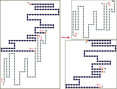
Figure 6. A NE-prudent path made of two south-north blocks (the first and the third, in green) and two west-east blocks (the second and the fourth, in blue). The blocks start at $x,y,z,w$ respectively and their orientation is given by the arrow near to each starting point. Then we can concatenate the even blocks (see top right picture) and the odd blocks (see bottom right picture), obtaining two partially directed self-avoiding path.

6. Proof of Theorem 2.1

To prove Theorem 2.1, we show that for any $\beta\geq 0$ the partition function of IPSAW can be bounded from below and from above by the partition function of NE-IPSAW, by paying at most a sub-exponential price, i.e.,

$$\mathrm{Z}_{\beta,L}^{\texttt{NE}}\leq\mathrm{Z}_{\beta,L}\leq e^{o(L)}\,\mathrm{Z}_{\beta,L}^{\texttt{NE}},\quad\forall\,L\in\mathbb{N},\,\forall\,\beta\in[0,\infty).$$ (6.1)

Where the $o(L)$ depends on $\beta$.

The lower bound in (6.1) is trivial because NE-paths are a particular subclass of prudent paths. The proof of the upper bound is harder and needs some work. In a few word, we will apply a strategy which consists, for every $L\in\mathbb{N}$ and $\beta\in(0,\infty)$, in building a mapping $M_{L}:\Omega_{L}^{\texttt{PSAW}}\to\Omega_{L}^{\texttt{NE}}$ which satisfies the following conditions:

1. There exists a real function $f_{1}$ such that $|(M_{L})^{-1}(\hat{w})|\leq e^{f_{1}(L)},$ where $f_{1}(L)$ is uniform in $\hat{w}\in\Omega_{L}^{\texttt{NE}}$ and $f_{1}(L)=o(L)$,

2. There exists a real function $f_{2}$ such that $H\,(w)-H\,\big{(}M_{L}(w)\big{)}\leq f_{2}(L),$ where $f_{2}(L)$ is uniform in $w\in\Omega_{L}^{\texttt{PSAW}}$ and $f_{2}(L)=o(L)$.

The existence of $(M_{L})_{L\in\mathbb{N}}$ satisfying the aforementioned properties is sufficient to prove the upper bound in (6.1). The dependency in $\beta$ is dropped for simplicity.

We will build the mapping with the help of the macro-block decomposition of every path $w\in\Omega_{L}^{\texttt{PSAW}}$ (recall Section 4.3). By a succession of systematic transformations we will indeed map each macro-block onto an associated NE-macro-block in such a way that the resulting NE-macro-blocks can be concatenated into a NE-prudent path which will be the image of $w$ by $M_{L}$. Then, it will be enough to check that $(M_{L})_{L\in\mathbb{N}}$ satisfies the aforementioned properties.

The first property, (1), will be rigorously proven below and it is mostly a consequence of Lemma 4.8 which states that the macro-block number is at most $\mathcal{O}(\sqrt{L})$. The second property, (2), is the hardest to check. On the energetic point of view, the main difference between a generic prudent paths and their North-East counterpart is that generic paths undergo interactions between macro-blocks. Such interactions turn out to be tuned by the first stretches of each macro-blocks. Moreover, Lemma 4.8 implies that an important loss between $w$ and $M_{L}(w)$ can only be observed when those first stretches are very large. This is the reason why we remove such stretches from the path as soon as they are larger than a prescribed size, e.g., $L^{1/4}$. This only triggers a sub-exponential loss of entropy since those large stretches are at most $L^{3/4}$. It might cause a large loss of energy, but this loss will be compensated by the construction of a large square block (i.e., maximizing the energy) containing all those stretches that we have removed.

We now start with the precise construction of $M_{L}$. For such purpose, we define $4$ sequences of applications that are mapping trajectories onto other trajectories. To be more specific, for every $L\in\mathbb{N}$, we define $5$ sets of trajectories $\mathcal{W}_{i,L},\,i=1,\dots,5$, interpolating $\Omega_{L}^{\texttt{PSAW}}=\mathcal{W}_{1,L}$ with $\Omega_{L}^{\texttt{NE}}=\mathcal{W}_{5,L}$, and $4$ sequences of applications $\psi_{L}^{i}:\mathcal{W}_{i,L}\to\mathcal{W}_{i+1,L}$, cf. Steps 1-4 below. We define $M_{L}$ as the composition of such maps $\psi_{L}^{4},\dots,\psi_{L}^{1}$, i.e., $M_{L}:=\psi_{L}^{4}\circ\psi_{L}^{3}\circ\psi_{L}^{2}\circ\psi_{L}^{1}$. To prove property (1) we show that each $\psi_{L}^{i}$ is sub-exponential, i.e,

Definition 6.1.

The sequence of mappings $(\psi_{L})_{L\in\mathbb{N}}$, with $\psi_{L}\colon\mathcal{W}_{1,L}\to\mathcal{W}_{2,L}$, is sub-exponential if there exist $c_{1},c_{2}\in(0,\infty)$ and $\alpha\in[0,1)$ such that for every $L\in\mathbb{N}$ and every $w\in\mathcal{W}_{2,L}$

$$|(\psi_{L})^{-1}(w)|\leq c_{1}e^{c_{2}L^{\alpha}}.$$ (6.2)

In Step $5$ we complete the proof by showing that such $M_{L}$ satisfies also the second property (2).

6.1. Step 1

Let $w\in\Omega_{L}^{\texttt{PSAW}}$ be a prudent path. We can decompose $w$ into a sequence of macro-blocks, $\Lambda=(\Lambda_{1},\dots,\Lambda_{m})$, where $m=m(w)\in\mathbb{N}$, cf. (4.5) and Section 4.3. We observe that each macro-block $\Lambda_{i}\in\Omega_{L_{i}}^{x_{i}}$, with $x_{i}\in\{\text{NE, NW, SE, SW}\}$ and $L_{i}\in\mathbb{N}$ such that $L_{1}+\dots+L_{m}=L$. Each macro-block $\Lambda_{i}$ can be decomposed into a sequence of blocks $(\pi_{1}^{i},\dots,\pi_{r_{i}}^{i})$, cf. Section 4.2. We stress that both such decompositions are uniques. For every $i=1,\dots,m$, we consider separately the subsequence of blocks with odd indices, i.e., $\pi^{(\textbf{o}),i}:=(\pi_{k}^{i})_{k\in\{1,\dots,r_{i}\}\cap(2\mathbb{N}-1)}$ and the subsequence of blocks with even indices, i.e., $\pi^{(\textbf{e}),i}:=(\pi_{k}^{i})_{k\in\{1,\dots,r_{i}\}\cap 2\mathbb{N}}$. We apply to each of them the following procedure (1-4), drawn in Figure 7. In the sequel, this procedure will be referred to as the large stretches removing procedure.

1. We consider the first macro-block $\Lambda_{1}$ and the odd block subsequence, $\pi^{(\textbf{o}),1}=(\pi_{k}^{1})_{k\in\{1,\dots,r_{1}\}\cap(2\mathbb{N}-1)}$. We start by considering the first stretch of the first block, $\pi_{1}^{1}$. If this stretch is not larger than $L^{1/4}$ we stop the procedure for the subsequence $\pi^{(\textbf{o}),1}$ and we jump to (2). Otherwise, if the first stretch is larger than $L^{1/4}$, we pick it off, and we reapply the procedure to the next stretch of the block.

   It may be that the procedure leads to removing all the stretches in the first block. In such case we re-apply the same procedure to the next block of $\pi^{(\textbf{o}),1}$ and so on, until we find the first stretch smaller than $L^{1/4}$. For instance, in the odd subsequence, if we have entirely removed the first block, then we re-apply the procedure to the third block. If none of the stretches in the subsequence $\pi^{(\textbf{o}),1}$ is smaller than $L^{1/4}$, then the whole subsequence of blocks is removed and we stop the procedure for the subsequence.

2. We apply the procedure (1) to the even block subsequence, $\pi^{(\textbf{e}),1}=(\pi_{k}^{1})_{k\in\{1,\dots,r_{1}\}\cap 2\mathbb{N}}$, i.e., we start with the procedure (1) by considering the first stretch of the second block, $\pi_{2}^{1}$.

3. We apply the procedure (1) to the very last block of the macro-block $\Lambda_{1}$ (if it has not been already modified).

   We will see in Step $3$ below the importance of applying the large-stretch removing procedure to the very last block.

4. We repeat (1-3) for the macro-blocks $\Lambda_{2},\dots,\Lambda_{m}$.

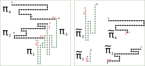
Figure 7. A NE-prudent path decomposed into $4$ blocks $(\pi_{1},\pi_{2},\pi_{3},\pi_{4})$. We apply the large-stretch removing procedure. The first $2$ stretches of $\pi_{1}$ are longer than $L^{1/4}$, therefore we pick them off. The third stretch is smaller than $L^{1/4}$ and thus we stop the procedure on the odd subsequence. We apply the large-stretch removing procedure to the even subsequence. In this case we remove only the first stretch of $\pi_{2}$ and we stop the procedure. Since $\pi_{4}$ is the last block of the trajectory we re-apply the large-stretch removing procedure to $\pi_{4}$. Also in this case we remove only the first stretch. The result is the block sequence $(\tilde{\pi}_{1},\tilde{\pi}_{2},\tilde{\pi}_{3},\tilde{\pi}_{4})$.

Remark 6.2.

We note that picking off stretches does not change the exit condition, cf. Definition 4.3. To be more precise, given an oriented block with $N$-stretches, $(\ell_{1},\dots,\ell_{N})$, if we remove the first $k$-stretches ($k<N$), then the path obtained by concatenating $(\ell_{k+1},\dots,\ell_{N})$ still satisfies the same exit condition. The exit condition indeed means that $\ell_{1}+\dots+\ell_{N}>\max\{0,\ell_{1},\dots,\ell_{1}+\dots+\ell_{N-1}\}$ and therefore $\ell_{k+1}+\dots+\ell_{N}>\max\{0,\ell_{k+1},\dots,\ell_{k+1}+\dots+\ell_{N-1}\}$. However, picking off stretches can change the initial condition of a block, it could happen that the first stretch of the modified block is positive, i.e., $\ell_{k+1}\geq 0$.

At this stage, we need to give a mathematical definition of the large stretch removing procedure. To that aim, for every $L\in\mathbb{N}$, we denote by $\psi_{L}^{1}:\Omega_{L}^{\texttt{PSAW}}\to\psi_{L}^{1}\big{(}\Omega_{L}^{\texttt{PSAW}}\big{)}$ the map that realizes the large stretches removing procedure. At the end of the present section, we will show that $(\psi_{L}^{1})_{l\geq 1}$ is sub-exponential. However, for the sake of conciseness, the fine details of the proof will be displayed only in the case for which we do not reapply the large stretch removing procedure to modify the very last block of each macro-block. The proof in that case is very similar, see Remark 6.5 below.

6.1.1. Large stretch removing procedure in a single macro-block

We pick $l\in\mathbb{N}$ and an orientation $x\in\{\text{NE, NW, SE, SW}\}$. In the present section, we define the large stretch removing procedure on those macro-blocks in $\Omega_{l}^{x}$. To that aim, we define with (6.3–6.5) an application $\mathcal{T}_{l,L}:\Omega_{l}^{x}\mapsto\Omega^{l,x}_{\leq,L}$ that performs Procedure (1), i.e., removes the large stretches in a single macro-block. A rigorous definition of the image set $\Omega^{l,x}_{\leq,L}$ will be provided in Definition 6.4 below.

Before defining $\mathcal{T}_{l,L}$, let us briefly recall that we can associate with any arbitrary macro-block $\lambda\in\Omega_{l}^{x}$ an unique block sequence $(\pi_{1},\dots,\pi_{r})$, with $r=r(\lambda)$. In particular it holds that $\lambda=\pi_{1}\oplus\dots\oplus\pi_{r}$, see Section 4.2. Therefore, in the rest of the section, we identify the macro-block with its block decomposition, i.e., $\lambda=(\pi_{1},\dots,\pi_{r})$. For every $i\in\{1,\dots,r\}$, we let $N_{i}=N_{i}(\lambda)$ be the number of stretches in the $i$-th block (thus, cf. Section 4.1, the number of inter-stretches is $N_{i}-1$), and we let $(\ell_{1}^{(i)},\cdots,\ell_{N_{i}}^{(i)})$ be the sequence of stretches in the $i$-th block. Since the sequence of stretches identifies the block, with a slight abuse of notation, we write $\pi_{i}=(\ell_{1}^{(i)},\cdots,\ell_{N_{i}}^{(i)})$. The sequence of blocks $(\pi_{1},\dots,\pi_{r})$ can be partitioned into two subsequences $\mathbf{\pi^{(o)}}=(\pi_{i})_{i\in\{1,\dots,r\}\cap(2\mathbb{N}-1)}$ and $\mathbf{\pi^{(e)}}=(\pi_{i})_{i\in\{1,\dots,r\}\cap 2\mathbb{N}}$.

At this stage, we are ready to introduce the specific notations for the large stretches removing procedure. We let $k_{1},k_{2}=k_{1}(\lambda),k_{2}(\lambda)\in\{1,\dots,r\}$ be the indices of the last block modified by the large stretches removing procedure in the odd subsequence and in the even subsequence respectively (cf. (1)). Analogously, let $j_{1}=j_{1}(\lambda)\in\{0,\dots,N_{k_{1}}\}$ and $j_{2}=j_{2}(\lambda)\in\{0,\dots,N_{k_{2}}\}$ be the index of the last stretch we removed in $\pi_{k_{1}}$ and $\pi_{k_{2}}$ respectively. By definition of $r,k_{1},k_{2},j_{1},j_{2},N_{m}$ it holds that (note that the $\lambda$ dependency is dropped for simplicity)

$$|\ell_{n}^{(m)}|>L^{1/4},\quad\text{for}\quad m\in\{1,\dots,k_{1}-1\}\cap(2\mathbb{N}-1),\ n\in\{1,\dots,N_{m}\},$$ (6.3)

$$|\ell_{n}^{(k_{1})}|>L^{1/4},\quad\text{for}\quad n\in\{1,\dots,j_{1}\},$$

$$|\ell_{j_{1}+1}^{(k_{1})}|\leq L^{1/4};$$

$$|\ell_{n}^{(m)}|>L^{1/4},\quad\text{for}\quad m\in\{1,\dots,k_{2}-1\}\cap 2\mathbb{N},\ n\in\{1,\dots,N_{m}\},$$ (6.4)

$$|\ell_{n}^{(k_{2})}|>L^{1/4},\quad\text{for}\quad n\in\{1,\dots,j_{2}\},$$

$$|\ell_{j_{2}+1}^{(k_{2})}|\leq L^{1/4}.$$

We let $\mathcal{T}_{l,L}(\lambda)$ be the sequence of blocks remaining once the large stretch removing procedure in the macro-block $\lambda$ is complete. To be more specific, the subsequence of odd blocks $(\mathcal{T}_{l,L}(\lambda)_{i})_{i\in\{1,\cdots,r\}\cap(2\mathbb{N}-1)}$ is defined as

$$\begin{split}&\mathcal{T}_{l,L}(\lambda)_{k}=\emptyset,\quad\forall\,k\in\{1,\dots,k_{1}-1\}\cap(2\mathbb{N}-1),\\ &\mathcal{T}_{l,L}(\lambda)_{k_{1}}=\Big{(}\ell_{j_{1}+1}^{(k_{1})},\dots,\ell_{N_{k_{1}}}^{(k_{1})}\Big{)},\\ &\mathcal{T}_{l,L}(\lambda)_{k}=\pi_{k},\quad\forall\,k\in\{k_{1}+1,\dots,r\}\cap(2\mathbb{N}-1).\end{split}$$ (6.5)

The subsequence of even blocks $(\mathcal{T}_{l,L}(\lambda)_{i})_{i\in\{1,\dots,r\}\cap 2\mathbb{N}}$ is defined in the same way.

Remark 6.3.

We stress that if we start with a sequence of blocks $\lambda=(\pi_{1},\dots,\pi_{r})\in\Omega_{l}^{x}$, then, in general, it is not true that the sequence $\mathcal{T}_{l,L}(\lambda)=(\mathcal{T}_{l,L}(\lambda)_{1},\dots,\mathcal{T}_{l,L}(\lambda)_{r})$ we defined in (6.5) is still a decomposition of a $x$-prudent path, i.e., $\mathcal{T}_{l,L}(\lambda)$ may not belong to $\Omega_{s}^{x}$, for any $s\leq l$. For this reason we define here below a new set of oriented paths, $\Omega_{\leq,L}^{l,x}$, which gathers the images of all paths in $\Omega_{l}^{x}$ through $\mathcal{T}_{l,L}$.

Definition 6.4.

We say that a block sequence $\lambda=(\pi_{1},\dots,\pi_{r}),\,r\in\{0,\dots,L\}$ belongs to $\Omega_{\leq,L}^{l,x}$ if and only if

• $r\leq L$ and there exists $k_{1}\in 2\mathbb{N}-1$ and $k_{2}\in 2\mathbb{N}$ such that $k_{1},k_{2}\leq\max\big{\{}r,\frac{l}{L^{1/4}}\big{\}}$ and $\pi_{i}=\emptyset$ for $i\in\{1,\dots,k_{1}-2\}\cap 2\mathbb{N}-1$ and for $i\in\{1,\dots,k_{2}-2\}\cap 2\mathbb{N}$, whereas $\pi_{i}\neq\emptyset$ for $i\in\{k_{1},\dots,r\}\cap 2\mathbb{N}-1$ and for $i\in\{k_{2},\dots,r\}\cap 2\mathbb{N}$.

• the $x$ orientation is respected (cf. Section 4.2), e.g., in the case of $x=\texttt{NE}$, then, every $\pi_{i}$ with ${i\in\{k_{1},\dots,r\}\cap(2\mathbb{N}-1)}$ is south-north (resp. west-east) and every $\pi_{i}$ with ${i\in\{k_{2},\dots,r\}\cap 2\mathbb{N}}$ is west-east (resp. south-north).

• There is no restriction on the orientation and on the length of the first stretch of $\pi_{k_{1}}$ and $\pi_{k_{2}}$.

• The total length (the sum of the length of every stretches in $(\pi_{1},\dots,\pi_{r})$) is smaller than $l$.

We conclude this section with the computation of an upper bound on the cardinality of the ancestors of an arbitrary $\gamma\in\Omega_{\leq,L}^{l,x}$ by $\mathcal{T}_{l,L}$. We denote by $h$ the total length of $\gamma$. Let $\lambda\in\Omega_{l}^{x}$ be an ancestor of $\gamma$ by $\mathcal{T}_{l,L}$. The total length of those stretches removed from $\lambda$ by $\mathcal{T}_{l,L}$ to get $\gamma$ necessarily equals $l-h$. By definition, cf. (6.5), the number of empty blocks in $\gamma$ is $k^{{}^{\prime}}_{1}:=\frac{k_{1}-1}{2}$ (resp. $k^{{}^{\prime}}_{2}:=\frac{k_{2}-2}{2}$) for the odd subsequence (resp. for the even subsequence) of blocks. Therefore, since $\mathcal{T}_{l,L}$ may remove only stretches larger than $L^{1/4}$, the number $v$ of stretches removed from $\lambda$ to get $\gamma$ satisfies $k^{{}^{\prime}}_{1}+k^{{}^{\prime}}_{2}+2\leq v\leq(l-h)/L^{1/4}$. This suffices to write the following upper bound

$$\Big{|}(\mathcal{T}_{l,L})^{-1}(\gamma)\Big{|}\leq\sum_{v=k^{{}^{\prime}}_{1}+k^{{}^{\prime}}_{2}+2}^{(l-h)/L^{1/4}}2^{v}\,\binom{l-h}{v}\,\binom{v}{k^{{}^{\prime}}_{1}+k^{{}^{\prime}}_{2}+2}.$$ (6.6)

The summation in (6.6) runs over $v$ which stands for the number of stretches removed from $\lambda$. Let us explain (6.6). Once $v$ is chosen, reconstructing $\lambda$ requires to choose the length of each removed stretches and these choices are less than the binomial factor $\binom{l-h}{v}$. Once, the length of each removed stretch is chosen, one has to chose their orientations which gives at most $2^{v}$ choices. Finally, those deleted stretches have to be distributed among the $k^{{}^{\prime}}_{1}+k^{{}^{\prime}}_{2}+2$ blocks in $\gamma$ that have to be completed by other stretches to recover $\lambda$. This gives rise to the term $\binom{v}{k^{{}^{\prime}}_{1}+k^{{}^{\prime}}_{2}+2}$. Then, the fact that $k^{{}^{\prime}}_{1}+k^{{}^{\prime}}_{2}+2\leq(l-h)/L^{1/4}$ allows us to bound from above the r.h.s. in (6.6) by

$$\Big{|}(\mathcal{T}_{l,L})^{-1}(\gamma)\Big{|}\leq e^{c_{0}l\log(L)/L^{1/4}},$$ (6.7)

for some constant $c_{0}\in(0,\infty)$.

6.1.2. Large stretch removing procedure for a generic prudent path.

We are ready to define the map $\psi_{L}^{1}$, which defines the large stretch removing procedure applied to generic prudent path. We recall equation (4.5), which asserts that a path $w\in\Omega_{L}^{\texttt{PSAW}}$ can be decomposed into $m=m(w)\in\mathbb{N}$ macro-blocks $(\Lambda_{1},\dots,\Lambda_{m})$. Such macro-block decomposition is an element of $\Theta_{m,L}$ and each macro-block belongs to some $\Omega_{t_{i}}^{x_{i}}$ (see (4.4)) with $t_{1}+\dots+t_{m}=L$. Thus, we define $\psi_{L}^{1}$ by applying, for every $i\leq m$, the map $\mathcal{T}_{t_{i},L}$ to $\Lambda_{i}$, i.e.,

$$\psi_{L}^{1}(w):=\big{(}\mathcal{T}_{t_{1},L}(\Lambda_{1}),\dots,\mathcal{T}_{t_{m},L}(\Lambda_{m})\big{)}.$$ (6.8)

The image set of $\Omega_{L}^{\texttt{PSAW}}$ by $\psi_{L}^{1}$ is is therefore $\mathcal{W}_{2,L}:=\bigcup_{m\in\mathbb{N}}\psi_{L}^{1}\big{(}\Theta_{m,L}\big{)}$ which is a subset of

$$\bigcup_{m\in\mathbb{N}}\bigcup_{L_{1}+\dots+L_{m}=L}\bigcup_{\begin{subarray}{c}(x_{i})_{i=1}^{m}\in\{\texttt{NE},\texttt{NW},\texttt{SE},\texttt{SW}\}\\ x_{i-1}\neq x_{i}\end{subarray}}\,\Omega_{\leq,L}^{L_{1},x_{1}}\times\dots\times\Omega_{\leq,L}^{L_{m},x_{m}}.$$ (6.9)

Let us observe that the union over $m$ is finite, because, by Lemma 4.8, the number of macro-blocks $m$ is at most $cL^{1/2}$, for some universal constant $c\in(0,\infty)$. Moreover, let us observe that (6.9) is not a disjoint union.

The step will be completed once we show that $\psi_{L}^{1}$ is sub-exponential. To that aim, we need an upper bound on the cardinality of $(\psi_{L}^{1})^{-1}(\tilde{\Lambda})$ that is uniform on the choice of $\tilde{\Lambda}\in\psi_{L}^{1}\big{(}\Omega_{L}^{\texttt{PSAW}}\big{)}$. Thus, we pick $\tilde{\Lambda}\in\psi_{L}^{1}\big{(}\Omega_{L}^{\texttt{PSAW}}\big{)}$ and we consider its macro-block decomposition $(\tilde{\Lambda}_{1},\dots,\tilde{\Lambda}_{m})$. Before counting the number of ancestors of $\tilde{\Lambda}$ by $\psi_{L}^{1}$, one should note that $\tilde{\Lambda}$ may belong to more than one set of the form $\Omega_{\leq,L}^{L_{1},x_{1}}\times\dots\times\Omega_{\leq,L}^{L_{m},x_{m}}$. However, since $m=\mathcal{O}(L^{1/2})$ (cf. Lemma 4.8) and since $L_{1}+\dots+L_{m}=L$, the number of such sets is bounded from above by $\sum_{m=1}^{c\sqrt{L}}\binom{L}{m}$, for some $c\in(0,\infty)$. This quantity is less than $c\sqrt{L}\binom{L}{c\sqrt{L}}\leq e^{2c\sqrt{L}\log(L)}$. It remains to count the number of ancestors of $\tilde{\Lambda}$ within a given $\Omega_{L_{1}}^{x_{1}}\times\dots\times\Omega_{L_{m}}^{x_{m}}$. By (6.7) above, this is at most $e^{c_{0}L_{1}\log(L)/L^{1/4}}\times\dots\times e^{c_{0}L_{m}\log(L)/L^{1/4}}$ which again is smaller than $e^{c_{0}L^{3/4}\log(L)}$. This suffices to conclude that $\psi_{L}^{1}$ is sub exponential.

Remark 6.5.

When we prove that $\psi_{L}^{1}$ is sub exponential, we have not taken into account the fact that the large stretch removing procedure should also be applied to the very last block of each macro-block. However, this affects only marginally our computations and does not modify the sub-exponentiality of $\psi_{L}^{1}$. To be more precise, if we also modify the very last block in any macro-block, then to bound from above the number of ancestors of $\tilde{\Lambda}$ by $\psi_{L}^{1}$, we consider separately two parts. In the first part, we apply the large stretches removing procedure to each macro-block without consider the very last block of any macro-block. This part has been already considered in the discussion above, which gave rise to (6.6) and (6.7). Then we consider the large stretches removing procedure apply only to any last block of any macro-block. It is not difficult to check that (6.6) provides an upper bound also for this part of the procedure. Therefore, we conclude that also in this general case (6.7) still holds up to a constant.

6.2. Step 2

In Step 1 we considered $w\in\Omega_{L}^{\texttt{PSAW}}$ and we decomposed it into a sequence of macro-blocks, cf. (4.5), $\Lambda=(\Lambda_{1},\dots,\Lambda_{m})$, where $m=m(w)\in\mathbb{N}$. We let $(\tilde{\Lambda}_{1},\dots,\tilde{\Lambda}_{m})=\psi_{L}^{1}(w)$ be the result of the large stretch removing procedure. Each $\tilde{\Lambda}_{i}$ is defined by a sequence $(\tilde{\pi}_{1}^{i},\dots,\tilde{\pi}_{r_{i}}^{i})$ which is not necessary concatenable, cf. Remark 6.3 and Section 4. In this step we aim at modifying all the sequences $(\tilde{\pi}_{1}^{i},\dots,\tilde{\pi}_{r_{i}}^{i})$, for $i=1,\dots,m$, in order to recover a concatenable block sequence. In the sequel this procedure will be referred to as the concatenating block procedure.

Our procedure $\psi_{L}^{2}$ acts on $\mathcal{W}_{2,L}$ (recall (6.9)). To be more specific, $\psi_{L}^{2}$ takes as an argument an element

$$\tilde{\Lambda}=(\tilde{\Lambda}_{1},\dots,\tilde{\Lambda}_{m})\in\Omega_{\leq,L}^{L_{1},x_{1}}\times\dots\times\Omega_{\leq,L}^{L_{m},x_{m}}$$

where $m\leq cL^{1/2}$, where $(L_{1},\dots,L_{m})$ is a sequence of length such that $L_{1}+\dots+L_{m}=L$, where $(x_{1},\dots,x_{m})$ is a sequence of orientations and where we keep in mind that $\tilde{\Lambda}$ is in the image set of $\psi_{L}^{1}$ . As a result, $\psi_{L}^{2}$ provides us with a sequence of macro-blocks

$$\psi_{L}^{2}(\tilde{\Lambda})=\hat{\Lambda}=(\hat{\Lambda}_{1},\dots,\hat{\Lambda}_{m})$$

where, for every $i\leq m$, $\hat{\Lambda}_{i}\in\Omega_{t_{i}}^{x_{i}}$ with $t_{i}$ the total length of $\tilde{\Lambda}_{i}$.

We describe the procedure on a single modified macro-block $\tilde{\Lambda}$ in Section 6.2.1 below. Later on, we generalize the procedure to the whole block-sequence in Section 6.2.2.

6.2.1. Concatenating block procedure in a single macro-block

We pick $h\leq l\in\mathbb{N}$ and consider $\tilde{\lambda}=(\tilde{\pi}_{1},\dots,\tilde{\pi}_{r})\in\Omega^{l,x}_{\leq,L}$ such that the total length of $\tilde{\lambda}$ equals $h$.

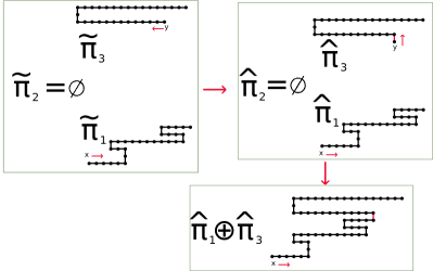
Figure 8. We consider a sequence $(\tilde{\pi}_{1},\tilde{\pi}_{2},\tilde{\pi}_{3})$ provided by the large stretch removing procedure in Step 2. In this case we have that the large stretch removing procedure has removed the block $\tilde{\pi}_{2}$. We modify the first step of the fist stretch of $\tilde{\pi}_{3}$ in order to appear artificially an inter-stretch. In such a way we can safely concatenate the blocks $\hat{\pi}_{1}$ with $\hat{\pi}_{3}$ in a unique block $\hat{\pi}_{1}\oplus\hat{\pi}_{3}$.

Recall the definition of $k_{1}(\tilde{\lambda})$ and $k_{2}(\tilde{\lambda})$ in Definition 6.4. By Remark 6.2 it turns out that $\tilde{\lambda}$ fails to be concatenable only if $|k_{1}-k_{2}|\geq 3$ that is if there exists an $i\leq r$ such that $\tilde{\pi}_{i},\tilde{\pi}_{i+2}\neq\emptyset$ and $\tilde{\pi}_{i+1}=\emptyset$. In such case indeed, if the last stretch of $\tilde{\pi}_{i}$ and the first stretch of $\tilde{\pi}_{i+2}$ have opposite orientations (see Figure 8) then $\tilde{\pi}_{i}$ and $\tilde{\pi}_{i+2}$ are not concatenable. Making $\tilde{\pi}_{i}$ and $\tilde{\pi}_{i+2}$ concatenable possibly requires to slightly modify their structure. To be more specific, if the first stretch of $\tilde{\pi}_{i+2}$ and/or the last stretch of $\tilde{\pi}_{i}$ have zero length, then $\tilde{\pi}_{i+2}$ and $\tilde{\pi}_{i}$ are always concatenable. In this case we do not need to change their structure to make them concatenable. Otherwise, if the first stretch of $\tilde{\pi}_{i+2}$ has non-zero length, then it is always possible to modify the first step in the first stretch of $\tilde{\pi}_{i+2}$ to transform it into an inter-stretch, see Figure 8, and after this simple transformation $\tilde{\pi}_{i}$ and $\tilde{\pi}_{i+2}$ become always concatenable. Thus, in the case where $k_{1}\leq k_{2}-3$ (the case $k_{2}\leq k_{1}-3$ is similar) it suffices to apply the aforementioned transformation to each blocks $\tilde{\pi}_{k_{1}+2},\dots,\tilde{\pi}_{k_{2}-1}$ and to concatenate $\tilde{\pi}_{k_{1}},\dots,\tilde{\pi}_{k_{2}-1}$ into a unique oriented block, say $\hat{\pi}_{1}^{\prime}$. We remove those empty blocks $\tilde{\pi}_{i}$ indexed in $\{1,\dots,k_{1}-2\}\cap 2\mathbb{N}-1$ and in $\{1,\dots,k_{2}-2\}\cap 2\mathbb{N}$ to get finally the concatenable sequence $(\hat{\pi}_{1}^{\prime},\tilde{\pi}_{k_{2}},\dots,\tilde{\pi}_{r})$. The path $\hat{\lambda}:=\hat{\pi}_{1}^{\prime}\oplus\tilde{\pi}_{k_{2}}\oplus\dots\oplus\tilde{\pi}_{r}\in\Omega_{h}^{x}$.

Remark 6.6.

It is important to keep in mind that the concatenable sequence $(\hat{\pi}_{1}^{\prime},\tilde{\pi}_{k_{2}},\dots,\tilde{\pi}_{r})$ is not a standard decomposition of a NE-prudent path, cf. Definition 4.5: in this case we do not have any constriction on the first stretch of $\tilde{\pi}_{k_{2}}$ and $\tilde{\pi}_{r}$ (if the last block was changed by the large stretches removing procedure) other than to be smaller than $L^{1/4}$, cf. Remark 6.2. It is necessary to slightly redefine $\hat{\pi}_{1}^{\prime}$ and $\tilde{\pi}_{k_{2}}$ in order to obtain two proper oriented blocks, say $\hat{\pi}_{1}$ and $\hat{\pi}_{2}$. We also modify $\tilde{\pi}_{r-1}$ and $\tilde{\pi}_{r}$ in the same way to obtain the oriented blocks $\hat{\pi}_{s-1}$ and $\hat{\pi}_{s}$, where $s=(k_{1}+k_{2})/2-2$. We observe that we can do this modification to have that $\hat{\pi}_{s}\subseteq\tilde{\pi}_{r}$. In such a way the block sequence $(\hat{\pi}_{1},\dots,\hat{\pi}_{s})$ is a proper decomposition of a NE-prudent path. We observe that a very crude bound tells us that the number of ancestors of a block by this last transformation is bounded above by its total number of stretches, which is smaller than $l$.

Remark 6.7.

In principle, if the last stretch of $\tilde{\pi}_{i}$ and the first stretch of $\tilde{\pi}_{i+2}$ have both non-zero length and the same orientation, then it would be possible to concatenate $\tilde{\pi}_{i}$ with $\tilde{\pi}_{i+2}$. Anyway, also in this case we modify the $\tilde{\pi}_{i+2}$ structure, as prescribed by the aforementioned transformation. We do that for computational convenience, as it will be clear in (6.10) below.

The procedure described above corresponds to the mapping $\mathcal{R}_{l,L}:\Omega_{\leq,L}^{l,x}\mapsto\cup_{h\leq l}\,\Omega_{h}^{x}$. As we did in Section 6.1.1, we need to conclude this section by computing, for $h\leq l\leq L$ and $x\in\{\text{NE, NW, SE, SW}\}$, the number of ancestors in $\Omega_{\leq,L}^{l,x}$ of a given $\gamma\in\Omega_{h}^{x}$ by $\mathcal{R}_{l,L}$. To that aim, we write $\gamma:=(\hat{\pi}_{1},\dots,\hat{\pi}_{s})\in\Omega_{h}^{x}$ and we consider $\tilde{\lambda}=(\tilde{\pi}_{1},\dots,\tilde{\pi}_{r})\in\Omega_{\leq,L}^{l,x}$ an ancestor of $\gamma$ by $\mathcal{R}_{l,L}$. For simplicity, assume also that $k_{1}=k_{1}(\tilde{\lambda})\leq k_{2}(\tilde{\lambda})=k_{2}$ and recall that, by Definition 6.4, we have necessarily $k_{1},k_{2}\leq\frac{l}{L^{1/4}}$. Thus, we have necessarily that all blocks $(\tilde{\pi}_{1},\tilde{\pi}_{3},\dots,\tilde{\pi}_{k_{1}-2})$ and all blocks $(\tilde{\pi}_{2},\tilde{\pi}_{4},\dots,\tilde{\pi}_{k_{2}-2})$ are empty. Moreover, we explained above that $\hat{\pi}_{1}$ is essentially obtained by modifying the first step of the first stretch of some oriented blocks in $(\tilde{\pi}_{k_{1}},\tilde{\pi}_{k_{1}+2},\dots,\tilde{\pi}_{k_{2}-1})$. This suffices to write the following upper bound

$$\Big{|}(\mathcal{R}_{l,L})^{-1}(\gamma)\Big{|}\leq\sum_{k_{1},k_{2}\leq l/L^{1/4}}l\,2^{|k_{1}-k_{2}|}\binom{l}{\frac{|k_{1}-k_{2}|}{2}},$$ (6.10)

The summation in (6.10) runs over $k_{1},k_{2}$ which provides the number of empty blocks at the beginning of the odd and even sequences of blocks in $\tilde{\lambda}$ and, once $k_{1}$ and $k_{2}$ are chosen, one can reconstruct $(\tilde{\pi}_{k_{1}},\tilde{\pi}_{k_{1}+2},\dots,\tilde{\pi}_{k_{2}-1})$ from $\hat{\pi}_{1}$ by decomposing $\hat{\pi}_{1}$ into $(k_{2}-k_{1})/2$ groups of consecutive stretches. This provides at most $\binom{l}{\frac{|k_{1}-k_{2}|}{2}}$ choices since the number of stretches in $\hat{\pi}_{1}$ is at most $l$. Then we have to take in account the transformation we made on the first step of the first stretch of some oriented blocks in $(\tilde{\pi}_{k_{1}},\tilde{\pi}_{k_{1}+2},\dots,\tilde{\pi}_{k_{2}-1})$. This provide at most two configuration for each such block and thus the factor $2^{|k_{1}-k_{2}|}$. The factor $l$ is due to the fact that we have at most $l$ different way to choose $\tilde{\pi}_{k_{2}-1}$ and $\tilde{\pi}_{k_{2}}$ and $\tilde{\pi}_{r-1}$ and $\tilde{\pi}_{r}$, cf. Remark 6.6. At this stage, it is sufficient to recall that $k_{2}-k_{1}\leq l/L^{1/4}$ to rewrite (6.10) as

$$\Big{|}(\mathcal{R}_{l,L})^{-1}(\gamma)\Big{|}\leq\frac{l^{3}}{L^{1/2}}\,2^{l/L^{1/4}}\,e^{l\log(L)/L^{1/4}}\leq e^{c_{1}l\log(L)/L^{1/4}},$$ (6.11)

for some $c_{1}\in(0,\infty)$.

6.2.2. Concatenating block procedure for a generic path

We are ready to define the map $\psi_{L}^{2}$ on those generic macro-block sequences from $\mathcal{W}_{2,L}$. We recall Definition 6.9, we pick $m\leq c\sqrt{L}$ and $(L_{1},\dots,L_{m})\in\mathbb{N}^{m}$ satisfying $L_{1}+\dots+L_{m}=L$. Then, we pick

$$\tilde{\Lambda}=(\tilde{\Lambda}_{1},\dots,\tilde{\Lambda}_{m})\in\Omega_{\leq,L}^{L_{1},x_{1}}\times\dots\times\Omega_{\leq,L}^{L_{m},x_{m}},$$

and we define $\psi_{L}^{2}$ by applying, for every $i\leq m$, the map $\mathcal{R}_{L_{i},L}$ to $\tilde{\Lambda}_{i}$, i.e.,

$$\psi_{L}^{2}(\tilde{\Lambda}):=\big{(}\mathcal{R}_{L_{1},L}(\tilde{\Lambda}_{1}),\dots,\mathcal{R}_{L_{m},L}(\tilde{\Lambda}_{m})\big{)}.$$ (6.12)

The image set of $\mathcal{W}_{2,L}$ by $\psi_{L}^{2}$ is therefore denoted by $\mathcal{W}_{3,L}$ and it is a subset of

$$\bigcup_{m\leq cL^{1/2}}\,\bigcup_{l_{1}+\dots+l_{m}\leq L}\,\bigcup_{\begin{subarray}{c}(x_{i})_{i=1}^{m}\in\{\texttt{NE},\texttt{NW},\texttt{SE},\texttt{SW}\}\\ x_{i-1}\neq x_{i}\end{subarray}}\,\Omega_{l_{1}}^{x_{1}}\times\dots\times\Omega_{l_{m}}^{x_{m}},$$ (6.13)

where the union over $m$ is truncated at $cL^{1/2}$ thanks to Lemma 4.8.

Remark 6.8.

Let us stress the fact that, as explained in Section 6.1.2 above, a given $\tilde{\Lambda}\in\mathcal{W}_{2,L}$ may well belong to more than one set of the form $\Omega_{\leq,\texttt{vh}}^{L_{1},x_{1}}\times\dots\times\Omega_{\leq,\texttt{vh}}^{L_{m},x_{m}}$. This may be confusing because the definition of $\psi_{L}^{2}$ in (6.12) seems to depend on the choice of $L_{1},\dots,L_{m}$. However, this is not the case because the applications $\mathcal{R}_{l,L}$ do actually not depend on $l$.

The step will be complete once we show that $\psi_{L}^{2}$ is sub-exponential. To that aim, we need an upper bound on the cardinality of $(\psi_{L}^{2})^{-1}(\hat{\Lambda})$ that is uniform on the choice of $\hat{\Lambda}\in\psi_{L}^{2}\big{(}\mathcal{W}_{2,L}\big{)}$. Thus, we pick $\hat{\Lambda}\in\psi_{L}^{2}\big{(}\mathcal{W}_{2,L}\big{)}$ and we consider its macro-block decomposition $(\hat{\Lambda}_{1},\dots,\hat{\Lambda}_{m})$ which belongs to $\Omega_{l_{1}}^{x_{1}}\times\dots\times\Omega_{l_{m}}^{x_{m}}$ for some $l_{1}+\dots+l_{m}\leq L$. Before counting the number of ancestors of $\hat{\Lambda}$ by $\psi_{L}^{2}$, one should note that the ancestors of $\hat{\Lambda}$ may belong to any set of the form $\Omega_{\leq,L}^{L_{1},x_{1}}\times\dots\times\Omega_{\leq,L}^{L_{m},x_{m}}$ with $L_{1}+\dots+L_{m}\leq L$ and $L_{i}\geq l_{i}$ for every $i\leq m$. Again, since $m\leq c\sqrt{L}$, the number of such sets is bounded above by $\binom{L}{c\sqrt{L}}\leq e^{c\sqrt{L}\log(L)}$. It remains to count the number of ancestors of $\hat{\Lambda}$ within a given $\Omega_{\leq,L}^{L_{1},x_{1}}\times\dots\times\Omega_{\leq,L}^{L_{m},x_{m}}$ and by (6.11) above, this is at most $e^{c_{1}L_{1}\log(L)/L^{1/4}}\times\dots\times e^{c_{1}L_{m}\log(L)/L^{1/4}}$ which again is smaller than $e^{c_{1}L^{3/4}\log(L)}$. This suffices to conclude that $\psi_{L}^{2}$ is sub exponential.

Step 3

In this step we consider a macro-block sequence $(\hat{\Lambda}_{1},\dots\hat{\Lambda}_{m})\in\mathcal{W}_{3,L}$ and we begin by modifying each macro-block $\hat{\Lambda}_{i}$ in order to recover a sequence of concatenable macro-blocks with only NE-orientations. Then we concatenate those modified north-east macro-blocks to recover a two sided path. In the sequel we refer to such procedures as macro-block concatenating procedure.

This procedure is defined through the function $\psi_{L}^{3}$, which acts on $\mathcal{W}_{3,L}$ (recall (6.13)). To be more specific, $\psi_{L}^{3}$ takes as an argument an element

$$\hat{\Lambda}=(\hat{\Lambda}_{1},\dots,\hat{\Lambda}_{m})\in\Omega_{l_{1}}^{x_{1}}\times\dots\times\Omega_{l_{m}}^{x_{m}}.$$ (6.14)

By keeping in mind that $\hat{\Lambda}$ is in the image set of $\psi_{L}^{2}(\psi_{L}^{1})$, in (6.14) $m\leq cL^{1/2}$ by Lemma 4.8, $(l_{1},\dots,l_{m})\in\mathbb{N}_{0}^{m}$ is a given integer vector such that $l_{1}+\dots+l_{m}\leq L$ and $(x_{1},\dots,x_{m})$ is a sequence of orientations. As a result, $\psi_{L}^{3}$ provides us with a north east prudent path of length $l_{1}+\dots+l_{m}$, i.e., an element of $\Omega^{\texttt{NE}}_{l_{1}+\dots+l_{m}}$.

6.2.3. Giving a macro-block a north-east orientation

In this section we pick $l\in\mathbb{N}$, $x$ an orientation and we consider $\hat{\lambda}=(\hat{\pi}_{1},\dots,\hat{\pi}_{r})\in\Omega_{l}^{x}$ a macro-block such that $\hat{\pi}_{r}:=(\hat{\ell}^{\,r}_{1},\dots,\hat{\ell}^{\,r}_{N_{r}})$ either satisfies the upper exit condition, i.e., $\ell_{1}^{\,r}+\cdots+\ell^{\,r}_{N_{r}}\,>\,\max_{\,0\leq i<N_{r}}\{\ell_{1}^{\,r}+\cdots+\ell_{i}^{\,r}\},$ or satisfies the lower exit condition, i.e., $\ell_{1}^{\,r}+\cdots+\ell_{N_{r}}^{\,r}\,<\,\min_{\,0\leq i<N_{r}}\{\ell_{1}^{\,r}+\cdots+\ell_{i}^{\,r}\}$ (we recall Definition 4.3).

Giving a north-east orientation to $\hat{\lambda}$ and making sure that it will be concatenable with other north east macro-blocks requires to perform $3$ transformations on each $\hat{\lambda}$. Among those $3$ geometric transformations, the first two are simple and the third is more involved and we will describe it carefully below.

To begin with, we recall Section 4.2 and we observe that any two-sided prudent path can be mapped onto a north-east prudent path subject to at most two axial symmetries. Therefore, we map $\hat{\lambda}$ onto $\hat{\lambda}_{\texttt{NE}}$ and we note that at most $4$ ancestors can be mapped onto the same north-east macro-block. For simplicity, we keep the notation $\hat{\lambda}_{\texttt{NE}}=(\hat{\pi}_{1},\dots,\hat{\pi}_{s})$ and we note that $\hat{\pi}_{s}$ still satisfies either the upper exit condition or the lower exit condition. At this stage, we need to make sure that $\hat{\lambda}_{\texttt{NE}}$ will be concatenable with other north-east macro-blocks. To that aim, we follow the procedure described in Step 2, i.e., in case $\hat{\pi}_{1}$ does not start by an inter-stretch ($\ell^{1}_{1}\neq 0$) we modify the first step of its very first stretch, in such a way that this step becomes an inter-stretch. This amounts to add a zero-length stretch at the beginning of $\hat{\pi}_{1}$ and to reduce the length of $\ell_{1}^{1}$ by one unit. By reasoning as in Step 2, this second transformation maps at most two macro-blocks onto the same macro-block.

After these first two transformations, we can not yet claim that $\hat{\lambda}_{\texttt{NE}}$ is concatenable with any other north-east macro-blocks. The macro-block $\hat{\lambda}_{\texttt{NE}}$ is indeed concatenable if $\hat{\pi}_{s}$, the last oriented block of $\hat{\lambda}_{\texttt{NE}}$, satisfies the upper exit condition, but we have seen that it may well satisfy the lower exit condition. In this last case, we need to apply a third transformation to $\hat{\lambda}_{\texttt{NE}}$ to make sure that its last block satisfies the upper exit condition. For this purpose we recall that $\hat{\pi}_{s-1}$ and $\hat{\pi}_{s}$ are obtained as a slight modification of $\tilde{\pi}_{r-1}$ and $\tilde{\pi}_{r}$ and $\hat{\pi}_{s}\subseteq\tilde{\pi}_{r}$, cf. Section 6.2.1 and Remark 6.6. Moreover, we recall that $\tilde{\pi}_{r}$ is the result of the the large stretch removing procedure applied to $\pi_{r}$, thus, the length of its first stretch is smaller than $L^{1/4}$. This ensures that there exists a partially directed path $\pi$ contained in $\hat{\pi}_{s-1}\cup\hat{\pi}_{s}$ and that contains $\hat{\pi}_{1}$ such that its first stretch is smaller than $L^{1/4}$. Moreover, $\pi$ has the same orientation of $\hat{\pi}_{s}$. For instance in Figure 9 we draw a case where $\pi=\hat{\pi}_{1}$. To be more specific, if $\hat{\pi}_{s-1}:=(\ell_{1}^{\,s-1},\dots,\ell_{N_{s-1}}^{\,s-1})$ and $\hat{\pi}_{s}:=(\ell_{1}^{\,s},\dots,\ell_{N_{s}}^{\,s})$, then either there exists $k\leq N_{s-1}^{\,s-1}$ such that $\pi=(\ell_{k}^{\,s-1},\dots,\ell_{N_{s-1}}^{\,s-1},\ell_{1}^{\,s},\dots,\ell_{N_{s}}^{\,s})$, or $\pi=\hat{\pi}_{s}$ (and thus $|\ell_{1}^{s}|\leq L^{1/4}$). The choice of $\pi$ could be not unique. To overstep this problem, among all the possible candidates for $\pi$, we choose the one with the minor number of stretches which contains $\hat{\pi}_{1}$. Therefore we replace $\pi$ by $-\pi:=(-\ell_{k}^{\,s-1},\dots,-\ell_{N_{s}}^{\,s})$ inside $\hat{\pi}_{s-1}\cup\hat{\pi}_{s}$. It is easy to check that after this last transformation, $\hat{\pi}_{s}$ achieves the upper exit condition. However, after this transformation it could be necessary to slightly redefine $\hat{\pi}_{s-1}$ and $\hat{\pi}_{s}$ in order to obtain two proper oriented blocks, say $\hat{\pi}_{s-1}^{\prime}$ and $\hat{\pi}_{s}^{\prime}$, as pictured in Figure 9. A very crude bound tells us that the number of ancestors of a macro-block by this last transformation is bounded above by its total number of stretches, which is smaller than $l$.

The procedure described above corresponds to the application $\mathcal{A}_{l}$ taking as an argument any $\hat{\lambda}\in\Omega_{l}^{x}$ such that the last block of $\hat{\lambda}$ satisfies either the upper exit condition or the lower exit condition and maps it onto some $\hat{\lambda}_{\texttt{NE}}\in\Omega_{l}^{\texttt{NE}}$. We conclude that, for every $\gamma\in\Omega_{l}^{\texttt{NE}}$, we have

$$\Big{|}(\mathcal{A}_{l})^{-1}(\gamma)\Big{|}\leq 8l.$$ (6.15)

6.2.4. Macro-block concatenating procedure

We consider a given $\hat{\Lambda}=(\hat{\Lambda}_{1},\dots\hat{\Lambda}_{m})\in\mathcal{W}_{3,L}$ and we recall (6.14) so that $\hat{\Lambda}\in\Omega_{l_{1}}^{x_{1}}\times\dots\times\Omega_{l_{m}}^{x_{m}}$. At this stage, it is crucial to understand why, except maybe for $j=m$, all non empty macro-blocks $\hat{\Lambda}_{j}$ from $\hat{\Lambda}$ have a last oriented block that satisfies either the upper exit condition or the lower exit condition. To this purpose we consider $\Lambda_{j}=(\pi_{1},\dots,\pi_{r_{j}})$ the ancestor of $\hat{\Lambda}_{j}=(\hat{\pi}_{1},\dots,\hat{\pi}_{\hat{r}_{j}})$ by $\psi_{L}^{2}\,o\,\psi_{L}^{1}$. There are two alternatives at this stage: either the large stretch removing procedure in Step 1 has completely removed $\pi_{r_{j}}$ and then $\hat{\pi}_{\hat{r}_{j}}$ is associated with one of the $(\pi_{k})_{k\leq r_{j}-1}$ which all satisfy either the upper exit condition or the lower exit condition, or $\hat{\pi}_{\hat{r}_{j}}$ is associated with $\pi_{r_{j}}$. In this last case, we recall that the very last stretch of $\pi_{r_{i}}$ (which is also the last stretch of $\Lambda_{j}$) must cross all the macro-block so that a new macro-block with a different orientation can start (see Figure 5 or Figure 9 ). This last condition, depending on the orientation of $\Lambda_{i}$, implies that $\pi_{r_{j}}$ also satisfies either the upper exit condition or the lower exit condition and so do $\hat{\pi}_{\hat{r}_{j}}$.

We are now ready to define $\psi_{L}^{3}$. We begin with deleting the empty macro-blocks in $\hat{\Lambda}$, so that it becomes $(\hat{\Lambda}_{i_{1}},\dots,\hat{\Lambda}_{i_{\overline{m}}})\in\Omega_{l_{i_{1}}}^{x_{i_{1}}}\times\dots\times\Omega_{l_{i_{\overline{m}}}}^{x_{i_{\overline{m}}}}$, where $(l_{i_{1}},\dots,l_{i_{\overline{m}}})$ is the subsequence of $(l_{1},\dots,l_{m})$ containing only its non-zero elements. Then we set

$$\overline{\Lambda}=\big{(}\overline{\Lambda}_{i_{1}},\dots,\overline{\Lambda}_{i_{\overline{m}}}\big{)}:=\big{(}\mathcal{A}_{l_{i_{1}}}(\hat{\Lambda}_{i_{1}}),\dots,\mathcal{A}_{l_{i_{\overline{m}}}}(\hat{\Lambda}_{i_{\overline{m}}})\big{)}\in\Omega_{l_{i_{1}}}^{\texttt{NE}}\times\dots\times\Omega_{l_{i_{\overline{m}}}}^{\texttt{NE}}$$ (6.16)

and we let $\psi_{L}^{3}(\hat{\Lambda})$ be the two-sided path obtained by concatenating all the macro-blocks in $\overline{\Lambda}$, i.e.,

$$\psi_{L}^{3}(\hat{\Lambda})=\overline{\Lambda}_{i_{1}}\oplus\dots\oplus\overline{\Lambda}_{i_{\overline{m}}}.$$ (6.17)

As a result, the image set of $\mathcal{W}_{3,L}$ by $\psi_{L}^{3}$ is denoted by $\mathcal{W}_{4,L}$ and it is a subset of $\cup_{n=1}^{L}\Omega_{n}^{\texttt{NE}}$.

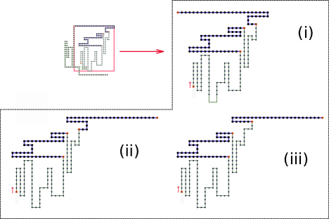
Figure 9. A prudent path obtained by the concatenation of two macro-blocks. We zoom in on the first one, boxed in the rectangle. It has a NE-orientation. In $(\texttt{i})$ we observe that its last block does not achieves the upper exit condition, but it satisfies the lower exit condition. Therefore, in $(\texttt{ii})$ we apply a spatial symmetry to the last block in such a way that it satisfies the upper exit condition. This changes the structure of the last two blocks. In $(\texttt{iii})$ we redefine the last two blocks.

The step will be complete once we show that $\psi_{L}^{3}$ is sub-exponential. To that aim, we need an upper bound on the cardinality of $(\psi_{L}^{3})^{-1}(\Gamma)$ that is uniform on the choice of $\Gamma\in\mathcal{W}_{4,L}$. Thus, we pick $\Gamma\in\mathcal{W}_{4,L}$, say $\Gamma\in\Omega_{n}^{\texttt{NE}}$ with $n\leq L$ and we reconstruct an ancestor $\hat{\Lambda}$ of $\Gamma$ by $\psi_{L}^{3}$. We must first choose $m\leq cL^{1/2}$ the number of macro-blocks in $\hat{\Lambda}$, then choose $\overline{m}$ the number of non empty blocks in $\hat{\Lambda}$. Then, we must choose the indices of those non-empty macro-blocks which gives us $\binom{m}{\overline{m}}$ possibilities and their lengths $l_{i_{1}},\dots,l_{i_{\overline{m}}}$. Once, the latter is done it remains to identify the sequence $(\overline{\Lambda}_{i_{1}},\dots,\overline{\Lambda}_{i_{\overline{m}}})$ (recall 6.16) an we can apply (6.15) to conclude that the total number of ancestors is bounded above by

$$|(\psi_{L}^{3})^{-1}(\Gamma)|\leq\sum_{\overline{m}\leq m\leq cL^{1/2}}\sum_{l_{i_{1}}+\dots+l_{i_{\overline{m}}}=n}\binom{m}{\overline{m}}\prod_{j=1}^{\overline{m}}8l_{i_{j}}$$ (6.18)

and the r.h.s. in (6.18) is smaller than $e^{c_{3}L^{1/2}\log L}$ for some $c_{3}>0$.

Step 4

In this step we conclude our transformation of the prudent path by showing how we concatenate all stretches picked off by the large stretch removing procedure (cf. Step 1) with the rest of the NE-prudent path provided by Steps 1-3. The result will be a NE-prudent path of length $L$.

We pick $\Gamma\in\mathcal{W}_{4,L}$, say $\Gamma\in\Omega_{n}^{\texttt{NE}}$ and we denote by $S_{L-n}$ the west-east block of length $L-n$ that maximizes the energy, i.e, $S_{L-n}$ is made of $(L-n)^{1/2}$ vertical stretches of alternating signs of length $(L-n)^{1/2}-1$ each. Then, the image of $\Gamma$ by $\psi_{L}^{4}$ is obtained by concatenating $S_{L-n}$ with $\Gamma$, i.e.,

$$\psi_{L}^{4}(\Gamma)=S_{L-n}\oplus\Gamma.$$

The image set of $\mathcal{W}_{4,L}$ by $\psi_{L}^{4}$, $\mathcal{W}_{5,L}$, is a subset of $\Omega_{L}^{\texttt{NE}}$ and the number of ancestors of an element in $\Omega_{L}^{\texttt{NE}}$ by $\psi_{L}^{4}$ is clearly less than $L$, which completes the step.

Step 5

We recall that the composition of those maps $\psi_{L}^{4},\dots,\psi_{L}^{1}$ is denoted by $M_{L}$. In this last step we are going to control the energy lost when we apply $M_{L}$ to a given $\omega\in\Omega_{L}^{\texttt{PSAW}}$. We aim at showing that $H\,(\omega)-H\,(M_{L}(\omega))=o(L)$ uniformly on $\omega\in\Omega_{L}^{\texttt{PSAW}}$.

Remark 6.9.

We observe that the image of $\Omega_{L}^{\texttt{PSAW}}$ by $\psi_{L}^{2}\,\circ\,\psi_{L}^{1}$, that is $\mathcal{W}_{3,L}$, contains families of macro-blocks that are a priori not concatenable. For this reason, we recall (6.14) and we define the energy of an element

$$\hat{\Lambda}=(\hat{\Lambda}_{1},\dots,\hat{\Lambda}_{m})\in\Omega_{l_{1}}^{x_{1}}\times\dots\times\Omega_{l_{m}}^{x_{m}}\in\mathcal{W}_{3,L}$$

as the sum of the energies of its macro-blocks, i.e.,

$$H\,(\hat{\Lambda})=\sum_{x=1}^{m}H_{l_{x}}(\hat{\Lambda}_{x}).$$ (6.19)

The sets $\mathcal{W}_{4,L}$ and $\mathcal{W}_{5,L}$, in turn, only contain prudent paths whose energies are well defined by (2.2).

In part (a) of the proof below we will show that the energy lost when applying $\psi_{L}^{2}\,o\,\psi_{L}^{1}$ to a given $\omega\in\Omega_{L}^{\texttt{PSAW}}$ is not larger than $\tilde{L}+c_{1}L^{3/4}$ with $c_{1}>0$ and $\tilde{L}$ the total length of those stretches removed by the large stretch removing procedure. In part (b) we will show that the mapping $\psi_{L}^{3}$ induces at most a loss of energy bounded by $c_{2}L^{3/4}$ with $c_{2}>0$ and finally in part (c) we will observe that the gain of energy associated with $\psi_{L}^{4}$ is $\tilde{L}-\tilde{L}^{1/2}$, which will be sufficient to conclude.

1. We pick $\omega\in\Omega_{L}^{\texttt{PSAW}}$ and we denote by $\Lambda=(\Lambda_{1},\dots,\Lambda_{m})$ its macro-block decomposition. We set $\hat{\Lambda}=(\hat{\Lambda}_{1},\dots,\hat{\Lambda}_{m})=\psi_{L}^{2}\,\circ\,\psi_{L}^{1}(\Lambda)$. Because of the definition of $H\,(\hat{\Lambda})$ in remark 6.9, the interactions between the different macro-blocks of $\Lambda$ do not contribute anymore to the computation of $H\,(\hat{\Lambda})$. The next remark allows us to control the sum of the interactions between different macro-blocks of $\Lambda$.

   Remark 6.10.

   For $j\in\{1,\dots,m\}$, we let $\ell_{1}^{j}$ (resp. $\ell_{2}^{j})$ be the first stretch of the subsequence of odd (resp. even) blocks of $\Lambda_{j}$. Because of the oriented structure of any macro-block, for every $j=2,\dots,m$, it turns out that $\Lambda_{j}$ interacts with $\Lambda_{1}\oplus\dots\oplus\Lambda_{j-1}$ only through $\ell_{1}^{j},\,\ell_{2}^{j}$ and the number of self-touching between $\Lambda_{j}$ and $\Lambda_{1}\oplus\dots\oplus\Lambda_{j-1}$ is bounded from above by $|\ell_{1}^{j}|+|\ell_{2}^{j}|$ (see Figure 5).

   As a consequence of Remark 6.10, the energy provided by the interactions between the different macro-blocks of $\Lambda$ is bounded above by $A_{1}+A_{2}$ with

   $$A_{1} =\sum_{j=1}^{m}\left(\,|\ell_{1}^{j}|\,\mathds{1}_{\big{\{}|\ell_{1}^{j}|\leq L^{1/4}\big{\}}}\,+\,|\ell_{2}^{j}|\,\mathds{1}_{\big{\{}|\ell_{2}^{j}|\leq L^{1/4}\big{\}}}\,\right)$$ (6.20)

   $$A_{2} =\sum_{j=1}^{m}\left(\,|\ell_{1}^{j}|\,\mathds{1}_{\big{\{}|\ell_{1}^{j}|>L^{1/4}\big{\}}}\,+\,|\ell_{2}^{j}|\,\mathds{1}_{\big{\{}|\ell_{2}^{j}|>L^{1/4}\big{\}}}\,\right).$$

   Then, the energy lost during the transformation of $\Lambda$ into $\hat{\Lambda}$ comes on the one hand from the loss of those interactions between macro-blocks and on the other hand from the energy lost inside every macro-blocks due to the large stretch removing procedure. As a consequence, we can write

   $$H\,(\Lambda)-H\,(\hat{\Lambda})\leq A_{1}+A_{2}+\sum_{s=1}^{m}\big{(}\,H(\Lambda_{s})-H(\hat{\Lambda}_{s})\,\big{)},$$ (6.21)

   where we recall that for every $s\in\{1,\dots,m\}$, we have $\hat{\Lambda}_{s}=\mathcal{R}_{t_{s},L}\,\circ\,\mathcal{T}_{t_{s},L}(\Lambda_{s})$ with $t_{s}$ the total length of $\Lambda_{s}$.

   At this stage, for $s\in\{1,\dots,m\}$, we need to bound the energy lost in $\Lambda_{s}$ due to the large stretch removing procedure. We let $\tilde{L}_{s}$ be the total length of those stretches that have been removed and we claim that

   $$H(\Lambda_{s})-H(\hat{\Lambda}_{s})\leq\tilde{L}_{s}-|\ell_{1}^{s}|\,\mathds{1}_{\big{\{}|\ell_{1}^{s}|>L^{1/4}\big{\}}}-|\ell_{2}^{s}|\,\mathds{1}_{\big{\{}|\ell_{2}^{j}|>L^{1/4}\big{\}}}+2L^{1/4}.$$ (6.22)

   To understand (6.22) we must keep in mind that the number of self-touching between two stretches is bounded above by the length of the smallest stretch involved. This implies that, in the odd subsequence of blocks of $\Lambda_{s}$, the number of self-touching between the first and the second stretch is bounded by the length of the second one. Therefore, in the odd subsequence of blocks of $\Lambda_{s}$, the number of self-touching that are lost when applying the last stretch removing procedure is smaller than the sum of all stretches removed in the odd subsequence of oriented blocks minus the length of the very first stretch $\ell_{1}^{s}$, plus the length of the first stretch that has not been removed which, by definition is smaller than $L^{1/4}$. Of course, the same is true for the even subsequence and this explains (6.22).

   At this stage, we combine (6.20  –  6.22) and we use the bound $m\leq cL^{1/2}$ (which implies $A_{1}\leq 2cL^{3/4}$) to conclude that

   $$H\,(\Lambda)-H\,(\hat{\Lambda})\leq\sum_{s=1}^{m}\tilde{L}_{s}+4cL^{3/4}.$$ (6.23)

2. Note that some energy may also be lost in every macro-block during the third transformation described in Section 6.2.3, that is, in the construction of $\psi_{L}^{3}$. Recall (6.16) and the fact that the image of $\hat{\Lambda}$ by $\psi_{L}^{3}$ is denoted by $\overline{\Lambda}$ and has a macro-block decomposition denoted by $(\overline{\Lambda}_{i_{1}},\dots,\overline{\Lambda}_{i_{\overline{m}}})$. Pick $s\in\{1,\dots,\overline{m}\}$ and note that after the first two transformations described in Section 6.2.3, the macro-block $\hat{\Lambda}_{i_{s}}$ has a north-east orientation. In case the very last macro-block of $\hat{\Lambda}_{i_{s}}$ already satisfies the upper exit condition, then the third transformation does nothing and $\hat{\Lambda}_{i_{s}}=\overline{\Lambda}_{i_{s}}$. In case the very last macro-block of $\hat{\Lambda}_{i_{s}}$ satisfies the lower exit condition, we observe that it means necessarily that the large stretch removing procedure has not removed completely the very last block of $\Lambda_{i_{s}}$. Therefore, we apply the third transformation that changes the sign of every stretches in the last block and, if its first stretch is larger than $L^{1/4}$, then the third transformation also changes the sign of the stretches of $\hat{\Lambda}_{i_{s-1}}$ between its last stretch smaller than $L^{1/4}$ and its very last stretch. The existence of such stretch is ensured by the large stretch removing procedure that we applied to the very last block of $\Lambda_{i_{s}}$, as we discussed in. Section 6.2.3. Therefore, by definition, in the third transformation we have lost at most $L^{1/4}$ contacts and consequently

   $$H(\hat{\Lambda})-H(\overline{\Lambda})\leq\sum_{s=1}^{\overline{m}}\big{(}\,H(\hat{\Lambda}_{i_{s}})-H(\overline{\Lambda}_{i_{s}})\,\big{)}\leq\overline{m}L^{1/4}\leq cL^{3/4}.$$ (6.24)

3. With the help of (6.21) and (6.24) above we have proven that for every $\Lambda\in\Omega_{L}^{\texttt{PSAW}}$, by letting $\overline{\Lambda}$ be the image of $\Lambda$ by $\psi_{L}^{3}\,\circ\,\psi_{L}^{2}\,\circ\,\psi_{L}^{1}$, it holds that

   $$H(\Lambda)-H(\overline{\Lambda})\leq\sum_{s=1}^{m}\tilde{L}_{s}+5cL^{3/4}.$$ (6.25)

   For notational convenience we set $\tilde{L}:=\sum_{s=1}^{m}\tilde{L}_{s}$. In Step 4, we have built $M_{L}(\Lambda)$ by concatenating a square block of length $\tilde{L}$ with $\overline{\Lambda}$. The interactions inside the large square block are $\tilde{L}-2\tilde{L}^{1/2}$ and therefore

   $$H(M_{L}(\Lambda))\geq\tilde{L}-2\tilde{L}^{1/2}+H(\overline{\Lambda}).$$ (6.26)

   Finally, (6.25 –  6.26) imply that for every $L\in\mathbb{N}$ and every $\Lambda\in\Omega_{L}^{\texttt{PSAW}}$,

   $$H(\Lambda)-H(M_{L}(\Lambda))\leq 2\tilde{L}^{1/2}+5cL^{3/4}\leq 2L^{1/2}+5cL^{3/4},$$ (6.27)

   and this completes the proof.

7. Proof of Theorem 2.3

We pick $L\in\mathbb{N}$ and we consider $\mathcal{S}_{L}$ the partially directed path that maximizes the self-touching number. We have already seen in Step 4 of Section 6 that $\mathcal{S}_{L}$ is made of $\sqrt{L}-1$ vertical stretches of length $\sqrt{L}$ each and that $H(\mathcal{S}_{L})=L-2\sqrt{L}$. Our proof goes as follows: for every $\epsilon\in(0,1/60)$ we build the set of path $\mathcal{G}_{\epsilon,L}\subset\Omega^{\texttt{ISAW}}_{L}$ such that for every $L$ and $\epsilon$

1. $H(\pi)=H(\mathcal{S}_{L})-13\epsilon L$, for every $\pi\in\mathcal{G}_{\epsilon,L}$,

2. $|\mathcal{G}_{\epsilon,L}|=\binom{L/60}{\epsilon L}.$

As a consequence

$$F^{\texttt{ISAW}}(\beta) :=\liminf_{L\to\infty}\frac{1}{L}\log Z_{\beta,L}^{\texttt{ISAW}}\geq\sup_{\epsilon>0}\bigg{\{}\lim_{L\to\infty}\frac{1}{L}\log\binom{L/60L}{\epsilon L}+\frac{\beta}{L}\big{(}H(\mathcal{S}_{L})-13\epsilon L\big{)}\bigg{\}}$$

$$\geq\beta+\sup_{\epsilon>0}\bigg{\{}\lim_{L\to\infty}\frac{1}{L}\log\binom{L/60}{\epsilon L}-13\,\beta\,\epsilon\bigg{\}},$$ (7.1)

and this completes the proof since the supremum of the r.h.s. in (7) is strictly positive because of our choice of $\epsilon$.

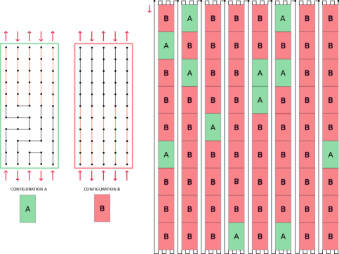
Figure 10. On the left configuration $A$ and $B$ are drawn. The big squared block of size $\sqrt{L}$ on the right is subdivided into $L/60$ rectangular boxes, each of them can be filled with configuration $A$ or $B$ without changing the fact that the resulting path is self-avoiding. The set $\mathcal{G}_{\epsilon,L}$ contains all path obtained by filling $\epsilon L$ boxes with configuration $A$ and the all the others with configuration $B$.
Note, in the picture you have to run over the path by starting on the left top, following the direction given by the arrow. This forces to cross any configuration $A$ and $B$ in a unique way, marked by the arrow on the left side of the picture.

It remains to build the sets $\mathcal{G}_{\epsilon,L}$. First, we partition the collections of $\sqrt{L}-1$ vertical stretches of $\mathcal{S}_{L}$ into groups of $6$ consecutive vertical stretches and then each group is divided vertically into rectangles of heights $10$. This gives us a total of $L/60$ rectangular boxes. On the left hand side of Figure 10 two configurations (denoted by $A$ and $B$) are drawn and each of them is made of $60$ steps. An important feature of configurations $A$ and $B$ is that one can fill every rectangular box with an $A$ or with a $B$ configuration (see the r.h.s. of Figure 10) and still recover a self-avoiding path of size $L$. The $\mathcal{S}_{L}$ path is obtained by filling all boxes with configuration $B$. We also note that filling a box with an $A$ configuration provides exactly $13$ self-touching less than filling the same box with a $B$ configuration.

The set $\mathcal{G}_{\epsilon,L}$ contains all paths obtained by filling the $L/60$ boxes with $\epsilon L$ blocks of type $A$ and $L(\frac{1}{60}-\epsilon)$ blocks of type $B$. Thus, the cardinality of $\mathcal{G}_{\epsilon,L}$ is $\binom{L/60}{\epsilon L}$ and the Hamiltonian of every path in $\mathcal{G}_{\epsilon,L}$ is equal to $H(\mathcal{S}_{L})-13\epsilon L$. This completes the proof.

8. Free Energy: convergence in the right hand side of (2.4)

The goal of this section is to prove the existence of the free energy for the NE-prudent walk. For this purpose, we aim at using a super-additive argument, cf. Proposition A.12 in Giacomin, (2007). It turns out that the sequence $\left(\mathrm{Z}_{\beta,\,L}^{\texttt{NE}}\right)_{L\in\mathbb{N}}$ is not $\log$ super-additive, therefore we introduce a super-additive process, for which the free energy exists, and we show that it rounds up/down $\mathrm{Z}_{\beta,\,L}^{\texttt{NE}}$.

The energy associated with a path is described by an Hamiltonian function $\mathrm{H}\,(w)$, cf. (2.2). We let $\Omega_{L}^{\mathtt{NE},*}\subseteq\Omega_{L}^{\mathtt{NE}}$ be the set of the whole NE-prudent paths for which the upper exit condition is satisfied by all the blocks of the path and we let $\tilde{\Omega}_{L}^{\mathtt{NE},*}\subseteq\Omega_{L}^{\mathtt{NE},*}$ be the set of the $\mathtt{NE}$-prudent paths in $\Omega_{L}^{\mathtt{NE},*}$ for which the first stretch of the path is equal to $0$. We let $\mathrm{Z}_{\beta,\,L}^{\texttt{NE},*}$ and $\tilde{\mathrm{Z}}_{\beta,\,L}^{\texttt{NE},*}$ be the partition functions associated with these sets respectively. In the next lemma we prove that $\tilde{\mathrm{Z}}_{\beta,\,L}^{\texttt{NE},*}$ is $\log$ super-additive.

Lemma 8.1.

The sequence $\left(\tilde{\mathrm{Z}}_{\beta,\,L}^{\texttt{NE},*}\right)_{L\in\mathbb{N}}$ is $\log$ super-additive. As a consequence, the free energy $\tilde{\mathrm{F}}^{\mathtt{NE},*}(\beta)$ exists ant it is finite, i.e.,

$$\tilde{\mathrm{F}}^{\mathtt{NE},*}(\beta):=\lim_{L\to\infty}\frac{1}{L}\log\tilde{\mathrm{Z}}_{\beta,\,L}^{\texttt{NE},*}=\sup_{L\in\mathbb{N}}\frac{1}{L}\log\tilde{\mathrm{Z}}_{\beta,\,L}^{\texttt{NE},*}<\infty.$$

Proof.

We start by showing the super-additivity. We pick $0\leq L^{\prime}\leq L$ and we consider two paths $w_{1}\in\tilde{\Omega}_{L^{\prime}}^{\mathtt{NE},*}$ and $w_{2}\in\tilde{\Omega}_{L-L^{\prime}}^{\mathtt{NE},*}$. We note that we can safely concatenate $w_{1}$ with $w_{2}$, by obtaining the path $w_{1}\oplus w_{2}$, which is an element of $\tilde{\Omega}_{L}^{\mathtt{NE},*}$. Moreover, we note that $\mathrm{H}\,(w_{1}\oplus w_{2})\geq\mathrm{H}_{L^{\prime}}(w_{1})+\mathrm{H}_{L-L^{\prime}}(w_{2})$. We conclude that,

$$\begin{split}&\tilde{\mathrm{Z}}_{\beta,\,L}^{\texttt{NE},*}\geq\sum_{\begin{subarray}{c}w=w_{1}\oplus w_{2}\,:\\ (w_{1},w_{2})\in\tilde{\Omega}_{L^{\prime}}^{\mathtt{NE},*}\times\,\tilde{\Omega}_{L-L^{\prime}}^{\mathtt{NE},*}\end{subarray}}e^{\,\beta\mathrm{H}\,(w)}\geq\sum_{(w_{1},w_{2})\in\tilde{\Omega}_{L^{\prime}}^{\mathtt{NE},*}\times\,\tilde{\Omega}_{L-L^{\prime}}^{\mathtt{NE},*}}e^{\,\beta\mathrm{H}_{L^{\prime}}(w_{1})}e^{\,\beta\mathrm{H}_{L-L^{\prime}}(w_{2})}=\tilde{\mathrm{Z}}_{\beta,\,L^{\prime}}^{\texttt{NE},*}\tilde{\mathrm{Z}}_{\beta,\,L-L^{\prime}}^{\texttt{NE},*}.\end{split}$$ (8.1)

To prove that the limit is finite, we observe that $\mathrm{H}\,(w)\leq L$ and thus $\tilde{\mathrm{Z}}_{\beta,\,L}^{\texttt{NE},*}\leq e^{\beta L}\,|\tilde{\Omega}_{L}^{\mathtt{NE},*}|\leq e^{\beta L}\,|\Omega_{L}^{\mathtt{NE}}|$. This conclude the proof because $\limsup_{L\to\infty}\frac{1}{L}\log|\Omega_{L}^{\mathtt{NE}}|<\infty$. ∎

We are going to compare $\tilde{\mathrm{Z}}_{\beta,\,L}^{\texttt{NE},*}$ with ${\mathrm{Z}}_{\beta,\,L}^{\texttt{NE},*}$, in order to obtain the existence of the free energy for ${\mathrm{Z}}_{\beta,\,L}^{\texttt{NE},*}$. By definition it holds that $\tilde{\mathrm{Z}}_{\beta,\,L}^{\texttt{NE},*}\leq{\mathrm{Z}}_{\beta,\,L}^{\texttt{NE},*}$. On the other hand, we observe that given $w\in\tilde{\Omega}_{L}^{\texttt{NE}}$, if we keep out the first stretch of $w$ (which has $0$ length), then we obtain a path $w^{\prime}\in\Omega_{L-1}^{\texttt{NE}}$. The map which associates $w$ with $w^{\prime}$ is bijective, because there is only one way to add a stretch of $0$ length to a block. Since $\mathrm{H}\,(w)=\mathrm{H}_{L-1}(w^{\prime})$, we conclude that $\tilde{\mathrm{Z}}_{\beta,\,L}^{\texttt{NE},*}\geq{\mathrm{Z}}_{\beta,\,L-1}^{\texttt{NE},*}$. As a consequence, we have that

$$\mathrm{F}^{\mathtt{NE},*}(\beta):=\lim_{L\to\infty}\frac{1}{L}\log{\mathrm{Z}}_{\beta,\,L}^{\texttt{NE},*}\qquad\text{and}\qquad\mathrm{F}^{\mathtt{NE},*}(\beta)=\tilde{\mathrm{F}}^{\mathtt{NE},*}(\beta),\qquad\forall\,\beta\geq 0.$$ (8.2)

We are ready to bound from below and above the function ${\mathrm{Z}}_{\beta,\,L}^{\texttt{NE}}$ by a suitable function for which the free energy exists. We let

$$\Phi_{L,\beta}:=\sum_{L^{\prime}=1}^{L}{\mathrm{Z}}_{\beta,\,L^{\prime}}^{\texttt{NE},*}{\mathrm{Z}}_{\beta,\,L-L^{\prime}}^{\texttt{IPDSAW}}.$$ (8.3)

It is a standard fact, cf.(Giacomin,, 2007, Lemma 1.8) that the existence of the free energy of ${\mathrm{Z}}_{\beta,\,L}^{\texttt{NE},*}$ and ${\mathrm{Z}}_{\beta,\,L}^{\texttt{IDPSAW}}$ implies the existence of the free energy of $\Phi_{L,\beta}$ and

$$\lim_{L\to\infty}\frac{1}{L}\log\Phi_{L,\beta}=\max\Big{\{}F^{\texttt{IPDSAW}}(\beta),F^{\texttt{NE},*}(\beta)\Big{\}}$$ (8.4)

where $\mathrm{F}^{\texttt{IPDSAW}}(\beta)$ is the free energy associated with ${\mathrm{Z}}_{\beta,\,L}^{\texttt{IPDSAW}}$ (its existence was proven in Carmona et al., (2016)).

Proposition 8.2.

It holds that

$$\Phi_{L,\beta}\leq{\mathrm{Z}}_{\beta,\,L}^{\texttt{NE}}\leq e^{o(L)}\Phi_{L,\beta}.$$ (8.5)

As a consequence we have that the free energy of ${\mathrm{Z}}_{\beta,\,L}^{\texttt{NE}}$ exists and it is finite, i.e.,

$$\mathrm{F}^{\mathtt{NE}}(\beta):=\lim_{L\to\infty}\frac{1}{L}\log{\mathrm{Z}}_{\beta,\,L}^{\texttt{NE}}<\infty.$$ (8.6)

Proof.

To prove the lower bound in (8.5) we consider the family of disjoints sets $\Omega_{L^{\prime}}^{\mathtt{NE},*}\times\Omega_{L-L^{\prime}}^{\mathtt{PDSAW}}$, with $L^{\prime}\in\{0,\dots,L\}$. For any $(w^{\prime},w^{\prime\prime})\in\displaystyle\bigcup_{0\leq L^{\prime}\leq L}\Omega_{L^{\prime}}^{\mathtt{NE},*}\times\Omega_{L-L^{\prime}}^{\mathtt{PDSAW}}$. Let $w=w^{\prime}\oplus w^{\prime\prime}$ be the concatenation of $w^{\prime\prime}$ with $w^{\prime}$. Since $\mathrm{H}_{N}(w)\geq\mathrm{H}_{L^{\prime}}(w^{\prime})+\mathrm{H}_{L-L^{\prime}}(w^{\prime\prime})$ we have

$$\mathrm{Z}_{L,\beta}^{\mathtt{NE}}:=\sum_{w\in\Omega_{L}^{\texttt{NE}}}e^{\,\beta\mathrm{H}\,(w)}\geq\sum_{L^{\prime}=0}^{L}\sum_{\begin{subarray}{c}w\in\Omega_{L}^{\texttt{NE}}\,:\\ w=w^{\prime}\oplus w^{\prime\prime},\\ (w^{\prime},w^{\prime\prime})\in\Omega_{L^{\prime}}^{\mathtt{NE},*}\times\Omega_{L-L^{\prime}}^{\mathtt{PDSAW}}\end{subarray}}e^{\,\beta\mathrm{H}\,(w)}$$

$$\qquad\geq\sum_{L^{\prime}=0}^{L}\sum_{\begin{subarray}{c}w\in\Omega_{L}^{\texttt{NE}}\,:\\ w=w^{\prime}\oplus w^{\prime\prime},\\ (w^{\prime},w^{\prime\prime})\in\Omega_{L^{\prime}}^{\mathtt{NE},*}\times\Omega_{L-L^{\prime}}^{\mathtt{PDSAW}}\end{subarray}}e^{\,\beta(\mathrm{H}\,(w^{\prime})+\mathrm{H}\,(w^{\prime}))}=\sum_{L^{\prime}=1}^{L}{\mathrm{Z}}_{\beta,\,L^{\prime}}^{\texttt{NE},*}{\mathrm{Z}}_{\beta,\,L-L^{\prime}}^{\texttt{IPSAW}}.$$

The strategy to prove the upper bound in (8.5) is similar to the strategy used for the proof of Theorem 2.1 in Section 6. To be more precise, we associate with each $w\in\Omega_{L}^{\mathtt{NE}}$ two paths $u^{\prime}\in\Omega_{L^{\prime}}^{\mathtt{NE},*}$ and $w^{\prime}\in\Omega_{L-L^{\prime}}^{\mathtt{PDSAW}}$, for some $0<L^{\prime}<L$, with $L^{\prime}=L^{\prime}(w)$, through a sub-exponential function (cf. Definition 6.1). We let $(\pi_{1},\dots,\pi_{r})$ be the block decomposition of $w$. We consider the last block $\pi_{r}$, of length $L-L^{\prime}$, for some $L^{\prime}<L$. We apply the large stretch removing procedure to $\pi_{r}$, i.e., by starting from the first stretch, we pick off all the consecutive stretches larger than $L^{1/4}$ in the block $\pi_{r}$. Let $\pi_{r}^{\prime}$ be the result of this operation. Let $\tilde{L}$ be the total length of the stretches that we picked off. We define an oriented block made of $\sqrt{\tilde{L}}$ vertical stretches of alternating sings of length $\sqrt{\tilde{L}}-1$. This configuration maximizes the energy of a block of length $\tilde{L}$. The orientation of this block is the same as that of $\pi_{r}$. We concatenate this block with $\pi_{r}^{\prime}$ and we call $w^{\prime}$ the path obtained at the end of this operation. By construction $w^{\prime}\in\Omega_{L-L^{\prime}}^{\mathtt{PDSAW}}$. We let $u^{\prime}:=\pi_{1}\oplus\dots\oplus\pi_{r-1}$, so that $(u^{\prime},w^{\prime})\in\Omega_{L^{\prime}}^{\mathtt{NE},*}\times\Omega_{L-L^{\prime}}^{\mathtt{PDSAW}}$. The computations we did in Steps $1-4$ in Section 6 ensure that the function which associates $w$ with $(u^{\prime},w^{\prime})$ is sub-exponential and, by reasoning as in Step $5$ of Section 6, it turns out that $H\,(w)-\big{(}H_{L^{\prime}}(u^{\prime})+H_{L-L^{\prime}}(w^{\prime})\big{)}\leq o(L)$, uniformly on $w\in\Omega_{L}^{\texttt{NE}}$. This suffices to conclude the proof.

∎

References

- Beaton and Iliev, (2015) Beaton, N. and Iliev, G. (2015). Two-sided prudent walks: a solvable non-directed model of polymer adsorption. J. Stat. Mech. Theory Exp., (9):P09014, 23.
- Beffara et al., (2010) Beffara, V., Friedli, S., and Velenik, Y. (2010). Scaling limit of the prudent walk. Electronic Communications in Probability, 15:44–58.
- Bousquet-Mélou, (2010) Bousquet-Mélou, M. (2010). Families of prudent self-avoiding walks. Journal of combinatorial theory series a, 117(3):313 – 344.
- Brak et al., (1992) Brak, R., Guttman, A., and Whittington, S. (1992). A collapse transition in a directed walk model. J. Phys. A: Math. Gen., 25:2437–2446.
- Carmona et al., (2016) Carmona, P., Nguyen, G. B., and Pétrélis, N. (2016). Interacting partially directed self avoiding walk. from phase transition to the geometry of the collapsed phase. Ann. Probab, 9(5):3234–3290.
- Carmona and Pétrélis, (2016) Carmona, P. and Pétrélis, N. (2016). Interacting partially directed self avoiding walk: scaling limits. Electron. J. Probab., 21:52 pp.
- den Hollander, (2009) den Hollander, F. (2009). Random polymers, volume 1974 of Lecture Notes in Mathematics. Springer-Verlag, Berlin. Lectures from the 37th Probability Summer School held in Saint-Flour, 2007.
- Dethridge and Guttmann, (2008) Dethridge, J. and Guttmann, A. (2008). Prudent self-avoiding walks. Entropy, 10(3):309–318.
- Giacomin, (2007) Giacomin, G. (2007). Random Polymer Models. Imperial College Press, World Scientific.
- Nguyen and Pétrélis, (2013) Nguyen, G. B. and Pétrélis, N. (2013). A variational formula for the free energy of the polymer collapse. J. Stat. Phys., 151(6):1099–1120.
- Saleur, (1986) Saleur, H. (1986). Collapse of two-dimensional linear polymers. Journal of Statistical Physics, 45(3):419–438.
- (12) Tesi, M. C., Janse van Rensburg, E. J., Orlandini, E., and Whittington, S. G. (1996a). Monte carlo study of the interacting self-avoiding walk model in three dimensions. Journal of Statistical Physics, 82(1):155–181.
- (13) Tesi, M. C., van Rensburg, E. J. J., Orlandini, E., and Whittington, S. G. (1996b). Interacting self-avoiding walks and polygons in three dimensions. Journal of Physics A: Mathematical and General, 29(10):2451.
- van der Hofstad and A.Klenke, (2001) van der Hofstad, R. and A.Klenke (2001). Self-attractive random polymers. Ann. Appl. Probab., 11(4):1079–1115.
- van der Hofstad et al., (2002) van der Hofstad, R., Klenke, A., and König, W. (2002). The critical attractive random polymer in dimension one. J. Statist. Phys., 106(3-4):477–520.
- Zwanzig and Lauritzen, (1968) Zwanzig, R. and Lauritzen, J. I. (1968). Exact calculation of the partition function for a model of two dimensional polymer crystallization by chain folding. J. Chem. Phys., 48(8):3351–3360.