Quadratically damped oscillators with non-linear restoring force

Abstract

In this paper we qualitatively analyse quadratically damped oscillators with non-linear restoring force. In particular, we obtain Hamiltonian structure and analytical form of the energy functions.

1 Introduction

Modelling of physical systems is one of the key goals of mathematical physics. Physical systems, in reality, are not ideal and systems like, the harmonic oscillator and the viscously damped oscillators are actually idealisations of real life systems. Real life systems are generally non-linear in character and are usually represented by a variety of different mathematical descriptions. To model the phenomenon of damping, specially at higher velocities it is necessary to introduce a quadratic non-linearity and the corresponding term is in general of the form - $sgn(\dot{x})\dot{x}^{2}$ [16, 20]. In recent times, such systems have gained much attention because of vast range of applications in engineering, specially in the problems involving hydrological drag and aerodynamics [22, 14].

In [11], Kovacic and Rakaric have considered a system where the quadratic damping coefficient is a constant and with a non-linear forcing term of the form, $F(x)=sgn(x)|x|^{\alpha}$, where $\alpha$ is positive real constant. For linear, i.e, viscous, damping the systems can easily be solved using standard well established mathematical techniques. However, with quadratic damping the complexity in solving such problems using analytic methods increases. In the case of quadratic damping with non-linear forcing term $F(x)$ the orbits involve discontinuous jumps at every quadrant boundary. To exactly solve such systems is not easy as four different systems have to be solved for each quadrant and their solutions need to be matched at the respective boundaries. Numerical approaches are, therefore, necessary to deal with such systems as they provide valuable insights of the qualitative nature of the system.

Quadratic damping arise generally in flows with high flow velocity. In general, the drag force consists of linear as well as quadratic terms. For slow flows, the linear term dominates and at higher velocity the linear term becomes negligible and quadratic term dictates the motion. In fluid dynamics, Morison’s equation is one of the fundamental equations which gives the net in-line force on a fixed body in oscillatory flows. It is a semi-empirical equation and is given as

$$F=a\dot{v}+bv|v|.$$ (1.1)

Here $a$ and $b$ are proportionality constants which depend upon the density and the geometry of the body and $v(t)$ is the flow velocity. The first term is the inertial force and the second term gives the drag force on the object. In [22], Yamamoto and Nath studied the oscillatory flows around a cylinder and they determined the drag force as being directly proportional to the signed velocity squared where the coefficients were determined experimentally. In [14], Madison used a quadratic damping force caused by fluid friction to study isenthalpic oscillations in a saturated two-phase fluid.

In this work, we consider a general system,

$$x^{\prime\prime}+sgn(x^{\prime})f(x)x^{\prime 2}+sgn(x)|g(x)|=0,$$ (1.2)

where the damping coefficient is a function of the displacement and study it for different cases using different instances of $f(x)$ and $g(x)$. We formulate a generalised scheme for the calculation of the mechanical energy given by a undamped oscillator. We also derive Hamiltonian description for the system which is basically piecewise in different quadrants.

The organisation of the paper is as follows. In section 2, we transform the second-order differential equation (1.2) into a first-order differential equation for the kinetic energy of the corresponding undamped oscillator. Further we give the Hamiltonian structure for the system. To analyse the system, we consider the specific cases of odd and even forcing terms and provide some illustrative examples. Finally analytic expressions are calculated for the energy and the Hamiltonians.

2 Oscillators with non-negative real-power restoring force and quadratic damping.

Oscillators with quadratic damping together with non-linear non-negative real-power restoring force are interesting problems and were well studied by I. Kovacic and Z. Rakaric in [11], they consider a second-order differential equation of the form

$$x^{\prime\prime}+\mu\,sgn(x^{\prime})x^{\prime 2}+sgn(x)|x|^{\alpha}=0,$$ (2.1)

where the prime denotes differentiation with respect to $t$, $\mu$ denotes the damping coefficient and $\alpha\in\mathbb{R}^{+}$. We study the above system in a more general setting with displacement dependent damping so that $\mu=f(x)$, and with a forcing term $sgn(x)|g(x)|$. The corresponding equation is then given by

$$x^{\prime\prime}+sgn(x^{\prime})f(x)x^{\prime 2}+sgn(x)|g(x)|=0.$$ (2.2)

From (2.2) we have

$$\frac{d}{dt}\left[\frac{1}{2}(x^{\prime})^{2}+\int_{0}^{x}|g(s)|\,ds\right]=-sgn(x^{\prime})f(x)x^{\prime 3}.$$ (2.3)

Let $T=\frac{1}{2}(x^{\prime})^{2}$, and,$V=\int_{0}^{x}|g(s)|\,ds$, then $E=T+V$. Now, from (2.3) we can have

$$\frac{dT}{dx}+2\,sgn(x^{\prime})f(x)\,T=-sgn(x)|g(x)|.$$ (2.4)

In order to understand the qualitative features of the system we consider the following two cases depending on the whether the forcing term is even or odd.

Case 1: odd-power restoring forces

In this situation (2.2) can be written as

$$x^{\prime\prime}+sgn(x^{\prime})f(x)x^{\prime 2}+g(x)=0,$$ (2.5)

which is the same system considered in [18]. As shown in [18] for even damping coefficient, we have a damped orbit (fig(1b)) and for odd damping we have a closed orbit (fig(1a)).

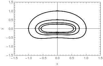
(a) $f(x)=x,\,\,g(x)=x^{3}$.

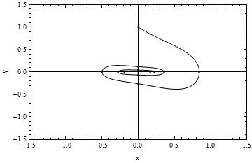
(b) $f(x)=1,\,\,g(x)=x^{3}$.

Figure 1: For odd-power restoring force with odd (a) and even (b) damping coefficients.

As an example when $f(x)=1,\,g(x)=x^{3}$, the system is given as

$$x^{\prime\prime}+sgn(x^{\prime})x^{\prime 2}+x^{3}=0\,$$

Then from (2.4) we have

$$\frac{dT}{dx}+2T=-x^{3}\,\,\,\,\,\,x^{\prime}>0,$$

$$\frac{dT}{dx}-2T=-x^{3}\,\,\,\,\,\,x^{\prime}<0.$$

Solution to the above equations are given as

$$T=\frac{1}{8}\left(3-6x+6x^{2}-4x^{3}\right)+c_{+}\,e^{-2x}\,\,\,\,\,x^{\prime}>0,$$

$$T=\frac{1}{8}\left(3+6x+6x^{2}+4x^{3}\right)+c_{-}\,e^{2x}\,\,\,\,\,x^{\prime}<0,$$

where $c_{\pm}$ are constants of integration and are fixed using the initial conditions. The corresponding energies are

$$E=T+V=\frac{1}{8}\left(3-6x+6x^{2}-4x^{3}\right)+c_{+}\,e^{-2x}+\frac{x^{4}}{4},\,\,\,\,x^{\prime}>0,$$

$$E=T+V=\frac{1}{8}\left(3+6x+6x^{2}+4x^{3}\right)+c_{-}\,e^{2x}+\frac{x^{4}}{4},\,\,\,\,x^{\prime}<0.$$

Now consider another example with odd damping coefficient, $f(x)=x$. In this setting, (2.5) becomes

$$x^{\prime\prime}+sgn(x^{\prime})xx^{\prime 2}+x^{3}=0\,$$

and (2.4) takes the form

$$\frac{dT}{dx}+2xT=-x^{3}\,\,\,\,\,\,x^{\prime}>0,$$

$$\frac{dT}{dx}-2xT=-x^{3}\,\,\,\,\,\,x^{\prime}<0.$$

The final energy is given as

$$E=T+V=\frac{1}{2}\left(1-x^{2}\right)+c_{+}\,e^{-x^{2}}+\frac{x^{4}}{4},\,\,\,\,x^{\prime}>0,$$

$$E=T+V=\frac{1}{2}\left(1+x^{2}\right)+c_{-}\,e^{x^{2}}+\frac{x^{4}}{4},\,\,\,\,x^{\prime}<0,$$

where $c_{\pm}$ are constants of integration. Figure (2a, 2b) shows the energy-displacement curve for the above considered examples, and the corresponding phase space orbits are shown in figure (1a, 1b).

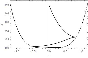
(a) $f(x)=1,\,g(x)=x^{3}$.

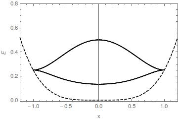
(b) $f(x)=x,\,g(x)=x^{3}$.

Figure 2: Energy variation with displacement for odd-power restoring forces.

Case 2: even-power restoring forces

In the case of even-power restoring force, the forcing term is again an odd function and behaves qualitatively in the same manner as in the odd-power case. However, the damping and the period will vary depending upon $\alpha$. Figure(3) shows the orbits for even and odd damping coefficients.

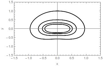
(a) $f(x)=x,\,\,g(x)=x^{2}$.

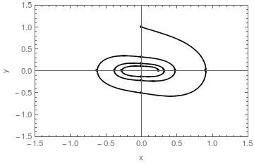
(b) $f(x)=1,\,\,g(x)=x^{2}$.

Figure 3: Even-power restoring with odd (a) and even (b) damping.

The equations for this case are given as

$$x^{\prime\prime}+sgn(x^{\prime})f(x)x^{\prime 2}+g(x)=0,\,\,\,\,\,\,x<0,$$

$$x^{\prime\prime}+sgn(x^{\prime})f(x)x^{\prime 2}-g(x)=0,\,\,\,\,\,\,x<0.$$

The dynamics in this case varies in each quadrants of the phase plane. To illustrate this case, consider an example with $f(x)=1,\,g(x)=x^{2}$. The system is given as

$$x^{\prime\prime}+sgn(x^{\prime})x^{\prime 2}+sign(x)x^{2}=0.\,$$

The dependence of energy on displacement can be computed using (2.4) and $E=T+V$ and leads to the following expressions

$$E=\frac{1}{4}\left(-1+2x-2x^{2}\right)+c_{++}e^{-2x}+\frac{x^{3}}{3},\,\,\,\,\,x>0,\,x^{\prime}>0$$

$$E=\frac{1}{4}\left(1+2x+2x^{2}\right)+c_{-+}e^{2x}+\frac{x^{3}}{3},\,\,\,\,\,x<0,\,x^{\prime}>0$$

$$E=\frac{1}{4}\left(1-2x+2x^{2}\right)+c_{+-}e^{-2x}+\left|\frac{x^{3}}{3}\right|,\,\,\,\,\,x>0,\,x^{\prime}<0$$

$$E=\frac{1}{4}\left(-1-2x-2x^{2}\right)+c_{--}e^{2x}+\left|\frac{x^{3}}{3}\right|,\,\,\,\,\,x<0,\,x^{\prime}<0$$

where $c_{\pm\pm}$ are constants of integration. Figure (4a) shows the energy variation with displacement with the dotted lines denoting the potential $V$.

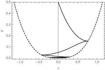
(a) $f(x)=1,\,g(x)=x^{2}$.

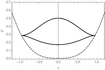
(b) $f(x)=x,\,g(x)=x^{2}$.

Figure 4: Energy-displacement curve for even and odd damping functions.

For an example with closed orbits, assume $f(x)=x$. The system is given as

$$x^{\prime\prime}+sgn(x^{\prime})xx^{\prime 2}+sign(x)x^{2}=0.\,$$

By following a similar procedure as outlined before we find the energy dependence on displacement to be given by

$$E=e^{-x^{2}}\left(-\frac{1}{2}e^{x^{2}}x+\frac{1}{4}\sqrt{\pi}\mathcal{E}rfi(x)\right)+c_{++}e^{-x^{2}}+\frac{x^{3}}{3},\,\,\,\,\,x>0,\,x^{\prime}>0$$

$$E=e^{x^{2}}\left(\frac{1}{2}e^{-x^{2}}x-\frac{1}{4}\sqrt{\pi}\mathcal{E}rf(x)\right)+c_{-+}e^{x^{2}}+\frac{x^{3}}{3},\,\,\,\,\,x<0,\,x^{\prime}>0$$

$$E=e^{-x^{2}}\left(\frac{1}{2}e^{x^{2}}x-\frac{1}{4}\sqrt{\pi}\mathcal{E}rfi(x)\right)+c_{+-}e^{-x^{2}}+\left|\frac{x^{3}}{3}\right|,\,\,\,\,\,x>0,\,x^{\prime}<0$$

$$E=e^{x^{2}}\left(-\frac{1}{2}e^{-x^{2}}x+\frac{1}{4}\sqrt{\pi}\mathcal{E}rf(x)\right)+c_{--}e^{x^{2}}+\left|\frac{x^{3}}{3}\right|,\,\,\,\,\,x<0,\,x^{\prime}<0$$

where $c_{\pm\pm}$ are constants of integration and $\mathcal{E}rf\,and\,\mathcal{E}rfi$ are error functions and imaginary error functions. Figure (4b) shows the energy variation with displacement with dotted lines denoting potential $V$.

2.1 The Hamiltonian structure of the system

In the above analysis the mechanical energy $E=T+V$ corresponds to that of a particle of unit mass moving in the potential $V$. Owing to the presence of the damping term it is quite natural that the mechanical energy is not conserved. However, it is interesting to note that in the case of ODEs of the form of (1.2) one can formulate an alternative description in terms of a variable mass. In the following we consider first a second-order ODE with a quadratic dependence on the velocity given by

$$\ddot{x}+f(x)\dot{x}^{2}+g(x)=0.$$ (2.5)

we assume $f(x)$ and $g(x)$ are such that $f(0)=g(0)=0$ and $f(x)$ is integrable while $g^{\prime}(0)>0$. The functional form of $g(x)=g^{\prime}(0)x+g_{n}(x)$ where $g_{n}(x)$ is analytic. As demonstrated in [15, 17], the Jacobi Last Multiplier (JLM) provides a convenient tool for obtaining a Lagrangian for second-order equations of the form $\ddot{x}=\mathcal{F}(x,\dot{x})$. It is defined as a solution of

$$\frac{d}{dt}\log M+\frac{\partial\mathcal{F}(x,\dot{x})}{\partial\dot{x}}=0.$$ (2.6)

In the present case it follows that

$$M=\exp\left(2F(x)\right),\;\;\;\;\hbox{ where }\;\;\;\;F(x)=\int_{0}^{x}f(s)ds.$$ (2.7)

The relationship between the JLM, $M$ and the Lagrangian is provided by $M=\partial^{2}L/\partial\dot{x}^{2}$ as a consequence of which for (2.5) the Lagrangian may be expressed in the form

$$L=\frac{1}{2}e^{2F(x)}\dot{x}^{2}-V(x),$$ (2.8)

where $V(x)$ is determined by substituting (2.8) into the Euler-Lagrange equation

$$\frac{d}{dt}\left(\frac{\partial L}{\partial\dot{x}}\right)=\left(\frac{\partial L}{\partial x}\right),$$

which immediately gives

$$V(x)=\int_{0}^{x}e^{2F(s)}g(s)ds.$$ (2.9)

By means of the standard Legendre transformation we can obtain the Hamiltonian as

$$H=\frac{1}{2}e^{2F(x)}\dot{x}^{2}+\int_{0}^{x}e^{2F(s)}g(s)ds.$$ (2.10)

It is easily verified that the Hamiltonian is a constant of motion and the expression for the conjugate momentum $p=e^{2F(x)}\dot{x}$ suggests that $M=e^{2F(x)}$ serves as a position dependent mass term. In fact equations with quadratic velocity dependance of the type considered here naturally arise in the Newtonian formulation of the equation of motion of a particle with a variable mass. Clearly then, the trajectories for arbitrary intial condition $(x_{0},y_{0})$ where $y=\dot{x}$ are given by

$$\frac{1}{2}e^{2F(x)}y^{2}+V(x)=\frac{1}{2}e^{2F(x)}y_{0}^{2}+V(x_{0}).$$ (2.11)

In terms of the canonical momentum, $p=e^{2F(x)}\dot{x}$, the Hamiltonian $H$ becomes

$$H=\frac{p^{2}}{2e^{2F(x)}}+V(x).$$ (2.12)

From the above it is obvious that in the case of oscillators with quadratic damping and normal non-linear forcing terms, the Hamiltonian for system (2.1) is given by

$$H^{\pm\pm}=\frac{1}{2}e^{\pm 2F(x)}x^{\prime 2}\pm\int_{0}^{x}e^{\pm 2F(s)}g(s)\,ds,$$ (2.13)

where $F(x)=\int_{0}^{x}f(s)\,ds$ and the first $(\pm)$ in the superscript of $H$ denotes $(\pm)$ in the power of exponential which basically comes from sign function in the coefficient of damping term while the second one denotes $(\pm)$ in the forcing term. It is also natural to define the potential function by

$$V_{H}^{\pm}=\int_{0}^{x}e^{\pm 2F(s)}g(s)\,ds.$$ (2.14)

In the following we provide explicit expressions for the Hamiltonian for our previous examples and also list the comparative changes in the values of $H$ and $E$ for each case. The Hamiltonian for the above examples are given as

$example\,:\,f(x)=1,\,g(x)=x^{3}$

$$H^{\pm}=\frac{1}{2}e^{\pm 2x}x^{\prime 2}+\frac{(3+e^{\pm 2x}\left(-3\pm 2x\,(3\pm x(-3\pm 2x)))\right)}{8},$$

$example\,:\,f(x)=x,\,g(x)=x^{3}$

$$H^{\pm}=\frac{1}{2}e^{\pm x^{2}}x^{\prime 2}+\frac{\left(1+e^{\pm x^{2}}(-1+\pm x^{2})\right)}{2}.$$

The above Hamiltonians do not depend on the sign of displacement. This is evident from (2.5). Table (1) shows the changes in the values of the Hamiltonian and energy $E$ in each complete cycle.

$n^{th}$ cycle	$\Delta H$	$\Delta E$
1	-0.493039	-0.493039
2	-0.00603154	-0.00603154
3	-0.000307447	-0.000684351
4	-0.0000497198	-0.000154833

Table 1: Change in Hamiltonian and Energy in each full cycle.

The Hamiltonian for the examples in even-power case are given as

$$H^{s\,w}=\frac{1}{2}e^{s\,x^{2}}x^{\prime 2}+\frac{w\left(2e^{s\,x^{2}}\sqrt{s}x-\sqrt{\pi}\mathcal{E}rfi(\sqrt{s}x)\right)}{4s^{3/2}},$$

where $s,\,w=\{\pm 1\}$ and denotes the sign of displacement $x$ and velocity $x^{\prime}$, respectively. Table (2) shows the change in the values of Hamiltonian and energy in each cycle.

$n^{th}$ cycle	$\Delta H$	$\Delta E$
1	-0.486074	-0.486074
2	-0.011064	-0.0278193
3	-0.000956281	-0.000956281
4	-0.000216832	-0.000714582

Table 2: Change in Hamiltonian and energy in each complete cycle.

3 Conclusion

In this paper, a general quadratically damped oscillator with non-linear force is studied. The associated energy, taken as energy of an undamped oscillator, has been calculated and an analytic expression for the same is obtained. Hamiltonian description of the system is shown and analytic expression has been obtained for different instances.

References

- [1] A. Chiellini, Sull’integrazione dell’equazione differenziale , Bollettino dell’Unione Matematica Italiana, 10, 301-307 (1931).
- [2] R.M. Corless, G. H. Gonnet, D. E. G. Hare, D. J. Jeffrey, and D. E. Knuth, On the Lambert W function. Advances Computational Maths 5 (1996), 329-359.
- [3] L. Cveticanin, Oscillator with strong quadratic damping force, Publ. Inst. Math. (Beograd) (N.S.) 85(99) (2009), 119–130.
- [4] L. Cveticanin, Analysis techniques for the various forms of the Duffing equation in The Duffing Equation: Nonlinear Oscillators and their Behaviour, 81–137, Ed. I. Kovacic and M. J. Brennan, Wiley, Chichester, 2011.
- [5] T. H. Fay, Quadratic damping. Internat. J. Math. Ed. Sci. Tech. 43 (2012), no. 6, 789-803.
- [6] A. Ghose Choudhury and P. Guha, On isochronous cases of the Cherkas system and Jacobi’s last multiplier, J. Phys. A: Math. Theor. 43 (2010) 125202.
- [7] A. Ghose Choudhury and P. Guha, An analytic technique for the solutions of nonlinear oscillators with damping using the Abel Equation, to appear in Discontinuity, Nonlinearity and Complexity.
- [8] P. Guha and A. Ghose Choudhury, The Jacobi last multiplier and isochronicity of Liénard type systems, Rev. Math. Phys. 25 (6) (2013) 1330009.
- [9] T. Harko, F. S. N. Lobo, M. K. Mak, A Chiellini type integrability condition for the generalized first kind Abel differential equation, Universal Journal of Applied Mathematics, 1 (2013) 101-104.
- [10] K. Klotter, Free oscillations of systems having quadratic damping and arbitrary restoring forces. J. Appl. Mech. 22 (1955), 493-499.
- [11] I. Kovacic and Z. Rakaric, Study of oscillators with a non-negative real-power restoring force and quadratic damping. Nonlinear Dynam. 64 (2011), no. 3, 293-304.
- [12] J.H.Lambert, Acta Helvitica 3 (1758) 128-168.
- [13] A. Liénard, Revue générale de l’électricité 23, 901- 912, and 946-954 (1928).
- [14] J.V. Madison, Isenthalpic oscillations with quadratic damping in saturated two-phase fluids, WIT Transactions on Engineering Sciences, Vol 74, doi: 10.2495/AFM120351.
- [15] M.C.Nucci and P.G.L.Leach, The Jacobi’s Last Multiplier and its applications in mechanics, J. Phys. Scr. 78(2008) 065011.
- [16] A. H. Nayfeh and D. Mook, Nonlinear Oscillations, Wiley, New York, 1979.
- [17] M.C. Nucci and K.M. Tamizhmani, Lagrangians for dissipative nonlinear oscillators: the method of Jacobi last multiplier, Journal of Nonlinear Mathematical Physics, Vol. 17, No. 2 (2010) 167178.
- [18] A. Pandey, A. Ghose Choudhury and P. Guha, Cheillini integrability and quadratically damped oscillators, arXiv:1608.07377 [nlin.SI].
- [19] A. D. Polyanin and V. F. Zaitsev, Handbook of Exact Solutions for Ordinary Differential Equations, Chapman & Hall/CRC, Boca Raton, London, New York, Washington, D. C. (2003).
- [20] Ruzicka, J.E. Derby, T.E.: Influence of Damping in Vibration Isolation. T.S.a.V.I. Centre, US Department of Defence, Washington (1971).
- [21] M Sabatini, On the period Function of Liénard Systems, J. Diff. Eqns. 152,467-487, (1999).
- [22] Yamamoto, T., and Nath, J. (2011). High Reynolds Number Oscillating Flow By Cylinders, Coastal Engineering Proceedings, 1(15). doi:http://dx.doi.org/10.9753/icce.v15.