Reduced density matrix and order parameters of a topological insulator

Abstract

It has been recently proposed that the reduced density matrix may be used to derive the order parameter of a condensed matter system. Here we propose order parameters for the phases of a topological insulator, specifically a spinless Su-Schrieffer-Heeger (SSH) model, and consider the effect of short-range interactions. All the derived order parameters and their possible corresponding quantum phases are verified by the entanglement entropy and electronic configuration analysis results. The order parameter appropriate to the topological regions is further proved by calculating the Berry phase under twisted boundary conditions. It is found that the topological non-trivial phase is robust to the introduction of repulsive inter-site interactions, and can appear in the topological trivial parameter region when appropriate interactions are added.

I Introduction

At absolute zero temperature, a quantum many-body system can undergo a quantum phase transition (QPT) Sachdev2000 ; Carr2011 by varying a non-thermal external driving parameter such as the magnetic field. Across the quantum critical point, the qualitative structure of the many-body ground state wavefunction undergoes a significant change and the change is completely driven by the quantum fluctuation in the ground state. To characterize a continuous quantum phase transition, a traditional approach is to use Landau’s symmetry breaking theory in which the order parameter plays the central role. The order parameter is nonzero in the symmetry broken phase while it vanishes in other phases. Through the emergency of the order parameter, the phase boundary can also be determined. However, to find an appropriate order parameter describing certain phase is a non-trivial task. People have to rely on physical intuition or resort to methods such as group theory and the renormalization group analysis. A prior knowledge of the symmetry breaking of the system is required and the methods are not always guaranteed to apply, especially to systems exhibiting topological QPTs Wen2004 .

On the other hand, in the recent decade much attention has been paid to investigate quantum phase transitions from the perspective of quantum information science. One of the examples is the study of quantum entanglement in quantum critical phenomena Amico2008 ; Osborne2002 ; Osterloh2002 . Being a measure of quantum correlation, it is believed that the entanglement plays a crucial role in QPTs. Studies showed that the quantum entanglement helps to witness quantum critical points and exhibits interesting properties such as scaling Osborne2002 ; Osterloh2002 , singularity or maximum GuEE , etc., in various transitions. It was also shown to be capable of detecting topological orders Levin2006 ; Kitaev2006 . In contrast to the traditional approach, the application of the quantum entanglement does not require a prior knowledge of the system’s symmetry and this makes it a great advantage to use for the study of QPTs.

Recently, along the streamline of quantum entanglement, Gu, Yu and Lin Gu2013 proposed a systematic way to derive the order parameter by studying mutual information and the spectra of the corresponding reduced density matrix. To apply the scheme, one only needs the knowledge of the ground state of the system but not the symmetries existing in it. By studying the single site and two sites reduced density matrices, the order parameters for the spin-density wave (SDW), charge-density wave (CDW), bond-order wave (BOW) and the phase separation phase (PS) in the one-dimensional extended Hubbard model were successfully obtained YU2016 . Meanwhile, there are other independent proposals to derive the order parameter. Furukawa, Misguich, and Oshikawa Furukawa2006 proposed a variational method by investigating a set of low-energy “quasi-degenerate” states that lead to the symmetry breaking in the thermodynamic limit. Their scheme was later improved by Henley and Changlani Henley2014 . Cheong and Henley Cheong2009 on the other hand suggested to study the singular-value decomposition of the correlation density matrix to gain information on the correlation function and the order parameter. Compared to those methods, the one proposed by Gu et al.Gu2013 is a non-variational approach and is relatively more intuitive to apply. Moreover, it also establishes a connection between the mutual information and the order parameters.

In this work, we apply Gu et al.’s method to a problem which has topological properties. The model considered is a one-dimensional spinless fermions Su-Schrieffer-Heeger (SSH)-like model with explicit dimerization. The original SSH model ssh describes the coupling between spinfull electrons and phonons and was proposed to describe the one-dimensional conducting polyacetylene; the condensation of the phonons leads to a dimerization of the lattice. The simplified model considered here, with explicit dimerization, can be viewed as a two-band model where interband hopping with alternating amplitudes takes place at the same site or neighboring sites. The model has two gapped phases, depending on the relative amplitudes of the two sets of hoppings. If the two sets of hoppings are equal (no dimerization), the spectrum is gapless. One of the phases is topologically trivial while the other has a nonvanishing winding number and fermionic edge states. The model has no true topological order but is a symmetry-protected topological system hasan ; szhang ; schnyder . The model is also related to Shockley’s model (see for instance yakovenko ). We identify the order parameters appropriate to describe the two phases: in the trivial phase the order parameter is fully local and involves the two bands at a given site. In the topological phase the order parameter involves two neighboring lattice sites.

The effect of interactions is also addressed. Both the separate addition of dimerization and interactions lead to spectra that are gapped. In the case of spinless fermions Pauli’s principle forbids a Hubbard-like term and a nearest-neighbor interaction term is the dominant. Dimerization and the consequent existence of two bands allows a local interband Hubbard term. These various cases have been extensively studied before using various techniques such as bosonization and the density matrix renormalization group method (DMRG)white . The addition of interactions to the problem leads to a competition between various orderings. In the case of spinfull systems there is a competition between bond-ordered, charge density waves and spin density waves wang ; jeckelmann ; riera ; zhang1 as a result of the phonon and electronic repulsion terms. The competition in the case of explicit dimerization has also been addressed benthien as well as the contribution of bond-bond and mixed bond-site electronic couplings campbell . These competitions continue to attract interest in the literature (see for instance, ejima ; kumar ; weber ). The non-dimerized problem but with interactions has also been shown to lead to spontaneous dimerization as a result of interactions in a narrow region between the ordered SDW and CDW phases nakamura ; sengupta ; zhang2 ; ejima2 . In this work, we consider the effect of interactions in the spinless fermions using both DMRG and exactly diagonalizaiton (ED) methods.

One of the goals of this work is to gauge the effectiveness of the method to construct order parameters using the method described in the next section. As an essential part it requires calculating the reduced density matrix of a subsystem of some minimal size (discussed ahead). One may expect some difficulties associated with a topological system. As shown ahead, the method provides in a direct way a form for the order parameter in the trivial region but in the topological region some ambiguity is left due to the significant contribution of all the eigenvalues of the reduced density matrix. An appropriate change of basis reduces the number of eigenvalues that contribute significantly. This change of basis is obtained representing the Hamiltonian in a Majorana fermion basis.

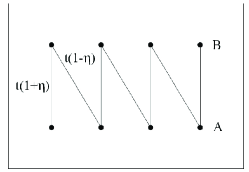
Figure 1: Two-band SSH model of spinless fermions: at each lattice site there are two inequivalent sites, $A$ and $B$, linked by alternating hoppings given by $t(1+\eta)$ and $t(1-\eta)$.

The order parameters for various phases in the interacting system are derived, and are compared to other order parameters, such as the bond-order and charge density wave ones. The topology of the system is affected by the interactions and we use Berry phase to separate the trivial from the topological regions. Interestingly, the derived order parameter appropriate for the topological regions is robust to the presence of inter-site repulsive interactions.

The paper is organized as follows. In Sec. II, we first briefly introduce the scheme to derive the potential order parameters. Then an introduction about the spinless SSH model is given in Sec. III. The topological phase transition in the model is detected by the entanglement entropy and the order parameters for the topologically trivial and non-trivial phases are derived in Sec. IV. In Sec. V, we consider the case when interactions are added. The ground state phase diagram and order parameters for each quantum phases are obtained. The order parameter corresponds to the topological non-trivial phase is further verified by the berry phase results. Finally, a conclusion is given in Sec. VI.

II Outline of the scheme in deriving the potential order operators

To derive the order parameter, we first have to determine the minimum size of the block (sub-system) for which the mutual information (also known as the correlation entropy) does not vanish at a long distance. The mutual information is defined as

$$S(i,j)=S\left({\rho}_{i}\right)+S\left({\rho}_{j}\right)-S\left({\rho}_{i\cup j}\right),$$ (1)

where

$$S\left({\rho}_{i}\right)=-tr({\rho}_{i}\ln{\rho}_{i})$$ (2)

is the von-Neumann entropy of the block $i$. $\rho_{i}$ is the reduced density matrix obtained by tracing out all other degrees of freedom except those of the block $i$, i.e.${\rho}_{i}=$tr$\left|\Psi_{0}\right\rangle\left\langle\Psi_{0}\right|$ where $\left|\Psi_{0}\right\rangle$ is the ground state of the system. If and only if the mutual information is non-vanishing at a long distance, there exists a long-range order (or quasi long range order) in the system MMWolf ; SJGuJPA .

The next step is to calculate the eigenvalues and eigenvectors of the reduced density matrices of the desired block size. Depending on the basis of the reduced density matrix, it is possible to have diagonal and off-diagonal long-range orders. In terms of the creation (annihilation) operator $a_{i\mu}^{\dagger}(a_{i\mu})$ for a state $\left|\mu\right\rangle$ localized at the block $i$, define the diagonal order operator as Gu2013

$$O_{i}^{d}=\sum_{\mu\leq\xi}w_{\mu}a_{i\mu}^{\dagger}a_{i\mu},$$ (3)

where $\xi$ is the rank of $\rho_{i}$. It can be proved that for any $\mu>\xi$, the operator $a_{i\mu}^{\dagger}a_{i\mu}$ does not correlate. The coefficients $w_{\mu}$ can be fixed by the traceless condition tr$(\rho_{i}O_{i}^{d})=0$ and the cut-off condition $\max(\{w_{\mu}\})=1$.

If the two-block reduced density matrix $\rho_{i\cup j}$ is not diagonal in the eigen-basis of $\rho_{i}\otimes\rho_{j}$, there exists off-diagonal long-range order in the system. The corresponding order operator is defined by

$$O_{i}^{o}=\sum_{<\mu,\nu>}w_{\mu\nu}a_{i\mu}^{\dagger}a_{i\nu}+w^{*}_{\mu\nu}a_{i\nu}^{\dagger}a_{i\mu},$$ (4)

where $\mu\neq\nu$ and the sum is over all the pairs of $\mu,\nu$ that correspond to the non-zero off-diagonal matrix elements in $\rho_{i\cup j}$.

III Spinless SSH model

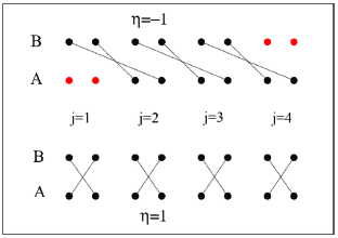
Figure 2: (Color online) Phases of SSH model (or Schockley model). For negative $\eta$ the model is topologically non-trivial with edge states represented by the decoupled Majorana operators (each Majorana is represented by a dot). Since at each end site there are two decoupled Majoranas, these combine to form edge fermionic modes. There is also a trivial phase with no zero energy modes for positive $\eta$.

This model describes a dimerized chain of spinless fermions hopping in a tight-binding band. The dimerization is parametrized by $\eta$. Due to the dimerization the unit cell contains two atoms of types $A$ and $B$. The sites are indexed by $j$. The model is given by the Hamiltonian

$$H=-\mu \sum_{j} \left(n_{j,A}+n_{j,B}\right)$$

$$-t \sum_{j} \left[(1+\eta)c_{j,B}^{\dagger}c_{j,A}+(1+\eta)c_{j,A}^{\dagger}c_{j,B}\right.$$

$$+ \left.(1-\eta)c_{j+1,A}^{\dagger}c_{j,B}+(1-\eta)c_{j,B}^{\dagger}c_{j+1,A}\right].$$

The operator $c_{j,\alpha}$ destroys a spinless fermion at site $j$ of type $\alpha=A,B$, and $n_{j,\alpha}=c_{j,\alpha}^{\dagger}c_{j,\alpha}$. The amplitude $t$ is the hopping, $\eta$ is the dimerization and $\mu$ is the chemical potential. The model is related to the Schockley model yakovenko by taking $t_{1}=t(1+\eta)$ and $t_{2}=t(1-\eta)$. The region of $\eta>0$ corresponds to $t_{1}>t_{2}$ and vice-versa for $\eta<0$. The Hamiltonian in real space mixes nearest-neighbor sites and also has local terms. The links involved are depicted in Fig. 1.

We may define hermitian Majorana operators, $\gamma_{j,\alpha,\beta}$ (with $\beta=1,2$), as

$$c_{j,A} = \frac{1}{2}\left(\gamma_{j,A,1}+i\gamma_{j,A,2}\right),$$

$$c_{j,B} = \frac{1}{2}\left(\gamma_{j,B,1}+i\gamma_{j,B,2}\right).$$ (6)

In terms of Majorana operators the Hamiltonian is written as

$$H = -\frac{\mu}{2}\sum_{j=1}^{N}\left(2+i\gamma_{j,A,1}\gamma_{j,A,2}+i\gamma_{j,B,1}\gamma_{j,B,2}\right)$$

$$- \frac{it}{2}(1+\eta)\sum_{j=1}^{N}\left(\gamma_{j,B,1}\gamma_{j,A,2}+\gamma_{j,A,1}\gamma_{j,B,2}\right)$$

$$- \frac{it}{2}(1-\eta)\sum_{j=1}^{N-1}\left(\gamma_{j+1,A,1}\gamma_{j,B,2}+\gamma_{j,B,1}\gamma_{j+1,A,2}\right)$$

under open boundary condition. Taking $\mu=0$ we have a couple of special points: i) At $\eta=-1$ we have a state with two fermionic-like zero energy edge states, since the four operators $\gamma_{1,A,1},\gamma_{1,A,2};\gamma_{N,B,1},\gamma_{N,B,2}$ are missing from the Hamiltonian. ii) An example of a trivial phase is the point $\eta=1$ in which case there are no zero energy edge states. In Fig. 2 the phases with edge modes are presented for special points in parameter space. The model has simplified time-reversal symmetry and sublattice symmetry, if the chemical potential vanishes. The model is in class BDI and therefore allows the presence of a $Z$ index related to the winding number and the number of edge modes.

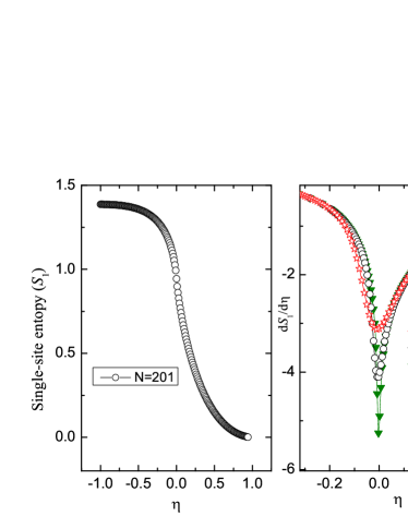
Figure 3: (Color online) Entanglement entropy and its derivative as a function of dimerization.

At the special point of interest $\mu=0,\eta=-1$ shown in the figure, the Hamiltonian reduces to

$$H=it\sum_{j=1}^{N-1}\left(\gamma_{j,B,2}\gamma_{j+1,A,1}-\gamma_{j,B,1}\gamma_{j+1,A,2}\right).$$ (8)

Let us define non-local fermionic operators kitaev

$$d_{j} = \frac{1}{2}\left(\gamma_{j,B,2}+i\gamma_{j+1,A,1}\right),$$

$$d_{j}^{\dagger} = \frac{1}{2}\left(\gamma_{j,B,2}-i\gamma_{j+1,A,1}\right),$$ (9)

and

$$f_{j} = \frac{1}{2}\left(\gamma_{j,B,1}-i\gamma_{j+1,A,2}\right),$$

$$f_{j}^{\dagger} = \frac{1}{2}\left(\gamma_{j,B,1}+i\gamma_{j+1,A,2}\right).$$ (10)

We can show that

$$i\gamma_{j,B,2}\gamma_{j+1,A,1} = 2d_{j}^{\dagger}d_{j}-1,$$

$$-i\gamma_{j,B,1}\gamma_{j+1,A,2} = 2f_{j}^{\dagger}f_{j}-1.$$ (11)

In terms of these new operators we can write that

$$H=t\sum_{j=1}^{N-1}\left(2d_{j}^{\dagger}d_{j}-1+2f_{j}^{\dagger}f_{j}-1\right)$$ (12)

and, therefore, the problem is diagonalized. It is now clear that the ground state is obtained by taking $d_{j}^{\dagger}d_{j}=0$ and $f_{j}^{\dagger}f_{j}=0$ at each site. This new Hamiltonian in terms of the $d$ and $f$ operators is like an Hamiltonian with no hopping and just a chemical potential $\tilde{\mu}=-2t$.

Note that the new operators can be related to the original ones in terms of a non-local transformation as

$$d_{j} = \frac{i}{2}\left(c_{j,B}^{\dagger}-c_{j,B}+c_{j+1,A}+c_{j+1,A}^{\dagger}\right),$$

$$f_{j} = \frac{1}{2}\left(c_{j,B}^{\dagger}+c_{j,B}-c_{j+1,A}+c_{j+1,A}^{\dagger}\right).$$ (13)

Also

$$c_{j,A} = \frac{1}{2}\left[-i(-d_{j-1}^{\dagger}+d_{j-1})-(f_{j-1}-f_{j-1}^{\dagger})\right],$$

$$c_{j,B} = \frac{1}{2}\left[f_{j}^{\dagger}+f_{j}+i(d_{j}+d_{j}^{\dagger})\right].$$ (14)

At the special point we are considering we may also write

$$H=-2t\sum_{j}\left(c_{j+1,A}^{\dagger}c_{j,B}+c_{j,B}^{\dagger}c_{j+1,A}\right).$$ (15)

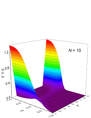
Figure 4: (Color online) Mutual information (correlation entropy) for $N=10$ using OBC. The sub-system is taken as a single-site consisting of two atoms of type A and B.

IV Topological insulator

The evidence that the SSH model has a topologically non-trivial phase can be provided as above, solving the problem in a finite chain using open boundary conditions and showing that there are zero energy edge modes, as shown in Fig. 2. Using the bulk-edge correspondence it can be shown that the winding number is non-trivial in the same phase. Methods inspired by quantum information theory may also be used, such as the entanglement entropy, and is discussed next.

IV.1 Entanglement entropy

The entanglement entropy between a single site and the rest of the chain $S_{1}$ is defined by the von-Neumann entropy in Eq. (2). As shown in Fig. 3, it detects the topological phase transition at $\eta=0$ between the trivial phase and the topological phase. The transition point is particularly visible if one calculates the derivative of the entanglement entropy; It becomes sharper as the system size grows. Even though there is no change of symmetry as one crosses the gapless point, the correlations change and this is detected by the entanglement entropy. In addition, we note that $S_{1}=0$ at $\eta=1$ and $S_{1}=2\ln 2$ at $\eta=0$. This may be explained as follows: When $\eta=1$, the inter-site hopping terms equal to zero. There is no information exchange between different sites. Therefore, $S_{1}$ which measures the entanglement between an arbitrary site and the rest of the chain becomes zero. While for $\eta=0$, the inter-site and intra-site hopping becomes the same. The entanglement for a single site thus reaches its maximum, i.e. $S_{1}=4\times(-\frac{1}{4}\ln\frac{1}{4})=2\ln 2$.

IV.2 Mutual information

In order to implement the method discussed in Sec II, we calculate the mutual information or entropy correlation defined in Eq. (1) in a system with open boundary condition. The sub-system is taken as a single-site consisting of two atoms of type $A$ and $B$. In Fig. 4, $r=|i-j|$ is the distance between sites $i$ and $j$.

For $\eta>0$, the correlation entropy is vanishing exponentially as $r$ grows. For $\eta<0$, there exists correlation between the two ends of the chain indicative of the existence of the edge modes. In a finite system they are coupled and their degeneracy is lifted. In the thermodynamic limit the edge modes become completely decoupled. Around the critical point, $\eta=0$, the correlations extend along the system, signalling the quantum phase transition.

IV.3 Single-site reduced density matrix and order parameters

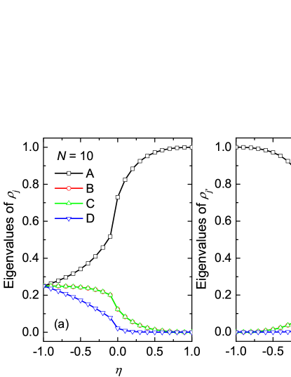
Figure 5: (Color online) Eigenspectrum of the reduced density matrix calculated with a block consisting of (a) an atom A and atom B at site $j$, and (b) an atom B at site $j$ and an atom A at site $j+1$ using PBC for a system of $N=10$.

To derive the order parameter, we calculated the single-site reduced density matrix using periodic boundary condition (PBC). In the basis of $\left|n_{j,A},n_{j,B}\right\rangle=\{\left|00\right\rangle,\left|01\right\rangle,\left|10\right\rangle,\left|11\right\rangle\}$, the reduced density matrix takes the form

$$\rho_{j}=\left(\begin{array}[]{cccc}u&0&0&0\\ 0&v&z&0\\ 0&z&v&0\\ 0&0&0&u\end{array}\right).$$ (20)

The eigenstates are given by

$$|A\rangle = \frac{1}{\sqrt{2}}\left(|10\rangle+|01\rangle\right)$$

$$|B\rangle = |00\rangle$$

$$|C\rangle = |11\rangle$$

$$|D\rangle = \frac{1}{\sqrt{2}}\left(|10\rangle-|01\rangle\right)$$

and the corresponding eigenvalues are shown in Fig. 5(a).

For $\eta<0$, the four eigenstates are equally weighted as $\eta\rightarrow-1$. According to our scheme Gu2013 ; YU2016 , the order parameter can be defined as

$$O_{-} = w_{A}|A\rangle\langle A|+w_{B}|B\rangle\langle B|$$ (22)

$$+w_{C}|C\rangle\langle C|+w_{D}|D\rangle\langle D|.$$

Here we have four variables to be fixed but we only have the traceless and cut-off conditions.

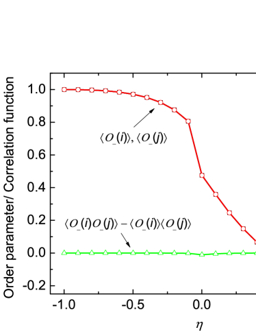
Figure 6: (Color online) Order parameter and the connected correlation function of $O_{-}$ in Eq. (24) as a function of $\eta$.

Instead, we may try a different approach by changing the basis used to define the reduced density matrix. As shown in the previous section, the Hamiltonian is diagonalized in terms of the $d$ and $f$ fermions at the point $\mu=0,\eta=-1$. At this point the reduced density matrix is solely contributed by the $|n_{f}=0,n_{d}=0\rangle$ state. The Hamiltonian is trivially diagonal and the eigenvector of the reduced density matrix is just the eigenvector of the state for which both $d$ and $f$ are empty. (Unlike in the original description in terms of the $c_{A}$ and $c_{B}$ operators, for which all four states contribute equally). So the representation of the states depends on the basis used (meaning which operators we use). Due to the nature of the topological region, one expects that as long as the system remains gapped the properties of the system should be qualitatively the same for all $\eta<0$.

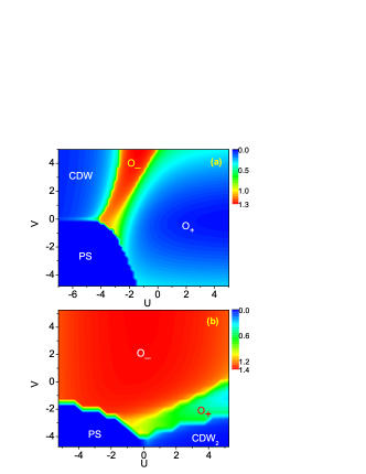
Figure 7: (Color online) Single-site entanglement entropy for (a)$\eta=0.6$ and (b)$\eta=-0.6$ as a function of $U$ and $V$. In each region the dominant order parameters are shown. There is a clear correlation between the entanglement and the order parameter $O_{-}$.

In the diagonal basis the order parameter is

$$O_{-} = |00\rangle\langle 00|$$

$$= I-|10\rangle\langle 10|-|01\rangle\langle 01|-|11\rangle\langle 11|$$

$$= I-f^{\dagger}_{j}f_{j}-d^{\dagger}_{j}d_{j}-f^{\dagger}_{j}f_{j}d^{\dagger}_{j}d_{j}.$$

These expressions are local in space. We may now use the relation between the $d$ and $f$ operators and the original operators in Eq. (13). This is a non-local transformation since it couples site $j$ with the nearest-neighbor site $j+1$. The operator may now be obtained as

$$O_{-} = \frac{3}{2}\left(c_{j+1,A}^{\dagger}c_{j,B}+c_{j,B}^{\dagger}c_{j+1,A}\right)$$ (24)

$$+ n_{j,B}n_{j+1,A}-\frac{1}{2}\left(n_{j,B}+n_{j+1,A}\right).$$

For $\eta>0$, the mutual information is exponentially vanishing and the correlation is not captured by considering the single-site block with atoms A and B. However, one could take the block consisting of an atom B at site $j$ and an atom A at site $j+1$. The mutual information obtained would be the mirror image of that in Fig. 4 about $\eta=0$. The eigenspectrum in this case is shown in Fig. 5(b). Carrying out similar analysis as above, the order parameter takes the form of Eq. (24), but with the index $\{j+1,A\}$ and $\{j,B\}$ being replaced by $\{j,B\}$ and $\{j,A\}$, respectively. We have

$$O_{+} = \frac{3}{2}\left(c_{j,B}^{\dagger}c_{j,A}+c_{j,A}^{\dagger}c_{j,B}\right)$$ (25)

$$+ n_{j,A}n_{j,B}-\frac{1}{2}\left(n_{j,A}+n_{j,B}\right).$$

In Fig. 6, we show the results for the order parameter $O_{-}$ and its correlation function as a function of the dimerization $\eta$ (for $O_{+}$ could be obtained by taking the mirror image about $\eta=0$). By construction we see that the order parameter is dominant in its intended region of applicability and change continuously from a finite value towards zero or small values as we move to the opposite region. However, since the system is actually not ordered the connected correlation function $\langle O_{i}O_{j}\rangle-\langle O_{i}\rangle\langle O_{j}\rangle$ vanishes in all regimes.

IV.4 Discussion

Regarding the above derivations, note that the dominating eigenstate of the reduced density matrix is given by a single state in the basis chosen. This is in contrast with the case of a continuous phase transition in which symmetric eigenstates would be resulted in a finite system. Consequently, we did not apply the traceless condition and the cut-off conditions in the derivation. The resulted order parameters, despite showing a sharp change around the quantum critical point, do not behave as conventional ones (finite in the ”ordered” phase and goes to zero in the ”disordered” phase). The order parameters are defined accross two lattice locations: at the same site between the two types of (sublattice) locations $A$ and $B$ for $\eta>0$, and linking two locations $A$ and $B$ between neighboring sites. A vanishing order parameter may be constructed summing two consecutive links with opposite signs as in the bond-order (BOW) parameter benthien .

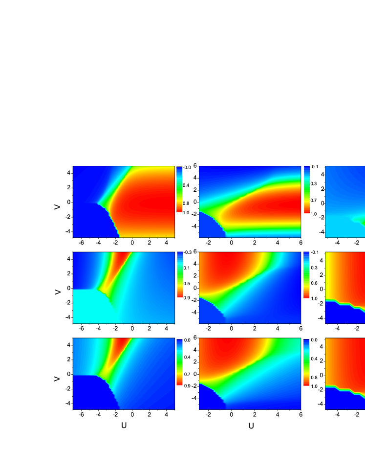
Figure 8: (Color online) Order parameters suitable for $\eta=0.6,\eta=0,\eta=-0.6$ (from left to right). In the first row for $O_{+}$ given in Eq. (25). In the second row $O_{-}$ given in Eq. (24). In the third row for $m_{\textrm{BOW}}$ given in Eq. (27).

The order parameter in the topological region is similar to the BOW order parameter, with a few more terms related to the densities at sites $A$ and $B$.

V Effect of interactions

Adding interactions is interesting because i) allows a generalization of the procedure of finding order parameters to a problem that is now interacting and to determine how the interactions affect the choice of order parameter(s) to describe the various phases, and ii) may change the topological properties determined for the non-interacting system.

V.1 DMRG results for order parameters

We add a local Hubbard-$U$ like term (coupling two electrons at the same site but in two different sublattices, $A$ and $B$) and/or a $V$-term coupling two electrons at nearest-neighbor sites.

In the presence of interactions the model Hamiltonian is chosen as

$$H = -\sum_{j}\left[\left(1+\eta\right)c_{j,A}^{\dagger}c_{j,B}+\left(1-\eta\right)c_{j,B}^{\dagger}c_{j+1,A}+h.c.\right]$$ (26)

$$+ U\sum_{j}n_{j,A}n_{j,B}+V\sum_{j}n_{j,B}n_{j+1,A}$$

We calculate, using the infinite density matrix renormalization group method white with PBC, the entanglement entropy and various order parameters as a function of $\eta,U$ and $V$. The truncation error is set to less than $10^{-7}$ in our calculations. The system size simulated is $N=86$ unless otherwise specified. Specifically we calculate in addition to the order parameters $O_{+}$ and $O_{-}$, a bond-order parameter defined on a link

$$m_{\textrm{BOW}}=\langle\left(c_{j+1,A}^{\dagger}c_{j,B}+H.c.\right)\rangle.$$ (27)

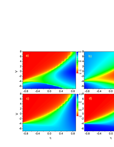
Figure 9: (Color online) (a) Single-site entanglement entropy, and order parameter (b) $O_{+}$, (c) $O_{-}$, (d) $m_{\textrm{BOW}}$ for $U=0$ as a function of $V$ and $\eta$.

We begin by accessing the effect of the interaction on the single-site entanglement entropy shown in Fig. 7 for a point in the trivial region with $\eta=0.6$ and another point in the topological region with $\eta=-0.6$ as a function of the interactions $U$ and $V$. The smoothness of the phase boundaries were limited by the point density of the driving parameters. As shown in Fig. 3, the entanglement entropy is large in the topological region with no interactions. The presence of repulsive inter-site interaction $V$ does not change the entanglement entropy. However, if $V<0$, the entanglement entropy is reduced, particularly when $U<0$. The decrease of the entanglement entropy is more gradual if $U>0$. In the trivial region ($\eta>0$), the entanglement is also large in the regime where the order parameter $O_{-}$ has a large value.

In Fig. 8 we compare various order parameters for three points: one in the topological trivial region ($\eta=0.6$), one at the transition point where the dimerization $\eta=0$, and one in the topological region ($\eta=-0.6$). The results are presented as a function of the interactions $U$ and $V$.

A first comment is that there is some interpolation between the topological and the trivial regions as one crosses the transition point. At least from the point of view of the order parameters, there does not seem to be a clear distinction between the two topologically different regimes. This is consistent with the idea that a topological transition is subtle and is not straightforwardly associated with a change of some order parameters. However, it is the purpose of the choice of order parameters by analysing the reduced density matrix eigenstates and eigenvlaues to construct order parameters without the necessary use of any symmetry breaking arguments. The similarity of the order parameters $m_{\textrm{BOW}}$ and $O_{-}$ might lead to the expectation that, at least in this case, the method is actually capturing the traditional types of order (as also revealed in the mutual information results) instead of some form of topological property.

The order parameters $m_{\textrm{BOW}}$ and $O_{-}$ are particularly expanded in the phase diagram in the topological regime. Their extension decrease as one crosses over to the trivial region, as might be expected since they are particularly suited to the topological region.

As one crosses to the trivial region, the effect of $U$ (local term) becomes more prominent as evidenced by the local nature of the order parameter $O_{+}$. As expected the effect of the interactions is smaller in the trivial regime where extended regions in the phase diagram result in a large value of this order parameter.

Given that the effect of the local interaction, $U$, is small particularly in the topological regime, we take $U=0$ in Fig. 9 and study the effect on the order parameters and the single-site entanglement entropy as a function of $V$ and $\eta$. We clearly see the dominance of the order parameters $O_{-}$ and $m_{\textrm{BOW}}$ in the topological region of $\eta<0$ and of the order parameter $O_{+}$ in the trivial regime $\eta>0$.

The order parameters considered so far are only defined in single links. In order to probe possible long-range order we need to consider two cells containing at least two consecutive links. One may consider possible related order parameters defined as follows:

$$O_{\textrm{BOW}}=\left\langle\left(c^{\dagger}_{j+1,B}c_{j,A}+H.c.\right)-\left(c^{\dagger}_{j,B}c_{j,A}+H.c.\right)\right\rangle$$ (28)

for bond-ordering (BOW) and

$$O_{\textrm{CDW}}=\frac{1}{2}\left\langle\left(n_{j+1,A}+n_{j+1,B}-1\right)-\left(n_{j,A}+n_{j,B}-1\right)\right\rangle$$ (29)

for charge-density wave (CDW) ordering.

The analysis of several partial links is shown in Fig. 10, which leads to the conclusion that the electron configurations may be described by the scenario show in Fig. 11.

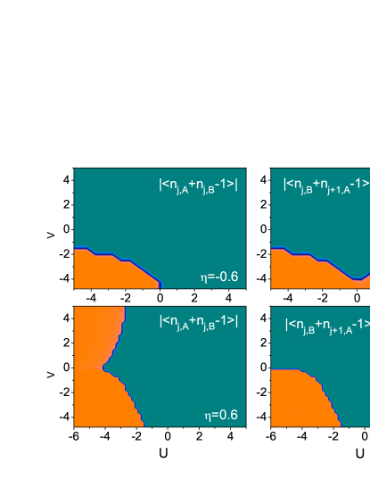
Figure 10: (Color online) Electron number density analysis on different links: (left column) A and B at the same site, (right column) A and B linked by different sites. The fist row is for $\eta=-0.6$ and the second row is for $\eta=0.6$.

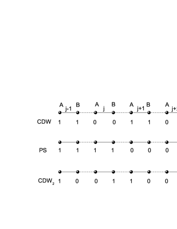
Figure 11: Possible electron configuration for the three quantum states indicated in Fig. 10.

The order parameters related to BOW and CDW as a function of $U$ and $V$ are presented in Fig. 12 and Fig. 13 respectively. The results for the BOW order parameter are consistent with those obtained from the derived order parameters $O_{+}$ and $O_{-}$ in the previous section. In the case without interactions ($U=0,V=0$), $O_{+}$ dominates, and $O_{\textrm{BOW}}<0$ and is close to $-1$ in the trivial region. While in the topological region, the order parameter $O_{-}$ dominates, and $O_{\textrm{BOW}}>0$ and is close to $1$. The effect of interactions is similar to the one observed for the link order parameters. On the other hand, the result in 13(a) shows that the inter-site repulsion ($V>0$) and the intra-site attraction ($U<0$) between the electrons favor the CDW order in Fig. 11. According to the analysis on electron configurations, we could define another order parameter

$$O_{\textrm{CDW${}_{2}$}} = \frac{1}{2}\left\langle\left(n_{j+1,B}+n_{j+2,A}-1\right)\right.$$ (30)

$$\hskip 18.0pt\left.-\left(n_{j,B}+n_{j+1,A}-1\right)\right\rangle,$$

which describes the charge-density wave of the links between adjacent sites. The nonzero values appear at the $\eta=-0.6$ case as shown in Fig. 13(b). We therefore conclude the nonzero region, which corresponds to the $\mathrm{CDW}_{2}$ region in Fig. 7, belongs to the $\mathrm{CDW}_{2}$ order.

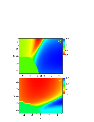
Figure 12: (Color online) BOW order parameter of eq. (28) for (a) $\eta=0.6$ and (b) $\eta=-0.6$.

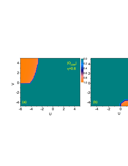
Figure 13: (Color online)(a) CDW order parameter of eq. (29) for $\eta=0.6$. Because $O_{CDW}=0$ at the whole parameter region for $\eta=-0.6$, we do not show it here. (b) $\mathrm{CDW}_{2}$ order parameter of eq. (30) for $\eta=-0.6$.

V.2 Berry phase in the presence of interactions

To see if and how the topology changes one needs to look at edge states (using open boundary conditions) or looking at topological invariants (using periodic boundary conditions). One method to calculate a topological invariant involves calculating the Green’s function and using the definitions of the invariants manmana . Another possibility to study a topological invariant is to calculate the Berry phase berry1 ; berry2 .

Using twisted boundary conditions we can calculate the Berry phase which is a topological invariant that reveals the topological nature of the system. Imposing a phase of $\phi$ in the boundary conditions the Berry phase may be calculated as

$$\gamma=-i\int_{0}^{2\pi}\langle\psi(\phi)|\frac{\partial}{\partial\phi}\psi(\phi)\rangle.$$ (31)

In order to calculate the Berry phase, it is more convenient to discretize the range of phase values into $M$ points, i.e. $\phi_{1},\phi_{2},\cdots,\phi_{M}$. Defining the link variable $U(\phi_{l})=\psi^{*}(\phi_{l})\psi(\phi_{l+1})$ and summing over $\phi_{l}$, we may obtain the Berry phase as

$$\gamma=-i\sum_{l=1}^{M}\ln U(\phi_{l}).$$ (32)

Consider first the non-interacting case. In Fig. 14 the results for the Berry phase as a function of $\eta$ in the absence of interactions is shown. In the topological region the Berry phase is $\pi$ and in the trivial phase it vanishes, as expected of the topological transition discussed above. We performed ED for small systems to calculate the overlap between the groundstate at nearby values of the phase imposed by twisted boundary conditions.

Figure 14: Berry phase as a function of $\eta$ for the non-interacting case.

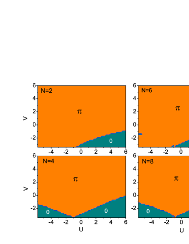
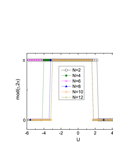
Figure 15: (Color online) Berry phase as a function of the interactions for $\eta=-0.6$ for various system sizes.

In Fig. 15 we analyze the size dependence of the Berry phase for $\eta=-0.6$. As is well known, the $V$ term may induce bond-order which is a characteristic feature of the topological region. Starting from the topological region we see that both negative $V$ and negative $U$ affect the topology and a trivial regime characterized by the vanishing Berry phase may appear as a result. In Fig. 15 we also consider the size dependence of the results for $\eta=-0.6$. Due to finite size effects there is a $4N$, $4N+2$ alternancy. In the very large size limit the results converge to the $4N$-case, as shown in the right plot of Fig. 15, where the curves of Berry phase for $V=-2.0$ tends to the same value as $N$ is larger than 10 (system sizes up to $N=12$ is considered here).

To illustrate the relationship between the topological phase and the derived order parameter $O_{-}$, Fig. 16 plots the Berry phase and $O_{-}$ under the same parameter’s conditions. The points where $O_{-}$ changes dramatically is consistent with the edge of the topological $\pi$ region of the Berry phase. Therefore, the dominant region of $O_{-}$ indeed describes the topologically non-trivial phase. In addition, the Berry phase for $\eta=0.6$ is also $\pi$ when $O_{-}$ is dominant due to the effect of interactions (negative U positive V, as shown in Fig. 12). This confirms the appearance of topology due to the interactions having started at $U=0$ and $V=0$ from a trivial phase. Also, it extends the relationship between a Berry phase of $\pi$ and a non-zero $O_{-}$.

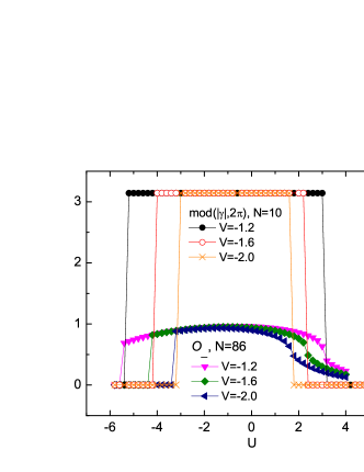
Figure 16: (Color online) Berry phase and order parameter $O_{-}$ as a function of $U$ under different $V$. The dominant region of $O_{-}$ coincides with the topological phase indicated by the $\pi$ value of Berry phase.

V.3 Reduced density matrix and order parameters in the presence of interactions

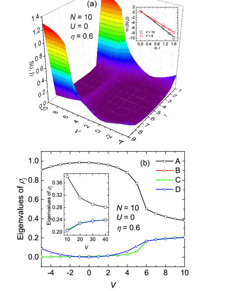
Figure 17: (Color online) (a) Mutual information as a function of $V$ and distance $r=|i-j|$ for $U=0,\eta=0.6$. Inset shows that the mutual information decays algebraically with the distance. (b) The eigenspectrum of the reduced density matrix $\rho_{j}$ as a function of $V$. Inset shows the asymptotic weight of the eigenstates of the reduced density matrix in the large $V$ limit.

V.3.1 $\eta=0.6$

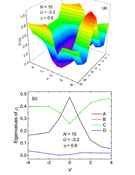
Figure 18: (Color online)(a) Mutual information as a function of $V$ and distance $r$ for $U=-3.2,\eta=0.6$. (b) The eigenspectrum of the reduced density matrix $\rho_{j}$ as a function of $V$.

Let us first consider varying $V$ along the path of fixed $U=0$. The mutual information as a function of $V$ and the distance $r$ calculated for $U=0$ with PBC is shown in Fig. 17(a). As indicated by the log-log plot in the inset, the mutual information decays algebraically with the distance and we could argue that there exist a long-range correlation in the system for $V>6$.

Figure 17(b) shows the eigenvalues of the states in Eq. (LABEL:eq:Estates) of the single-site reduced density matrix. For $V>6$, the contribution of the four eigenstates are similar and they are almost equally weighted in the large $V$ limit (inset of 17(b)). This is the same as the case for $\eta<0$ in the non-interacting system. Following the same argument in Sec. IV.3, the order parameter for this phase is $O_{-}$ in Eq. (24).

For $V<6$, from the result of single-site entanglement show in Fig. 7, the system is in the same phase as that of $U=V=0$. The behavior of the reduced density matrix eigenspectrum is the same as for the non-interacting case for $\eta>0$. The order parameter in this regime is $O_{+}$ as obtained in Eq. (25).

To analyze the different possible phase regions in Fig. 7, we next consider the path along fixed $U=-3.2$. Figure 18 shows the mutual information as a function of $r$ and $V$. Obviously, the mutual information for $V>2$ and $V<-2$ (corresponding to CDW and PS phases in Fig. 7 respectively) is non-vanishing at a long distance. In Fig. 18(b), the eigenspectrum of the reduced density matrix is dominated by the states $\left|B\right\rangle$ and $\left|C\right\rangle$ for both regions. For large enough system, the weight of state $\left|A\right\rangle$ would be suppressed to zero (our DMRG results, which we do not show here, indicate this). We can define the order parameter as

$$O_{3}=w_{B}\left|B\right\rangle\left\langle B\right|+w_{C}\left|C\right\rangle\left\langle C\right|.$$ (33)

Using the traceless condition, we have $w_{B}=-w_{C}$ and applying the cut-off condition, i.e. $w_{B}=1$, we have

$$O_{3} = \left|00\right\rangle\left\langle 00\right|-\left|11\right\rangle\left\langle 11\right|,$$ (34)

$$= 1-(n_{j,A}+n_{j,B}),$$

which is indeed the order parameter for the CDW and PS phases. To further distinguish the two phases, we can consider the correlation function in the momentum space shown in Fig. 19. The correlation function peaks at $2\pi/N$ (and $2\pi(N-1)/N$ as a result of PBC) and $\pi$ for $V<-2$ and $V>2$, respectively. It indicates that the electronic configuration has a wavelength of half of the lattice in the former case and of two sites in the latter case. This is consistent with our deduction for the PS and CDW phases illustrated in Fig. 11. In addition, the behavior of the mutual information in Fig. 18(a) also reflects the difference of the two phases. In the PS phase, the largest correlation appears between two local sites separated by half of the lattice.

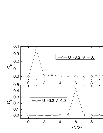
Figure 19: The correlation function of $O_{3}$ in the momentum space for $U=-3.2$ and $V=\pm 4$. Here $k=2m\pi/N$, where $m=0,1,\cdots,N-1$.

V.3.2 $\eta=-0.6$

Consider now the case $U=4$. Figure 20 shows the mutual information as a function of $V$ and $r$. In the case of $V>0$, a correlation emerges between the end points of the system. Note from Fig. 8 that in this regime $O_{-}$ also becomes large. On the other hand, for $V<0$, the Berry phase results of Fig. 15 do not indicate a topological phase, consistent with the separation of the two types of properties. For negative $V<-2.5$ the correlation extends all over the system, as expected.

Figure 21(a) shows the eigenvalues of the states $\{A,B,C,D\}$ of the reduced density matrix. For $V>0$, all the eigenstates have non-negligible weight. Let us once again transform into the basis defined by the $d$ and $f$ operators using Eq. (14). Under PBC and keeping the number of electrons equal to the number of sites (half-filling) the transformed Hamiltonian reads $H=H_{1}+H_{2}$ where

$$H_{1} = \frac{t}{2}\left(1+\eta\right)\sum_{j=1}^{N}\left(f_{j}^{\dagger}f_{j+1}^{\dagger}+f_{j+1}f_{j}+f_{j}^{\dagger}f_{j+1}+f_{j+1}^{\dagger}f_{j}\right)$$ (35)

$$+ \frac{t}{2}\left(1+\eta\right)\sum_{j=1}^{N}\left(d_{j}^{\dagger}d_{j+1}^{\dagger}+d_{j+1}d_{j}+d_{j}^{\dagger}d_{j+1}+d_{j+1}^{\dagger}d_{j}\right)$$

$$+ \left[t(1-\eta)+\frac{V}{2}\right]\sum_{j=1}^{N}\left(n_{j}^{f}+n_{j}^{d}\right)$$

$$- V\sum_{j=1}^{N}n_{j}^{f}n_{j}^{d}+N\left[\frac{U}{4}-t(1-\eta)\right],$$

and

$$H_{2} = -\frac{U}{4}\sum_{j=1}^{N}\left(f_{j}^{\dagger}f_{j+1}d_{j}^{\dagger}d_{j+1}+f_{j+1}^{\dagger}f_{j}d_{j+1}^{\dagger}d_{j}\right.$$ (36)

$$+ \left.f_{j+1}^{\dagger}f_{j}d_{j}^{\dagger}d_{j+1}+f_{j}^{\dagger}f_{j+1}d_{j+1}^{\dagger}d_{j}\right.$$

$$+ \left.f_{j}f_{j+1}d_{j+1}^{\dagger}d_{j}^{\dagger}+f_{j+1}^{\dagger}f_{j}^{\dagger}d_{j}d_{j+1}\right.$$

$$+ \left.f_{j}^{\dagger}f_{j+1}^{\dagger}d_{j}^{\dagger}d_{j+1}^{\dagger}+f_{j+1}f_{j}d_{j+1}d_{j}\right.$$

$$- \left.f_{j+1}^{\dagger}f_{j}^{\dagger}d_{j}^{\dagger}d_{j+1}-f_{j}f_{j+1}d_{j+1}^{\dagger}d_{j}\right.$$

$$- \left.f_{j}^{\dagger}f_{j+1}d_{j+1}^{\dagger}d_{j}^{\dagger}-f_{j+1}^{\dagger}f_{j}d_{j}d_{j+1}\right.$$

$$- \left.f_{j+1}^{\dagger}f_{j}d_{j+1}^{\dagger}d_{j}^{\dagger}-f_{j}^{\dagger}f_{j+1}d_{j}d_{j+1}\right.$$

$$- \left.f_{j}f_{j+1}d_{j}^{\dagger}d_{j+1}-f_{j+1}^{\dagger}f_{j}^{\dagger}d_{j+1}^{\dagger}d_{j}\right).$$

In the basis of $|n_{j}^{f},n_{j}^{d}\rangle$ the eigenstates of the single-site reduced density matrix take the form

$$|A^{\prime}\rangle = \alpha|10\rangle+\beta|01\rangle,$$

$$|B^{\prime}\rangle = |00\rangle,$$

$$|C^{\prime}\rangle = |11\rangle,$$

$$|D^{\prime}\rangle = \beta|10\rangle-\alpha|01\rangle.$$ (37)

As shown in Fig. 21(b), the state $\left|B^{\prime}\right\rangle$ is dominant in the region $V>0$ and we would arrive at the same order parameter, i.e. $O_{-}$, as in the case of no interaction. The order parameter in this topological region prevails and is not affected by the interactions.

For $V<-2.5$, states $\left|A\right\rangle$ and $\left|D\right\rangle$ dominant and let us define the order parameter as

$$O_{+,1} = w_{A}|A\rangle\langle A|+w_{D}|D\rangle\langle D|$$ (38)

$$= \frac{1}{2}\left(w_{A}+w_{D}\right)\left(|10\rangle\langle 10|+|01\rangle\langle 01|\right)$$

$$+ \frac{1}{2}\left(w_{A}-w_{D}\right)\left(|10\rangle\langle 01|+|01\rangle\langle 10|\right).$$

Without the loss of generality, assume that the weights of the two states $\left|A\right\rangle$ and $\left|D\right\rangle$ tends to an asymptotic value of 0.5 with some probably chosen values of $U$ and $V$ within the same phase. Traceless condition then gives $w_{A}=-w_{D}$ and setting $w_{A}=1$, we have

$$O_{+,1}=c_{j,A}^{\dagger}c_{j,B}+c_{j,B}^{\dagger}c_{j,A}.$$ (39)

A remark here is that if one consider the form of Hamiltonian in Eq. (26), the case of a positive $\eta$ is equivalent to the case of a negative $\eta$ with the role of $U$ and $V$ interchanged and $\{j,A\},\{j,B\}$ being replaced by $\{j,B\},\{j+1,A\}$ respectively. Therefore, for the case $V<-2.5$, one can also take $O_{3}$ in Eq. (34) but with the index replaced as the order parameter. That gives

$$O_{+,2}=1-(n_{j,B}+n_{j+1,A}),$$ (40)

which is consistent with the $\mathrm{CDW}_{2}$ order parameter. In addition, the linear combination of $O_{+,1}$ and $O_{+,2}$ can also be an order parameter.

For $-2.5<V<0.5$, note that the eigenspectrum is similar to the one show in the $V<6$ regime in Fig. 17(b) and supplemented with the above argument, the order parameter for this phase is given by $O_{+}$.

Figure 20: (Color online) (a) Mutual information as a function of $V$ and distance $r$ for $U=4,\eta=-0.6$ calculated with PBC. (b) Mutual information as a function of $r$ for $V=6,8$ calculated with OBC.

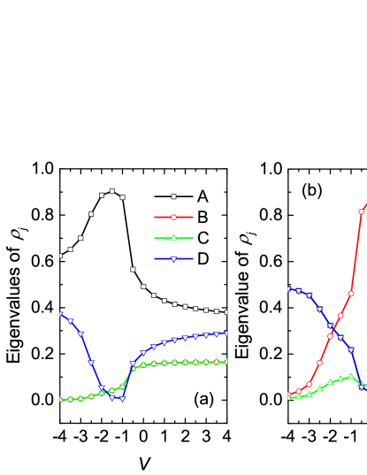
Figure 21: (Color online) Eigenspectrum of the single-site reduced density matrix in the (a) original basis, and (b) rotated basis as a function of $V$. Here $N=10$, $U=4$ and $\eta=-0.6$.

VI Conclusions

Using the method proposed from the reduced density matrixGu2013 , we construct the potential order parameters for a condensed matter system, especially for the topologically non-trivial phase, which can not be described by those general order parameters derived from the landau’s symmetry breaking theory. We first study the two-band spinless fermions SSH model. In this simple model, a topological phase transition exists. We calculate the entanglement entropy, which clearly identify the quantum critical point. Analyzing the mutual information and one-site reduced density matrix, we get a local order parameter for the trivial phase. Furthermore, through an appropriate change of basis by representing the Hamiltonian in a Majorana fermion basis, we reduced the number of eigenvalues that contribute significantly and construct the non-local order parameter $O_{-}$ for the topologically non-trivial phase.

We then consider the case when the interactions $U$ and $V$ are added. The entanglement entropy results capture a rich ground state phase diagram on the $U-V$ plane. Through analysing the electron configurations, we identify the $\mathrm{PS}$, $\mathrm{CDW}$, and $\mathrm{CDW}_{2}$ phases, and give the order parameter for the $\mathrm{CDW}_{2}$ state. The order parameters for various quantum phases are deduced according to the method of analyzing the mutual information and the reduced density matrix spectra. In addition, comparing with the dominant regions of different order parameters, we conclude that the topologically trivial and non-trivial quantum phases described by $O_{+}$ and $O_{-}$, respectively, could exist in a wide range of parameter space. Moreover, the topology of the system affected by the interactions is verified by the Berry phase results, and the effectiveness of the deduced order parameter $O_{-}$ in describing the topological quantum phase is further proved.

- (1) S. Sachdev, Quantum Phase Transitions, (Cambridge University Press, Cambridge, UK, 2000).
- (2) L. Carr, Understanding Quantum Phase Transitions, (CRC Press, 2011).
- (3) X. G. Wen, Qunatum Field Theory of Many-body Systems, (Oxford University, New York, 2004).
- (4) L. Amico, R. Fazio, A. Osterloh, and V. Vedral, Rev. Mod. Phys. 80, 517 (2008).
- (5) T. J. Osborne and M. A. Nielsen, Phys. Rev. A 66, 032110 (2002).
- (6) A. Osterloh, L. Amico, G. Falci, and R. Fazio, Nature 416, 608 (2002).
- (7) S.J. Gu, H.Q. Lin, Y.Q. Li, Phys. Rev. A 68 042330 (2003); S.J. Gu, G.S. Tian, H.Q. Lin, Phys. Rev. A 71 052322 (2005); S.J. Gu, S.S. Deng, Y.Q. Li, H.Q. Lin, Phys. Rev. Lett. 93 086402 (2004).
- (8) M. Levin, X.G. Wen, Phys. Rev. Lett. 96 110405 (2006).
- (9) A. Kitaev, J. Preskill, Phys. Rev. Lett. 96 110404 (2006).
- (10) S. J. Gu, W. C. Yu, and H. Q. Lin, Ann. Phys. 336, 118 (2013).
- (11) W.C. Yu, S.J. Gu and H.Q. Lin, Eur. Phys. J. B 89 212 (2016).
- (12) S. Furukawa, G. Misguich, and M. Oshikawa, Phys. Rev. Letts. 96, 047211 (2006).
- (13) C. L. Henley and H. J. Changlani, J. Stat. Mech. P11002 (2014).
- (14) S.-A. Cheong and C. L. Henley, Phys. Rev. B 79, 212402 (2009).
- (15) W.P. Su, J.R. Schrieffer, A.J. Heeger, Phys. Rev. Lett. 42, 1698 (1979): Phys. Rev. B 22, 2099 (1980); A.J. Heeger, S- Kivelson, J.R. Schrieffer and W.P. Su, Rev. Mod. Phys. 60; 781 (1988).
- (16) M. Z. Hasan and C. L. Kane, Rev. Mod. Phys. 82, 3045 (2010)
- (17) X.-L. Qi and S.-C Zhang, Rev. Mod. Phys. 83, 1057 (2011).
- (18) A.P. Schnyder, S. Ryu, A. Furusaki and A.W.W. Ludwig, Phys. Rev. B 78, 195125 (2008).
- (19) S.S. Pershoguba and V.M. Yakovenko, Phys. Rev. B 86, 075304 (2012).
- (20) S.R. White et al., Density-Matrix Renormalization: A new numerical method in physics (Berlin:Springer, 1999).
- (21) C.L. Wang, W.Z. Wang, C.L. Gu, Z.B. Su and L. Yu, Phys. Rev. B 48, 10788 (1993).
- (22) E. Jeckelmann, Phys. Rev. B 57, 11838 (1998).
- (23) J. Riera and D. Poilblanc, Phys. Rev. B 62, R16243 (2000).
- (24) Y.Z. Zhang, C.Q. Wu and H.Q. Lin, Phys. Rev. B 72, 125126 (2005).
- (25) H. Benthien, F.H.L. Essler and A. Grage, Phys. Rev. B 73, 085105 (2006).
- (26) D.K. Campbell, J. Tinka Gammel and E.Y. Loh, Jr., Phys. Rev. B 42, 475 (1990).
- (27) S. Ejima, F. Gebhard and S. Nishimoto, Phys. Rev. B 74, 245110 (2006).
- (28) M. Kumar, S. Ramasesha and Z.G. Soos, Phys. Rev. B 79, 035102 (2009).
- (29) M. Weber, F.F. Assaad and M. Hohenadler, Phys. Rev. B 91, 245147 (2015).
- (30) M. Nakamura, J. Phys. Soc. Jpn. 68, 3123 (1999); Phys. Rev. B 61, 16377 (2000).
- (31) P. Sengupta, A.W. Sandvik and D.K. Campbell, Phys. Rev. B 65, 155113 (2002).
- (32) Y.Z. Zhang, Phys. Rev. Lett. 92, 246404 (2004)
- (33) S. Ejima and S. Nishimoto, Phys. Rev. Lett. 99, 216403 (2007).
- (34) M. M. Wolf, F. Verstraete, M. B. Hastings, and J. I. Cirac, Phys. Rev. Lett. 100, 070502 (2008).
- (35) S. J. Gu, C. P. Sun, and H. Q. Lin, J. Phys. A: Math. Theor. 41, 025002 (2008).
- (36) A. Y. Kitaev, Phys.-Usp. 44, 131 (2001).
- (37) S.R. Manmana, A.M. Essin, R.M. Noack and V. Gurarie, Phys. Rev. B 86, 205119 (2012).
- (38) H. Guo and S.Q. Shen, Phys. Rev. B 84, 195107 (2011).
- (39) H. Guo, S.Q. Shen and S. Feng, Phys. Rev. B 86, 085124 (2012).