Classification of Crescent Configurations

Abstract.

Let $n$ points be in crescent configuration in $\mathbb{R}^{d}$ if they lie in general position in $\mathbb{R}^{d}$ and determine $n-1$ distinct distances, such that for every $1\leq i\leq n-1$ there is a distance that occurs exactly $i$ times. Since Erdős’ conjecture in 1989 on the existence of $N$ sufficiently large such that no crescent configurations exist on $N$ or more points, he, Pomerance, and Palásti have given constructions for $n$ up to $8$, but nothing is yet known for $n\geq 9$. Most recently, Burt et. al. [BGMMPS] had proven that a crescent configuration on $n$ points exists in $\mathbb{R}^{n-2}$ for $n\geq 3$. In this paper, we study the classification of configurations on $4$ and $5$ points using distance classes. Our techniques, together with A. Liu’s 1986 result [Liu], give all distance classes with realizable configurations on $4$ points, and a lower bound on the number of configurations on $5$ points. Furthermore, since they can be generalized to higher dimensions, our techniques offer a new viewpoint on the problem through the lens of distance geometry, and provide a systematic way to construct crescent configurations.

1. Introduction

Erdős once wrote, “my most striking contribution to geometry is, no doubt, my problem on the number of distinct distances,” [Erd96]. The referred question, which asks what is the minimum number of distinct distances determined by $n$ points, was first asked in 1946 [Erd46] and marked the beginning of a chain of variants. See [She] and [BGMMPS] for a survey on these. Although one would expect all distances between $n$ points to be different if they were to be placed in the plane at random, if the distances are regularly placed, such as on a lattice, then many distances may repeat. Erdős’ conjectured lower bound, $\Omega(n/\sqrt{\log{n}})$, attained by a $\sqrt{n}\times\sqrt{n}$ integer lattice, was essentially proven up to a $\sqrt{\log{n}}$ factor by Guth and Katz in 2010. [GK]

The variant we study in this paper is one where the distances have prescribed multiplicities. One says $n$ points are in crescent configuration in $\mathbb{R}^{d}$ if they are in general position and determine $n-1$ distinct distances such that for every $1\leq i\leq n-1$, there is a distance that occurs exactly $i$ times. Erdős conjectured that there exists a sufficiently large $N$ such that no crescent configuration exists on $N$ or more points [Erd89]. Though constructions have been provided for $n=5,6,7,8$ by Erdős, I. Palásti and C. Pomerance [Pal87, Pal89, Erd89], little progress has been made towards a construction for $n\geq 9$. One problem often encountered in the search for these configurations is the lack of understanding of their properties, and the difficulty in exhibiting the configurations’ information combinatorially.

Later, A. Liu published a manuscript in which he lists known crescent configurations, and begins classifying crescent configurations (which he refers to as complete systems on $n$ points) based on their labeled graph structures [Liu]. In particular, he identified 3 combinatorial types of crescent configurations on 4 points.

As such, we continue this approach to studying these crescent configurations, working to formalize Liu’s idea of classifying these configurations using combinatorial data. Along the way, we borrow techniques from distance geometry and graph theory. In our methods, we employ a concept of strict distance classes, which are distance classes of crescent configurations which are more likely to obey general position. Our main theorems are the results of two algorithms that search for and classify crescent configurations on any $n\geq 4$ up to strict distance class, and find geometric realizations for one member of each of these distance classes in the plane.

Theorem 1.1.

Given a set of three distinct distances $\{d_{1},d_{2},d_{3}\}$ on four points, there are only three strict distance classes with allowable crescent configurations. In Figure 2 we provide graph realizations for each type.

Remark 1.2.

Types M and C were found by Liu, but type R does not appear in his manuscript. Instead, Liu presents a third type in which the four points form the corners of a parallelogram. We do not include this here, because this parallelogram type is not a strict distance class; it is in the same distance class as configurations that violate general position. Refer to Remark 3.6 for more details on this exclusion. However, together with Liu’s result, we obtain a complete classification of distance classes on four point with allowable crescent configurations.

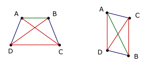
Figure 1. Liu’s parallelogram, shown on the right, has the same distance set as the trapezoid on the left. This trapezoid violates general position, thus the parallelogram does not have a strict distance class.

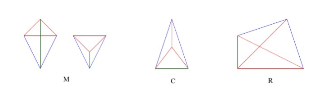
Figure 2. Types M, C, and R.

Theorem 1.3.

Given a set of four distinct distances $\{d_{1},d_{2},d_{3},d_{4}\}$ on five points, there are at least 27 strict distance classes with allowable crescent configurations. In Figure 3 we provide the graph realizations for each type.

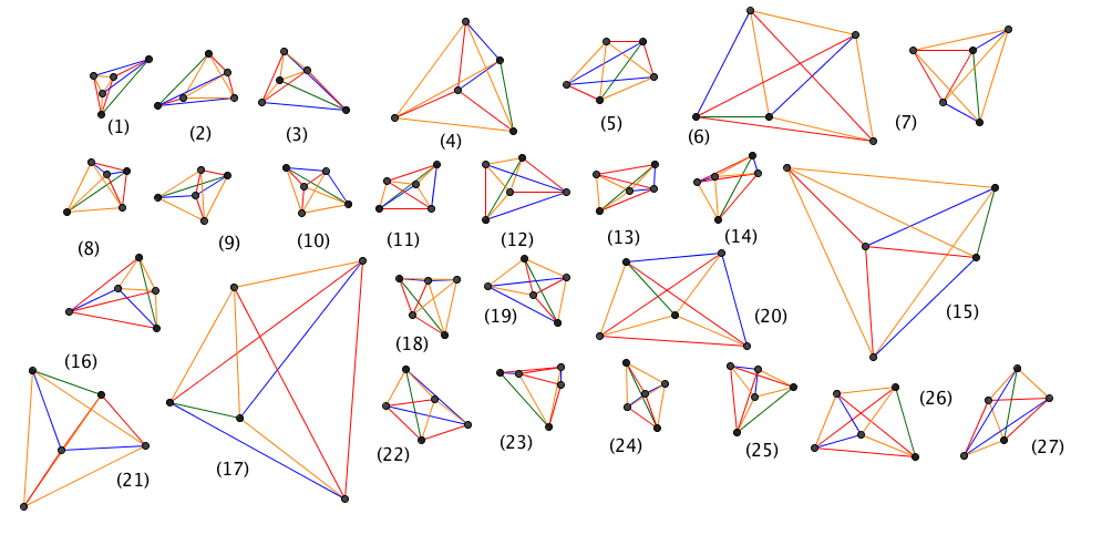
Figure 3. Representatives for all possible crescent configurations on five points.

Remark 1.4.

In Theorem 1.1, we are able to provide an exact number because for all the possible strict distance classes, we were able to give a geometric realizations. However, we are only able to provide a lower bound in 1.3. The reason behind this lie in what the algorithm does both before and after it narrows down to only the strict distance classes. The parallelogram and the isosceles trapezoid have adjacent matrices generated by the same distance class on four points, making such distance class not strict by definition. Any distance class on five points containing the afore-mentioned distance class on four points is therefore not strict, and thrown out at the beginning of the algorithm. Once the strict distance classes are identified, the algorithm tests just one matrix generated by each class, and throws out any class whose corresponding matrix is not geometrically realizable.

The advantage of this algorithmic method is that it can be applied in higher dimensions, though we hope that the running time of $\mathcal{O}(n^{n})$ can still be vastly improved.

In Appendix B we include distance sets and realizable distances for each crescent configuration on four and five points.

In Section 2, we introduce our distance geometry approach and prove a classification of crescent configurations for a general $n$. We follow this in Section 3 with an outline of the first half of the algorithm used to achieve Theorems 1.1 and 1.3. We then move to Section 4 where we discuss how distance geometry methods may be applied to determine whether a distance set is realizable. In Section 5, we outline the second half of the algorithm, completing the proofs for Theorems 1.1 and 1.3. Lastly in Section 6, we discuss potential future work, including improvements to our algorithm as well as extensions to higher number of points and dimensions.

Remark 1.5.

The authors are happy to provide copies of any code referenced in the course of this paper. Please email Steven.Miller.MC.96@aya.yale.edu.

2. Classification of Crescent Configurations

In this section we provide the key definitions and theorems that we use to classify crescent configurations.

Definition 2.1 (General Position [BGMMPS]).

We say that n points are in general position in $\mathbb{R}^{d}$ if no d+1 points lie on the same hyperplane and no d+2 lie on the same hypersphere.

Definition 2.2 (Crescent Configuration [BGMMPS]).

We say $n$ points are in crescent configuration (in $\mathbb{R}^{d}$) if they lie in general position in $\mathbb{R}^{d}$ and determine $n-1$ distinct distances, such that for every $1\leq i\leq n-1$ there is a distance that occurs exactly $i$ times.

The notion of general position is very important in the construction of crescent configurations. Without this notion, the problem of placing $n$ points in $\mathbb{R}^{d}$ to determine $n-1$ distinct distances satisfying the prescribed multiplicities becomes trivial. By simply placing $n$ points on a line in an arithmetic progression, we solve the problem in any dimension.

For now, we keep the following definitions general. In section 3 we will discuss the case in which the mentioned distances are measured with the Euclidean metric.

Definition 2.3 (Distance Coordinate).

The distance coordinate, $D_{A}$, of a point $A$ is the multiset of all distances, counting multiplicity, between $A$ and the other points in a set $\mathcal{P}$. Order does not matter.

Definition 2.4 (Distance Set).

The distance set, $\mathcal{D}$ corresponding to a set of points, $\mathcal{P}$, is the multiset of the distance coordinates for each point in the $\mathcal{P}$.

Definition 2.5 (Distance Class).

Two configurations are said to belong to the same distance class if they possess the same distance set.

Definition 2.6 (Strict Distance Class).

A strict distance class is a distance class in which no elements satisfies one or more of the following criteria:

1. The configuration contains one point at the center of a circle of radius $d_{i}$ with four or more points on this circle as seen in Figure 4.

2. The configuration contains three (or more) isosceles triangles sharing the same base.

3. The configurations contains four points arranged on the vertices of an isosceles trapezoid.

We will discuss this further in the following section.

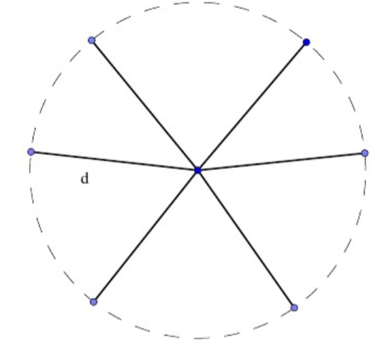
Figure 4. The central point of this configuration has distance coordinate $\{d,d,d,d,d,d\}$.

We note that a crescent configuration on $n$ points can be considered a weighted complete graph with $n-1$ distinct weights associated to the edges in a certain manner, so that the configuration can be realized in $\mathbb{R}^{d}$. The adjacency matrix, thus, is a natural way to store information about the configuration.

The graph isomorphism problem, however, is known to belong to the complexity class NP, with the best currently accepted upper bounds for solving time of $\exp(O(\sqrt{n\log n}))$ due to Babai and Luks [BL]. As such, even if we know that two crescent configurations share the same distance set, it is not obvious, nor necessarily the case, that there exists an isomorphism between them. One example is the following:

$A=\begin{bmatrix}0&3&4&2&4\\ 3&0&4&3&2\\ 4&4&0&4&3\\ 2&3&4&0&1\\ 4&2&3&1&0\\ \end{bmatrix}$             $B=\begin{bmatrix}0&4&4&4&3\\ 4&0&1&3&2\\ 4&1&0&2&3\\ 4&3&2&0&4\\ 3&2&3&4&0\\ \end{bmatrix}$.

Note that there exists a function that maps the vertices of $A$ to the vertices of $B$, defined by $A_{1}\mapsto B_{4}$, $A_{2}\mapsto B_{5}$, $A_{3}\mapsto B_{1}$, $A_{4}\mapsto B_{2}$ and $A_{5}\mapsto B_{3}$. However, the configurations given by these two matrices are not isomorphic as weighted graphs because if they were, $w_{A}(A_{1},A_{2})=w_{B}(B_{4},B_{5})$ but $w_{A}(A_{1},A_{2})=3$ while $w_{B}(B_{4},B_{5})=4$.

That being said, we do now have a tool to encode information of the crescent configuration to some extent. As a result, we will concentrate on determining whether the potential distance sets are realizable, and for each such distance set, finding one crescent configuration corresponding to it.

3. Method for Counting Strict Distance Classes

As a result of the discussion above, we have a way to classify crescent configurations into distance classes using distance sets. We now further refine these to strict distance classes.

In this section we provide a sketch of the algorithm used to find these strict distance classes. A pseudocode is provided in Appendix A.

Remark 3.1.

Since the algorithm can only distinguish the similar permutations according to the distance labels, the resulting distance sets may define crescent configurations that are not geometrically realizable. We address this concern later in the paper (see Section 4 on geometric realizability).

Consider a set of distances, $\{d_{1},d_{2},d_{2},...,d_{n-1}\}$, associated to a crescent configuration on $n$ points. This set of distances may be threaded through an $n\times n$ adjacency matrix.

From this point on, we refer to these matrices as distance matrices; however, they are the equivalent of weighted adjacency matrices in graph theory.

Definition 3.2.

Let $X=\{x_{1},\dots,x_{n}\}$ be a finite metric space with metric $d$. Then the distance matrix corresponding to $X$ is $M=(d_{i,j})$, where the entry $d_{i,j}$ is given by $d(x_{1},x_{j})$.

In our explorations, we are only considering crescent configurations in Euclidean space. Thus, we consider the special case in which $X$ is a finite subset of Euclidean space, and $d$ is the inherited Euclidean distance metric.

Definition 3.3.

A real-valued $n\times n$ matrix $M=(m_{i,j})$ is a Euclidean distance matrix if there exist points $\{x_{1},\dots,x_{n}\}$ such that $m_{i,j}=d(x_{i},x_{j})$, where $d$ is the Euclidean distance metric.

Much of our explorations involve determining whether a given matrix is a Euclidean distance matrix. Thus, we define the following class of candidates for Euclidean distance matrices.

Definition 3.4.

We call a real-valued, square matrix $M\in M_{n}(\mathbb{R})$ a potential distance matrix if it satisfies the following:

1. $M$ is symmetric.

2. All entries off the diagonals are strictly positive.

3. The diagonal entries of $M$ are all $0$.

As each configuration has a distance matrix associated to it, we can generate all possible configurations by threading all permutations of $\{d_{1},d_{2},d_{2},...,d_{n-1}\}$ through potential distance matrices. Using standard combinatorial techniques, we can quickly see that the number of configurations on $n$ points generated by this method is given by

$$\frac{(\frac{n(n-1)}{2})!}{n!(n-1)!\cdots 1!}.$$ (3.1)

This yields 60 configurations on four points, 12,600 on five points, and 37,837,800 on six points. We would now like to further refine our classifications to distance classes using Definition 2.5.

By implementing this restriction, we are able to significantly simplify the problem of identifying realizable crescent configurations. This is especially true for the five point case, as the 12,600 potential configurations may now be approached from a more manageable number, as each distance class can contain no more than 120 different arrangements of the distance set and will actually contain significantly less due to the multiplicities of the distances. It would, in fact, be a very tractable problem to test the realizability of each member of a particular distance class, thus finding all crescent configurations with a given distance set. However, we choose instead to focus on distance classes that do not present any immediate issues with general position. We may then test one member from each for realizability. In doing so, we may then determine a strict lower bound for the number of crescent configurations on $n$ points.

A computer program may then be used to group together all potential distance matrices defining configurations with identical distance sets. These groups then represent our distance classes, and we can conduct the remainder of our analysis on one representative from each class. For $n=4$, this reduces our initial $60$ to $4$ classes. For $n=5$, it reduces our initial $12,600$ to $98$ classes.

Having finished this classification, we must now refine our classes to strict distance classes (see Definition 2.6). Recall that these are distance classes in which every realizable configuration is more likely to obey general position. To see this, we note that there are three degenerate cases specific to $\mathbb{R}^{2}$ that can always be arranged in such a way to force the configuration to violate general position. If none of the elements of a distance class fall into one of these cases, it is called a strict distance class. By restricting ourselves to strict distance classes, we may eliminate entire classes if one representative is proven to be degenerate. This restriction leaves us with 3 potential configurations when $n=4$ (see below for more detail on the 4th case) and 85 potential configurations when $n=5$.

To review from the previous section, the degenerate cases that prevent a distance class from being strict are as follows:

1. The configuration contains one point at the center of a circle of radius $d_{i}$ with four or more points on this circle as seen in Figure 4.

2. The configuration contains three (or more) isosceles triangles sharing the same base.

3. The configurations contains four points arranged on the vertices of an isosceles trapezoid.

Although there exist other cases that will force a class to violate general position, these three cases may be accounted for by only considering the distance matrices.

Case 1 is very simple to account for and is only possible for $n\geq 5$. In order to eliminate these cases, we remove configurations containing one or more distance coordinates in which a particular distance, $d_{i}$, occurs four or more times. In Algorithm A, this case and case 3 are accounted for in the procedure REMOVECYCLIC.

As with case 1, case 2 is only possible for $n\geq 5$. If three or more isosceles triangles share the same base, then all of their apexes must reside on the line bisecting this base, forcing them to violate general position.

In a distance matrix, an isosceles triangle is indicated by a matching pair of distances occurring in a row. Therefore, we remove all potential distance matrices in which three or more rows contain a matching pair occurring in the same slots in each row. This case is accounted for in Algorithm A by the procedure REMOVELINEARCASE.

Case 3 requires us to remove all configurations that contain a subset or subsets of four points defining an isosceles trapezoid, since isosceles trapezoids are always cyclic quadrilaterals.

In Algorithm A, the procedures SUBMATRICES and REMOVECYCLIC are included to account for these cases, which may be identified by their distance matrices using the following lemma.

Lemma 3.5.

A $4\times 4$ distance matrix may be arranged to define an isosceles trapezoid if and only if one of the following holds:

1. the rows of the matrix are generated by permuting the entries of only one row vector such that

   1. the matrix has only two distinct distances, or

   2. the matrix only has three distinct distances,

2. the matrix consists of two distinct rows, and a permutation of each of these two rows such that

   1. the matrix has three distinct distances with multiplicity no greater than three (note that this means each distance occurs no more than six times in the distance matrix), or

   2. the matrix has four distinct distances with multiplicity no greater than two (each distance occurs no more than four times in the distance matrix).

Proof.

($\Leftarrow$) According to Halsted [Hal], a necessary and sufficient condition for a quadrilateral to be an isosceles trapezoid is that it has at least one pair of opposite sides with equal length and diagonals of equal length. It is not possible for these two lengths (sides and diagonals) to be equal because this would create two isosceles triangles that would have to be congruent. Therefore there are three cases for isosceles trapezoids: (1) four distinct distances, (2) three distinct distances, or (3) two distinct distances. Figure 5 presents possible realizations for each of these cases. From here, it is straightforward to show that each of these quadrilaterals satisfies one of the conditions stated in Lemma 3.5, thus completing this direction of the proof.

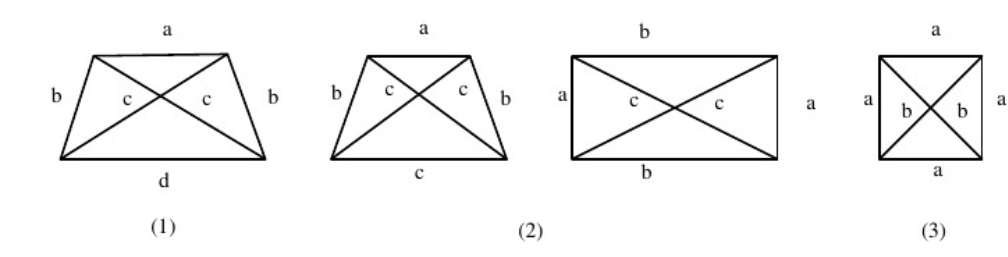
Figure 5. (1) Four distinct distances, (2) three distinct distances, (3) two distinct distances.

($\Rightarrow$) We now prove the other direction.

We begin with condition 1(a): one generating row vector and two distinct distances.

Assume each row represents the distance coordinate $(a,a,b)$ (order of distances may differ among rows). Since we require all rows of the distance matrix to have the same distance coordinate, distance $b$ must touch every point yet only show up twice. Therefore, it must represent both diagonals or two opposite sides. Both cases yield a quadrilateral with a set of congruent opposite sides and congruent diagonals (since we only have two distinct distances), a necessary and sufficient condition for an isosceles trapezoid.

For condition 1(b) - one generating row vector and three distinct distances: all three distances, $(a,b,c)$, must be common to all points. Thus assume the diagonals are not congruent; one has length $a$ and the other length $b$. Then the corner touching the diagonal of length $a$ must be touching a side of length $b$. However, this side also touches the other diagonal, violating the condition of our three distances. If we assume, instead, that we do not have a set of congruent opposite sides, then we inevitably end up with congruent adjacent sides, again violating the condition. Thus, all cases must result in an isosceles trapezoid.

Now we come to condition 2(a) - two distinct rows, each generates another row by permutation, and three distinct distances with multiplicity no greater than three. We note that there are only three types of distance sets we can have: $\{(a,a,a),(a,a,b),(a,b,c)\}$. Since we only have two distinct distance coordinates, if one was of the form $(a,a,a)$, then the distance $a$ would end up occurring five times in the configuration, violating the multiplicity condition.

If one of our distance coordinates has the form $(a,a,b)$, then the other distance set must have the form $(a,b,c)$,$(b,b,c)$, $(b,c,c)$,$(a,a,c)$, or $(a,c,c)$ in order to create three distinct distances. Since we only wish to show that this distance set may be arranged into an isosceles trapezoid, it is enough to find one such arrangement for each example.

We note that each distance cannot occur more than three times, so $(a,a,b)$ can occur at most twice in the distance set, and since $c$ is only found in one of the distinct coordinates, it is clear that it must occur in exactly two distance coordinates. Therefore, if our distinct distance sets are $(a,a,b)$ and $(a,b,c)$, we only need to consider the matrix

$$\begin{pmatrix}0&c&a&b\\ c&0&b&a\\ a&b&0&a\\ b&a&a&0\end{pmatrix}$$ (3.2)

This yields the second configuration shown in figure 5. Clearly this is an isosceles trapezoid, so any configuration in this distance class will likewise be in the same class as an isosceles trapezoid.

If our distinct distance coordinates are $(a,a,b)$ and $(b,b,c)$, however, the double presence of $a$ requires there to be three copies of the coordinate $(a,a,b)$. However, as before, the single presence of the $c$ requires two copies of $(b,b,c)$. We cannot have five distance coordinates for four points, so we reject this case.

A similar argument may be made if our distinct distance coordinates are $(a,a,b)$ and $(b,c,c)$. Furthermore, the coordinates $(a,a,b)$ and $(a,a,c)$ will always result in the distance $a$ having multiplicity 4, so we reject this case as well.

Finally, we reject the case where our coordinates are given by $(a,a,b)$ and $(a,c,c)$ because $b$ must occur in three coordinates and $c$ must occur in three, thus requiring at least five coordinates. Hence the only configuration allowed by condition 2(a) is is one which allows an isosceles trapezoid.

We now end the proof by considering condition 2(b)- two distinct generating rows and four distinct distances with multiplicity no greater than two. We let our distinct distances be $a,b,c,$ and $d$. There are exactly six that may be measured in a set of four points. Thus, if four must be unique and none can occur more than twice, we end up with two distances with multiplicity two and two with multiplicity one. Without loss of generality, we say our distances are $\{a,a,b,b,c,d\}$.

In the upper triangle of an adjacency matrix, each entry represents a side or diagonal of the configuration. If a pair of sides does not share a common end point, then they must represet a pair of opposite sides or diagonals. Thus, in (3.3), the pairs $(a_{12},a_{34})$, $(a_{13},a_{24})$, and $(a_{23},a_{34})$ must represent our pairs of opposite sides and diagonals.

$$\begin{pmatrix}0&a_{12}&a_{13}&a_{14}\\ a_{12}&0&a_{23}&a_{24}\\ a_{13}&a_{23}&0&a_{34}\\ a_{14}&a_{24}&a_{34}&0\end{pmatrix}$$ (3.3)

Again, it is enough to show that just one arrangement of the distances in this case results in an isosceles trapezoid. Indeed, when $a_{13}=a_{24}$ and $a_{23}=a_{14}$ we find that we have two pairs of matching sides/diagonals, so the proof is complete.

∎

Once these cases have been eliminated, we are left with three distance classes for four points and $51$ for five points.

Remark 3.6.

To see that Liu’s configuration is not in a strict distance class, we can look at the adjacency matrix. The adjaency matrix for Liu’s configuration is

$$\begin{pmatrix}0&d2&d1&d3\\ d2&0&d3&d3\\ d1&d3&0&d2\\ d3&d3&d2&0\end{pmatrix}.$$ (3.4)

By applying the row (and column) permutation $1\to 1$, $3\to 2$, $4\to 3$, $2\to 4$, we get the adjacency matrix

$$\begin{pmatrix}0&d1&d3&d2\\ d1&0&d2&d3\\ d3&d2&0&d3\\ d2&d3&d3&0\end{pmatrix},$$ (3.5)

which defines an isosceles trapezoid.

Remark 3.7.

It should be noted that the runtime of Algorithm A is $\mathcal{O}(n^{n})$, so its use is limited to crescent configurations on relatively few points. However, we believe that with enough processing power, upper bounds on the number of strict distance classes can be established using the algorithm for small $n$ such as $7$ and $8$. As such, at this time, this does not pose much of an issue to the progress of this research, as, to the authors’ knowledge, no crescent configuration on more than $8$ points has yet to be found.

4. Geometrically Realizability of Crescent Configurations

In the previous sections we developed a way to find every strict distance class of crescent configurations on $n$ points. However, it is not clear that there exists a set of points in general position in $\mathbb{R}^{m}$ such that the distances between the points correspond to each of these distance set. In this section, we discuss methods of sharpening our previous bounds by taking this consideration into account. In order to determine whether a distance set can be realized as a crescent configuration in $\mathbb{R}^{n}$, we must answer two main questions. First, we must determine whether there exist points in $\mathbb{R}^{m}$ that realize the distance set. We refer to this as geometric realizability. Secondly, we must determine whether such a set of points exist in general position. These two questions turn out to be closely related, and can be answered using similar techniques.

We first set up some framework and introduce some background material. Recall that up to this point, each crescent configuration can be expressed in the form of an $n\times n$ matrix M with the following properties:

• M is a potential distance matrix.

• The multiset of non-diagonal entries is:

  $$\{a_{1},a_{2},a_{2},\dots,a_{n},a_{n},\dots a_{n}\}$$

  where each $a_{i}$ is repeated $i$ times.

We formally define geometric realizability as follows:

Definition 4.1.

A strict distance class for a crescent configuration on $n$ points is geometrically realizable in $\mathbb{R}^{m}$ if there exist some distances $d_{1},\dots,d_{n-1}\in\mathbb{R}_{\geq 0}$ such that setting $a_{i}=d_{i}$ yields a distance set of $n$ points in $R^{m}$.

Remark 4.2.

Burt et. al. [BGMMPS] showed that given an integer $n$, there exists $m$ such that an $n-$crescent configuration exists in $\mathbb{R}^{m}$. In this section, we fix $m$ and determine whether a given distance class is geometrically realizable as a crescent configuration in $\mathbb{R}^{m}$.

Based on our classification system defined previously, we defined geometric realizability in terms of a set of distances between each pair of points. The problem of determining whether a given set of distances can be realized in a space is well-studied, and is known as the distance geometry problem. Thus, we can use techniques from distance geometry in order to sharpen our previous bound on the number of geometrically realizable configurations on $n$ points in $\mathbb{R}^{2}$, and also extend our exploration to higher dimensions. These techniques determine whether a potential distance matrix has a geometric realization. Recall from section 3 that two non-isomorphic potential distance matrices can belong to the same distance class. Thus, in order to completely determine whether a distance set is geometrically realizable, one must use the methods outlined in this section to check every potential distance matrix corresponding to the distance class.

The main tool we use is the Cayley-Menger determinant, which can intuitively be thought of as a way of computing volumes of simplices in Euclidian space.

Definition 4.3.

Consider $M$, an $n\times n$ symmetric matrix of the following form:

$$M=\left(\begin{matrix}0&d_{1,2}&\ldots&d_{1,n}\\ d_{2,1}&0&\ldots&d_{2,n}\\ \vdots&\vdots&\ddots&\vdots\\ d_{n,1}&d_{n,2}&\dots&0\end{matrix}\right),$$

where $d_{i,j}=d_{j,i}$, $d_{i,j}>0$ for all $i,j$. The Cayley-Menger determinant corresponding to $M$, denoted $CM(M)$, is the following determinant:

$$CM(M)=\det\left(\begin{matrix}0&d_{1,2}^{2}&\ldots&d_{1,n}^{2}&1\\ d_{2,1}^{2}&0&\ldots&d_{2,n}^{2}&1\\ \vdots&\vdots&\ddots&\vdots&\vdots\\ d_{n,1}^{2}&d_{n,2}^{2}&\dots&0&1\\ 1&1&\ldots&1&0\end{matrix}\right)$$

The Cayley-Menger determinant can be used to determine whether a given $(n+1)\times(n+1)$ matrix is the distance matrix for a set of points in $\mathbb{R}^{n}$. Failing to adhere to the triangle inequality, for example, could prevent a given matrix from being geometrically realizable as a distance matrix.

Theorem 4.4.

[SS86] Let $M$ be a potential distance matrix. For $2\leq i\leq n+1$, let $M_{i}$ be the minor of $i$ consisting of the first $i$ rows and columns of $M$. Then, $M$ is the distance matrix of $n+1$ points in $\mathbb{R}^{n}$ if and only if $(-1)^{i}CM(M_{i})\geq 0$ for each $i$.

Note that if a $(n+1)\times(n+1)$ matrix is a Euclidean distance matrix, then it must be realizable as the Euclidean distance matrix of points in $\mathbb{R}^{n}$. Thus, the above result can be thought of as a way of identifying obstacles preventing a set of distances to exist in Euclidean space. When considering potential distance matrices of size greater than $n+1$, we must also take into account dimensional constraints in order to determine whether these matrices can be realized as distance matrices for points in $\mathbb{R}^{n}$.

The following result allows us to determine whether a given $(n+2)\times(n+2)$ matrix is the distance matrix for a set of $n+1$ points in $\mathbb{R}^{n}$.

Remark 4.5.

Note: In the following, we use $[n]$ to refer to the set $\{1,2,\dots,n\}.$

Definition 4.6.

Let $M$ be an $n\times n$ potential distance matrix. Let $S\subset[n]$. We define $M_{S}$ to be the minor of $M$ consisting of the rows and columns of $M$ indexed by the elements of $S$.

Theorem 4.7.

[LL] Let $M$ be an $(n+2)\times(n+2)$ potential distance matrix , and suppose $M_{[n+1]}$ can be realized as a distance matrix in $\mathbb{R}^{n}$. Then $M$ can be realized as a Euclidean distance matrix for points in $\mathbb{R}^{n}$ if and only if $CM(M)=0$.

The intuition behind this result comes from the relation between Cayley-Menger determinants and volumes of simplices. The gist of the proof is $CM(M)=0$ roughly means a simplex in $\mathbb{R}^{n+1}$ with the specified lengths has volume $0$, and thus is embeddable in $\mathbb{R}^{n}$.

The following generalization, given by Blumenthal in [B53], gives a complete characterization of whether a given square matrix of size $n>m$ can be expressed nontrivially as the distance matrix of points in $R^{n}$.

Theorem 4.8.

[B53] Let $M$ be an $n\times n$ potential distance matrix. M is the Euclidean distance matrix of a set of $n$ points in $R^{m}$ if and only if:

• There exists a set $S_{0}\subset[n]$ of size $m+1$ such that $CM_{S_{0}}$ satisfies the conditions of 4.4

• For every $S\subset[n]$ of size $m+2$ or $m+3$ such that $S_{0}\subset S$, $CM(M_{S})=0$.

Thus far, we have focused on techniques that tell us whether a given matrix is geometrically realizable in some given dimension. However, in order for a potential distance set to correspond to a valid crescent configuration, it must also have a geometric realization that is in general position.

Recall that in order for a crescent configuration to lie in general position in $\mathbb{R}^{m}$, it must satisfy the following properties:

1. No $m+1$ points lie on the same hyperplane.

2. No $m+2$ points lie on the same hypersphere.

As we have seen above, the Cayley-Menger determinant can be used to determine whether the first condition holds. A similar determinant can be used to determine whether the second condition holds:

Definition 4.9.

Consider $M$, an $n\times n$ symmetric matrix of the following form:

$$M=\left(\begin{matrix}0&d_{1,2}&\ldots&d_{1,n}\\ d_{2,1}&0&\ldots&d_{2,n}\\ \vdots&\vdots&\ddots&\vdots\\ d_{n,1}&d_{n,2}&\dots&0\end{matrix}\right),$$

where $d_{i,j}=d_{j,i}$, $d_{i,j}>0$ for all $i,j$. The Euclidean distance determinant of M, denoted $ED(M)$, is given by the following determinant:

$$ED(M)=\det\left(\begin{matrix}0&d_{1,2}^{2}&\ldots&d_{1,n}^{2}\\ d_{2,1}^{2}&0&\ldots&d_{2,n}^{2}\\ \vdots&\vdots&\ddots&\vdots&\vdots\\ d_{n,1}^{2}&d_{n,2}^{2}&\dots&0\end{matrix}\right).$$

Theorem 4.10.

[DS] Let $M$ be the distance matrix corresponding to points $P_{1},\dots P_{n+2}$ in Euclidean space. These points lie on a hypersphere in $\mathbb{R}^{n}$ if and only if $ED(M)=0$.

The following corollary follows directly from 4.8 and 4.10, and gives a complete characterization as to when a given symmetric matrix can be realized as a distance matrix for points in general position.

Corollary 4.11.

Let $M$ be an $n\times n$ potential distance matrix. Then $M$ is a Euclidean distance matrix for points in $\mathbb{R}^{m}$ in general position if and only if the following conditions hold.

1. There exists $S\subset[n]$ of size $m+1$ such that $M_{S_{0}}$ can be realized as the distance matrix of $m+1$ points in $R^{m+1}$.

2. For every $S$ of size $m+2$ or $m+3$ containing $S_{0}$, $CM(M_{S})=0$.

3. For every $S$ of size $m+1$, $CM(M_{S})\neq 0$.

4. For every $S$ of size $m+2$, $ED(M_{S})\neq 0$.

In turns out that we can adjust this slightly by dropping the stipulation that we only consider $S$ of size $m+2$ or $m+3$ if $S$ contains $S_{0}$, by using the following special case of theorem 4.8:

Theorem 4.12.

[B53] Let $M$ be a real $(n+3)\times(n+3)$ potential distance matrix. Suppose that there is some $S_{0}\subset[n]$ of size $n+1$ such that $M_{S_{0}}$ is the distance matrix of $n+1$ linearly independent points in $R^{n}$. Then $M$ is the distance matrix of a set of $n+3$ points in $R_{n}$ if and only if:

1. For the two subsets $S$ of size $n+2$ containing $S_{0}$, $CM(M_{S})=0$.

2. $CM(M)=0$.

We use the above theorem to establish the following version of the corollary:

Corollary 4.13.

Let $M$ be a $n\times n$ potential distance matrix. Then $M$ is a Euclidean distance matrix for points in $\mathbb{R}^{m}$ in general position if and only if the following conditions hold.

1. There exists $S\subset[n]$ of size $m+1$ such that $M_{S_{0}}$ can be realized as the distance matrix of $m+1$ points in $R^{m+1}$.

2. For every $S$ of size $m+2$ or $m+3$, $CM(M_{S})=0$.

3. For every $S$ of size $m+1$, $CM(S)\neq 0$.

4. For every $S$ of size $m+2$, $ED(S)\neq 0$.

Proof.

$(\rightarrow)$ Suppose $M$ is geometrically realizable in general position in $\mathbb{R}^{m}$. It suffices to show that for every $S$ of size $m+2$ or $m+3$, $CM(M_{S})=0$. Consider some $S\subset[n]$ of size $m+3$. $S$ must contain some $S_{0}$ of size $m+1$. Since $M$ is realizable as a distance matrix for points in $\mathbb{R}^{m}$, so must $M_{S}$ and $M_{S_{0}}$, since the extra points can just be removed. Furthermore, $M_{S_{0}}$ is the distance matrix of a set of $m+1$ points that form a linearly independent set in $R^{m}$, since $M$ is a distance matrix for points in general position. From 4.12, we see that this implies $CM(M_{s})=0$, and for $S^{\prime}$ of size $m+2$ such that $S\subset S^{\prime}\subset S$, $CM(M_{S^{\prime}})=0$. Since $S$ was chosen arbitrarily, we see that all subsets of size $m+2,m+3$ must correspond to a Cayley-Menger determinant of 0.

$(\leftarrow)$ If $M$ satisfies the conditions (1), (2), and (3), then it certainly satisfies the conditions of 4.11 and thus is geometrically realizable in general position in $\mathbb{R}^{m}$. ∎

Our application of 4.13 to the distance sets on $4$ and $5$ points have allowed us to find a lower bound for the geometric realizability of each of the distance sets found using techniques from earlier sections. These geometrically realizable configurations are discussed in the following section.

Thus far, most of our attentions have been focused on crescent configurations in the plane. However, these techniques can be applied to finding crescent configurations in higher dimensions, furthering the work of Burt et. al. [BGMMPS].

5. Finding Geometric Realizations for Crescent Configurations

As stated in Section 3, Algorithm A yields three potential distance matrices on four points and 51 on five points, each corresponding to a different strict distance class. However, these procedures do not guarantee that these potential distance matrices are geometrically realizable. Furthermore, for each strict distance class, our algorithm only found one potential distance matrix. It is possible that others may exist.

To check which of these matrices are geometrically realizable, we run Algorithm A. A pseudocode of this algorithm can be found in Appendix A. Note that we assume $d_{1}=1$ in order to simplify the procedure.

Algorithm A is an extended application of Theorem 4.11 and Corrollary 4.13. The first step of this algorithm is to take the Cayley-Menger determinants of all $4$-point and $5$-point subsets of each potential distance matrix found by Algorithm A and set them equal to zero. Doing so yields a system of $\begin{pmatrix}n\\ 4\end{pmatrix}$ equations with unknowns : $\{d_{2},d_{3},...,d_{n-1}\}$. If the configuration is realizable in the plane, solving this system of equations will give all possible solutions to these distances in $\mathbb{R}^{2}$. Note that the values must be positive and real-valued.

For each of these solutions, we check the Cayley-Menger determinants of all $3$-point subsets of the configuration. If one or more of these determinants equals zero, that solution forces the configuration to place three points on the same line, violating general position. In such case, we discard it. If none of the determinants are zero, we keep the solution.

For each remaining solution, we take the determinant of the Euclidean distance matrix of each $4$-point subset of the configuration. If any of these determinants equal zero, the solution forces four points onto the same circle, violating general position, and we throw it away.

Finally, we verify that Theorem 4.4 is satisfied. To do this, we check the Cayley-Menger determinants of each 2-point and 3-point subset and verify that their determinants are equal to $(-1)^{2}$ an $(-1)^{3}$, respectively. Any remaining solutions represent the distances of a geometrically realizable crescent configuration.

Applying this algorithm to the potential distance matrices returned by Algorithm A completes the proofs of Theorems 1.1 and 1.3, as we find that there are at least three realizable crescent configurations on four points and 27 realizable crescent configurations on five points. Note that in the five point case, this is a lower bound since we only tested one potential distance matrix corresponding to each distance class. It is possible that the matrix we tested was not realizable, but a different matrix corresponding to the same distance class is realizable. For the four point case, we do not have this problem. Since every strict distance class was found to have an element that is geometrically realizable, we know that there are exactly three realizable strict classes of crescent configurations on four points.

In Appendix B, we provide a set of distances for every configuration on five points that had at least one remaining solution after applying this algorithm.

6. Future Work

6.1. Improving the Algorithm

As mentioned in 1, the algorithm we introduce currently gets rid of any configuration containing Liu’s legal parallelogram subgraph [Liu]. This is due to the fact that though the parallelogram itself does not violate general position, it is isomorphic to a configuration that does. For configurations on four points, we were able to go back and recover such configuration, which is just the parallelogram itself. This improves the classification compared to Liu’s result, and gives a procedure for how to obtain the most complete profile. Inevitably, adding such feature will certainly add a layer to the complexity of the program. It is thus an important open task to characterize configurations containing a legal parallelogram.
Moreover, we currently only sample one matrix from each strict distance class to test geometric realizability. As pointed out earlier in the paper, one distance class could generate adjacency matrices which corresponds to non-isomorphic configurations. Thus to obtain a sharper result, it is necessary to further divide the matrices generated by the same strict distance class into equivalence classes via isomorphism. Once this is achieved, we would be able to test one representative from each class to recover the lost configurations.

6.2. Further Explorations in the Plane

Thus far, we have used our techniques to classify crescent configurations in the plane for $n=4$ and $n=5$. Because of the complexity of our algorithm, we have not been able to apply our techniques to higher $n$. As mentioned above, the runtime of our current algorithm is on the order of $n^{n}$, which prevents us from carrying out this process for large $n$. However, so far no configurations have been found for $n>8$, so even running a similar algorithm for $n=9$ would yield significant progress on this problem. Thus, we are interested in the possibility of modifying our algorithm, or finding a new technique that would allow us to count crescent configurations on higher $n$. In this way, we could develop a sequence of $\{c_{i}\}$, where each $c_{i}$ gives the number of crescent configurations on $i$ points. If Erdős’ conjecture is correct, then $\{c_{i}\}$ only has a finite number of non-zero terms. It would be interesting to see Erdős’ conjecture realized as a sequence that goes to zero.

Since our techniques yield one crescent configuration for each possible distance class for a given $n$, we can use these to observe patterns. For example, one can see from Figure 3 that many of crescent configurations on 5 points contain crescent configurations on 4 points. We may be able to develop techniques using such patterns that generate some of the possible crescent configurations for larger $n$.

6.3. Extensions to Higher Dimensions

As mentioned earlier, the distance geometry techniques that we use naturally extend to higher dimensions. Thus, we are interested in using these techniques to find the number of crescent configurations on $n$ points in a given dimension. Our goal is to construct a sequence for each $d$ consisting of the number of crescent configurations on $i$ points in $\mathbb{R}^{d}$ for each $i$. Currently, constructions in $\mathbb{R}^{3}$ have been found for 3, 4, and 5 points. Thus, even finding a single 6 point configuration in 3D would give new information. We have attempted to use techniques from distance geometry to find a realization in $\mathbb{R}^{3}$ of a known distance set for $n=6$ in the plane. However, the resulting systems of equations exceeded our computational resources.

Recently, Burt et. al [BGMMPS] found that given $d$ high enough, one can always construct a crescent configuration on $n$ points in $\mathbb{R}^{d}$. We can consider similar questions using the concept of distance coordinates. We are interested in determining whether given a distance set there always exists a dimension in which the set is geometrically realizable.

6.4. Properties of Crescent Configuration Types

Now that we have developed a way of classifying crescent configurations, we can examine certain properties for each of the types of crescent configurations.
One property that we started exploring but needs further work is the rigidity of crescent configurations. A graph is rigid when its vertices cannot be continuously moved to non-congruent positions while preserving all its distances. A more precise definition can be found in Asimov and Roth [AR]. A rigid graph could be redundantly rigid if any of its vertices could be removed and the remaining graph is rigid. While studying the result we presented in this paper, we learned that crescent configurations are all rigid owing to Laman’s Theorem [Lam] and the fact that they are complete graphs. However, we want to study further if, and for which value of $n$, one distance set could define two different realisations of crescent configurations belonging to the same distance class. The rigidity testing of these configurations would not only serve as a verification of our classification under distance class, but would also give us another way to characterize these crescent configurations.

Another direction we are interested in is to develop a concept of stability for these configurations. This is due to our observation that moving the points of the M, R, and C- type configurations resulted in different levels of change in the distances. Further, should we define two distances to be equal if they are $\epsilon$ apart, then our combined study of the stability and rigidity of crescent configurations could have some powerful applications to the study of molecules.

Appendix A

Below we include pseudocode for Algorithms A and A.

CrescentClassificationdistances,n Permutationsdistances data  all  permutations  of  distances
data AdjacencyMatrixdistances,n w ∈Permutationsdistances Thread  the  list  through  an  n ×n  matrix  to  create  a  symmetric  matrix  with  diagonal  $0$. ReOrderdistances,n x ∈AdjacencyMatrixdistances,n Sort  the  elements  of  each  row  into  canonical  order,  then  sort  the  rows  by  first  element. RemoveDuplicatesdistances,n i ∈ReOrderdistances,n $i=0$ Delete  i Delete  all  duplicates  of  i,  keeping  only  first  instance. Check  all  4-point  subsets  for  isosceles  trapezoids
SubMatricesdistances, n y ∈RemoveDuplicatesdistances,n k Take  all   4 ×4  submatrices  taken
along  the  diagonal.
k RemoveCyclicdistances, n z ∈RemoveDuplicatsdistances,n No  i ∈SubMatricesdistances,n  defines  a  cyclic  quadrilateral  or  circle z 0 RemoveLinearCasedistances,n z ∈RemoveCyclicdistances,n ∃ 3  or  more  isosceles  triangles  sharing  the  same  base 0 z

CrescentClassificationContinueddistances,n FinalFormdistances,n j ∈RemoveDuplicatesdistances, n AdjacencyMatrixdistances, n. (x,y) (distances,n)
FinalFormx,y

GeometryCheckdistances, n SubMatricesdistances, n y ∈CrescentClassificationdistances,n k Take  all   4 ×4  submatrices  taken
along  the  diagonal.
k CayleyMengerdistances,n k ∈SubMatricesdistances,n S Take  Cayley-Menger  determinants  of  each  4 ×4  and  5 × 5  submatrix  and  set
equal  to  zero
S This  generates  the  system  of  equations  used  to  solve  for  {d_2,d_3,…,d_n}.
SolutionsCheckdistances,n S ∈CayleyMengerdistances,n {d_2,d_3,…,d_n} Solution  for  S.
{d_2,d_3,…,d_n} ⊂(0,∞) CrescentClassificationdistances,n NULL
TriangleInequalitydistances,n A  ∈  SolutionsCheckdistances,n S Take  Cayley-Menger  determinants  of each  2 ×2   submatrix
T Take  Cayley-Menger  determinants  of each  3 ×3   submatrix
y  ≠ (-1)^2  ∈ S  ||  z  ≠ (-1)^3  ∈ T NULL A This  verifies  that  the  triangle  inequality  is  satisfied. LineCheckdistances,n y  ∈ CayleyMengerdistances,n y Set  of  Cayley-Menger  determinants  of  all
3 ×3  submatrices  of  y  taken  along  the  diagonal
0  in  y NULL SolutionsCheckdistances,n By  4.8,  the  Cayley-Menger  determinant  of  a  3×3  matrix
will  indicate  if  the  three  points  lie  on  the  same  line.

GeometryCheckContinueddistances,n

EuclideanDistanceMatrixdistances,n f x^2 y ∈LineCheckdistances,n k Map  f  to  each  element  of  y
k

The  next  procedure  is  a  direct  application  of  Theorem  4.10.
CircleCheckdistances,n k  ∈ EuclideanDistanceMatrixdistances,n j the  set  of  determinants  of  all  4×4  submatrices  taken  along  the  diagonal  of  k
0  ∈ j NULL SolutionsCheckdistances,n (x,y) (distances,n) CircleCheckx,y

Appendix B

Below we provide a list of adjacency matrices and distances for each configuration shown in Figures 2 and 3. These represent members from all possible distance classes of configurations on four and five points. We say $d1=1$ for all configurations on five points.

Note that most of these solutions are irrational and many of them have no nice form (we consider $\frac{1}{\sqrt{2}}$ and $\sqrt{1-\sqrt{3}}$ to be nice forms). In these cases, numerical values are provided up to four decimal places. Contact the author for a list of Mathematica outputs.

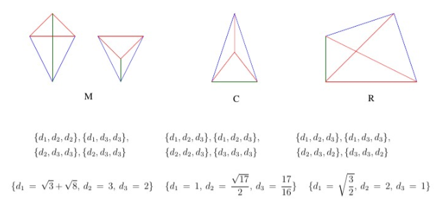
Figure 6. Types M, C, and R with distance coordinates and values.

Table 1. Representative distance matrices for all 27 distance classes of crescent configurations on five points.

Distance Matrices for Five Points
$(1)\ \begin{pmatrix}0&1&d_{2}&d_{2}&d_{3}\\ 1&0&d_{3}&d_{4}&d_{4}\\ d_{2}&d_{3}&0&d_{4}&d_{4}\\ d_{2}&d_{4}&d_{4}&0&d_{4}\\ d_{3}&d_{3}&d_{4}&d_{4}&0\end{pmatrix}$	$(2)\ \begin{pmatrix}0&1&d_{2}&d_{2}&d_{3}\\ 1&0&d_{3}&d_{4}&d_{4}\\ d_{2}&d_{3}&0&d_{3}&d_{4}\\ d_{2}&d_{4}&d_{3}&0&d_{4}\\ d_{3}&d_{4}&d_{4}&d_{4}&0\end{pmatrix}$	$(3)\ \begin{pmatrix}0&1&d_{2}&d_{2}&d_{3}\\ 1&0&d_{4}&d_{4}&d_{4}\\ d_{2}&d_{4}&0&d_{3}&d_{3}\\ d_{2}&d_{4}&d_{3}&0&d_{4}\\ d_{3}&d_{4}&d_{3}&d_{4}&0\end{pmatrix}$
$(4)\ \begin{pmatrix}0&1&d_{2}&d_{2}&d_{4}\\ 1&0&d_{3}&d_{4}&d_{4}\\ d_{2}&d_{3}&0&d_{3}&d_{3}\\ d_{2}&d_{4}&d_{3}&0&d_{4}\\ d_{4}&d_{4}&d_{3}&d_{4}&0\end{pmatrix}$	$(5)\ \begin{pmatrix}0&1&d_{2}&d_{3}&d_{3}\\ 1&0&d_{3}&d_{4}&d_{4}\\ d_{2}&d_{3}&0&d_{2}&d_{4}\\ d_{3}&d_{4}&d_{2}&0&d_{4}\\ d_{3}&d_{4}&d_{4}&d_{4}&0\end{pmatrix}$	$(6)\ \begin{pmatrix}0&1&d_{2}&d_{3}&d_{3}\\ 1&0&d_{4}&d_{2}&d_{4}\\ d_{2}&d_{4}&0&d_{2}&d_{3}\\ d_{3}&d_{2}&d_{4}&0&d_{4}\\ d_{3}&d_{4}&d_{3}&d_{4}&0\end{pmatrix}$
$(7)\ \begin{pmatrix}0&1&d_{3}&d_{2}&d_{3}\\ 1&0&d_{2}&d_{4}&d_{4}\\ d_{3}&d_{2}&0&d_{4}&d_{3}\\ d_{2}&d_{4}&d_{4}&0&d_{4}\\ d_{3}&d_{4}&d_{3}&d_{4}&0\end{pmatrix}$	$(8)\ \begin{pmatrix}0&1&d_{2}&d_{3}&d_{3}\\ 1&0&d_{4}&d_{4}&d_{4}\\ d_{2}&d_{4}&0&d_{2}&d_{3}\\ d_{3}&d_{4}&d_{2}&0&d_{4}\\ d_{3}&d_{4}&d_{3}&d_{4}&0\end{pmatrix}$	$(9)\ \begin{pmatrix}0&1&d_{2}&d_{3}&d_{4}\\ 1&0&d_{2}&d_{4}&d_{4}\\ d_{2}&d_{2}&0&d_{3}&d_{3}\\ d_{3}&d_{4}&d_{3}&0&d_{4}\\ d_{4}&d_{4}&d_{3}&d_{4}&0\end{pmatrix}$
$(10)\ \begin{pmatrix}0&1&d_{2}&d_{3}&d_{4}\\ 1&0&d_{2}&d_{4}&d_{4}\\ d_{2}&d_{2}&0&d_{3}&d_{4}\\ d_{3}&d_{4}&d_{3}&0&d_{3}\\ d_{4}&d_{4}&d_{4}&d_{3}&0\end{pmatrix}$	$(11)\ \begin{pmatrix}0&1&d_{2}&d_{4}&d_{3}\\ 1&0&d_{3}&d_{2}&d_{4}\\ d_{2}&d_{3}&0&d_{4}&d_{3}\\ d_{4}&d_{2}&d_{4}&0&d_{4}\\ d_{3}&d_{4}&d_{3}&d_{4}&0\end{pmatrix}$	$(12)\ \begin{pmatrix}0&1&d_{2}&d_{3}&d_{4}\\ 1&0&d_{3}&d_{4}&d_{4}\\ d_{2}&d_{3}&0&d_{2}&d_{3}\\ d_{3}&d_{4}&d_{2}&0&d_{4}\\ d_{4}&d_{4}&d_{3}&d_{4}&0\end{pmatrix}$
$(13)\ \begin{pmatrix}0&1&d_{2}&d_{4}&d_{3}\\ 1&0&d_{3}&d_{4}&d_{4}\\ d_{2}&d_{3}&0&d_{2}&d_{3}\\ d_{4}&d_{4}&d_{2}&0&d_{4}\\ d_{3}&d_{4}&d_{3}&d_{4}&0\end{pmatrix}$	$(14)\ \begin{pmatrix}0&1&d_{2}&d_{3}&d_{4}\\ 1&0&d_{3}&d_{4}&d_{4}\\ d_{2}&d_{3}&0&d_{3}&d_{4}\\ d_{3}&d_{4}&d_{3}&0&d_{2}\\ d_{4}&d_{4}&d_{4}&d_{2}&0\end{pmatrix}$	$(15)\ \begin{pmatrix}0&1&d_{3}&d_{2}&d_{4}\\ 1&0&d_{2}&d_{4}&d_{4}\\ d_{3}&d_{2}&0&d_{3}&d_{3}\\ d_{2}&d_{4}&d_{3}&0&d_{4}\\ d_{4}&d_{4}&d_{3}&d_{4}&0\end{pmatrix}$
$(16)\ \begin{pmatrix}0&1&d_{2}&d_{3}&d_{4}\\ 1&0&d_{4}&d_{3}&d_{4}\\ d_{2}&d_{4}&0&d_{2}&d_{4}\\ d_{3}&d_{3}&d_{2}&0&d_{3}\\ d_{4}&d_{4}&d_{4}&d_{3}&0\end{pmatrix}$	$(17)\ \begin{pmatrix}0&1&d_{2}&d_{3}&d_{4}\\ 1&0&d_{4}&d_{2}&d_{4}\\ d_{2}&d_{4}&0&d_{3}&d_{3}\\ d_{3}&d_{2}&d_{3}&0&d_{4}\\ d_{4}&d_{4}&d_{3}&d_{4}&0\end{pmatrix}$	$(18)\ \begin{pmatrix}0&1&d_{2}&d_{4}&d_{3}\\ 1&0&d_{4}&d_{4}&d_{3}\\ d_{2}&d_{4}&0&d_{2}&d_{3}\\ d_{4}&d_{4}&d_{2}&0&d_{4}\\ d_{3}&d_{3}&d_{3}&d_{4}&0\end{pmatrix}$
$(19)\ \begin{pmatrix}0&1&d_{2}&d_{4}&d_{3}\\ 1&0&d_{4}&d_{4}&d_{3}\\ d_{2}&d_{4}&0&d_{2}&d_{4}\\ d_{4}&d_{4}&d_{2}&0&d_{3}\\ d_{3}&d_{3}&d_{4}&d_{3}&0\end{pmatrix}$	$(20)\ \begin{pmatrix}0&1&d_{2}&d_{3}&d_{4}\\ 1&0&d_{4}&d_{4}&d_{4}\\ d_{2}&d_{4}&0&d_{2}&d_{3}\\ d_{3}&d_{4}&d_{2}&0&d_{3}\\ d_{4}&d_{4}&d_{3}&d_{3}&0\end{pmatrix}$	$(21)\ \begin{pmatrix}0&1&d_{2}&d_{4}&d_{4}\\ 1&0&d_{3}&d_{3}&d_{4}\\ d_{2}&d_{3}&0&d_{2}&d_{3}\\ d_{4}&d_{3}&d_{2}&0&d_{4}\\ d_{4}&d_{4}&d_{3}&d_{4}&0\end{pmatrix}$
$(22)\ \begin{pmatrix}0&1&d_{2}&d_{4}&d_{4}\\ 1&0&d_{3}&d_{3}&d_{4}\\ d_{2}&d_{3}&0&d_{2}&d_{4}\\ d_{4}&d_{3}&d_{2}&0&d_{3}\\ d_{4}&d_{4}&d_{4}&d_{3}&0\end{pmatrix}$	$(23)\ \begin{pmatrix}0&1&d_{2}&d_{4}&d_{4}\\ 1&0&d_{4}&d_{3}&d_{4}\\ d_{2}&d_{4}&0&d_{3}&d_{3}\\ d_{4}&d_{3}&d_{3}&0&d_{2}\\ d_{4}&d_{4}&d_{3}&d_{2}&0\end{pmatrix}$	$(24)\ \begin{pmatrix}0&1&d_{3}&d_{3}&d_{4}\\ 1&0&d_{3}&d_{4}&d_{4}\\ d_{3}&d_{3}&0&d_{2}&d_{2}\\ d_{3}&d_{4}&d_{2}&0&d_{4}\\ d_{4}&d_{4}&d_{2}&d_{4}&0\end{pmatrix}$
$(25)\ \begin{pmatrix}0&1&d_{3}&d_{3}&d_{4}\\ 1&0&d_{4}&d_{3}&d_{4}\\ d_{3}&d_{4}&0&d_{2}&d_{2}\\ d_{3}&d_{3}&d_{2}&0&d_{4}\\ d_{4}&d_{4}&d_{2}&d_{4}&0\end{pmatrix}$	$(26)\ \begin{pmatrix}0&1&d_{4}&d_{3}&d_{3}\\ 1&0&d_{4}&d_{3}&d_{4}\\ d_{4}&d_{4}&0&d_{2}&d_{2}\\ d_{3}&d_{3}&d_{2}&0&d_{4}\\ d_{3}&d_{4}&d_{2}&d_{4}&0\end{pmatrix}$	$(27)\ \begin{pmatrix}0&1&d_{2}&d_{4}&d_{4}\\ 1&0&d_{4}&d_{3}&d_{4}\\ d_{2}&d_{4}&0&d_{2}&d_{3}\\ d_{4}&d_{3}&d_{2}&0&d_{3}\\ d_{4}&d_{4}&d_{3}&d_{3}&0\end{pmatrix}$

Table 2. Realizable distances for each matrix in Table LABEL:tab:_matrixTABLE.

Realizable Distances for Five Points
(1)	$\ \{d_{2}\to\sqrt{\frac{6-3\sqrt{2}-\sqrt{6(3-2\sqrt{2})}}{2(2-\sqrt{2})}},\ d_{3}\to\sqrt{\frac{2-\sqrt{2}}{2}},\ d_{4}\to\sqrt{\frac{4-2\sqrt{2}-\sqrt{6(3-2\sqrt{2})}}{2}}\}$
(2)	$\ \{d_{2}\to\sqrt{\frac{4-\sqrt{3}}{2}},\ d_{3}\to\sqrt{\frac{2-\sqrt{3}}{2}},\ d_{4}\to\frac{1}{\sqrt{2}}\}$
(3)	$\ \{d_{2}\to\sqrt{\frac{1+\sqrt{3}}{2}},\ d_{3}\to\frac{1}{2}(-1+\sqrt{3+2\sqrt{3}}),\ d_{4}\to\frac{1}{2}\sqrt{2-2\sqrt{-3+2\sqrt{3}}}\}$
(4)	$\ \{d_{2}\to 1.2091,\ d_{3}\to 0.5028,\ d_{4}\to 0.8135\}$
(5)	$\ \{d_{2}\to\frac{1}{2}\sqrt{\frac{13+\sqrt{73}}{2}},\ d_{3}\to\frac{1}{2}\sqrt{\frac{23+3\sqrt{73}}{2}},\ d_{4}\to\frac{1}{2}\sqrt{\frac{9+\sqrt{73}}{2}}\}$
(6)	$\ \{d_{2}\to\frac{1}{\sqrt{2}},\ d_{3}\to\sqrt{\frac{3+\sqrt{6}}{6}},\ d_{4}\to\sqrt{\frac{3}{2}+\sqrt{\frac{3}{2}}}\}$
(7)	$\ \{d_{2}\to\frac{1}{\sqrt{3}},\ d_{3}\to\sqrt{\frac{2}{3}},\ d_{4}\to\sqrt{1+\sqrt{\frac{2}{3}}}\}$
(10)	$\ \{d_{2}\to 0.2757,\ d_{3}\to 0.5107,\ d_{4}\to 0.7621\}$
(9)	$\ \{d_{2}\to\sqrt{2-\sqrt{3}},\ d_{3}\to\sqrt{\frac{2-\sqrt{3}}{2}},\ d_{4}\to\frac{1}{\sqrt{2}}\}$
(10)	$\ \{d_{2}\to\sqrt{\frac{2(4-\sqrt{13})}{-1+\sqrt{13}}},\ d_{3}\to\sqrt{\frac{4-\sqrt{13}}{3}},\ d_{4}\to\sqrt{\frac{-1+\sqrt{13}}{6}}\}$
(11)	$\ \{d_{2}\to\sqrt{\frac{-35+19\sqrt{13}}{17(9-\sqrt{13})}},\ d_{3}\to\sqrt{\frac{9-\sqrt{13}}{34}},\ d_{4}\to\sqrt{\frac{9-\sqrt{13}}{34}}\}$
(12)	$\ \{d_{2}\to\sqrt{\frac{1+\sqrt{3}}{2}},\ d_{3}\to\frac{-1+\sqrt{3+2\sqrt{3}}}{2},\ d_{4}\to\frac{1}{\sqrt{2+3^{\frac{1}{4}}\sqrt{2}}}\}$
(13)	$\ \{d_{2}\to 0.3383,\ d_{3}\to 0.8135,\ d_{4}\to 0.5028\}$
(14)	$\ \{d_{2}\to\sqrt{8-3\sqrt{7}},\ d_{3}\to\sqrt{\frac{2(45-17\sqrt{7})}{8-3\sqrt{7}}},\ d_{4}\to\sqrt{3-\sqrt{7}}\}$
(15)	$\ \{d_{2}\to 1.9696,\ d_{3}\to 1.5321,\ d_{4}\to 2.8794\}$
(16)	$\ \{d_{2}\to 0.7597,\ d_{3}\to 1.2293,\ d_{4}\to 0.5112\}$
(17)	$\ \{d_{2}\to\sqrt{4+\sqrt{13}},\ d_{3}\to\frac{1}{2}(3+\sqrt{13}),\ d_{4}\to\sqrt{\frac{1}{2}(3+\sqrt{13})}\}$
(18)	$\ \{d_{2}\to 0.3976,\ d_{3}\to 0.5304,\ d_{4}\to 0.7944\}$
(19)	$\ \{d_{2}\to 1.0879,\ d_{3}\to 0.5154,\ d_{4}\to 0.6344\}$
(20)	$\ \{d_{2}\to 1.3275,\ d_{3}\to 2.0277,\ d_{4}\to 1.0730\}$
(21)	$\ \{d_{2}\to 1.1578,\ d_{3}\to 0.9345,\ d_{4}\to 1.8686\}$
(22)	$\ \{d_{2}\to 1.1561,\ d_{3}\to 0.6707,\ d_{4}\to 0.5801\}$
(23)	$\ \{d_{2}\to\sqrt{8-3\sqrt{7}},\ d_{3}\to\sqrt{\frac{45-17\sqrt{7}}{8-3\sqrt{7}}},\ d_{4}\to\sqrt{2\frac{45-17\sqrt{7}}{8-3\sqrt{7}}}\}$
(24)	$\ \{d_{2}\to 0.3107,\ d_{3}\to 0.5028,\ d_{4}\to 0.6180\}$
(25)	$\ \{d_{2}\to\frac{\sqrt{4-\sqrt{7}}}{3},\ d_{3}\to\frac{1}{3}\sqrt{\frac{13-\sqrt{7}}{4-\sqrt{7}}},\ d_{4}\to\frac{1}{3}(-1+\sqrt{7})\}$
(26)	$\ \{d_{2}\to 0.6599,\ d_{3}\to 1.3930,\ d_{4}\to 0.8124\}$
(27)	$\ \{d_{2}\to\sqrt{2},\ d_{3}\to\sqrt{2(3-\sqrt{7})},\ d_{4}\to\sqrt{3-\sqrt{7}}\}$

References

- [AR] L. Asimow and B. Roth, "The Rigidity of Graphs", Trans. Amer. Math. Soc., 245 (1978),279–289.
- [BGMMPS] D. Burt, E. Goldstein, S. Manski, S.J. Miller, E.A. Palsson and H. Suh, "Crescent Configurations", Integers, 16 (2016), #A38. arXiv:1509.07220.
- [BL] L. Babai, E. M. Luks, ”Canonical Labeling of Graphs”, Proceedings of the Fifteenth Annual ACM Symposium on Theory of Computing, (1983), 171–183.
- [B53] L.M. Blumenthal, "Theory and Applications of Distance Geometry", Clarendon Press, 1953.
- [DS] C. D’Andrea, M. Sombra, "The Cayley-Menger determinant is irreducible for all ", Siberian Journal of Mathematics, 46 (2005), 46–71.
- [Erd46] P. Erdős, "On sets of distances of points", Amer. Math. Monthly, 53 (1946), 248–250.
- [Erd89] P. Erdős, "Distances with specified multiplicities", Amer. Math. Monthly, 96 (1989), 447.
- [Erd96] P. Erdős, "On some of my favourite theorems", Combinatorics, Paul Erdős is Eighty, Vol. 2 (D. Miklós et al., eds.), Bolyai Society Mathematical Studies 2, Budapest, 1996, 97–132.
- [GK] L.Guth and N.H.Katz, "On the Erdős distinct distances problem in the plane", Annals of Mathematics, 181 (2015), 155–190.
- [Hal] G. B. Halsted, Elementary Synthetic Geometry, J. Wiley and Sons (1896), 50–53.
- [HHH] S. Hsieh, C. Hsu and L. Hsu, "Efficient Method to Perform Isomorphism Testing of Labelled Graphs", Computational Science and its Aplications– ICCSA 2006: International Conference, Glasgow, UK, May 8-11, 2006, Proceedings, Part 5 (M. Gavrilova, et al, eds.), Springer, 2006, 422–431.
- [Lam] G. Laman, "On graphs and rigidity of plane skeletal structures", J. Eng. Math., 4 (1970), 331–340.
- [Liu] A. Liu, "On the "seven points problem" of P. Erdős", New Zealand Journal of Mathematics, 15 (1986), 29–33.
- [LL] L. Liberti, C. Lavor, "Six mathematical gems from the history of distance geometry.", International Transactions in Operational Research, 23 (2016), 897–920.
- [Pal87] I. Palásti, "On the seven points problem of P. Erdős", Stud. Sci. Math. Hungar., 22 (1987), 447–448.
- [Pal89] I. Palásti, "Lattice point examples for a question of Erdős", Period. Math. Hungar., 20 (1989), 231–235.
- [She] A. Sheffer, "Distinct Distances: Open Problems and Current Bounds", (2015). arXiv:1406.1949.
- [SS86] M.J. Sipple, H.A. Scheraga, "Cayley-menger coordinates", Proceedings of the National Academy of Sciences, 83 no. 8 (1986), 2283–2287.