Generalization Bounds for Weighted Automata

Abstract

This paper studies the problem of learning weighted automata from a finite labeled training sample. We consider several general families of weighted automata defined in terms of three different measures: the norm of an automaton’s weights, the norm of the function computed by an automaton, or the norm of the corresponding Hankel matrix. We present new data-dependent generalization guarantees for learning weighted automata expressed in terms of the Rademacher complexity of these families. We further present upper bounds on these Rademacher complexities, which reveal key new data-dependent terms related to the complexity of learning weighted automata.

1 Introduction

Weighted finite automata (WFAs) provide a general and highly expressive framework for representing functions mapping strings to real numbers. The mathematical theory behind WFAs, that of rational power series, has been extensively studied in the past [28, 53, 38, 14] and has been more recently the topic of a dedicated handbook [25]. WFAs are widely used in modern applications, perhaps most prominently in image processing and speech recognition where the terminology of weighted automata seems to have been first introduced and made popular [32, 46, 51, 44, 48], in several other speech processing applications such as speech synthesis [54, 2], in phonological and morphological rule compilation [34, 35, 50], in parsing [47], machine translation [23], bioinformatics [27, 3], sequence modeling and prediction [21], formal verification and model checking [5, 4], in optical character recognition [17], and in many other areas.

The recent developments in spectral learning [31, 6] have triggered a renewed interest in the use of WFAs in machine learning, with several recent successes in natural language processing [8, 9] and reinforcement learning [16, 30]. The interest in spectral learning algorithms for WFAs is driven by the many appealing theoretical properties of such algorithms, which include their polynomial-time complexity, the absence of local minima, statistical consistency, and finite sample bounds à la PAC [31]. However, the typical statistical guarantees given for the hypotheses used in spectral learning only hold in the realizable case. That is, these analyses assume that the labeled data received by the algorithm is sampled from some unknown WFA. While this assumption is a reasonable starting point for theoretical analyses, the results obtained in this setting fail to explain the good performance of spectral algorithms in many practical applications where the data is typically not generated by a WFA. See [11] for a recent survey of algorithms for learning WFAs with a discussion of the different assumptions and learning models.

There exists of course a vast literature in statistical learning theory providing tools to analyze generalization guarantees for different hypothesis classes in classification, regression, and other learning tasks. These guarantees typically hold in an agnostic setting where the data is drawn i.i.d. from an arbitrary distribution. For spectral learning of WFAs, an algorithm-dependent agnostic generalization bound was proven in [10] using a stability argument. This seems to have been the first analysis to provide statistical guarantees for learning WFAs in an agnostic setting. However, while [10] proposed a broad family of algorithms for learning WFAs parametrized by several choices of loss functions and regularizations, their bounds hold only for one particular algorithm within this family.

In this paper, we start the systematic development of algorithm-independent generalization bounds for learning with WFAs, which apply to all the algorithms proposed in [10], as well as to others using WFAs as their hypothesis class. Our approach consists of providing upper bounds on the Rademacher complexity of general classes of WFAs. The use of Rademacher complexity to derive generalization bounds is standard [37] (see also [13] and [49]). It has been successfully used to derive statistical guarantees for classification, regression, kernel learning, ranking, and many other machine learning tasks (e.g. see [49] and references therein). A key benefit of Rademacher complexity analyses is that the resulting generalization bounds are data-dependent.

Our main results consist of upper bounds on the Rademacher complexity of three broad classes of WFAs. The main difference between these classes is the quantities used for their definition: the norm of the transition weight matrix or initial and final weight vectors of a WFA; the norm of the function computed by a WFA; and, the norm of the Hankel matrix associated to the function computed by a WFA. The formal definitions of these classes is given in Section 3. Let us point out that our analysis of the Rademacher complexity of the class of WFAs described in terms of Hankel matrices directly yields theoretical guarantees for a variety of spectral learning algorithms. We will return to this point when discussing the application of our results. As an application of our Rademacher complexity bounds we provide a variety of generalizations bounds for learning with WFAs using a bounded Lipschitz loss function; our bounds include both data-dependent and data-independent bounds.

Related Work.

To the best of our knowledge, this paper is the first to provide general tools for deriving learning guarantees for broad classes of WFAs. However, there exists some related work providing complexity bounds for some sub-classes of WFAs in agnostic settings. The VC-dimension of deterministic finite automata (DFAs) with $n$ states over an alphabet of size $k$ was shown by [33] to be in $O(kn\log n)$. This can be used to show that the Rademacher complexity of this class of DFA is bounded by $O(\sqrt{nk\log n/m})$. For probabilistic finite automata (PFAs), it was shown by [1] that, in an agnostic setting, a sample of size $\widetilde{O}(kT^{2}n^{2}/\varepsilon^{2})$ is sufficient to learn a PFA with $n$ states and $k$ symbols whose log-loss error is at most $\varepsilon$ away from the optimal one in the class when the error is measured on all strings of length $T$. New learning bounds on the Rademacher complexity of DFAs and PFAs follow as straightforward corollaries of the general results we present in this paper.

Another recent line of work, which aims to provide guarantees for spectral learning of WFAs in the non-realizable setting, is the so-called low-rank spectral learning approach [40]. This has led to interesting upper bounds on the approximation error between minimal WFAs of different sizes [39]. See [12] for a polynomial-time algorithm for computing these approximations. This approach, however, is more limited than ours for two reasons. First, because it is algorithm-dependent. And second, because it assumes that the data is actually drawn from some (probabilistic) WFA, albeit one that is larger than any of the WFAs in the hypothesis class considered by the algorithm.

The rest of this paper is organized as follows. Section 2 introduces the notation and technical concepts used throughout. Section 3 describes the three classes of WFAs for which we provide Rademacher complexity bounds. The bounds are formally stated and proven in Sections 4, 5, and 6. In Section 7 we provide additional bounds required for converting some sample-dependent bounds from Sections 5 and 6 into sample-independent bounds. Finally, the generalizations bounds obtained using the machinery developed in previous sections are given in Section 8.

2 Preliminaries

2.1 Weighted Automata, Rational Functions, and Hankel Matrices

Let $\Sigma$ be a finite alphabet of size $k$. Let $\epsilon$ denote the empty string and $\Sigma^{\star}$ the set of all finite strings over the alphabet $\Sigma$. The length of $u\in\Sigma^{\star}$ is denoted by $|u|$. Given an integer $L\geq 0$, we denote by $\Sigma^{\leq L}$ the set of all strings with length at most $L$: $\Sigma^{\leq L}=\{x\in\Sigma^{\star}\colon|x|\leq L\}$. Given two strings $u,v\in\Sigma^{\star}$ we write $uv$ for their concatenation.

A WFA over the alphabet $\Sigma$ with $n\geq 1$ states is a tuple $A=\langle\boldsymbol{\alpha},\boldsymbol{\beta},\{\mathbf{A}_{a}\}_{a\in\Sigma}\rangle$ where $\boldsymbol{\alpha},\boldsymbol{\beta}\in\mathbb{R}^{n}$ are the initial and final weights, and $\mathbf{A}_{a}\in\mathbb{R}^{n\times n}$ the transition matrix whose entries give the weights of the transitions labeled with $a$. Every WFA $A$ defines a function $f_{A}\colon\Sigma^{\star}\to\mathbb{R}$ defined for all $x=a_{1}\cdots a_{t}\in\Sigma^{\star}$ by

$$f_{A}(x)=f_{A}(a_{1}\cdots a_{t})=\boldsymbol{\alpha}^{\top}\mathbf{A}_{a_{1}}\cdots\mathbf{A}_{a_{t}}\boldsymbol{\beta}=\boldsymbol{\alpha}^{\top}\mathbf{A}_{x}\boldsymbol{\beta}\enspace,$$ (1)

where $\mathbf{A}_{x}=\mathbf{A}_{a_{1}}\cdots\mathbf{A}_{a_{t}}$. This algebraic expression in fact corresponds to summing the weights of all possible paths in the automaton indexed by the symbols in $x$, where the weight of a single path $(q_{0},q_{1},\ldots,q_{t})\in[n]^{t+1}$ is obtained by multiplying the initial weight of $q_{0}$, the weights of all transitions from $q_{s-1}$ to $q_{s}$ labeled by $x_{s}$, and the final weight if state $q_{t}$. That is:

$$f_{A}(x)=\sum_{(q_{0},\ldots,q_{t})\in[n]^{t+1}}\boldsymbol{\alpha}(q_{0})\left(\prod_{s=1}^{t}\mathbf{A}_{x_{s}}(q_{s-1},q_{s})\right)\boldsymbol{\beta}(q_{t})\enspace.$$

See Figure 1 for an example of WFA with $3$ states given in terms of its algebraic representation and the equivalent representation as a weighted transition diagram between states.

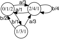
(a)

$\boldsymbol{\alpha}=\left[\begin{matrix}1\\ 3\\ 4\\ \end{matrix}\right]$	$\mathbf{A}_{a}=\left[\begin{matrix}0&0&3\\ 0&0&3\\ 1&0&0\\ \end{matrix}\right]$
$\boldsymbol{\beta}=\left[\begin{matrix}2\\ 1\\ 1\\ \end{matrix}\right]$	$\mathbf{A}_{b}=\left[\begin{matrix}0&1&0\\ 2&0&0\\ 0&0&4\\ \end{matrix}\right]$

(b)

Figure 1: (1(a)) Example of WFA $A$. Within each circle, the first number indicates the state number, the second after the slash separator the initial weight and the third the final weight. In particular, $f_{A}(ab)=1\times 3\times 4\times 1+3\times 3\times 4\times 1+4\times 1\times 1\times 1$. (1(b)) Corresponding initial vector $\boldsymbol{\alpha}$, final vector $\boldsymbol{\beta}$, and transition matrices $\mathbf{A}_{a}$ and $\mathbf{A}_{b}$.

An arbitrary function $f\colon\Sigma^{\star}\to\mathbb{R}$ is said to be rational if there exists a WFA $A$ such that $f=f_{A}$. The rank of $f$ is denoted by $\operatorname{rank}(f)$ and is defined as the minimal number of states of a WFA $A$ such that $f=f_{A}$. Note that minimal WFAs are not unique. In fact, it is not hard to see that, for any minimal WFA $A=\langle\boldsymbol{\alpha},\boldsymbol{\beta},\{\mathbf{A}_{a}\}\rangle$ with $f=f_{A}$ and any invertible matrix $\mathbf{Q}\in\mathbb{R}^{n\times n}$, $A^{\mathbf{Q}}=\langle\mathbf{Q}^{\top}\boldsymbol{\alpha},\mathbf{Q}^{-1}\boldsymbol{\beta},\{\mathbf{Q}^{-1}\mathbf{A}_{a}\mathbf{Q}\}\rangle$ is also another minimal WFA computing $f$. We sometimes write $A(x)$ instead of $f_{A}(x)$ to emphasize the fact that we are considering a specific parametrization of $f_{A}$. Note that for the purpose of this paper we only consider weighted automata over the familiar field of real numbers with standard addition and multiplication (see [28, 53, 15, 38, 45] for more general definitions of WFAs over arbitrary semirings). Functions mapping strings to real numbers can also be viewed as non-commutative formal power series, which often helps deriving rigorous proofs in formal language theory [53, 15, 38]. We will not favor that point of view here, however, since we will not need to make explicit mention of the algebraic properties offered by that perspective.

An alternative method to represent rational functions independently of any WFA parametrization is via their Hankel matrices. The Hankel matrix $\mathbf{H}_{f}\in\mathbb{R}^{\Sigma^{\star}\times\Sigma^{\star}}$ of a function $f\colon\Sigma^{\star}\to\mathbb{R}$ is the infinite matrix with rows and columns indexed by all strings with $\mathbf{H}_{f}(u,v)=f(uv)$ for all $u,v\in\Sigma^{\star}$. By the theorem of Fliess [29] (see also [18] and [15]), $\mathbf{H}_{f}$ has finite rank $n$ if and only if $f$ is rational and there exists a WFA $A$ with $n$ states computing $f$, that is, $\operatorname{rank}(f)=\operatorname{rank}(\mathbf{H}_{f})$.

2.2 Learning Scenario

Let $\mathcal{Z}$ denote a measurable subset of $\mathbb{R}$. We assume a standard supervised learning scenario where training and test points are drawn i.i.d. according to some unknown distribution $D$ over $\Sigma^{\star}\times\mathbb{R}$.

Let $\mathcal{F}$ be a subset of the family of functions mapping from $\mathcal{X}$ to $\mathcal{Y}$, with $\mathcal{Y}\subseteq\mathbb{R}$, and let $\ell\colon\mathcal{Y}\times\mathcal{Z}\to\mathbb{R}_{+}$ be a loss function measuring the divergence between the prediction $y\in\mathcal{Y}$ made by a function in $\mathcal{F}$ and the target label $z\in\mathcal{Z}$. The learner’s objective consists of using a labeled training sample $S=((x_{1},z_{1}),\ldots,(x_{m},z_{m}))$ of size $m$ to select a function $f\in\mathcal{F}$ with small expected loss, that is

$$\mathfrak{L}_{D}(f)=\operatorname*{\mathbb{E}}_{(x,z)\sim D}[\ell(f(x),z)]\enspace.$$

Our objective is to derive learning guarantees for broad families of weighted automata or rational functions used as hypothesis sets in learning algorithms. To do so, we will derive upper bounds on the Rademacher complexity of different classes of rational functions $f\colon\Sigma^{\star}\to\mathbb{R}$. Thus, we start with a brief introduction to the main definitions and results regarding the Rademacher complexity of an arbitrary class of functions $\mathcal{F}=\{f\colon\mathcal{X}\to\mathcal{Y}\}$ where $\mathcal{X}$ is the input space and $\mathcal{Y}\subseteq\mathbb{R}$ the output space. Let $D$ be a probability distribution over $\mathcal{X}\times\mathcal{Z}$ for some $\mathcal{Z}\subseteq\mathbb{R}$ and denote by $D_{\mathcal{X}}$ the marginal distribution over $\mathcal{X}$. Suppose $S=(x_{1},\ldots,x_{m})\stackrel{{\scriptstyle\text{iid}}}{{\sim}}D_{\mathcal{X}}^{m}$ is a sample of $m$ i.i.d. examples drawn from $D$. The empirical Rademacher complexity of $\mathcal{F}$ on $S$ is defined as follows:

$$\widehat{\mathfrak{R}}_{S}(\mathcal{F})=\operatorname*{\mathbb{E}}\left[\sup_{f\in\mathcal{F}}\frac{1}{m}\sum_{i=1}^{m}\sigma_{i}f(x_{i})\right]\enspace,$$

where the expectation is taken over the $m$ independent Rademacher random variables $\sigma_{i}\sim\mathbf{Unif}(\{+1,-1\})$. The Rademacher complexity of $\mathcal{F}$ is defined as the expectation of $\widehat{\mathfrak{R}}_{S}(\mathcal{F})$ over the draw of a sample $S$ of size $m$:

$$\mathfrak{R}_{m}(\mathcal{F})=\operatorname*{\mathbb{E}}_{S\sim D_{\mathcal{X}}^{m}}\left[\widehat{\mathfrak{R}}_{S}(\mathcal{F})\right]\enspace.$$

The Rademacher complexity of a hypothesis class can be used to derive generalization bounds for a variety of learning tasks [37, 13, 49]. To do so, we need to bound the Rademacher complexity of the associated loss class, for a given loss function $\ell\colon\mathcal{Y}\times\mathcal{Z}\to\mathbb{R}_{+}$.

For a given hypothesis class $\mathcal{F}$ the corresponding loss class $\ell\circ\mathcal{F}$ is given by the set of all functions $\ell\circ f\colon\mathcal{X}\times\mathcal{Z}\to\mathbb{R}_{+}$ of the form $(x,z)\mapsto\ell(f(x),z)$. By Talagrand’s contraction lemma [41], the empirical Rademacher complexity of $\ell\circ\mathcal{F}$ can be bounded in terms of $\widehat{\mathfrak{R}}_{S}(\mathcal{F})$, when $\ell$ is $\mu$-Lipschitz with respect to its first argument for some $\mu>0$, that is when

$$|\ell(y,z)-\ell(y^{\prime},z)|\leq\mu|y-y^{\prime}|$$

for all $y,y^{\prime}\in\mathcal{Y}$ and $z\in\mathcal{Z}$. In that case, the following inequality holds: $\widehat{\mathfrak{R}}_{S^{\prime}}(\ell\circ\mathcal{F})\leq\mu\widehat{\mathfrak{R}}_{S}(\mathcal{F})$, where $S^{\prime}=((x_{1},z_{1}),\ldots,(x_{m},z_{m}))$ is a sample of size $m$ with $(x_{i},z_{i})\in\mathcal{X}\times\mathcal{Z}$ and $S=(x_{1},\ldots,x_{m})$ denotes the sample of elements in $\mathcal{X}$ obtained from $S^{\prime}$. When taking expectations over $S^{\prime}\stackrel{{\scriptstyle\text{iid}}}{{\sim}}D^{m}$ and $S\stackrel{{\scriptstyle\text{iid}}}{{\sim}}D_{\mathcal{X}}^{m}$ we obtain the same bound for the Rademacher complexities $\mathfrak{R}_{m}(\ell\circ\mathcal{F})\leq\mu\mathfrak{R}_{m}(\mathcal{F})$. A typical example of a loss function that is $\mu$-Lipschitz with respect to its first argument is the absolute loss $\ell(y,z)=|y-z|$, which satisfies the condition with $\mu=1$ for $\mathcal{Y}=\mathcal{Z}=\mathbb{R}$.

3 Classes of Rational Functions

In this section we introduce several classes of rational functions. Each of these classes is defined in terms of a different way to measure the complexity of rational functions. The first one is based on the weights of an explicit WFA representation, while the other two are based on intrinsic quantities associated to the function: the norm of the function, and the norm of the corresponding Hankel matrix when viewed as a linear operator on a certain Hilbert space. These three points of view measure different aspects of the complexity of a rational function, and each of them provides distinct benefits in the analysis of learning with WFAs. The Rademacher complexity of each of these classes will be analyzed in Sections 4, 5, and 6.

3.1 The Class $\mathcal{A}_{n,p,r}$

We start by considering the case where each rational function is given by a fixed WFA representation. Our learning bounds would then naturally depend on the number of states and the weights of the WFA representations.

Fix an integer $n>0$ and let $\mathcal{A}_{n}$ denote the set of all WFAs with $n$ states. Note that any $A\in\mathcal{A}_{n}$ is identified by the $d=n(kn+2)$ parameters required to specify its initial, final, and transition weights. Thus, we can identify $\mathcal{A}_{n}$ with the vector space $\mathbb{R}^{d}$ by suitably defining addition and scalar multiplication. In particular, given $A,A^{\prime}\in\mathcal{A}_{n}$ and $c\in\mathbb{R}$, we define:

$$A+A^{\prime} =\langle\boldsymbol{\alpha},\boldsymbol{\beta},\{\mathbf{A}_{a}\}\rangle+\langle\boldsymbol{\alpha}^{\prime},\boldsymbol{\beta}^{\prime},\{\mathbf{A}_{a}^{\prime}\}\rangle=\langle\boldsymbol{\alpha}+\boldsymbol{\alpha}^{\prime},\boldsymbol{\beta}+\boldsymbol{\beta}^{\prime},\{\mathbf{A}_{a}+\mathbf{A}_{a}^{\prime}\}\rangle$$

$$cA =c\langle\boldsymbol{\alpha},\boldsymbol{\beta},\{\mathbf{A}_{a}\}\rangle=\langle c\boldsymbol{\alpha},c\boldsymbol{\beta},\{c\mathbf{A}_{a}\}\rangle\enspace.$$

We can view $\mathcal{A}_{n}$ as a normed vector space by endowing it with any norm from the following family. Let $p,q\in[1,+\infty]$ be Hölder conjugates, i.e. $p^{-1}+q^{-1}=1$. It is easy to check that the following defines a norm on $\mathcal{A}_{n}$:

$$\|A\|_{p,q}=\max\left\{\|\boldsymbol{\alpha}\|_{p},\|\boldsymbol{\beta}\|_{q},\max_{a}\|\mathbf{A}_{a}\|_{q}\right\}\enspace,$$

where $\|\mathbf{A}\|_{q}$ denotes the matrix norm induced by the corresponding vector norm, that is $\|\mathbf{A}\|_{q}=\sup_{\|\mathbf{v}\|_{q}=1}\|\mathbf{A}\mathbf{v}\|_{q}$. Given $p\in[1,+\infty]$ and $q=1/(1-1/p)$, we denote by $\mathcal{A}_{n,p,r}$ the set of all WFAs $A$ with $n$ states and $\|A\|_{p,q}\leq r$. Thus, $\mathcal{A}_{n,p,r}$ is the ball of radius $r$ at the origin in the normed vector space $(\mathcal{A}_{n},\|\cdot\|_{p,q})$.

3.1.1 Examples

We consider first the class of deterministic finite automata (DFA). A DFA can be represented by a WFA where: $\boldsymbol{\alpha}$ is the indicator vector of the initial state; the entries of $\boldsymbol{\beta}$ are values in $\{0,1\}$ indicating whether a state is accepting or rejecting; and, for any $a\in\Sigma$ and any $i\in[n]$ we have that the $i$th row of $A_{a}$ is either the all zero vector if there is no transition from the $i$th state labeled by $a$, or an indicator vector with a one on the $j$th position if taking an $a$-transition from state $i$ leads to state $j$. Therefore, a DFA $A=\langle\boldsymbol{\alpha},\boldsymbol{\beta},\{\mathbf{A}_{a}\}\rangle$ satisfies $\|A\|_{1,\infty}\leq 1$ and $\mathcal{A}_{n,1,1}$ contains all DFA with $n$ states.

Another important class of WFA contained in $\mathcal{A}_{n,1,1}$ is that of probabilistic finite automata (PFA). To represent a PFA as a WFA we consider automata where: $\boldsymbol{\alpha}$ is a probability distribution over possible initial states; the vector $\boldsymbol{\beta}$ contains stopping probabilities for every state; and for every $a\in\Sigma$ and $i,j\in[n]$ the entry $\mathbf{A}_{a}(i,j)$ represents the probability of transitioning from state $i$ to state $j$ while outputting the symbol $a$. Any WFA satisfying these constraints clearly has $\|\boldsymbol{\alpha}\|_{1}=1$, $\|\boldsymbol{\beta}\|_{\infty}\leq 1$, and $\|\mathbf{A}_{a}\|_{\infty}=\max_{i}\sum_{j}|\mathbf{A}_{a}(i,j)|\leq 1$. The function $f_{A}$ computed by a PFA $A$ defines a probability distribution over $\Sigma^{\star}$; i.e. we have $f_{A}(x)\geq 0$ for all $x\in\Sigma^{\star}$ and $\sum_{x\in\Sigma^{\star}}f_{A}(x)=1$.

3.2 The Class $\mathcal{R}_{p,r}$

Next, we consider an alternative quantity measuring the complexity of rational functions that is independent of any WFA representation: their norm. Given $p\in[1,\infty]$ and $f\colon\Sigma^{\star}\to\mathbb{R}$ we use $\|f\|_{p}$ to denote the $p$-norm of $f$ given by

$$\|f\|_{p}=\bigg{[}\sum_{x\in\Sigma^{\star}}|f(x)|^{p}\bigg{]}^{\frac{1}{p}}\enspace,$$

which in the case $p=\infty$ amounts to $\|f\|_{\infty}=\sup_{x\in\Sigma^{\star}}|f(x)|$.

Let $\mathcal{R}_{p}$ denote the class of rational functions with finite $p$-norm: $f\in\mathcal{R}_{p}$ if and only if $f$ is rational and $\|f\|_{p}<+\infty$. Given some $r>0$ we also define $\mathcal{R}_{p,r}$, the class of functions with $p$-norm bounded by $r$:

$$\mathcal{R}_{p,r}=\left\{f\colon\Sigma^{\star}\to\mathbb{R}\mid f\text{ rational and }\|f\|_{p}\leq r\right\}\enspace.$$

Note that this definition is independent of the WFA used to represent $f$.

3.2.1 Examples and Membership Testing

If $A$ is a PFA, then the function $f_{A}$ is a probability distribution and we have $f_{A}\in\mathcal{R}_{1,1}$ and by extension $\mathcal{R}_{p,1}$ for all $p\in[1,+\infty]$. On the other hand, if $A$ is a DFA such that $f_{A}(x)=1$ for infinitely many $x\in\Sigma^{\star}$, then $f_{A}\in\mathcal{R}_{\infty,1}$, but $f_{A}\notin\mathcal{R}_{p}$ for any $p<+\infty$. In fact, it is easy to see that for any $n\geq 0$ we have $\mathcal{A}_{n,1,1}\subseteq\mathcal{R}_{\infty}$. These examples show that $\mathcal{A}_{n,1,1}\cap\mathcal{R}_{1}\neq\emptyset$ and $\mathcal{A}_{n,1,1}\cap(\mathcal{R}_{\infty}\setminus\mathcal{R}_{1})\neq\emptyset$. Thus, the classes $\mathcal{R}_{p}$ yield a more fine grained characterization of the complexity of rational functions than what the classes $\mathcal{A}_{n,p,r}$ can provide in general.

However, while testing membership of a WFA in $\mathcal{A}_{n,p,r}$ is a straightforward task, testing membership in any of the $\mathcal{R}_{p}$ can be challenging. Membership in $\mathcal{R}_{1,r}$ was shown to be semi-decidable in [7]. On the other hand, membership in $\mathcal{R}_{2,r}$ can be decided in polynomial time [22]. The inclusion $\mathcal{A}_{n,1,1}\subseteq\mathcal{R}_{\infty}$ gives an easy to test sufficient condition for membership in $\mathcal{R}_{\infty}$.

3.3 The Class $\mathcal{H}_{p,r}$

Here, we introduce a third class of rational functions described via their Hankel matrices, a quantity that is also independent of their WFA representations. To do so, we represent a function $f$ using its Hankel matrix $\mathbf{H}_{f}$, interpret this matrix as a linear operator on a Hilbert space contained in the free vector space $\mathbb{R}^{\Sigma^{\star}}$, and consider the Schatten $p$-norm of $\mathbf{H}_{f}$ as a measure of complexity of $f$. To make this more precise we start by noting that the set

$$\mathcal{L}_{2}=\left\{f\colon\Sigma^{\star}\to\mathbb{R}\mid\|f\|_{2}<\infty\right\}$$

together with the inner product $\left<f,g\right>=\sum_{x\in\Sigma^{\star}}f(x)g(x)$ forms a separable Hilbert space. Note we have the obvious inclusion $\mathcal{R}_{2}\subset\mathcal{L}_{2}$, but not all functions in $\mathcal{L}_{2}$ are rational. Given an arbitrary function $f\colon\Sigma^{\star}\to\mathbb{R}$ we identify the Hankel matrix $\mathbf{H}_{f}$ with a (possibly unbounded) linear operator $\mathbf{H}_{f}\colon\mathcal{L}_{2}\to\mathcal{L}_{2}$ defined by

$$(\mathbf{H}_{f}g)(x)=\sum_{y\in\Sigma^{\star}}f(xy)g(y)\enspace.$$

Recall that an operator $\mathbf{H}_{f}$ is bounded when its operator norm is finite; i.e. $\|\mathbf{H}_{f}\|=\sup_{\|g\|_{2}\leq 1}\|\mathbf{H}_{f}g\|_{2}<\infty$. Furthermore, a bounded operator is compact if it can be obtained as the limit of a sequence of bounded finite-rank operators under an adequate notion of convergence. In particular, bounded finite-rank operators are compact. Our interest in compact operators on Hilbert spaces stems from the fact that these are precisely the operators for which a notion equivalent to the SVD for finite matrices can be defined. Thus, if $f$ is a rational function of rank $n$ such that $\mathbf{H}_{f}$ is bounded (note this implies compactness by Fliess’ theorem), then we can use the singular values $\mathfrak{s}_{1}\geq\ldots\geq\mathfrak{s}_{n}$ of $\mathbf{H}_{f}$ as a measure of the complexity of $f$. The following result follows from [12] and gives a useful condition for the boundedness of $\mathbf{H}_{f}$.

Lemma 1.

Suppose the function $f\colon\Sigma^{\star}\to\mathbb{R}$ is rational. Then $\mathbf{H}_{f}$ is bounded if and only if $\|f\|_{2}<\infty$.

We see that every Hankel matrix $\mathbf{H}_{f}$ with $f\in\mathcal{R}_{2}$ has a well-defined SVD. Therefore, for any $f\in\mathcal{R}_{2}$ it makes sense to define its Schatten–Hankel $p$-norm as the Schatten $p$-norm of its Hankel matrix: $\|f\|_{\mathrm{H},p}=\|\mathbf{H}_{f}\|_{\mathrm{S},p}=\|(\mathfrak{s}_{1},\ldots,\mathfrak{s}_{n})\|_{p}$, where $\mathfrak{s}_{i}=\mathfrak{s}_{i}(\mathbf{H}_{f})$ is the $i$th singular value of $\mathbf{H}_{f}$ and $\operatorname{rank}(\mathbf{H}_{f})=n$. Using this notation, we can define several classes of rational functions. For a given $p\in[1,+\infty]$, we denote by $\mathcal{H}_{p}$ the class of rational functions with $\|f\|_{\mathrm{H},p}<\infty$ and, for any $r>0$, we write $\mathcal{H}_{p,r}$ the for class of rational functions with $\|f\|_{\mathrm{H},p}\leq r$.

Note that the discussion above implies $\mathcal{H}_{p}=\mathcal{R}_{2}$ for every $p\in[1,+\infty]$, and therefore we can see the classes $\mathcal{H}_{p,r}$ as providing an alternative stratification of $\mathcal{R}_{2}$ than the classes $\mathcal{R}_{2,r}$. As a consequence of this containment we also have $\mathcal{R}_{1}\subset\mathcal{H}_{p}$ for every $p$, and therefore the classes $\mathcal{H}_{p}$ include all functions computed by probabilistic automata. Since membership in $\mathcal{R}_{2}$ is efficiently testable [22], a polynomial time algorithm from [12] can be used to compute $\|f\|_{\mathrm{H},p}$ and thus test membership in $\mathcal{H}_{p,r}$.

4 Rademacher Complexity of $\mathcal{A}_{n,p,r}$

In this section, we present an upper bound on the Rademacher complexity of the class of WFAs $\mathcal{A}_{n,p,r}$. To bound $\mathfrak{R}_{m}(\mathcal{A}_{n,p,r})$, we will use an argument based on covering numbers. We first introduce some notation, then state our general bound and related corollaries, and finally prove the main result of this section.

Let $S=(x_{1},\ldots,x_{m})\in\left(\Sigma^{\star}\right)^{m}$ be a sample of $m$ strings with maximum length $L_{S}=\max_{i}|x_{i}|$. The expectation of this quantity over a sample of $m$ strings drawn i.i.d. from some fixed distribution $D$ will be denoted by $L_{m}=\operatorname*{\mathbb{E}}_{S\sim D^{m}}[L_{S}]$. It is interesting at this point to note that $L_{m}$ appears in our bound and introduces a dependency on the distribution $D$ which will exhibit different growth rates depending on the behavior of the tails of $D$. For example, it is well known that if the random variable $|x|$ for $x\sim D$ is sub-Gaussian, then $L_{m}=O(\sqrt{\log m})$. Similarly, if the tail of $D$ is sub-exponential, then $L_{m}=O(\log m)$ and if the tail is a power-law with exponent $s+1$, $s>0$, then $L_{m}=O(m^{1/s})$. Note that in the latter case the distribution of $|x|$ has finite variance if and only if $s>1$.

Theorem 2.

The following inequality holds for every sample $S\in(\Sigma^{\star})^{m}$:

$$\widehat{\mathfrak{R}}_{S}(\mathcal{A}_{n,p,r})\leq\inf_{\eta>0}\left(\eta+r^{L_{S}+2}\sqrt{\frac{2n(kn+2)\log\Big{(}2r+\frac{r^{L_{S}+2}(L_{S}+2)}{\eta}\Big{)}}{m}}\right)\enspace.$$

By considering the case $r=1$ and choosing $\eta=(L_{S}+2)/m$ we obtain the following corollary.

Corollary 3.

For any $m\geq 1$ and $n\geq 1$ the following inequalities holds:

$$\mathfrak{R}_{m}(\mathcal{A}_{n,p,1}) \leq\sqrt{\frac{2n(kn+2)\log(m+2)}{m}}+\frac{L_{m}+2}{m}\enspace,$$

$$\widehat{\mathfrak{R}}_{S}(\mathcal{A}_{n,p,1}) \leq\sqrt{\frac{2n(kn+2)\log(m+2)}{m}}+\frac{L_{S}+2}{m}\enspace.$$

4.1 Proof of Theorem 2

We begin the proof by recalling several well-known facts and definitions related to covering numbers (see e.g. [24]). Let $V\subset\mathbb{R}^{m}$ be a set of vectors and $S=(x_{1},\ldots,x_{m})\in(\Sigma^{\star})^{m}$ a sample of size $m$. Given a WFA $A$, we define $A(S)\in\mathbb{R}^{m}$ by $A(S)=(A(x_{1}),\ldots,A(x_{m}))\in\mathbb{R}^{m}$. We say that $V$ is an $(\ell_{1},\eta)$-cover for $S$ with respect to $\mathcal{A}_{n,p,r}$ if for every $A\in\mathcal{A}_{n,p,r}$ there exists some $\mathbf{v}\in V$ such that

$$\frac{1}{m}\|\mathbf{v}-A(S)\|_{1}=\frac{1}{m}\sum_{i=1}^{m}|\mathbf{v}_{i}-A(x_{i})|\leq\eta\enspace.$$

The $\ell_{1}$-covering number of $S$ at level $\eta$ with respect to $\mathcal{A}_{n,p,r}$ is defined as follows:

$$\mathcal{N}_{1}(\eta,\mathcal{A}_{n,p,r},S)=\min\left\{|V|\,\colon\,\text{$V\subset\mathbb{R}^{m}$ is an $(\ell_{1},\eta)$-cover for $S$ w.r.t.\ $\mathcal{A}_{n,p,r}$}\right\}\enspace.$$

A typical analysis based on covering numbers would now proceed to obtain a bound on the growth of $\mathcal{N}_{1}(\eta,\mathcal{A}_{n,p,r},S)$ in terms of the number of strings $m$ in $S$. Our analysis requires a slightly finer approach where the size of $S$ is characterized by $m$ and $L_{S}$. Thus, we also define for every integer $L\geq 0$ the following covering number

$$\mathcal{N}_{1}(\eta,\mathcal{A}_{n,p,r},m,L)=\max_{S\in(\Sigma^{\leq L})^{m}}\mathcal{N}_{1}(\eta,\mathcal{A}_{n,p,r},S)\enspace.$$

The first step in the proof of Theorem 2 is to bound $\mathcal{N}_{1}(\eta,\mathcal{A}_{n,p,r},m,L)$. In order to derive such a bound, we will make use of the following technical results.

Lemma 4 (Corollary 4.3 in [57]).

A ball of radius $R>0$ in a real $d$-dimensional Banach space can be covered by $R^{d}(2+1/\rho)^{d}$ balls of radius $\rho>0$.

Lemma 5.

Let $A,B\in\mathcal{A}_{n,p,r}$. Then the following hold for any $x\in\Sigma^{\star}$:

1. $|A(x)|\leq r^{|x|+2}$  ,

2. $|A(x)-B(x)|\leq r^{|x|+1}(|x|+2)\|A-B\|_{p,q}$  .

Proof.

The first bound follows from applying Hölder’s inequality and the sub-multiplicativity of the norms in the definition of $\|A\|_{p,q}$ to (1). The second bound was proven in [10]. ∎

Combining these lemmas yields the following bound on the covering number $\mathcal{N}_{1}(\eta,\mathcal{A}_{n,p,r},m,L)$.

Lemma 6.

$$\mathcal{N}_{1}(\eta,\mathcal{A}_{n,p,r},m,L)\leq r^{n(kn+2)}\left(2+\frac{r^{L+1}(L+2)}{\eta}\right)^{n(kn+2)}\enspace.$$

Proof.

Let $d=n(kn+2)$. By Lemma 4 and Lemma 5, for any $\rho>0$, there exists a finite set $\mathcal{C}_{\rho}\subset\mathcal{A}_{n,p,r}$ with $|\mathcal{C}_{\rho}|\leq r^{d}(2+1/\rho)^{d}$ such that: for every $A\in\mathcal{A}_{n,p,r}$ there exists $B\in\mathcal{C}_{\rho}$ satisfying $|A(x)-B(x)|\leq r^{|x|+1}(|x|+2)\rho$ for every $x\in\Sigma^{\star}$. Thus, taking $\rho=\eta/(r^{L+1}(L+2))$ we see that for every $S\in(\Sigma^{\leq L})^{m}$ the set $V=\{B(S)\colon B\in\mathcal{C}_{\rho}\}\subset\mathbb{R}^{m}$ is an $\eta$-cover for $S$ with respect to $\mathcal{A}_{n,p,r}$. ∎

The last step of the proof relies on the following well-known result due to Massart.

Lemma 7 (Massart [42]).

Given a finite set of vectors $V=\left\{\mathbf{v}_{1},\ldots,\mathbf{v}_{N}\right\}\subset\mathbb{R}^{m}$, the following holds

$$\frac{1}{m}\operatorname*{\mathbb{E}}\left[\max_{\mathbf{v}\in V}\langle\boldsymbol{\sigma},\mathbf{v}\rangle\right]\leq\left(\max_{\mathbf{v}\in V}\|\mathbf{v}\|_{2}\right)\frac{\sqrt{2\log(N)}}{m}\enspace,$$

where the expectation is over the vector $\boldsymbol{\sigma}=(\sigma_{1},\ldots,\sigma_{m})$ whose entries are independent Rademacher random variables $\sigma_{i}\sim\mathbf{Unif}(\{+1,-1\})$.

Fix $\eta>0$ and let $V_{S,\eta}$ be an $(\ell_{1},\eta)$-cover for $S$ with respect to $\mathcal{A}_{n,p,r}$. By Massart’s lemma, we can write

$$\widehat{\mathfrak{R}}_{S}(\mathcal{A}_{n,p,r})\leq\eta+\left(\max_{\mathbf{v}\in V_{S,\eta}}\|\mathbf{v}\|_{2}\right)\frac{\sqrt{2\log|V_{S,\eta}|}}{m}\enspace.$$ (2)

Since $|A(x_{i})|\leq r^{L_{S}+2}$ by Lemma 5, we can restrict the search for $(\ell_{1},\eta)$-covers for $S$ to sets $V_{S,\eta}\subset\mathbb{R}^{m}$ where all $\mathbf{v}\in V_{S,\eta}$ must satisfy $\|\mathbf{v}\|_{\infty}\leq r^{L_{S}+2}$. By construction, such a covering satisfies $\max_{\mathbf{v}\in V_{S,\eta}}\|\mathbf{v}\|_{2}\leq r^{L_{S}+2}\sqrt{m}$. Finally, plugging in the bound for $|V_{S,\eta}|$ given by Lemma 6 into (2) and taking the infimum over all $\eta>0$ yields the desired result.

5 Rademacher Complexity of $\mathcal{R}_{p,r}$

In this section, we study the complexity of rational functions from a different perspective. Instead of analyzing their complexity in terms of the parameters of WFAs computing them, we consider an intrinsic associated quantity: their norm. We present upper bounds on the Rademacher complexity of the classes of rational functions $\mathcal{R}_{p,r}$ for any $p\in[1,+\infty]$ and $r>0$.

It will be convenient for our analysis to identify a rational function $f\in\mathcal{R}_{p,r}$ with an infinite-dimensional vector $\mathbf{f}\in\mathbb{R}^{\Sigma^{\star}}$ with $\|\mathbf{f}\|_{p}\leq r$. That is, $\mathbf{f}$ is an infinite vector indexed by strings in $\Sigma^{\star}$ whose $x$th entry is $\mathbf{f}_{x}=f(x)$. An important observation is that using this notation, for any given $x\in\Sigma^{\star}$, we can write $f(x)$ as the inner product $\langle\mathbf{f},\mathbf{e}_{x}\rangle$, where $\mathbf{e}_{x}\in\mathbb{R}^{\Sigma^{\star}}$ is the indicator vector corresponding to string $x$.

Theorem 8.

Let $p^{-1}+q^{-1}=1$. Let $S=(x_{1},\ldots,x_{m})$ be a sample of $m$ strings. Then, the following holds for any $r>0$:

$$\widehat{\mathfrak{R}}_{S}(\mathcal{R}_{p,r})=\frac{r}{m}\operatorname*{\mathbb{E}}\left[\bigg{\|}\sum_{i=1}^{m}\sigma_{i}\mathbf{e}_{x_{i}}\bigg{\|}_{q}\right]\enspace,$$

where the expectation is over the $m$ independent Rademacher random variables $\sigma_{i}\sim\mathbf{Unif}(\{+1,-1\})$.

Proof.

In view of the notation just introduced described, we can write

$$\widehat{\mathfrak{R}}_{S}(\mathcal{R}_{p,r})=\operatorname*{\mathbb{E}}\left[\sup_{f\in\mathcal{R}_{p,r}}\frac{1}{m}\sum_{i=1}^{m}\langle\mathbf{f},\sigma_{i}\mathbf{e}_{x_{i}}\rangle\right] =\frac{1}{m}\operatorname*{\mathbb{E}}\left[\sup_{f\in\mathcal{R}_{p,r}}\bigg{\langle}\mathbf{f},\sum_{i=1}^{m}\sigma_{i}\mathbf{e}_{x_{i}}\bigg{\rangle}\right]$$

$$=\frac{r}{m}\operatorname*{\mathbb{E}}\left[\bigg{\|}\sum_{i=1}^{m}\sigma_{i}\mathbf{e}_{x_{i}}\bigg{\|}_{q}\right]\enspace,$$

where the last inequality holds by definition of the dual norm. ∎

The next corollaries give non-trivial bounds on the Rademacher complexity in the case $p=1$ and the case $p=2$.

Corollary 9.

For any $m\geq 1$ and any $r>0$, the following inequalities hold:

$$\frac{r}{\sqrt{2m}}\leq\mathfrak{R}_{m}(\mathcal{R}_{2,r})\leq\frac{r}{\sqrt{m}}.$$

Proof.

The upper bound follows directly from Theorem 8 and Jensen’s inequality:

$$\operatorname*{\mathbb{E}}\left[\bigg{\|}\sum_{i=1}^{m}\sigma_{i}\mathbf{e}_{x_{i}}\bigg{\|}_{2}\right]\leq\sqrt{\operatorname*{\mathbb{E}}\left[\bigg{\|}\sum_{i=1}^{m}\sigma_{i}\mathbf{e}_{x_{i}}\bigg{\|}_{2}^{2}\right]}=\sqrt{m}\enspace.$$

The lower bound is obtained using Khintchine–Kahane’s inequality (see appendix of [49]):

$$\operatorname*{\mathbb{E}}\left[\bigg{\|}\sum_{i=1}^{m}\sigma_{i}\mathbf{e}_{x_{i}}\bigg{\|}_{2}\right]^{2}\geq\frac{1}{2}\operatorname*{\mathbb{E}}\left[\bigg{\|}\sum_{i=1}^{m}\sigma_{i}\mathbf{e}_{x_{i}}\bigg{\|}^{2}_{2}\right]=\frac{m}{2},$$

which completes the proof. ∎

The following definition will be needed to present our next corollary. Given a sample $S=(x_{1},\ldots,x_{m})$ and a string $x\in\Sigma^{\star}$ we denote by $s_{x}=|\{i\colon x_{i}=x\}|$ the number of times $x$ appears in $S$. Let $C_{S}=\max_{s\in\Sigma^{\star}}s_{x}$ and note we have the straightforward bounds $1\leq C_{S}\leq m$.

Corollary 10.

For any $m\geq 1$, any $S\in(\Sigma^{\star})^{m}$, and any $r>0$, the following upper bound holds:

$$\widehat{\mathfrak{R}}_{S}(\mathcal{R}_{1,r})\leq\frac{r\sqrt{2C_{S}\log(2m)}}{m}.$$

Proof.

Let $S=(x_{1},\ldots,x_{m})$ be a sample with $m$ strings. For any $x\in\Sigma^{\star}$ define the vector $\mathbf{v}_{x}\in\mathbb{R}^{m}$ given by $\mathbf{v}_{x}(i)=\mathbb{I}_{x_{i}=x}$. Let $V$ be the set of vectors $\mathbf{v}_{x}$ which are not identically zero, and note we have $|V|\leq m$. Also note that by construction we have $\max_{\mathbf{v}_{x}\in V}\|\mathbf{v}_{x}\|_{2}=\sqrt{C_{S}}$. Now, by Theorem 8 we have

$$\widehat{\mathfrak{R}}_{S}(\mathcal{R}_{1,r})=\frac{r}{m}\operatorname*{\mathbb{E}}\left[\bigg{\|}\sum_{i=1}^{m}\sigma_{i}\mathbf{e}_{x_{i}}\bigg{\|}_{\infty}\right]=\frac{r}{m}\operatorname*{\mathbb{E}}\left[\max_{\mathbf{v}_{x}\in V\cup(-V)}\langle\boldsymbol{\sigma},\mathbf{v}_{x}\rangle\right]\enspace.$$

Therefore, using Massart’s Lemma we get

$$\widehat{\mathfrak{R}}_{S}(\mathcal{R}_{1,r})\leq\frac{r\sqrt{2C_{S}\log(2m)}}{m}\enspace.\qed$$

Note in this case we cannot rely on the Khintchine–Kahane inequality to obtain lower bounds because there is no version of this inequality for the case $q=\infty$.

We can easily convert the above empirical bound into a standard Rademacher complexity bound by defining the expectation $C_{m}=\operatorname*{\mathbb{E}}_{S\sim D^{m}}[C_{S}]$ over a distribution $D$ on $\Sigma^{\star}$. Note that $C_{m}$ is the expected maximum number of collisions (repeated strings) in a sample of size $m$ drawn from $D$. We shall provide a bound for $C_{m}$ in terms of $m$ in Section 7.

6 Rademacher Complexity of $\mathcal{H}_{p,r}$

In this section, we present our last set of upper bounds on the Rademacher complexity of WFAs. Here, we characterize the complexity of WFAs in terms of the spectral properties of their Hankel matrix.

The Hankel matrix of a function $f\colon\Sigma^{\star}\to\mathbb{R}$ is the bi-infinite matrix $\mathbf{H}_{f}\in\mathbb{R}^{\Sigma^{\star}\times\Sigma^{\star}}$ whose entries are defined by $\mathbf{H}_{f}(u,v)=f(uv)$. Note that any string $x\in\Sigma^{\star}$ admits $|x|+1$ decompositions $x=uv$ into a prefix $u\in\Sigma^{\star}$ and a suffix $v\in\Sigma^{\star}$. Thus, $\mathbf{H}_{f}$ contains a high degree of redundancy: for any $x\in\Sigma^{\star}$, $f(x)$ is the value of at least $|x|+1$ entries of $\mathbf{H}_{f}$ and we can write $f(x)=\mathbf{e}_{u}^{\top}\mathbf{H}_{f}\mathbf{e}_{v}$ for any decomposition $x=uv$.

Let $\mathfrak{s}_{i}(\mathbf{M})$ denote the $i$th singular value of a matrix $\mathbf{M}$. For $1\leq p\leq\infty$, let $\|\mathbf{M}\|_{\mathrm{S},p}$ denote the $p$-Schatten norm of $\mathbf{M}$ defined by $\|\mathbf{M}\|_{\mathrm{S},p}=\big{[}\sum_{i\geq 1}\mathfrak{s}_{i}(\mathbf{M})^{p}\big{]}^{\frac{1}{p}}$.

Theorem 11.

Let $p,q\geq 1$ with $p^{-1}+q^{-1}=1$ and let $S=(x_{1},\ldots,x_{m})$ be a sample of $m$ strings in $\Sigma^{\star}$. For any decomposition $x_{i}=u_{i}v_{i}$ of the strings in $S$ and any $r>0$, the following inequality holds:

$$\widehat{\mathfrak{R}}_{S}(\mathcal{H}_{p,r})\leq\frac{r}{m}\operatorname*{\mathbb{E}}\left[\bigg{\|}\sum_{i=1}^{m}\sigma_{i}\mathbf{e}_{u_{i}}\mathbf{e}_{v_{i}}^{\top}\bigg{\|}_{\mathrm{S},q}\right]\enspace.$$

Proof.

For any $1\leq i\leq m$, let $x_{i}=u_{i}v_{i}$ be an arbitrary decomposition and let $\mathbf{R}=\sum_{i=1}^{m}\sigma_{i}\mathbf{e}_{u_{i}}\mathbf{e}_{v_{i}}^{\top}$. Then, in view of the identity $f(x_{i})=\mathbf{e}_{u_{i}}^{\top}\mathbf{H}_{f}\mathbf{e}_{v_{i}}=\operatorname{Tr}(\mathbf{e}_{v_{i}}\mathbf{e}_{u_{i}}^{\top}\mathbf{H}_{f})$, we can use the linearity of the trace to write

$$\widehat{\mathfrak{R}}_{S}(\mathcal{H}_{p,r}) =\operatorname*{\mathbb{E}}\left[\sup_{f\in\mathcal{H}_{p,r}}\frac{1}{m}\sum_{i=1}^{m}\sigma_{i}\mathbf{e}_{u_{i}}^{\top}\mathbf{H}_{f}\mathbf{e}_{v_{i}}\right]$$

$$=\frac{1}{m}\operatorname*{\mathbb{E}}\left[\sup_{f\in\mathcal{H}_{p,r}}\sum_{i=1}^{m}\operatorname{Tr}\left(\sigma_{i}\mathbf{e}_{v_{i}}\mathbf{e}_{u_{i}}^{\top}\mathbf{H}_{f}\right)\right]=\frac{1}{m}\operatorname*{\mathbb{E}}\left[\sup_{f\in\mathcal{H}_{p,r}}\langle\mathbf{R},\mathbf{H}_{f}\rangle\right]\enspace.$$

Then, by von Neumann’s trace inequality [43] and Hölder’s inequality, the following holds:

$$\operatorname*{\mathbb{E}}\left[\sup_{f\in\mathcal{H}_{p,r}}\langle\mathbf{R},\mathbf{H}_{f}\rangle\right] \leq\operatorname*{\mathbb{E}}\left[\sup_{f\in\mathcal{H}_{p,r}}\sum_{j\geq 1}\mathfrak{s}_{j}(\mathbf{R})\cdot\mathfrak{s}_{j}(\mathbf{H}_{f})\right]$$

$$\leq\operatorname*{\mathbb{E}}\left[\sup_{f\in\mathcal{H}_{p,r}}\|\mathbf{R}\|_{\mathrm{S},q}\|\mathbf{H}_{f}\|_{\mathrm{S},p}\right]=r\operatorname*{\mathbb{E}}\big{[}\|\mathbf{R}\|_{\mathrm{S},q}\big{]}\enspace,$$

which completes the proof. ∎

Note that, in this last result, the equality condition for von Neumann’s inequality cannot be used to obtain a lower bound on $\widehat{\mathfrak{R}}_{S}(\mathcal{H}_{p,r})$ since it requires the simultaneous diagonalizability of the two matrices involved, which is difficult to control in the case of Hankel matrices.

As in the previous sections, we now proceed to derive specialized versions of the bound of Theorem 11 for the cases $p=1$ and $p=2$. First, note that the corresponding $q$-Schatten norms have given names: $\|\mathbf{R}\|_{\mathrm{S},2}=\|\mathbf{R}\|_{\mathrm{F}}$ is the Frobenius norm, and $\|\mathbf{R}\|_{\mathrm{S},\infty}=\|\mathbf{R}\|_{\mathrm{op}}$ is the operator norm.

Corollary 12.

For any $m\geq 1$ and any $r>0$, the Rademacher complexity of $\mathcal{H}_{2,r}$ can be bounded as follows:

$$\mathfrak{R}_{m}(\mathcal{H}_{2,r})\leq\frac{r}{\sqrt{m}}.$$

Proof.

In view of Theorem 11 and using Jensen’s inequality, we can write

$$\mathfrak{R}_{m}(\mathcal{H}_{2,r})\leq\frac{r}{m}\operatorname*{\mathbb{E}}\big{[}\|\mathbf{R}\|_{\mathrm{F}}\big{]} \leq\frac{r}{m}\sqrt{\operatorname*{\mathbb{E}}\big{[}\|\mathbf{R}\|_{F}^{2}\big{]}}$$

$$=\frac{r}{m}\sqrt{\operatorname*{\mathbb{E}}\bigg{[}\sum_{i,j=1}^{m}\sigma_{i}\sigma_{j}\langle\mathbf{e}_{u_{i}}\mathbf{e}_{v_{i}}^{\top},\mathbf{e}_{u_{j}}\mathbf{e}_{v_{j}}^{\top}\rangle\bigg{]}}$$

$$=\frac{r}{m}\sqrt{\operatorname*{\mathbb{E}}\Big{[}\sum_{i=1}^{m}\langle\mathbf{e}_{u_{i}}\mathbf{e}_{v_{i}}^{\top},\mathbf{e}_{u_{i}}\mathbf{e}_{v_{i}}^{\top}\rangle\Big{]}}=\frac{r}{\sqrt{m}}\enspace,$$

which concludes the proof. ∎

To bound the Rademacher complexity of $\mathcal{H}_{p,r}$ in the case $p=1$ we will need the following moment bound for the operator norm of a random matrix from [56].

Theorem 13 (Corollary 7.3.2 [56]).

Suppose $\mathbf{M}=\sum_{i}\mathbf{M}_{i}$ is a sum of i.i.d. random matrices with $\operatorname*{\mathbb{E}}[\mathbf{M}_{i}]=\mathbf{0}$ and $\|\mathbf{M}_{i}\|_{\mathrm{op}}\leq M$. Let $\sum_{i}\operatorname*{\mathbb{E}}[\mathbf{M}_{i}\mathbf{M}_{i}^{\top}]\preccurlyeq\mathbf{V}_{1}$, $\sum_{i}\operatorname*{\mathbb{E}}[\mathbf{M}_{i}^{\top}\mathbf{M}_{i}]\preccurlyeq\mathbf{V}_{2}$, and $\mathbf{V}=\operatorname{\rm diag}(\mathbf{V}_{1},\mathbf{V}_{2})$. If $d=\operatorname{Tr}(\mathbf{V})/\|\mathbf{V}\|_{\mathrm{op}}$ and $\nu=\|\mathbf{V}\|_{\mathrm{op}}$, then we have

$$\operatorname*{\mathbb{E}}[\|\mathbf{M}\|_{\mathrm{op}}]\leq\frac{2}{3}\left(1+\frac{4}{\log 2}\right)M\log(d+1)+\left(1+\frac{4}{\sqrt{2\log 2}}\right)\sqrt{2\nu\log(d+1)}\enspace.$$

We now introduce a combinatorial number depending on $S$ and the decomposition selected for each string $x_{i}$. Let $U_{S}=\max_{u\in\Sigma^{\star}}|\{i\colon u_{i}=u\}|$ and $V_{S}=\max_{v\in\Sigma^{\star}}|\{i\colon v_{i}=v\}|$. Then, we define $W_{S}=\min\max\{U_{S},V_{S}\}$, where then minimum is taken over all possible decompositions of the strings in $S$. It is easy to show that we have the bounds $1\leq W_{S}\leq m$. Indeed, for the case $W_{S}=m$ consider a sample with $m$ copies of the empty string, and for the case $W_{S}=1$ consider a sample with $m$ different strings of length $m$. The following result can be stated using this definition.

Corollary 14.

For any $m\geq 1$, any $S\in(\Sigma^{\star})^{m}$, and any $r>0$, the following upper bound holds:

$$\widehat{\mathfrak{R}}_{S}(\mathcal{H}_{1,r})\leq\frac{r}{m}\left[\frac{2}{3}\left(1+\frac{4}{\log 2}\right)\log(2m+1)+\left(1+\frac{4}{\sqrt{2\log 2}}\right)\sqrt{2W_{S}\log(2m+1)}\right]\enspace.$$

Proof.

First note that we can apply Theorem 13 to the random matrix $\mathbf{R}$ by letting $\mathbf{V}_{1}=\sum_{i}\mathbf{e}_{u_{i}}\mathbf{e}_{u_{i}}^{\top}$ and $\mathbf{V}_{2}=\sum_{i}\mathbf{e}_{v_{i}}\mathbf{e}_{v_{i}}^{\top}$. In this case we have $d=2m$, $\nu=\max\{\|\sum_{i}\mathbf{e}_{u_{i}}\mathbf{e}_{u_{i}}^{\top}\|_{\mathrm{op}},\|\sum_{i}\mathbf{e}_{v_{i}}\mathbf{e}_{v_{i}}^{\top}\|_{\mathrm{op}}\}$, and we get:

$$\operatorname*{\mathbb{E}}[\|\mathbf{R}\|_{\mathrm{op}}]\leq\left(\frac{2}{3}+\frac{8}{3\log 2}\right)\log(2m+1)+\left(\sqrt{2}+\frac{4}{\sqrt{\log 2}}\right)\sqrt{\nu\log(2m+1)}\enspace.$$

Next, observe that $\mathbf{V}_{1}=\sum_{i}\mathbf{e}_{u_{i}}\mathbf{e}_{u_{i}}^{\top}\in\mathbb{R}^{\Sigma^{\star}\times\Sigma^{\star}}$ is a diagonal matrix with $\mathbf{V}_{1}(u,u)=\sum_{i}\mathbb{I}_{u=u_{i}}$. Thus, $\|\mathbf{V}_{1}\|_{\mathrm{op}}=\max_{u}\mathbf{V}_{1}(u,u)=\max_{u\in\Sigma^{\star}}|\{i\colon u_{i}=u\}|=U_{S}$. Similarly, we have $\|\mathbf{V}_{2}\|_{\mathrm{op}}=V_{S}$. Thus, since the decomposition of the strings in $S$ is arbitrary, we can choose it such that $\mu=W_{S}$. Applying Theorem 11 now yields the desired bound. ∎

We can again convert the above empirical bound into a standard Rademacher complexity bound by defining the expectation $W_{m}=\operatorname*{\mathbb{E}}_{S\sim D^{m}}[W_{S}]$ over a distribution $D$ on $\Sigma^{\star}$. We provide a bound for $W_{m}$ in terms of $m$ in next section.

7 Distribution-Dependent Rademacher Complexity Bounds

The bounds for the Rademacher complexity of $\mathcal{R}_{1,r}$ and $\mathcal{H}_{1,r}$ we give above identify two important distribution-dependent parameters $C_{m}=\operatorname*{\mathbb{E}}_{S}[C_{S}]$ and $W_{m}=\operatorname*{\mathbb{E}}_{S}[W_{S}]$ that reflect the impact of the distribution $D$ on the complexity of learning these classes of rational functions. We now use upper bounds on $C_{m}$ and $W_{m}$ in terms of $m$ to give bounds for the Rademacher complexities $\mathfrak{R}_{m}(\mathcal{R}_{1,r})$ and $\mathfrak{R}_{m}(\mathcal{H}_{1,r})$.

We start by rewriting $C_{S}$ in a convenient way. Let $\mathcal{E}=\{e_{x}\colon\Sigma^{\star}\to\mathbb{R}|x\in\Sigma^{\star}\}$ be the class of all indicator on $\Sigma^{\star}$ given by $e_{x}(y)=1$ if $x=y$ and $e_{x}(y)=0$ otherwise. Recall that given $S=(x_{1},\ldots,x_{m})$ we defined $s_{x}=|\{i\colon x_{i}=x\}|$ and $C_{S}=\sup_{x\in\Sigma^{\star}}s_{x}$. Using $\mathcal{E}$ we can rewrite these as $s_{x}=\sum_{i=1}^{m}e_{x}(x_{i})$ and

$$C_{S}=\sup_{e_{x}\in\mathcal{E}}\sum_{i=1}^{m}e_{x}(x_{i})\enspace.$$

Let $D_{\max}=\max_{x\in\Sigma^{\star}}\mathbb{P}_{D}[x]$ be the maximum probability of any strings with respect to the distribution $D$.

Lemma 15.

$$mD_{\max}\leq C_{m}\leq mD_{\max}+O(\sqrt{m})\enspace.$$

Proof.

We can bound $C_{m}=\operatorname*{\mathbb{E}}_{S}[C_{S}]$ as follows:

$$C_{m} =\operatorname*{\mathbb{E}}_{S\sim D^{m}}\left[\sup_{e_{x}\in\mathcal{E}}\sum_{i=1}^{m}e_{x}(x_{i})\right]$$

$$=\operatorname*{\mathbb{E}}_{S\sim D^{m}}\left[\sup_{e_{x}\in\mathcal{E}}\sum_{i=1}^{m}\left(e_{x}(x_{i})+\operatorname*{\mathbb{E}}_{x_{i}^{\prime}\sim D}[e_{x}(x_{i}^{\prime})]-\operatorname*{\mathbb{E}}_{x_{i}^{\prime}\sim D}[e_{x}(x_{i}^{\prime})]\right)\right]$$

$$\leq\operatorname*{\mathbb{E}}_{S\sim D^{m}}\left[\sup_{e_{x}\in\mathcal{E}}\sum_{i=1}^{m}\operatorname*{\mathbb{E}}_{x_{i}^{\prime}\sim D}[e_{x}(x_{i}^{\prime})]\right]+\operatorname*{\mathbb{E}}_{S\sim D^{m}}\left[\sup_{e_{x}\in\mathcal{E}}\sum_{i=1}^{m}\left(e_{x}(x_{i})-\operatorname*{\mathbb{E}}_{x_{i}^{\prime}\sim D}[e_{x}(x_{i}^{\prime})]\right)\right]$$

$$=m\sup_{e_{x}\in\mathcal{E}}\operatorname*{\mathbb{E}}_{x^{\prime}\sim D}[e_{x}(x^{\prime})]+\operatorname*{\mathbb{E}}_{S\sim D^{m}}\left[\sup_{e_{x}\in\mathcal{E}}\sum_{i=1}^{m}\left(e_{x}(x_{i})-\operatorname*{\mathbb{E}}_{x_{i}^{\prime}\sim D}[e_{x}(x_{i}^{\prime})]\right)\right]$$

$$\leq m\sup_{e_{x}\in\mathcal{E}}\operatorname*{\mathbb{E}}_{x^{\prime}\sim D}[e_{x}(x^{\prime})]+\operatorname*{\mathbb{E}}_{S\sim D^{m}}\left[\sup_{e_{x}\in\mathcal{E}}\left|\sum_{i=1}^{m}\left(e_{x}(x_{i})-\operatorname*{\mathbb{E}}_{x_{i}^{\prime}\sim D}[e_{x}(x_{i}^{\prime})]\right)\right|\right]\enspace.$$

Now note on the one hand we can write $\sup_{e_{x}\in\mathcal{E}}\operatorname*{\mathbb{E}}_{x^{\prime}\sim D}[e_{x}(x^{\prime})]=\sup_{x\in\Sigma^{\star}}\mathbb{P}_{x^{\prime}\sim D}[x^{\prime}=x]=D_{\max}$. On the other hand, a standard symmetrization argument yields:

$$\operatorname*{\mathbb{E}}_{S\sim D^{m}}\left[\sup_{e_{x}\in\mathcal{E}}\left|\sum_{i=1}^{m}\left(e_{x}(x_{i})-\operatorname*{\mathbb{E}}_{x_{i}^{\prime}\sim D}[e_{x}(x_{i}^{\prime})]\right)\right|\right]\leq 2m\mathfrak{R}_{m}(\mathcal{E})=O(\sqrt{m})\enspace,$$

where in the last inequality we used that the VC-dimension of $\mathcal{E}$ is $1$, in which case Dudley’s chaining method [26] yields $\mathfrak{R}_{m}(\mathcal{E})\leq C\sqrt{1/m}$ for some universal constant $C>0$. Note that by Jensen’s inequality we also have

$$m\sup_{e_{x}\in\mathcal{E}}\operatorname*{\mathbb{E}}_{x^{\prime}\sim D}[e_{x}(x^{\prime})]=\sup_{e_{x}\in\mathcal{E}}\operatorname*{\mathbb{E}}_{S\sim D^{m}}\left[\sum_{i=1}^{m}e_{x}(x_{i})\right]\leq\operatorname*{\mathbb{E}}_{S\sim D^{m}}\left[\sup_{e_{x}\in\mathcal{E}}\sum_{i=1}^{m}e_{x}(x_{i})\right]\enspace,$$

and therefore the bound is tight up to the lower order terms. ∎

A straightforward application of Jensen’s inequality now yields the following.

Corollary 16.

For any $m\geq 1$ and any $r>0$ we have:

$$\mathfrak{R}_{m}(\mathcal{R}_{1,r})\leq\frac{r}{\sqrt{m}}\sqrt{2(D_{\max}+O(\sqrt{1/m}))\log(2m)}.$$

Next we provide bounds for $W_{m}$. Given a sample $S=(x_{1},\ldots,x_{m})$ we will say that the tuples of pairs of strings $S^{\prime}=((u_{1},v_{1}),\ldots,(u_{m},v_{m}))\in(\Sigma^{\star}\times\Sigma^{\star})^{m}$ form a split of $S$ if $x_{i}=u_{i}v_{i}$ for all $1\leq i\leq m$. We denote by $S^{\vee}$ the set of all possible splits of a sample $S$. We also define coordinate projections $\pi_{j}\colon\Sigma^{\star}\times\Sigma^{\star}\to\Sigma^{\star}$ given by $\pi_{1}(u,v)=u$ and $\pi_{2}(u,v)=v$. Now recall that $W_{m}=\operatorname*{\mathbb{E}}_{S}[W_{S}]$ and note we can rewrite the definition of $W_{S}$ as

$$W_{S} =\min_{S^{\prime}\in S^{\vee}}\max_{j=1,2}\sup_{e_{x}\in\mathcal{E}}\sum_{i=1}^{m}e_{x}(\pi_{j}(u_{i},v_{i}))$$

$$=\min_{S^{\prime}\in S^{\vee}}\sup_{e\in\mathcal{E}^{\vee}}\sum_{i=1}^{m}e(u_{i},v_{i})\enspace,$$

where $\mathcal{E}^{\vee}=(\mathcal{E}\circ\pi_{1})\cup(\mathcal{E}\circ\pi_{2})$ and $\mathcal{E}\circ\pi_{j}$ is the set of functions of the form $e_{x}(\pi_{j}(u,v))$. Finally, given a distribution $D$ over $\Sigma^{\star}$ we define the parameter

$$D_{\max}^{\vee}=\sup_{x\in\Sigma^{\star}}\max\left\{\sum_{v\in\Sigma^{\star}}\frac{1}{|x|+|v|+1}\mathbb{P}_{D}[xv],\sum_{u\in\Sigma^{\star}}\frac{1}{|x|+|u|+1}\mathbb{P}_{D}[ux]\right\}\enspace.$$

With these definitions we have the following result.

Lemma 17.

$$W_{m}\leq mD_{\max}^{\vee}+O(\sqrt{m})\enspace.$$

Proof.

We start by upper bounding the $\min_{S^{\prime}\in S^{\vee}}$ with the expectation $\operatorname*{\mathbb{E}}_{S^{\prime}\sim\mathbf{Unif}(S^{\vee})}$ over a split chosen uniformly at random:

$$W_{m} =\operatorname*{\mathbb{E}}_{S\sim D^{m}}\left[\min_{S^{\prime}\in S^{\vee}}\sup_{e\in\mathcal{E}^{\vee}}\sum_{i=1}^{m}e(u_{i},v_{i})\right]$$

$$\leq\operatorname*{\mathbb{E}}_{S\sim D^{m}}\operatorname*{\mathbb{E}}_{S^{\prime}\sim\mathbf{Unif}(S^{\vee})}\left[\sup_{e\in\mathcal{E}^{\vee}}\sum_{i=1}^{m}e(u_{i},v_{i})\right]$$

$$\leq\sup_{e\in\mathcal{E}^{\vee}}\operatorname*{\mathbb{E}}_{S\sim D^{m}}\operatorname*{\mathbb{E}}_{S^{\prime}\sim\mathbf{Unif}(S^{\vee})}\left[\sum_{i=1}^{m}e(u_{i},v_{i})\right]$$

$$+\operatorname*{\mathbb{E}}_{S\sim D^{m}}\operatorname*{\mathbb{E}}_{S^{\prime}\sim\mathbf{Unif}(S^{\vee})}\left[\sup_{e\in\mathcal{E}^{\vee}}\left|\sum_{i=1}^{m}\left(e(u_{i},v_{i})-\operatorname*{\mathbb{E}}_{x_{i}^{\prime}\sim D}\operatorname*{\mathbb{E}}_{(u_{i}^{\prime},v_{i}^{\prime})\sim\mathbf{Unif}(\{x_{i}^{\prime}\}^{\vee})}[e(u_{i}^{\prime},v_{i}^{\prime})]\right)\right|\right]\enspace.$$

The same standard argument we used above shows that the second term in the last sum above can be bounded by $2m\mathfrak{R}_{m}(\mathcal{E}^{\vee})=O(\sqrt{m})$. To compute the first term in the sum note that given a string $y$ and a random split $(u,v)\sim\mathbf{Unif}(\{y\}^{\vee})$, the probability that $u=x$ for some fixed $x\in\Sigma^{\star}$ is $1/(|y|+1)$ if $x$ is a prefix of $y$ and $0$ otherwise. Thus, we let $e=e_{x}\circ\pi_{1}\in\mathcal{E}^{\vee}$ and write

$$\operatorname*{\mathbb{E}}_{S\sim D^{m}}\operatorname*{\mathbb{E}}_{S^{\prime}\sim\mathbf{Unif}(S^{\vee})}\left[\sum_{i=1}^{m}e(u_{i},v_{i})\right] =m\operatorname*{\mathbb{E}}_{x^{\prime}\sim D}\operatorname*{\mathbb{E}}_{(u,v)\sim\mathbf{Unif}(\{x^{\prime}\}^{\vee})}e_{x}(u)$$

$$=m\mathbb{P}_{x^{\prime}\sim D,(u,v)\sim\mathbf{Unif}(\{x^{\prime}\}^{\vee})}[u=x]$$

$$=m\sum_{x^{\prime}\in x\Sigma^{\star}}\frac{1}{|x^{\prime}|+1}\mathbb{P}_{D}[x^{\prime}]$$

$$=m\sum_{v\in\Sigma^{\star}}\frac{1}{|x|+|v|+1}\mathbb{P}_{D}[xv]\enspace.$$

Similarly, if we have $e=e_{x}\circ\pi_{2}\in\mathcal{E}^{\vee}$ then

$$\operatorname*{\mathbb{E}}_{S\sim D^{m}}\operatorname*{\mathbb{E}}_{S^{\prime}\sim\mathbf{Unif}(S^{\vee})}\left[\sum_{i=1}^{m}e(u_{i},v_{i})\right]=m\sum_{u\in\Sigma^{\star}}\frac{1}{|x|+|u|+1}\mathbb{P}_{D}[ux]\enspace.$$

Thus, we can combine these equations to show that $W_{m}\leq mD_{\max}^{\vee}+O(\sqrt{m})$. ∎

Using Jensen’s inequality we now obtain the following bound.

Corollary 18.

For any $m\geq 1$ and any $r>0$ we have:

$$\mathfrak{R}_{m}(\mathcal{H}_{1,r}) \leq\left(\frac{2}{3}+\frac{8}{3\log 2}\right)\frac{r\log(2m+1)}{m}$$

$$+\left(\sqrt{2}+\frac{4}{\sqrt{\log 2}}\right)\frac{r}{\sqrt{m}}\sqrt{(D_{\max}^{\vee}+O(\sqrt{1/m}))\log(2m+1)}\enspace.$$

8 Learning and Sample Complexity Bounds

We now have all the ingredients to give generalization bounds for learning with weighted automata. In particular, we will give bounds for learning with a Lipschitz bounded loss function on all the classes of weighted automata and rational functions considered above. In cases where we have different bounds for the empirical and expected Rademacher complexities we also give two versions of the bound. All these bounds can be used to derive learning algorithms for weighted automata provided the right-hand side can be optimized over the corresponding hypothesis class. We will discuss in the next section what are the open problems related to obtaining efficient algorithms to solve these optimization problems. The proofs of these theorems are a straightforward combination of the bounds on the Rademacher complexity with well-known generalization bounds [49].

Theorem 19.

Let $D$ be a probability distribution over $\Sigma^{\star}\times\mathbb{R}$ and let $S=((x_{i},y_{i}))_{i=1}^{m}$ be a sample of $m$ i.i.d. examples from $D$. Assume that the loss $\ell\colon\mathbb{R}\times\mathbb{R}\to\mathbb{R}_{+}$ is $M$-bounded and $\mu$-Lipschitz with respect to its first argument. Fix $\delta>0$. Then, the following holds:

1. For all $n\geq 1$ and $p\in[1,+\infty]$, with probability at least $1-\delta$ the following holds simultaneously for all $A\in\mathcal{A}_{n,p,1}$:

   $$\mathfrak{L}_{D}(A)\leq\widehat{\mathfrak{L}}_{S}(A)+\sqrt{\frac{8\mu^{2}n(kn+2)\log(m+2)}{m}}+\frac{2\mu(L_{m}+2)}{m}+M\sqrt{\frac{\log(1/\delta)}{2m}}\enspace.$$

2. For all $r>0$, with probability at least $1-\delta$ the following holds simultaneously for all $f\in\mathcal{R}_{2,r}$:

   $$\mathfrak{L}_{D}(f)\leq\widehat{\mathfrak{L}}_{S}(f)+\frac{2\mu r}{\sqrt{m}}+M\sqrt{\frac{\log(1/\delta)}{2m}}\enspace.$$

3. For all $r>0$, with probability at least $1-\delta$ the following holds simultaneously for all $f\in\mathcal{R}_{1,r}$:

   $$\mathfrak{L}_{D}(f)\leq\widehat{\mathfrak{L}}_{S}(f)+\frac{2\mu r}{\sqrt{m}}\sqrt{2(D_{\max}+O(\sqrt{1/m}))\log(2m)}+M\sqrt{\frac{\log(1/\delta)}{2m}}\enspace.$$

4. For all $r>0$, with probability at least $1-\delta$ the following holds simultaneously for all $f\in\mathcal{H}_{2,r}$:

   $$\mathfrak{L}_{D}(f)\leq\widehat{\mathfrak{L}}_{S}(f)+\frac{2\mu r}{\sqrt{m}}+M\sqrt{\frac{\log(1/\delta)}{2m}}\enspace.$$

5. For all $r>0$, with probability at least $1-\delta$ the following holds simultaneously for all $f\in\mathcal{H}_{1,r}$:

   $$\mathfrak{L}_{D}(f)\leq\widehat{\mathfrak{L}}_{S}(f) +\left(\sqrt{2}+\frac{4}{\sqrt{\log 2}}\right)\frac{2\mu r}{\sqrt{m}}\sqrt{(D_{\max}^{\vee}+O(\sqrt{1/m}))\log(2m+1)}$$

   $$+\left(\frac{2}{3}+\frac{8}{3\log 2}\right)\frac{2\mu r\log(2m+1)}{m}+M\sqrt{\frac{\log(1/\delta)}{2m}}\enspace.$$

Theorem 20.

Let $D$ be a probability distribution over $\Sigma^{\star}\times\mathbb{R}$ and let $S=((x_{i},y_{i}))_{i=1}^{m}$ be a sample of $m$ i.i.d. examples from $D$. Suppose the loss $\ell\colon\mathbb{R}\times\mathbb{R}\to\mathbb{R}_{+}$ is $M$-bounded and $\mu$-Lipschitz with respect to its first argument. Fix $\delta>0$. Then, the following hold:

1. For all $n\geq 1$ and $p\in[1,+\infty]$, with probability at least $1-\delta$ the following holds simultaneously for all $A\in\mathcal{A}_{n,p,1}$:

   $$\mathfrak{L}_{D}(A)\leq\widehat{\mathfrak{L}}_{S}(A)+\sqrt{\frac{8\mu^{2}n(kn+2)\log(m+2)}{m}}+\frac{2\mu(L_{S}+2)}{m}+3M\sqrt{\frac{\log(2/\delta)}{2m}}\enspace.$$

2. For all $r>0$, with probability at least $1-\delta$ the following holds simultaneously for all $f\in\mathcal{R}_{1,r}$:

   $$\mathfrak{L}_{D}(f)\leq\widehat{\mathfrak{L}}_{S}(f)+\frac{2\mu r\sqrt{2C_{S}\log(2m)}}{m}+3M\sqrt{\frac{\log(2/\delta)}{2m}}\enspace.$$

3. For all $r>0$, with probability at least $1-\delta$ the following holds simultaneously for all $f\in\mathcal{H}_{1,r}$:

   $$\mathfrak{L}_{D}(f)\leq\widehat{\mathfrak{L}}_{S}(f) +\left(\sqrt{2}+\frac{4}{\sqrt{\log 2}}\right)\frac{2\mu r\sqrt{W_{S}\log(2m+1)}}{m}$$

   $$+\left(\frac{2}{3}+\frac{8}{3\log 2}\right)\frac{2\mu r\log(2m+1)}{m}+3M\sqrt{\frac{\log(2/\delta)}{2m}}\enspace.$$

9 Conclusion

We presented the first algorithm-independent generalization bounds for learning with wide classes of WFAs. We introduced three ways to parametrize the complexity of WFAs and rational functions, each described by a different natural quantity associated with the automaton or function. We pointed out the merits of each description in the analysis of the problem of learning with WFAs, and proved upper bounds on the Rademacher complexity of several classes defined in terms of these parameters. An interesting property of these bounds is the appearance of different combinatorial parameters that tie the sample to the convergence rate: the length of the longest string $L_{S}$ for $\mathcal{A}_{n,p,r}$; the maximum number of collisions $C_{S}$ for $\mathcal{R}_{p,r}$; and, the minimum number of prefix or suffix collisions over all possible splits $W_{S}$ for $\mathcal{H}_{p,r}$.

Another important feature of our bounds for the classes $\mathcal{H}_{p,r}$ is that they depend on spectral properties of Hankel matrices, which are commonly used in spectral learning algorithms for WFAs [31, 10]. We hope to exploit this connection in the future to provide more refined analyses of these learning algorithms. Our results can also be used to improve some aspects of existing spectral learning algorithms. For example, it might be possible to use the analysis of Theorem 11 for deriving strategies to help choose which prefixes and suffixes to consider in algorithms working with finite sub-blocks of an infinite Hankel matrix. This is a problem of practical relevance when working with large amounts of data which require balancing trade-offs between computation and accuracy [8].

It is possible to see that through a standard argument about the risk of the empirical risk minimizer, our generalization bounds can be used to establish that samples of size polynomial in the relevant parameters are enough to learn in all the classes considered. Nonetheless, the computational complexity of learning from such a sample might be hard, since we know this is the case for DFAs and PFAs [52, 36, 19]. In the case of DFAs, several authors have analyzed special cases which are tractable in polynomial time (e.g. [20] show DFAs are learnable from positive data generated by “easy” distributions, and [55] showed that exact learning can be done efficiently when the sample contains short witnesses distinguishing every pair of states). For PFAs, spectral methods show that polynomial learnability is possible if a new parameter related to spectral properties of the Hankel matrix is added to the complexity [31]. In the case of general WFAs, there is no equivalent result identifying settings in which the problem is tractable. In [10], we proposed an efficient algorithm for learning WFAs that works in two steps: a matrix completion procedure applied to Hankel matrices followed by a spectral method to obtain a WFA from such Hankel matrix. Although each of these two steps solves an optimization problem without local minima, it is not clear from the analysis that the solution of the combined procedure is close to the empirical risk minimizer of any of the classes introduced in this paper. Nonetheless, we expect that the tools developed in this paper will prove useful in analyzing variants of this algorithm and will also help design new algorithms for efficiently learning interesting classes of WFA.

References

- [1] Naoki Abe and Manfred K Warmuth. On the computational complexity of approximating distributions by probabilistic automata. Machine Learning, 1992.
- [2] Cyril Allauzen, Mehryar Mohri, and Michael Riley. Statistical modeling for unit selection in speech synthesis. In Proceedings of ACL, 2004.
- [3] Cyril Allauzen, Mehryar Mohri, and Ameet Talwalkar. Sequence kernels for predicting protein essentiality. In Proceedings of ICML, 2008.
- [4] Benjamin Aminof, Orna Kupferman, and Robby Lampert. Formal analysis of online algorithms. In Proceedings of ATVA, 2011.
- [5] C. Baier, M. Größer, and F. Ciesinski. Model checking linear-time properties of probabilistic systems. In Handbook of Weighted automata. Springer, 2009.
- [6] R. Bailly, F. Denis, and L. Ralaivola. Grammatical inference as a principal component analysis problem. In ICML, 2009.
- [7] Raphaël Bailly and François Denis. Absolute convergence of rational series is semi-decidable. Inf. Comput., 2011.
- [8] B. Balle, X. Carreras, F.M. Luque, and A. Quattoni. Spectral learning of weighted automata: A forward-backward perspective. Machine Learning, 2014.
- [9] B. Balle, W.L. Hamilton, and J. Pineau. Methods of moments for learning stochastic languages: Unified presentation and empirical comparison. In ICML, 2014.
- [10] Borja Balle and Mehryar Mohri. Spectral learning of general weighted automata via constrained matrix completion. In NIPS, 2012.
- [11] Borja Balle and Mehryar Mohri. Learning weighted automata. In CAI, 2015.
- [12] Borja Balle, Prakash Panangaden, and Doina Precup. A canonical form for weighted automata and applications to approximate minimization. In Logic in Computer Science (LICS), 2015.
- [13] Peter L Bartlett and Shahar Mendelson. Rademacher and gaussian complexities: Risk bounds and structural results. In COLT, 2001.
- [14] Jean Berstel and Christophe Reutenauer. Rational Series and Their Languages. Springer, 1988.
- [15] Jean Berstel and Christophe Reutenauer. Noncommutative rational series with applications. Cambridge University Press, 2011.
- [16] B. Boots, S. Siddiqi, and G. Gordon. Closing the learning-planning loop with predictive state representations. In RSS, 2009.
- [17] Thomas M. Breuel. The OCRopus open source OCR system. In Proceedings of IS&T/SPIE, 2008.
- [18] Jack W. Carlyle and Azaria Paz. Realizations by stochastic finite automata. J. Comput. Syst. Sci., 5(1), 1971.
- [19] P. Chalermsook, B. Laekhanukit, and D. Nanongkai. Pre-reduction graph products: Hardnesses of properly learning dfas and approximating edp on dags. In Proceedings of FOCS, 2014.
- [20] Alexander Clark and Franck Thollard. Partially distribution-free learning of regular languages from positive samples. In Proceedings of the 20th international conference on Computational Linguistics, page 85. Association for Computational Linguistics, 2004.
- [21] Corinna Cortes, Patrick Haffner, and Mehryar Mohri. Rational kernels: Theory and algorithms. Journal of Machine Learning Research, 5, 2004.
- [22] Corinna Cortes, Mehryar Mohri, and Ashish Rastogi. Lp distance and equivalence of probabilistic automata. International Journal of Foundations of Computer Science, 2007.
- [23] A. de Gispert, G. Iglesias, G. Blackwood, E.R. Banga, and W. Byrne. Hierarchical phrase-based translation with weighted finite-state transducers and shallow-n grammars. Computational Linguistics, 2010.
- [24] Luc Devroye and Gábor Lugosi. Combinatorial methods in density estimation. Springer, 2001.
- [25] Manfred Droste, Werner Kuich, and Heiko Vogler, editors. Handbook of weighted automata. EATCS Monographs on Theoretical Computer Science. Springer, 2009.
- [26] Richard M Dudley. Uniform central limit theorems, volume 23. Cambridge Univ Press, 1999.
- [27] Richard Durbin, Sean R. Eddy, Anders Krogh, and Graeme J. Mitchison. Biological Sequence Analysis: Probabilistic Models of Proteins and Nucleic Acids. Cambridge University Press, 1998.
- [28] Samuel Eilenberg. Automata, Languages and Machines, volume A. Academic Press, 1974.
- [29] M. Fliess. Matrices de Hankel. Journal de Mathématiques Pures et Appliquées, 53, 1974.
- [30] W. L. Hamilton, M. M. Fard, and J. Pineau. Modelling sparse dynamical systems with compressed predictive state representations. In ICML, 2013.
- [31] D. Hsu, S. M. Kakade, and T. Zhang. A spectral algorithm for learning hidden Markov models. In COLT, 2009.
- [32] Karel Culik II and Jarkko Kari. Image compression using weighted finite automata. Computers & Graphics, 17(3), 1993.
- [33] Yoshiyasu Ishigami and Sei’ichi Tani. Vc-dimensions of finite automata and commutative finite automata with k letters and n states. Discrete Applied Mathematics, 1997.
- [34] Ronald M. Kaplan and Martin Kay. Regular models of phonological rule systems. Computational Linguistics, 20(3), 1994.
- [35] Lauri Karttunen. The replace operator. In Proceedings of ACL, 1995.
- [36] Michael J. Kearns and Leslie G. Valiant. Cryptographic limitations on learning boolean formulae and finite automata. Journal of ACM, 41(1), 1994.
- [37] Vladimir Koltchinskii and Dmitry Panchenko. Rademacher processes and bounding the risk of function learning. In High Dimensional Probability II, pages 443–459. Birkhäuser, 2000.
- [38] Werner Kuich and Arto Salomaa. Semirings, Automata, Languages. Number 5 in EATCS Monographs on Theoretical Computer Science. Springer-Verlag, Berlin-New York, 1986.
- [39] A. Kulesza, N. Jiang, and S. Singh. Low-rank spectral learning with weighted loss functions. In AISTATS, 2015.
- [40] Alex Kulesza, N Raj Rao, and Satinder Singh. Low-Rank Spectral Learning. In AISTATS, 2014.
- [41] Michel Ledoux and Michel Talagrand. Probability in Banach spaces. Springer-Verlag, 1991.
- [42] Pascal Massart. Some applications of concentration inequalities to statistics. Annales de la Faculté des Sciences de Toulouse, 2000.
- [43] L. Mirsky. A trace inequality of John von Neumann. Monatshefte für Mathematik, 1975.
- [44] Mehryar Mohri. Finite-state transducers in language and speech processing. Computational Linguistics, 23(2), 1997.
- [45] Mehryar Mohri. Weighted automata algorithms. In Handbook of Weighted Automata, Monographs in Theoretical Computer Science, pages 213–254. Springer, 2009.
- [46] Mehryar Mohri, Fernando Pereira, and Michael Riley. Weighted automata in text and speech processing. In Proceedings of ECAI-96 Workshop on Extended finite state models of language, 1996.
- [47] Mehryar Mohri and Fernando C. N. Pereira. Dynamic compilation of weighted context-free grammars. In Proceedings of COLING-ACL, 1998.
- [48] Mehryar Mohri, Fernando C. N. Pereira, and Michael Riley. Speech recognition with weighted finite-state transducers. In Handbook on Speech Processing and Speech Comm. Springer, 2008.
- [49] Mehryar Mohri, Afshin Rostamizadeh, and Ameet Talwalkar. Foundations of machine learning. MIT press, 2012.
- [50] Mehryar Mohri and Richard Sproat. An efficient compiler for weighted rewrite rules. In Proceedings of ACL, 1996.
- [51] Fernando Pereira and Michael Riley. Speech recognition by composition of weighted finite automata. In Finite-State Language Processing. MIT Press, 1997.
- [52] Leonard Pitt and Manfred K. Warmuth. The minimum consistent DFA problem cannot be approximated within any polynomial. Journal of the ACM, 40(1), 1993.
- [53] Arto Salomaa and Matti Soittola. Automata-Theoretic Aspects of Formal Power Series. Springer-Verlag: New York, 1978.
- [54] Richard Sproat. A finite-state architecture for tokenization and grapheme-to-phoneme conversion in multilingual text analysis. In Proceedings of the ACL SIGDAT Workshop. ACL, 1995.
- [55] B Trakhtenbrot and Y Barzdin. Finite Automata: Behavior and Synthesis. North-Holland, 1973.
- [56] Joel A. Tropp. An introduction to matrix concentration inequalities. Foundations and Trends® in Machine Learning, 8(1-2):1–230, 2015.
- [57] Roman Vershynin. Lectures in Geometrical Functional Analysis. Preprint, 2009.