Evolution of density and velocity profiles of dark matter and dark energy in spherical voids

Abstract

We analyse the evolution of cosmological perturbations which leads to the formation of large isolated voids in the Universe. We assume that initial perturbations are spherical and all components of the Universe (radiation, matter and dark energy) are continuous media with perfect fluid energy–momentum tensors, which interact only gravitationally. Equations of the evolution of perturbations for every component in the comoving to cosmological background reference frame are obtained from equations of energy and momentum conservation and Einstein’s ones and are integrated numerically. Initial conditions are set at the early stage of evolution in the radiation-dominated epoch, when the scale of perturbation is much larger than the particle horizon. Results show how the profiles of density and velocity of matter and dark energy are formed and how they depend on parameters of dark energy and initial conditions. In particular, it is shown that final matter density and velocity amplitudes change within range $\sim$4-7% when the value of equation-of-state parameter of dark energy $w$ vary in the range from –0.8 to –1.2, and change within $\sim$1% only when the value of effective sound speed of dark energy vary over all allowable range of its values.

1 Introduction

The first voids as elements of the large-scale structure of the Universe have been revealed in 1978 by Joeveer et al. (1978) and Gregory & Thompson (1978) independently. The modern catalogues of voids (Pan et al., 2012; Sutter et al., 2012; Nadathur & Hotchkiss, 2014; Mao et al., 2016), which have been created on the basis of the Sloan Digital Sky Survey (SDSS) data releases, contain the main data for about ten thousand of voids with radii spanning the range $\sim 10-150$ Mpc located at redshifts up to $z\sim 0.7$. The various aspects of their formation and distribution of sizes and amplitudes have been developed by Sheth & van de Weygaert (2004) in the context of hierarchical scenarios of the large-scale structure formation. Investigations of last few years show that parameters of voids can be probe for cosmology and gravity theories since the void density profile, form, intrinsic dynamics, statistical properties and their dependences on voids sizes are sensitive to models of dark energy and modified gravity (Biswas et al., 2010; Bos et al., 2012; Li et al., 2012; Jennings et al., 2013; Dai, 2015; Li & Zhao, 2009; Clampitt et al., 2013; Cai et al., 2015; Hamaus et al., 2015; Falck, 2016). That is why the voids are extensively investigated using modern catalogues of galaxies as well as $N$-body simulations (Gottloeber et al., 2003; Sutter et al., 2014b, c, d; Woltak et al., 2016; Demchenko et al., 2016).

The special interest for cosmology is the largest voids in the spatial distribution of galaxies, since they are more sensitive to the models of dark energy. Usually, it is assumed that dark energy is unperturbed in the voids or, at least, impact of its density perturbations on the peculiar motion and spatial distribution of galaxies is negligibly small. In this paper, we investigate the formation of isolated spherical voids as evolution of negative perturbations of density (underdense region) and velocity of matter together with dark energy ones from the early stage, when the scale of initial perturbation is much larger than particle horizon, up to current epoch. We analyse the influence of dynamical dark energy on such evolution and its dependence on initial conditions. We point attention to the evolution of density and velocity profiles of matter during void formation and its connection with universal density profile (Hamaus et al., 2014). For this we have designed the code (Novosyadlyj et al., 2016) for integrating the system of equations obtained from the equations of relativistic hydrodynamics and gravitation for description of evolution of spherical perturbations of densities and velocities in the three-component medium. The component ‘matter’ consists of dark matter ($\sim 26$ per cent of total density) and typical baryonic matter ($\sim 4$ per cent), their dynamics at the large scales is well described by the dust-like medium approach.

2 Model of spherical void: equations and initial conditions

We assume that voids in spatial distribution of galaxies are formed as the result of the evolution of cosmological density perturbations in the three-component medium (radiation, matter and dark energy) with negative initial amplitudes and corresponding velocity profiles. It is believed that such perturbations are the result of quantum fluctuations of space–time metric in the inflationary epoch. They are randomly distributed in amplitude according to the normal law and are symmetrically relative to ‘$\pm$’ for density and velocity perturbations at different spatial locations and different scales. We consider only scalar mode of perturbations, in which perturbations of density $\delta_{N}(t,r)$ and velocity $\mathpzc{v}_{N}(t,r)$ in every component $N$ are correlated because of survival of the growing solution only at the stage when the scale of perturbation was larger than particle horizon. Positive perturbations lead to the formation of galaxies, galaxy clusters and so on, and the negative ones lead to the formation of voids. The first are well described by Press–Schechter formalism and theory of Gaussian peaks which are the base of halo theory of structure formation and its modern modifications based on the numerical $N$-body simulations (see Kulinich et al. (2013) and references therein). The spherical top-hat model of dust-like matter collapse is key for halo model. The spherical top-hat model of dark matter expansion in the $\Lambda$ cold dark matter ($\Lambda$CDM) model is important for semi-analytical studies of void evolution (Sheth & van de Weygaert, 2004). Here, we analyse the evolution of isolated negative density perturbations with spherical (but not top-hat!) initial profiles which form the voids with universal density profiles proposed by Hamaus et al. (2014).

For that we use the system of seven differential equations in partial derivatives for seven unknown functions of two independent variables $\delta_{\rm m}(a,r)$, $\mathpzc{v}_{\rm m}(a,r)$, $\delta_{\rm de}(a,r)$, $\mathpzc{v}_{\rm de}(a,r)$, $\delta_{\rm r}(a,r)$, $\mathpzc{v}_{\rm r}(a,r)$ and $\nu(a,r)$ (see Novosyadlyj et al. (2016) for details):

$$\dot{\delta}_{\rm m}-\frac{3}{2}(1+\delta_{\rm m})\dot{\nu}+\frac{1+\delta_{\rm m}}{a^{2}H}\left(\mathpzc{v}^{\prime}_{\rm m}+\frac{2}{r}\mathpzc{v}_{\rm m}\right)+\frac{\delta^{\prime}_{\rm m}\mathpzc{v}_{\rm m}}{a^{2}H}=0,$$ (1)

$$\dot{\mathpzc{v}}_{\rm m}+\frac{\mathpzc{v}_{\rm m}}{a}+\frac{\nu^{\prime}}{2a^{2}H}+\frac{2\mathpzc{v}_{\rm m}}{a^{2}H}\left(\mathpzc{v}^{\prime}_{\rm m}+\frac{\mathpzc{v}_{\rm m}}{r}\right)+\frac{\dot{\delta}_{\rm m}\mathpzc{v}_{\rm m}}{1+\delta_{\rm m}}=0,$$ (2)

$$\dot{\delta}_{\rm de}+\frac{3}{a}(c_{\rm s}^{2}-w)\delta_{\rm de}+(1+w)\left[\frac{\mathpzc{v}^{\prime}_{\rm de}}{a^{2}H}+\frac{2\mathpzc{v}_{\rm de}}{a^{2}Hr}-9H(c_{\rm s}^{2}-w)\int{\mathpzc{v}_{\rm de}dr}-\frac{3}{2}\dot{\nu}\right]$$

$$\hskip 199.16928pt+(1+c_{\rm s}^{2})\left[\frac{\delta^{\prime}_{\rm de}\mathpzc{v}_{\rm de}}{a^{2}H}+\frac{\delta_{\rm de}}{a^{2}H}\left(\mathpzc{v}^{\prime}_{\rm de}+\frac{2}{r}\mathpzc{v}_{\rm de}\right)-\frac{3}{2}\delta_{\rm de}\dot{\nu}\right]=0,$$ (3)

$$\dot{\mathpzc{v}}_{\rm de}+(1-3c_{\rm s}^{2})\frac{\mathpzc{v}_{\rm de}}{a}+\frac{c_{\rm s}^{2}\delta^{\prime}_{\rm de}}{a^{2}H(1+w)}+\left(1+\frac{1+c_{\rm s}^{2}}{1+w}\delta_{\rm de}\right)\frac{2\mathpzc{v}_{\rm de}}{a^{2}H}\left(\mathpzc{v}_{\rm de}^{\prime}+\frac{\mathpzc{v}_{\rm de}}{r}\right)$$

$$\hskip 142.26378pt+\frac{\nu^{\prime}}{2a^{2}H}+\frac{1+c_{\rm s}^{2}}{1+w}\left[\dot{\delta}_{\rm de}\mathpzc{v}_{\rm de}+\delta_{\rm de}\dot{\mathpzc{v}}_{\rm de}+(1-3w)\frac{\delta_{\rm de}}{a}\mathpzc{v}_{\rm de}+\frac{\nu^{\prime}\delta_{\rm de}}{2a^{2}H}\right]=0,$$ (4)

$$\dot{\delta}_{\rm r}-2(1+\delta_{\rm r})\dot{\nu}+\frac{4}{3}\frac{1+\delta_{\rm r}}{a^{2}H}\left(\mathpzc{v}^{\prime}_{\rm r}+\frac{2}{r}\mathpzc{v}_{\rm r}\right)+\frac{4}{3}\frac{\delta^{\prime}_{\rm r}\mathpzc{v}_{\rm r}}{a^{2}H}=0.$$ (5)

$$\dot{\mathpzc{v}}_{\rm r}+\frac{\nu^{\prime}}{2a^{2}H}+\frac{\delta^{\prime}_{\rm r}}{4a^{2}H(1+\delta_{\rm r})}+\frac{\dot{\delta}_{\rm r}\mathpzc{v}_{\rm r}}{1+\delta_{\rm r}}=0,$$ (6)

$$\frac{1-\nu}{3a^{2}}\left(\nu^{\prime\prime}+\frac{2}{r}\nu^{\prime}\right)-H^{2}(a\dot{\nu}+\nu)=\frac{H^{2}_{0}}{a^{3}}\left(\Omega_{\rm m}\delta_{\rm m}+\Omega_{\rm r}a^{-1}\delta_{\rm r}+\Omega_{\rm de}a^{-3w}\delta_{\rm de}\right).$$ (7)

Here $\Omega$-s denote the mean densities of the components in the unit of the critical one at the current epoch, $w\equiv p_{\rm de}/\rho_{\rm de}$ is the equation-of-state parameter of dark energy, $c_{\rm s}$ is the effective speed of sound of dark energy in its proper frame, $H(a)\equiv d\ln{a}/dt$ is the Hubble parameter, which defines the rate of the expansion of the Universe and is a known function of time for given cosmology and the model of dark energy,

$$H(a)=H_{0}\sqrt{\Omega_{\rm r}a^{-4}+\Omega_{\rm m}a^{-3}+\Omega_{\rm de}a^{-3(1+w)}},$$

were $H_{0}$ is the Hubble constant. The independent variables of the system of equations (1)-(7) are scale factor $a$ and radial comoving coordinate $r$, over-dot and prime denote the derivatives with respect to them. It is assumed that unperturbed space–time, cosmological background, is Friedman–Robertson–Walker one with zero spatial curvature. In the region, of void it is perturbed so that metric there is as follows:

$$ds^{2}=e^{\nu(t,r)}dt^{2}-a^{2}(t)e^{-\nu(t,r)}[dr^{2}+r^{2}(d\theta^{2}+\sin^{2}\theta d\varphi^{2})],$$ (8)

where the metric function $\nu(t,r)$ defines the local deviation of curvature of 3-space from zero. At the late stages, when the scale of perturbation is much smaller than the particle horizon, it is the doubled gravitational potential in the Newtonian approximation of equation (7). The density and 3-velocity perturbations $\delta_{N}$ and $\mathpzc{v}_{N}$ are defined in coordinates, which are comoving to the unperturbed cosmological background (see subsection 2.2 in Novosyadlyj et al. (2016)), Newtonian gauge. Thus, the velocity perturbation coincides with definition of peculiar velocity of galaxies (see, for example, Peebles (1980)).

To take into account the Silk damping effect for radiation, we have added into equations (5) and (6) the terms $\delta_{\rm r}k_{D}/H/a^{2}$ and $\mathpzc{v}_{\rm r}k_{D}/H/a^{2}$ accordingly, where the scale of damping $k_{D}$ was computed by formula 10 from Hu & Sugiyama (1995).

To solve the system of equations (1)–(7), the initial conditions must be set. Let us relate the initial amplitude of given perturbation with mean-square one given by the power spectrum of cosmological perturbations. For this, we define the initial conditions in the early Universe, when $\rho_{\rm r}\gg\rho_{\rm m}\gg\rho_{\rm de}$, the physical size of the perturbation is much larger than the particle horizon ($k^{-1}\gg ct$, where $k^{-1}$ is a linear scale of perturbation in comoving coordinates) and amplitudes are small ($\delta,\,\mathpzc{v},\,\nu\,\ll\,1$). Without the loss of generality, the unknown functions can be presented in the form of separated variables

$$\nu(a,r)=\tilde{\nu}(a)f(r),\quad\delta_{N}(a,r)=\tilde{\delta}_{N}(a)f(r),\quad\mathpzc{v}_{N}(a,r)=\tilde{\mathpzc{v}}_{N}(a)f^{\prime}(r),$$

where $f(0)=1$ and $f^{\prime}(r)\propto r$ near the centre $r=0$. Ordinary differential equations for amplitudes $\tilde{\nu}(a)$, $\tilde{\delta}_{N}(a)$, $\tilde{\mathpzc{v}}_{N}(a)$ are obtained from general system of equations (1)-(7) by their expansion in Taylor series near the centre. The analytical solutions of equations for the amplitudes for the radiation-dominated epoch (matter and dark energy can be treated as test components) in the ‘superhorizon’ asymptotic give the simple relation for them:

$$\tilde{\delta}^{\rm init}_{\rm r}=\frac{4}{3}\tilde{\delta}_{\rm m}^{\rm init}=\frac{4}{3(1+w)}\tilde{\delta}_{\rm de}^{\rm init}=-\tilde{\nu}^{\rm init}=C,\quad\tilde{\mathpzc{v}}^{\rm init}_{\rm r}=\tilde{\mathpzc{v}}_{\rm m}^{\rm init}=\tilde{\mathpzc{v}}_{\rm de}^{\rm init}=\frac{C}{4a_{\rm init}H(a_{\rm init})},$$ (9)

where $C$ is the integration constant, value of which defines the initial amplitudes of perturbations in all components.

We set the value of $C$ in the units of mean-square amplitude of cosmological perturbations, which is defined from modern observations. The Planck + HST + WiggleZ + SNLS3 data tell that amplitude $A_{\rm s}$ and spectral index $n_{\rm s}$ of power spectrum of initial perturbations of curvature $\mathcal{P_{\rm r}}(k)=A_{\rm s}(k/0.05)^{n_{\rm s}-1}$ are the following: $A_{\rm s}=2.224\times 10^{-9},\,\,n_{\rm s}=0.963$ (Sergijenko & Novosyadlyj, 2015). Since for perturbations with $ak^{-1}\gg ct$, the power spectrum perturbations of curvature $\mathcal{P_{\rm r}}\equiv\frac{9}{16}\left\langle\nu\cdot\nu\right\rangle$ is constant in time in the matter-dominated and radiation-dominated epochs, in the range of scales $0.01\leq k\leq 0.1$ Mpc^-1 the initial amplitude which correspondents to mean-square one is $\sigma\approx\frac{4}{3}\sqrt{A_{\rm s}}\left(\frac{0.05}{k}\right)^{\frac{n_{\rm s}-1}{2}}\approx(6.1-6.7)\times 10^{-5}$. In the computations we set $C=-1\times 10^{-4}$ and $-2\times 10^{-4}$ at $a_{\rm init}=10^{-6}$ for $k=0.05$ Mpc^-1, that corresponds $\approx 1.6$ and $3.2\sigma$ accordingly.

Figure 1: The initial profiles of density (top panels) and velocity (central panels) perturbations of dark matter (solid line), dark energy (dashed line) and relativistic components (dotted line). In the bottom panels the corresponding initial profiles of metric function $\nu(a_{\rm init},r)$ are presented. The parameters of initial profile are $\kappa^{-1}=62.8$ Mpc, $r_{\rm d}\approx 83.7$ Mpc (left-hand column), $r_{\rm d}\approx 41.9$ Mpc (middle column) and $r_{\rm d}\approx 20.9$ Mpc (right-hand column). Other input parameters are: $H_{0}=70$ km/s/Mpc, $\Omega_{\rm m}=0.3$, $\Omega_{\rm de}=0.7$, $w=-0.9$, $c_{\rm s}=0$, $C=-2\times 10^{-4}$.

In this work, we study the formation of the spherical voids with initial profile of density perturbations $f(r)=(1-\kappa^{2}r^{2})e^{-r^{2}/r_{\rm d}^{2}}$, where $\kappa$ defines the size of the void $r_{\delta=0}=\kappa^{-1}$, where the density perturbation becomes zero, $\delta_{\rm m}(r_{\delta=0})=0$. The scale of decaying $r_{\rm d}$ defines the parameters (position and amplitude) of overdense shell, which surrounds the void. Really, the second local extremum of $f(r)$ is at $r_{\rm sh}=\sqrt{r_{\rm d}^{2}+\kappa^{-2}}$, where $\delta_{\rm sh}\equiv max\{\delta_{\rm m}\}=-\kappa^{2}r_{\rm d}^{2}Ce^{-1-1/\kappa^{2}r_{\rm d}^{2}}$. In this paper we analyse the perturbations with initial $\kappa^{2}r_{\rm d}^{2}=4/3,\,2/3,\,1/3$. In Fig. 1, we show the initial profiles of $\delta_{\rm m}(a_{\rm init},r)$, $\mathpzc{v}_{\rm m}(a_{\rm init},r)$, $\delta_{\rm de}(a_{\rm init},r)$, $\mathpzc{v}_{\rm de}(a_{\rm init},r)$, $\delta_{\rm r}(a_{\rm init},r)$, $\mathpzc{v}_{\rm r}(a_{\rm init},r)$ and $\nu(a_{\rm init},r)$ for $r_{\delta=0}=62.8$ Mpc, $C=-2\times 10^{-4}$ and three values of $\kappa^{2}r_{\rm d}^{2}$. They have the same size $r_{\delta=0}$ and the central magnitude of $\delta_{N}(a_{\rm init},0)$ and $\nu(a_{\rm init},0)$ but different position and amplitude of overdensity shell. The ratio of amplitudes is $\delta_{\rm sh}^{(4/3)}:\delta_{\rm sh}^{(2/3)}:\delta_{\rm sh}^{(1/3)}\approx 38:9:1$ accordingly to $\kappa^{2}r_{\rm d}^{2}=4/3,\,2/3,\,1/3$. In the units of magnitudes of central density perturbations, the magnitudes of overdense shells for these profiles are 0.23, 0.055 and 0.006.

3 Method of numerical integration and parameters of models

For numerical integration of the system of equations (1)-(7) with initial conditions (9), we have designed the computer code npdes.f, which implements the modified Euler method taking into account the derivatives from the forthcoming step and improving the results by iterations (Leveque et al., 1998). This scheme of integration is resistant to the numerical spurious oscillations, and is fast and precise enough. For example, the Hamming method of prediction and correction of fourth-order of precision with five iterations at each step need three times more processor time for the same precision of final result. The step of integration was posed as variable: $\Delta a=a/N_{a}$, where number $N_{a}$ was picked up so that the numerical precision of the result of integration at $a=1$ was not worse than 0.1%. In all computations presented here we assumed $N_{a}=3\times 10^{6}$.

The numerical derivatives with respect to $r$ in the grid with constant step $\Delta r=R_{\rm m}/N_{\rm r}$, where $R_{\rm m}$ is radius of spatial region of integration, were evaluated with help of third order polynomial by method of Savitzky–Golay convolution (Savitzky & Golay, 1964): $y^{\prime}_{i}=[3(y_{i+1}-y_{i-1})/4-(y_{i+2}-y_{i-2})/12]/\Delta r$. The computation experiments have shown that optimal values of space grid parameters are $R_{\rm m}\sim 8r_{\delta=0}$ and $N_{\rm r}=300$.

In the test computations we have found that the spurious oscillations with growing amplitude appear in the dark energy, when its effective sound speed $c_{\rm s}>0.01c$, which was expected for elastic component (Leveque et al., 1998). To remove them we used the Savitzky–Golay convolution filter (Savitzky & Golay, 1964) with parameters $n_{l}=12,\,n_{\rm r}=12,\,m=6$, by which the space-dependences of derivatives $\dot{\delta}_{\rm de}$ and $\dot{\mathpzc{v}}_{\rm de}$ were smoothed at each step of integration by $a$. Such smoothing practically does not influence on the final result of integration, which is confirmed by comparison of the results with smoothing and without it for case of the dark energy model with $c_{\rm s}=0$, for which spurious oscillations do not appear. The maximum difference is less than 4 per cent for density perturbation and 1 per cent for velocity perturbation of dark energy in the region of maximum amplitude of velocity perturbation.

The computer code npdes.f has been tested by comparison of the results of the integration by code with (1) known analytical solutions for density and velocity perturbations in conformal-Newtonian gauge for radiation-dominated and matter-dominated Universes, (2) results of integration of linear perturbation by code camb.f (Lewis et al., 2000) and (3) results of integration by code dedmhalo.f (Novosyadlyj et al., 2016), developed on the basis of dverk.f for the amplitude of the spherical perturbations in the centre of halo. In all the cases, deviations did not exceed a few tenths of a per cent, which means that precision of the integration is high enough for our studies.

The input parameters of the program are: the Hubble parameter $H_{0}$, the density parameters of all components $\Omega_{\rm r}$, $\Omega_{\rm de}$, $\Omega_{\rm m}=1-\Omega_{\rm de}-\Omega_{\rm r}$, the equation-of-state parameter of dark energy $w$, the speed of sound of dark energy $c_{\rm s}$, the initial amplitude of perturbation $C$, the parameters of profile $f(r)$ of initial perturbation $\kappa$ and $r_{\rm d}$.

The value of density parameter of dark energy $\Omega_{\rm de}$ is determined on the basis of current observational data with accuracy $\sim 2$ per cent and its mean value is close to 0.7 (Bennett et al., 2013; Planck Collaboration, 2015; Sergijenko & Novosyadlyj, 2015). The equation-of-state parameter of dark energy is determined worse, with accuracy $\sim$5–7 per cent and its mean value is close to –1. The value of effective speed of sound of dark energy is not constrained by cosmological observational data which are obtained up to now (see, for example, Sergijenko & Novosyadlyj (2015) and references therein). For the estimation of the sensitivity of void parameters to $w$ and $c_{\rm s}^{2}$ we analyse the formation of voids in the cosmological models with dark energy with $\Omega_{\rm de}=0.7$, $w\in[-0.8,\,-1.2]$ and $c_{\rm s}\in[0,\,1]$. Other cosmological parameters in computations are fixed: $\Omega_{\rm r}=4.17\times 10^{-5}$, $\Omega_{\rm m}=0.3-\Omega_{\rm r}$, $H_{0}=70$ km s^-1 Mpc^-1.

The calculations were performed for the different values of the parameters $\kappa$, $r_{\rm d}$, $C$, $w$ and $c_{\rm s}$. Each run with a fixed set of parameters produce the main output file which contain for each $a_{i}=a_{\rm init}\times 10^{3i/20}$ with interval $\Delta a_{i}=0.29a_{i}$ ($i=0,\,...,\,40$) profiles $\delta_{\rm de}(a_{i},r_{j})$, $\mathpzc{v}_{\rm de}(a_{i},r_{j})$, $\nu(a_{i},r_{j})$, $\delta_{\rm m}(a_{i},r_{j})$, $\mathpzc{v}_{\rm m}(a_{i},r_{j})$, $\delta_{\rm r}(a_{i},r_{j})$, $\mathpzc{v}_{\rm r}(a_{i},r_{j})$ ($j=1,\,...,\,300$). The example of output file can be found in the package with code.

The step-by-step guide of the performed computations is as follows. (i) To analyse the void formation in the models with dark energy of different perturbation ability we run the code for $c_{\rm s}^{2}=0,\,0.001,\,0.01,\,0.1,\,0.2,\,0.5,\,1$ and fixed $w=-0.9$,$\kappa^{-1}=r_{\delta=0}=62.8$ Mpc, $\kappa^{2}r_{\rm d}^{2}=4/3$, $C=-2\times 10^{-4}$. (ii) To analyse the void formation in the models with dark energy of different elastic ability we run the code for $w=-0.8,\,-0.9,\,-1,\,-1.1,\,-1.2$, fixed $c_{\rm s}^{2}=0.1$ and the same $\kappa$, $r_{\rm d}$ and $C$. (iii) To analyse the dependence of formation of overdensity shells on initial profile we run the code for $\kappa^{2}r_{\rm d}^{2}=4/3,\,2/3,\,1/3$, fixed $c_{\rm s}^{2}=0.1$, $w=-0.9$ and the same $\kappa$ and $C$. (iv) To analyse the dependence of void parameters on its scale we run the code for $k\equiv\kappa/\pi=0.001,\,0.05,\,0.1,\,0.2$ Mpc^-1 and fixed $w=-0.9$, $c_{\rm s}^{2}=0.1$, $\kappa^{2}r_{\rm d}^{2}=4/3$, $C=-2\times 10^{-4}$. (v) To analyse the dependence of void parameters on amplitude of initial perturbation we run the code for $C=-0.5\times 10^{-4},\,-1\times 10^{-4},\,-2\times 10^{-4}$ and fixed $w=-0.9$, $c_{\rm s}^{2}=0.1$, $\kappa^{-1}=62.8$ Mpc and $\kappa^{2}r_{\rm d}^{2}=4/3$. The results of two runs from (i) are presented in Figs 2 and 3, the results of three runs from (iii) are presented in Fig. 4. The discussion of the results of all runs are subject of the next sections.

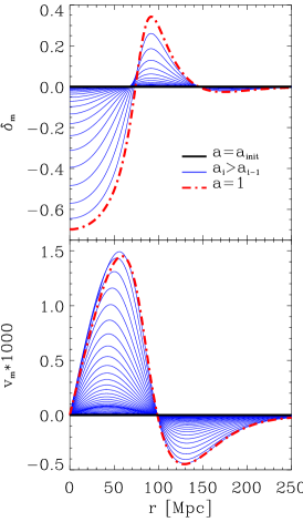
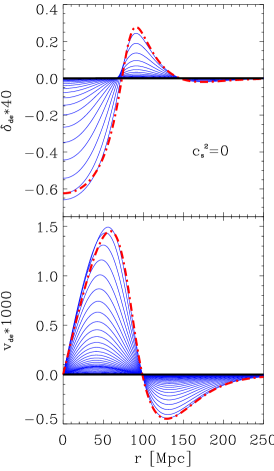
Figure 2: Formation of void with initial profile parameters $\kappa^{-1}=62.8$ Mpc and $\kappa r_{\rm d}=4/3$ in dark matter (left-hand column) and dark energy with $c_{\rm s}^{2}=0$ (central column). In the right-hand column the evolution of absolute values of amplitudes of density (top panel) and velocity (bottom panel) perturbations for void and overdense shell are shown. Other cosmological and dark energy parameters are the same as in Fig. 1. The dotted lines show the evolution of absolute values of amplitudes of density and velocity perturbations for radiation component in the void only.

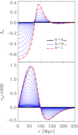
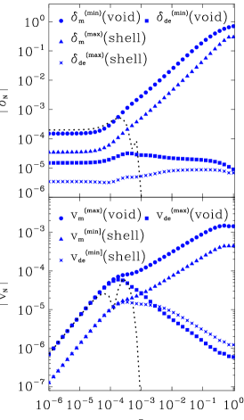
Figure 3: The same as in Fig. 2 for dark energy with $c_{\rm s}^{2}=0.1$.

4 Formation of voids in the cosmological models with dark energy

The results of integration of the system of evolution equations (1)-(7) for initial perturbation, which is shown in the left-hand column of Fig. 1, are shown in Fig. 2 for the model with dark energy parameters $\Omega_{\rm de}=0.7$, $w=-0.9$ and $c_{\rm s}^{2}=0$. The black thick solid lines denote the initial profiles of density and velocity perturbations of matter (left-hand column) and dark energy (central column) at $a_{\rm init}=10^{-6}$, the red thick dash–dotted lines denote the final ones at $a=1$, the blue thin solid ones show for intermediate values of $a$. The figure on the right depicts the evolution of absolute values of amplitudes of perturbations in the central point of spherical void and in the overdense shell. Velocity perturbation (bottom panel) are given for the first maximum (circles and squares, which superimposed) and the first minimum (triangles and fourfold stars, which superimposed). The signs in the right-hand column correspond to the values in the mentioned positions in the corresponding curves in the left-hand and central columns. Dotted lines denote the evolution of the same values for the radiation component. One can see that in this dark energy model the perturbations of matter and dark energy grow monotonically after entering the horizon: the black lines are internal, the red lines are external. We also note that the amplitude of the density perturbation of dark energy is approximately 40 times smaller than the one of matter. The values of velocity perturbations of matter and dark energy in this model of dark energy are the same throughout the evolution of the void. They increase monotonically from $a_{\rm init}$ to $a\approx 0.56$. It is easy to see that the latter value corresponds to the moment of change from the decelerated expansion of the Universe to the accelerated one. The evolution of the absolute values of density and velocity perturbations of matter and dark energy in the overdense shell is similar to the evolution of those in centre.

The similar results of modelling of the void formation in the matter and dark energy with $c_{\rm s}^{2}=0.1$ are shown in Fig. 3. One can see that evolution of matter density and velocity perturbations is practically the same, while for dark energy it has changed drastically. The final profiles of dark energy perturbations (red dash–dotted lines) have very small amplitudes. It means that dark energy in the voids is only slightly perturbed. The right figure explains such behaviour of dark energy during the void formation: the velocity perturbation after the entering into horizon decrease quickly, and density perturbation slightly changes during all stages and in the current epoch $\rho_{\rm de}(1,0)$ does not differ significantly from the background value: $\delta_{\rm de}(1,0)\approx-9\times 10^{-6}$. We see also that the evolution of the absolute values of density and velocity perturbations of dark energy in the overdense shell slightly differ from the evolution of ones in the centre of the void. At the current epoch they are approximately equal small magnitudes.

The perturbations of dark energy with larger values of effective speed of sound after entering the particle horizon is smoothed out even faster. The ratio of densities of dark energy and matter in the centre of the void is

$$\frac{\rho_{\rm de}(1,0)}{\rho_{\rm m}(1,0)}=\frac{1+\delta_{\rm de}(1,0)}{1+\delta_{\rm m}(1,0)}\frac{\Omega_{\rm de}}{\Omega_{\rm m}},$$

and in the case of evolution with considered initial condition this ratio is two to five times larger than on cosmological background.

Table 1: The final parameters of voids (matter density perturbations at the centre $\delta_{\rm c}$, matter density perturbation in the overdense shell $\delta_{\rm sh}$, distance $r_{\rm sh}$ where shell is densest, maximal peculiar velocity of matter $\mathpzc{v}_{\rm m}^{\rm(max)}$, distance $r_{\rm mv}$ where $\mathpzc{v}_{\rm m}=\mathpzc{v}_{\rm m}^{\rm(max)}$, final size of void $r_{\delta=0}^{\rm(final)}$) with different initial parameters $r_{\delta=0}^{\rm(init)}$, $r_{\rm d}$ and $C$. The rest of parameters are the same as in Fig. 3.

$r_{\delta=0}^{\rm(init)}$,	$r_{\rm d}$,	$C\times 10^{4}$	$\delta_{\rm c}$	$\delta_{\rm sh}$	$r_{\rm sh}$,	$\mathpzc{v}_{\rm m}^{\rm(max)}$,	$r_{\rm mv}$,	$\frac{\mathpzc{v}_{\rm m}^{\rm(max)}}{\mathpzc{v}_{\rm H}}$	$r_{\delta=0}^{\rm(final)}$,
(Mpc)	(Mpc)				(Mpc)	(km s-1)	(Mpc)		(Mpc)
31.4	36.3	-1	-0.68	0.33	45.7	202	29.9	0.097	36.9
31.4	25.6	-1	-0.69	0.16	38.6	169	24.6	0.098	29.9
31.4	18.1	-1	-0.73	0.09	31.8	148	20.1	0.11	25.1
62.8	72.5	-1	-0.51	0.14	91.3	237	52.7	0.064	68.5
62.8	51.3	-1	-0.54	0.09	73.8	204	40.4	0.072	57.9
62.8	36.3	-1	-0.59	0.06	59.7	186	33.4	0.080	47.4
62.8	72.5	-2	-0.70	0.34	91.3	428	59.7	0.10	73.8
62.8	51.3	-2	-0.72	0.20	73.8	365	47.4	0.11	61.5
62.8	36.3	-2	-0.77	0.14	59.7	329	40.4	0.12	50.9

The matter density perturbation in the central part of this void at the current epoch is $\delta_{\rm c}\approx-0.7$, the magnitude of density perturbation in the overdense shell is $\delta_{\rm sh}\approx 0.34$, these values are close to the mean ones in the real voids (Mao et al., 2016). The maximum of peculiar velocity of matter which move from centre is $\mathpzc{v}_{\rm m}^{\rm(max)}\approx 1.43\times 10^{-3}c\approx 428$ km s^-1 at $r_{\rm mv}\approx 59.7$ Mpc. The Hubble flow at such distance from the centre is $V_{\rm H}=H_{0}r_{\rm mv}\approx 4179$ km s^-1, so the maximum of peculiar velocity of matter in units of Hubble one at the same distance is $\mathpzc{v}_{\rm m}^{\rm(max)}/V_{\rm H}\approx 0.1$. The distance where the matter density perturbation becomes zero is now $r_{\delta=0}^{\rm(final)}\approx 73.8$ Mpc. Thus, in this model the comoving radius of void has increased approximately in 1.2 times. The same final parameters of voids for different initial $r_{\delta=0}^{\rm(init)}$, $r_{\rm d}$ and $C$ are presented in the Table LABEL:final_void_par. It gives us the possibility to understand how each of parameters of initial profile affects the parameters of final voids. For example, increasing the size of seed perturbation $r_{\delta=0}^{\rm(init)}$ with unchanged other parameters (first and sixth rows) results in increased final size $r_{\delta=0}^{\rm(final)}$ but decreased magnitude of density perturbations in the centre $\delta_{\rm c}$ and in the overdense shell $\delta_{\rm sh}$ as well as the value of maximal peculiar velocity $\mathpzc{v}_{\rm m}^{\rm(max)}$. The decreasing of $r_{\rm d}$ with unchanged other parameters (rows 1-3 rows 4-6, rows 7-9) leads to decreasing of void size, maximal value of peculiar velocity, magnitude of density perturbations in the overdense shell and matter density at the void centre. If $r_{\rm d}<r_{\delta=0}^{\rm(init)}$ then the final void size $r_{\delta=0}^{\rm(final)}$ becomes smaller than initial one (third, sixth and ninth rows). The decreasing of $\kappa$ (increasing of $r_{\delta=0}$) for fixed $\kappa^{2}r_{\rm d}^{2}$ and the same rest parameters leads to the decrease of final amplitude of density perturbation and to the increase of final amplitude of peculiar velocity in the void as well as in the overdensity shell. However, comparing the final values of void parameters in rows 1–4, 2–5 and 3–6 of the Table LABEL:final_void_par shows that they are not simply rescaled, as it might seem by visual comparison of Figs. 2 and 3 of this paper with rigs. 1 and 2 in our paper (Tsizh & Novosyadlyj, 2016). The increasing of initial amplitude $C$ with unchanged other parameters (comparing of values in the rows 4, 5, 6 with corresponding values in the rows 7, 8, 9) leads to increasing the final size of void, the amplitude of density perturbations at the centre and in overdense shell as well as the value of maximal velocity of matter.

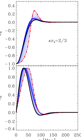
Figure 4: Evolution of normalized profiles of matter density and velocity perturbations with initial parameters $\kappa=(62.8)^{-1}$ Mpc^-1 and $\kappa^{2}r_{\rm d}^{2}=4/3$ (left-hand), 2/3 (central) and 1/3 (right-hand column). Thick black solid lines are normalized initial profiles (Fig. 1), thick red dash–dotted ones are final profiles and blue lines are for intermediate increasing values of $a$. Other parameters are the same as in Fig. 3.

Let us analyse the evolution of matter density profile regardless of their amplitudes. For that, we renormalize each curve in the left-hand columns of Figs 2 and 3 by its amplitude. The results are shown in Fig. 4 for initial perturbations with three different values of $\kappa^{2}r_{\rm d}^{2}=4/3,\,2/3,\,1/3$ and the same other parameters as in previous figures. First of all, we note that the profiles of matter density and velocity perturbations vary with time. They become less steep at the centre and more steep at the edge of void and in the region of overdense shell. One can also see that overdense shell appears in the process of evolution of void even if its amplitude was very small in the initial profile (figure on the right), or absence at all ($\kappa=0$, Gaussian initial profile). The relations between final amplitudes of shell density perturbations have changed essentially: $\delta_{\rm sh}^{(4/3)}:\delta_{\rm sh}^{(2/3)}:\delta_{\rm sh}^{(1/3)}\approx 2.4:1.5:1$ for voids with $r_{\delta=0}^{\rm(init)}=62.8$ Mpc and $C=-2\times 10^{-4}$. In the units of magnitudes of central density perturbations the magnitudes of overdense shells for these profiles now are 0.49, 0.28 and 0.19 against 0.23, 0.055 and 0.006 for initial profiles. They depend also on initial amplitude and scale of the void seeds of the same profile. For example, for voids with $r_{\delta=0}^{\rm(init)}=62.8$ Mpc and $C=-1\times 10^{-4}$ the final magnitudes of overdense shells in the units of magnitudes of central density perturbations are 0.28, 0.16 and 0.10 for three profiles accordingly. For voids with $r_{\delta=0}^{\rm(init)}=31.4$ Mpc and the same $C$ these numbers are 0.49, 0.23 and 0.13, close to the ones for voids with $r_{\delta=0}^{\rm(init)}=62.8$ Mpc and $C=-2\times 10^{-4}$. It explains the similarity of normalized profiles in Fig. 4 and in fig. 3 of Tsizh & Novosyadlyj (2016).

We must to note also that voids with considered sizes and amplitudes (see Table LABEL:final_void_par) do not show tendency to collapse of voids with an overdense shell, which have been discussed in Sheth & van de Weygaert (2004) and Ceccarelli et al. (2013). The void size $r_{\delta=0}$ increases monotonically with $a$ from $a_{\rm init}$ up to $a=1$ in the left-hand panel of Fig. 4, and increases monotonically after formation of overdense shell in the central and right-hand ones. Similar behaviour is demonstrated also by position of the peak density of overdense shells $r_{\rm sh}\equiv r_{max\,\{\delta_{\rm m}\}}$. For the final profiles in the top panels of Fig. 4 they are $r_{\rm sh}=91.3,\,73.8,\,59.7$ Mpc from left to right accordingly. It can be associated with watershed ridgelines in the algorithms of void finding in the galaxies catalogues and snapshots of $N$-body simulations (Platen et al., 2007; Neyrinck et al., 2008; Sutter et al., 2014a). One can consider also the radius of overdense shell as the radius of the sphere on which the peculiar velocity of matter is zero $r_{\mathpzc{v}_{\rm m}=0}$ and change of sign from ‘+’ to ‘–’. For the final profiles in the bottom left-hand and central panels of Fig. 4 they are $r_{\mathpzc{v}_{\rm m}=0}=98.3,\,94.8$ Mpc, respectively. The peculiar velocity shown in the bottom-right panels is positive in all range of $r$. The value of $r_{\mathpzc{v}_{\rm m}=0}$ grows with time too, as it is shown in the figures. So, since these scale parameters are in the frame, which is comoving to cosmological background, the stage of evolution is far from turnaround point, which is begin of the collapse.

Figure 5: The relative perturbations of mass of matter for three profiles with $\kappa^{2}r_{\rm d}^{2}=4/3$ (solid lines), 2/3 (dashed lines) and 1/3 (dotted lines) for initial matter density perturbations profiles (left-hand panel) and for final ones (right-hand panel).

Now consider how the relative perturbation of mass of matter in the sphere of radius $r$, which equals the integrated density contrast,

$$\Delta_{\rm m}(r)=\frac{3}{r^{3}}\int_{0}^{r}\delta_{\rm m}(q)q^{2}dq,$$ (10)

is changed under void formation. In the left-hand panel of Fig. 5, we present the relative perturbations of mass of matter for three initial profiles of matter density perturbations and in the right-hand panel for the final ones. One can see that relative perturbation of mass for density profile with $\kappa^{2}r_{\rm d}^{2}=4/3$ change the sign in the region of overdense shell at the distance $r_{\Delta=0}=98.3$ Mpc and for outer observer it is positive perturbations of mass (overcompensated void or void-in-cloud; (Sheth & van de Weygaert, 2004)). Such voids may exhibit infall velocities of matter in the outer layers of overdense shells and neighbour voids may gravitationally attract. For density profile with $\kappa^{2}r_{\rm d}^{2}=2/3$ the relative perturbation of mass becomes zero inside the shell at the distance $r_{\Delta=0}=94.8$ Mpc and remains so for larger distances from the centre. Note also that $r_{\Delta=0}=r_{\mathpzc{v}_{\rm m}=0}$, which was expected. For density profile with $\kappa^{2}r_{\rm d}^{2}=1/3$ the relative perturbation of mass does not change the sign and remains so for larger distances from the centre and for outer observer it is negative perturbations of mass (undercompensated void). Such neighbour voids may coalesce and form larger non-spherical void. The result of evolution of void is increasing of amplitude of mass perturbation almost 5000 times and redistribution of matter between the marginal part of void and overdense shell (see profiles for peculiar velocity in Figs.2-4). The possibility of collapse of voids with overdense shell is determined by the sign of total mechanical energy of the system, not only by the sign of perturbation of total mass.

5 Universal void profile and its evolution

Let us compare our profiles with universal density profiles for cosmic voids proposed by Hamaus et al. (2014):

$$\delta_{\rm m}(r)=\delta_{\rm c}\left[1-\left(\frac{r}{r_{\rm s}}\right)^{\alpha}\right]/\left[1+\left(\frac{r}{r_{\rm\mathpzc{v}}}\right)^{\beta}\right].$$ (11)

We approximate the final matter density profile matching parameters $r_{\rm s}$, $\alpha$, $r_{\rm\mathpzc{v}}$ and $\beta$ by the Levenberg–Marquardt method (Press et al., 1993). For that, we have used the subroutine mrqmin.f from the Numerical Recipes Library. The value of $\delta_{\rm c}$ we take equal $\delta_{\rm m}(a,0)$ in each specific profile. In the left-hand panel of Fig. 6 we show the matter density perturbation profile for the void model with parameters from the last row of Table LABEL:final_void_par and its approximation by equation (11) with best-fitting parameters $r_{\rm s}=51,457$ Mpc, $\alpha=3.2141$, $r_{\rm\mathpzc{v}}=55.709$ and $\beta=11.31$. These lines are superimposed on one another.

In the right-hand panel of Fig. 6 we show the matter peculiar velocity profile for the same void model. The dotted line presents the peculiar velocity profile which follows from the linear theory of cosmological perturbations $\mathpzc{v}_{\rm lin}(r)\approx-\frac{1}{3}\Omega_{\rm m}^{\gamma}\Delta_{\rm m}(r)H_{0}r$, where $\Delta_{\rm m}(r)$ is relative perturbation of mass (10) and $\gamma\approx 0.55$ (Peebles, 1980). It coincides with velocity profile computed by formula 6 from Hamaus et al. (2014) with parameters presented above for density. In the range of maximum of velocity they differ by factor of $\sim 1.2$, since the later stages of void evolution are not linear. That is why we propose other simple formula for approximation of peculiar velocity profile of matter in the spherical voids:

$$\mathrm{v}_{\rm m}(r)=10^{-3}\left(\frac{r}{r_{\rm lv}}+\frac{r^{3}}{r_{\rm 3v}^{3}}-\frac{r^{5}}{r_{\rm 5v}^{3}}\right)e^{-r^{2}/r_{\rm dv}^{2}}\,\,\,{\rm km\,s^{-1}},$$ (12)

which is the convolution of odd degree polynomial and Gaussian. In the Fig. 6, this approximation with best-fitting parameters $r_{\rm lv}=30.95$ Mpc, $r_{\rm 3v}=28.73$ Mpc, $r_{\rm 5v}=49.05$ Mpc and $r_{\rm dv}=36.33$ Mpc is shown by solid thin blue line. For the $r_{\rm mv}=40.4$ Mpc, we obtain $\mathrm{v}_{\rm m}^{\rm max}\approx 330$ km s^-1. The velocity computed according to the formula of linear theory in this point is $\mathpzc{v}_{\rm lin}^{\rm max}\approx 290$ km s^-1. This approximation formula for peculiar velocity has the property that in the centre part of the void the velocity is proportional to the distance.

Figure 6: Left-hand panel: the final profile of matter density for the model with parameters from the last row of Table LABEL:final_void_par (dash–dotted red line) and its approximation (solid thin blue line) by universal density profile (equation 11). Right-hand panel: the final profile of matter peculiar velocity (dash–dotted red line) and its approximation (solid thin blue line) by convolution of cubic parabola and Gaussian (equation 12). The dotted line is linear velocity $\mathpzc{v}_{\rm lin}$ for density profile from the left-hand panel.

Let us look how parameters $r_{\rm s}$, $\alpha$, $r_{\rm\mathpzc{v}}$ and $\beta$ changed for time of evolution. For that, we approximate the matter density profiles with $\kappa^{2}r_{\rm d}^{2}=4/3,\,\,2/3$ and 1/3 at redshifts $z=10^{6},\,10,\,1,\,0.5$ and 0 matching the parameters of the universal density profile by the Levenberg–Marquardt method for each profile computed in our models of voids. The results are presented in the Fig. 7 by different symbols (cirque, square, triangle) for different initial profiles ($\kappa^{2}r_{\rm d}^{2}=4/3$, 2/3, 1/3 accordingly) and by different colours for different redshifts (black for $z=10^{6}$, dark blue for $z=10$, blue for $z=1$, light blue for $z=0.5$ and red for $z=0$). The evolution of parameters is shown in the left-hand panel of Fig. 7. One can see that scale parameters $r_{\rm s}$ and $r_{\rm\mathpzc{v}}$ as well as power-law parameters $\alpha$ and $\beta$ monotonically increase, which reflect the increase of sizes and amplitude of voids and surrounding overdense shells as well as steepness of their walls.

To compare our profiles of spherical voids with stacked ones from $N$-body simulations we impose these parameters of universal profiles on fig. 2 of Hamaus et al. (2014). In the right-hand panel of Fig. 7 we show the parameters $\delta_{\rm c}$, $\alpha$ and $\beta$ for corresponding $r_{\rm s}/r_{\rm\mathpzc{v}}$. One can see that parameters of profiles of our voids at different redshifts occupy mainly the same regions of parameter space where voids from $N$-body simulations are stacked.

Figure 7: Left-hand panels: the evolution of the best-fitting values of parameters of universal void profile ($r_{\rm s}$, $r_{\rm\mathpzc{v}}$, $\alpha$ and $\beta$) matching the matter density perturbations at different redshifts (from left to right: black at $z=10^{6}$, dark blue at $z=10$, blue at $z=1$, light blue at $z=0.5$ and red at $z=0$) and different initial profile (cirques for $\kappa^{2}r_{\rm d}^{2}=4/3$, squares for $\kappa^{2}r_{\rm d}^{2}=2/3$ and triangles for $\kappa^{2}r_{\rm d}^{2}=1/3$). In the top left-hand panel the open symbols are for $r_{\rm\mathpzc{v}}$, closed for $r_{\rm s}$. Right-hand panels: comparison of the best-fitting values of parameters of universal void profile for our voids with parameters of profiles of voids obtained from $N$-body simulations by Hamaus et al. (2014) (points with error bars and lines). In the top panel the evolution goes top-down and in the middle and bottom ones it goes bottom-top. The initial radius of all voids here is 62.8 Mpc, the initial amplitude is $C=-2\times 10^{-4}$.

We note also that void profiles, obtained here by modelling of their formation from cosmological perturbations with spherical initial profiles, have parameters close to stacked voids from the galaxy catalogues (Sutter et al., 2012; Nadathur & Hotchkiss, 2014; Mao et al., 2016).

6 Sensitivity of void parameters to dark energy ones

We estimated how amplitudes of density and velocity perturbations in the void models are sensitive to the dark energy parameters, especially to $c_{\rm s}^{2}$ and $w$. For that we have computed the evolution of perturbations with the same initial conditions and different $c_{\rm s}^{2}=0,\,0.01,\,0.1,\,1$ and $w=-0.8,\,-0.9,\,-1,\,-1.1,\,-1.2$. The results show that the amplitudes of density perturbations of the void $\delta_{\rm c}$ with parameters in Table LABEL:final_void_par for $c_{\rm s}^{2}=0$ and 1 differ in $\leq 0.2$ per cent, the amplitudes of density perturbations of the overdense shell $\delta_{\rm sh}$ differ in $\leq 0.5$ per cent and the maximal values of matter peculiar velocity $\mathpzc{v}_{\rm m}^{\rm max}$ differ in $\leq 1.6$ per cent. So, the parameters of spherical void models very slightly depend on effective sound speed of dark energy. But the same parameters of spherical void models depend strongly on the value of equation-of-state parameter $w$. Comparing $\delta_{\rm c}$, $\delta_{\rm sh}$ and $\mathpzc{v}_{\rm m}^{\rm max}$ for $w=-0.8$ and –1 we obtain the difference in $\sim 4$ per cent, $\sim 9$ per cent and $\sim 7$ per cent respectively. Comparison of $\delta_{\rm c}$, $\delta_{\rm sh}$ and $\mathpzc{v}_{\rm m}^{\rm max}$ for $w=-1.2$ and -1 gives differences in $\sim 2$ per cent, $\sim 6$ per cent and $\sim 4$ per cent, respectively, but with opposite sign. Therefore, an accurate measurement of matter density and peculiar velocities of galaxies in the voids can be powerful discriminator between quintessence, phantom and $\Lambda$ models of dark energy.

7 Conclusions

The large voids in the spatial distribution of galaxies are formed from the large-scale dips in the Gaussian random field of primordial density perturbations. Such dips with initial radius $r_{\rm s}\sim 30-60$ Mpc (in comoving coordinates) and initial amplitudes $\sim-1\times 10^{-4}$ to $-2\times 10^{-4}$ ($\sim$1–3 rms value in the concordance $\Lambda$CDM model) result into voids with central density perturbation $\sim-0.5$ to $-0.8$ and maximal value of peculiar velocity $\sim$ 150–430 km s^-1 which is directed outward and is reached at the distance $\sim$0.7–0.8$r_{\rm s}$ from the centre of the void. The overdense shell is formed around void by raking of outflowing matter and/or infall outer layers. Its position and amplitude of density depend on the amplitude and type of initial profile, overcompensated or undercompensated. The profile of density perturbations of void evolves in such a way that comoving scale parameters of universal profile (Hamaus et al., 2014) $r_{\rm s}$ and $r_{\rm\mathpzc{v}}$ are increased by $\sim$1.1–1.2 times, the steepness parameters $\alpha$ and $\beta$ are increased by $\sim$2.2–3.0 times.

The density and velocity perturbations of the dark energy evolve similarly to the perturbations of matter at the stage when their scales are much larger than the particle horizon. After they enter the particle horizon their evolution depends on the value of the effective speed of sound $c_{\rm s}$. If $c_{\rm s}=0$, then similarity is conserved with the difference that the amplitude of density perturbation of dark energy is smaller in factor $1+w$. At the later epoch, when the dark energy density dominates, this difference increased yet in $\approx$4–5 times more. If $0<c_{\rm s}\leq 1$, then the amplitude of velocity perturbation of dark energy after entering the horizon decreases rapidly, the amplitude of the density perturbation does not increase or even decreases too. Therefore, in the voids the density of dynamical dark energy is approximately the same as in the cosmological background. The ratio of the densities of dark energy and matter is $1/(1+\delta_{\rm m})$ larger than that in the cosmological background. The more hollow void is the larger this ratio is. Our estimations show, that measurable parameters of large spherical voids with size $\sim 60$ Mpc and typical amplitude of initial perturbation are sensitive to equation-of-state parameters of dark energy $w$ at the level of few per cents and to effective sound speed at the level of 1 per cent. It means that investigation of structure and dynamics of large voids are perspective for testing of models of dark energy and gravity modifications.

References

- Bennett et al. (2013) Bennett C.L. et al., 2013, ApJS, 208, 20
- Biswas et al. (2010) Biswas R., Alizadeh E. & Wandelt B.D., 2010, Phys. Rev. D, 82, 023002
- Bos et al. (2012) Bos E.G.P., van de Weygaert R., Dolag K. & Pettorino, V., 2012, MNRAS, 426, 440
- Cai et al. (2015) Cai Y.-C., Padilla N. & Li B., 2015, MNRAS, 451, 1036
- Ceccarelli et al. (2013) Ceccarelli L., Paz D., Lares M., Padilla N., Lambas D. G., 2013, MNRAS, 434, 1435
- Clampitt et al. (2013) Clampitt J., Cai Y.-C. & Li B., 2013, MNRAS, 431, 749
- Dai (2015) Dai D.-C., 2015, MNRAS, 454, 3590
- Demchenko et al. (2016) Demchenko V., Cai Y.-C., Heymans C., Peacock J. A., 2016, MNRAS, 463, 512
- Falck (2016) Falck B., 2016, Am. Astron. Soc. Meeting Abstr., 227, 223.01
- Gottloeber et al. (2003) Gottloeber S., Lokas E.L., Klypin A. & Hoffman Y., 2003, MNRAS, 344, 715
- Gregory & Thompson (1978) Gregory S.A. & Thompson L.A., 1978, ApJ, 222, 784
- Hamaus et al. (2014) Hamaus N., Sutter P.M. & Wandelt B.D., 2014, Phys. Rev. Lett., 112, 251302
- Hamaus et al. (2015) Hamaus N., Sutter P.M., Lavaux G. & Wandelt B.D., 2015, J. Cosmol. Astropart. Phys., 11, 036
- Hu & Sugiyama (1995) Hu W., Sugiyama N., 1995, ApJ, 444, 489
- Jennings et al. (2013) Jennings E., Li Y. & Hu W., 2013, MNRAS, 434, 2167
- Joeveer et al. (1978) Joeveer M., Einasto J & Tago E. 1978, MNRAS, 185, 357
- Kulinich et al. (2013) Kulinich Yu., Novosyadlyj B. & Apunevych S., 2013, Phys. Rev. D, 88, 103505
- Leveque et al. (1998) Leveque R.J., Mihalas D., Dorfi E.A., Muller E., Computational methods for astrophysical fluid flow, 1998, Springer-Verlag, Berlin
- Lewis et al. (2000) Lewis A., Challinor A. & Lasenby A., 2000, ApJ, 538, 473
- Li et al. (2012) Li B., Zhao G.-B. & Koyama K., 2012, MNRAS, 421, 3481
- Li & Zhao (2009) Li B. & Zhao H., 2009, Phys. Rev. D, 80, 044027
- Mao et al. (2016) Mao Q. et al., 2016, preprint (arXiv:1602.02771)
- Neyrinck et al. (2008) Neyrinck M. C., 2008, MNRAS, 386, 2101
- Nadathur & Hotchkiss (2014) Nadathur S. & Hotchkiss S., 2014, MNRAS, 440, 1248
- Novosyadlyj et al. (2016) Novosyadlyj B., Tsizh M. & Kulinich Yu., 2016, Gen. Relativ. Grav. 48, 3
- Pan et al. (2012) Pan D. C., Vogeley M. S., Hoyle F., Choi Y.-Y., Park C., 2012, MNRAS, 421, 926
- Peebles (1980) Peebles P. J. E., The large scale structure of the Universe. 1980, Princeton Univ. Press, Princeton, NJ
- Planck Collaboration (2015) Planck Collaboration XIII, 2016, AA, 594, A13
- Platen et al. (2007) Platen E., van de Weygaert R. & Jones B. J. T., 2007, MNRAS, 380, 551
- Press et al. (1993) Press W.A., Teukolsky S.A., Vetterling W.T. & Flannery B.P., 1993, Numerical recipes in FORTRAN. The art of Scientific Computing, 2nd edn. Cambridge Univ. Press, Cambridge
- Savitzky & Golay (1964) Savitzky A. & Golay M.J.E., 1964, Anal. Chem., 36, 1627
- Sergijenko & Novosyadlyj (2015) Sergijenko O. & Novosyadlyj B., 2015, Phys. Rev. D 91, 083007
- Sheth & van de Weygaert (2004) Sheth R.K. & van de Weygaert R., 2004, MNRAS 350, 517
- Sutter et al. (2012) Sutter P. M., Lavaux G., Wandelt B.D. & Weinberg D.H., 2012, ApJ, 761, 44
- Sutter et al. (2014a) Sutter P. M., Lavaux G., Wandelt B. D., Weinberg D. H., Warren M. S., 2014a, Mon. Not. R. Astron. Soc., 438, 3177
- Sutter et al. (2014b) Sutter P. M., Lavaux G., Wandelt B.D., Weinberg D.H., Warren M.S., Pisani A., 2014b, MNRAS, 442, 3127
- Sutter et al. (2014c) Sutter P. M., Pisani A., Wandelt B.D., Weinberg D.H., 2014c, MNRAS, 443, 2983
- Sutter et al. (2014d) Sutter P. M., Elahi P., Falck B., Onions J., Hamaus N., Knebe A., Srisawat C., Schneider A., 2014d, MNRAS, 445, 1235
- Tsizh & Novosyadlyj (2016) Tsizh M., Novosyadlyj B., 2016, Adv. Astron. Space Phys., 6, 28
- Woltak et al. (2016) Wojtak R., Powell D., Abel T., 2016, MNRAS, 458, 4431