Abstract

We holographically study supersymmetric deformations of $N=3$ and $N=1$ superconformal field theories (SCFTs) in three dimensions using four-dimensional $N=4$ gauged supergravity coupled to three-vector multiplets with non-semisimple $SO(3)\ltimes(\mathbf{T}^{3},\hat{\mathbf{T}}^{3})$ gauge group. This gauged supergravity can be obtained from a truncation of eleven-dimensional supergravity on a tri-sasakian manifold and admits both $N=1,3$ supersymmetric and stable non-supersymmetric $AdS_{4}$ critical points. We analyze the BPS equations for $SO(3)$ singlet scalars in details and study possible supersymmetric solutions. A number of RG flows to non-conformal field theories and half-supersymmetric domain walls are found, and many of them can be given analytically. Apart from these “flat” domain walls, we also consider $AdS_{3}$-sliced domain wall solutions describing two-dimensional conformal defects with $N=(1,0)$ supersymmetry within the dual $N=1$ field theory while this type of solutions does not exist in the $N=3$ case.

1 Introduction

In recent years, superconformal field theories (SCFTs) in three dimensions have attracted much attention in the context of the AdS/CFT correspondence [1]. Apart from being effective world-volume theories of M2-branes [2, 3], three-dimensional gauge theories and their conformal fixed points have also interesting applications in condensed matter physics [4, 5, 6].
Along this line, four-dimensional gauged supergravities have been a very useful tool in various holographic studies including the holographic Renormalization Group (RG) flows and conformal defects of co-dimension one. The former can be described holographically by domain walls interpolating between two $AdS$ vacua or between an $AdS$ vacuum in one limit and a domain wall in the other limit, see for example [7, 8, 9]. These two classes of solutions correspond respectively to RG flows between conformal fixed points and flows to non-conformal field theories. These solutions are called “flat” or Minkowski-sliced domain walls. The conformal defects on the other hand can be described in the holographic context by AdS-sliced domain walls [10, 11, 12, 13, 14, 15, 16].
A number of holographic RG flows within four-dimensional gauged supergravities have been studied, see for example [17, 18, 19, 20, 21] and [22, 23, 24] for more recent results. Some of these solutions can be uplifted to eleven dimensions resulting in many interesting geometric interpretations such as a polarization of M2-branes into M5-branes in [25]. On the other hand, supersymmetric Janus solutions in four dimensions have been studied recently in the maximal $N=8$, $SO(8)$ gauged supergravity in [26]. Some of these solutions have been uplifted to eleven dimensions via a consistent $S^{7}$ reduction in [25]. In the context of lower supersymmetry, a number of supersymmetric Janus solutions within $N=3$, $SU(2)\times SU(3)$ gauged supergravity have been explored in [27]. This gauged supergravity is expected to describe the lowest Kaluza-Klein modes of a compactification of M-theory on a tri-sasakian manifold $N^{010}$ [28]. The gauge group $SU(2)\times SU(3)$ is an isometry of $N^{010}$, and the two factors are identified with the $N=3$ $SO(3)_{R}$ R-symmetry and $SU(3)$ flavor symmetry in the dual SCFT, respectively.
The complete spectrum of this compactification has been carried out in [29], and the structure of the supermultiplets has been given in [30]. Furthermore, the dual SCFT to this compactification has been proposed in [31]. It has also been discovered in [31] and further investigated in [32] that all compactifications of M-theory giving rise to $N=3$ supersymmetric $AdS_{4}$ backgrounds contain a universal massive spin-$\frac{3}{2}$ multiplet. All components of this multiplet arise only from constant harmonics. The truncation keeping only the lowest Kaluza-Klein modes and this massive multiplet is accordingly expected to be consistent. The resulting theory is expected to be $N=4$ gauged supergravity with $N=4$ supersymmetry broken to $N=3$ at the vacuum. The dual composite operators to this long, massive, gravitino multiplet have also been proposed in [31, 32].
Up to now, only the complete truncation of eleven-dimensional supergravity on a generic tri-sasakian manifold has been carried out in [33] in which all the fields which are singlet under the flavor $SU(3)$ symmetry have been kept. The enhancement by the Betti vector multiplet, which is also an $SU(3)$ singlet, in the compactification on $N^{010}$ has also been pointed out. This is due to a non-trivial cohomology of degree two in $N^{010}$ giving rise to an additional massless vector multiplet.
This tri-sasakian truncation results in $N=4$ gauged supergravity coupled to three vector multiplets. The theory admits two supersymmetric $AdS_{4}$ solutions with unbroken $SO(3)_{R}$ R-symmetry and $N=3,1$ supersymmetries. These solutions correspond to compactifications on $N^{010}$ and its squashed version, respectively. A possible candidate for the $N=3$ SCFT dual to the $N=3$ solution is given in [31], but there is a puzzle with this SCFT regarding to the baryonic spectrum, see a discussion in [34] and [35]. For the $N=1$ case, the situation is less clear. In particular, the $N=1$ SCFT dual to the squashed $N=1$, $AdS_{4}\times N^{010}$ solution has not previously appeared although the $N=1$ SCFT dual to the squashed $S^{7}$ compactification has been given in [36]. In this paper, we will analyze the BPS equations for $SO(3)_{R}$ invariant scalar fields and investigate possible deformations of the dual $N=3$ and $N=1$ SCFTs within the framework of four-dimensional gauged supergravity.
We will mainly consider supersymmetric deformations in the forms of RG flows to non-conformal field theories and two-dimensional defects described by Janus solutions. Regarding to the $N^{010}$ compactification, a number of holographic RG flows and Janus solutions within the framework of $N=3$ gauged supergravity have already been studied in [37] and [27], but these solutions currently cannot be uplifted to eleven dimensions due to the lack of the complete consistent truncation keeping all lowest Kaluza-Klein modes including the $SU(3)$ non-singlet ones.
The paper is organized as follow. In section 2, we review $N=4$ gauged supergravity coupled to three vector multiplets and the tri-sasakian truncation of eleven-dimensional supergravity to this $N=4$ gauged supergravity. The analysis of BPS equations for $SO(3)_{R}$ singlet scalars will also be carried out. These are relevant for finding supersymmetric RG flow and Janus solutions in sections 3 and 4. We will also explicitly give the uplift of some solutions to eleven dimensions and finally give some conclusions and comments on the results in section 5. In the two appendices, we give an explicit form of the relevant field equations and some of the complicated BPS equations.

2 $N=4$ gauged supergravity and tri-sasakian truncation of eleven-dimensional supergravity

In this section, we briefly review $N=4$ gauged supergravity in the embedding tensor formalism to set up the framework for finding supersymmetric solutions. Further details on the construction can be found in [38] on which this review is mainly based. We will also give basic information and relevant formulae of the tri-sasakian truncation of eleven-dimensional supergravity to $N=4$ gauged supergravity with $SO(3)\ltimes(\mathbf{T}^{3},\hat{\mathbf{T}}^{3})$ gauge group. This is the strategy we will follow in order to uplift four-dimensional solutions to eleven dimensions.

2.1 $N=4$ gauged supergravity coupled to three vector multiplets

We now consider the half-maximal $N=4$ supergravity in four dimensions. The supergravity multiplet consists of the graviton $e^{\hat{\mu}}_{\mu}$, four gravitini $\psi^{i}_{\mu}$, six vectors $A_{\mu}^{m}$, four spin-$\frac{1}{2}$ fields $\chi^{i}$ and one complex scalar $\tau$. The complex scalar, or equivalently two real scalars, can be parametrized by the $SL(2,\mathbb{R})/SO(2)$ coset.
In this half-maximal supersymmetry, the supergravity multiplet can couple to an arbitrary number $n$ of vector multiplets although we will later set $n=3$. Each multiplet contains a vector field $A_{\mu}$, four gaugini $\lambda^{i}$ and six scalars $\phi^{m}$. The scalar fields can be parametrized by the $SO(6,n)/SO(6)\times SO(n)$ coset. Before moving to possible gaugings of this matter-coupled supergravity, we will first give some details on various indices used throughout this paper.
Space-time and tangent space indices are denoted respectively by $\mu,\nu,\ldots=0,1,2,3$ and $\hat{\mu},\hat{\nu},\ldots=0,1,2,3$. The $SO(6)\sim SU(4)$ R-symmetry indices will be described by $m,n=1,\ldots,6$ for the $SO(6)$ vector representation and $i,j=1,2,3,4$ for the $SO(6)$ spinor or $SU(4)$ fundamental representations. The $n$ vector multiplets will be labeled by indices $a,b=1,\ldots,n$. Therefore, all the fields in the vector multiplets will carry an additional index in the form of $(A^{a}_{\mu},\lambda^{ia},\phi^{ma})$. All fermionic fields and the supersymmetry parameters transform in the fundamental representation of $SU(4)_{R}\sim SO(6)_{R}$ R-symmetry and are subject to the chirality projections

$$\gamma_{5}\psi^{i}_{\mu}=\psi^{i}_{\mu},\qquad\gamma_{5}\chi^{i}=-\chi^{i},\qquad\gamma_{5}\lambda^{i}=\lambda^{i}\,.$$ (1)

Similarly, for the corresponding fields transforming in the anti-fundamental representation of $SU(4)_{R}$, we have

$$\gamma_{5}\psi_{\mu i}=-\psi_{\mu i},\qquad\gamma_{5}\chi_{i}=\chi_{i},\qquad\gamma_{5}\lambda_{i}=-\lambda_{i}\,.$$ (2)

Gaugings of the matter-coupled $N=4$ supergravity can be efficiently described by using the embedding tensor $\Theta$. This constant tensor encodes the information about the embedding of any gauge group $G_{0}$ in the global or duality symmetry $SL(2,\mathbb{R})\times SO(6,n)$ in a covariant way. It has been shown in [38] that there are two components of the embedding tensor $\xi^{\alpha M}$ and $f_{\alpha MNP}$ with $\alpha=(+,-)$ and $M,N=(m,a)=1,\ldots,n+6$ denoting fundamental representations of $SL(2,\mathbb{R})$ and $SO(6,n)$, respectively. The electric vector fields $A^{+M}=(A^{m}_{\mu},A^{a}_{\mu})$, appearing in the ungauged Lagrangian, and their magnetic dual $A^{-M}$ form a doublet under $SL(2,\mathbb{R})$ denoted by $A^{\alpha M}$.
In general, a subgroup of both $SL(2,\mathbb{R})$ and $SO(6,n)$ can be gauged, and the magnetic vector fields can also participate in the gauging. In particular, it has been shown in [39], see also [40], that purely electric gaugings do not admit $AdS_{4}$ vacua. In this paper, we will only consider gaugings involving both electric and magnetic vector fields in order to obtain $AdS_{4}$ vacua relevant for applications in the AdS/CFT correspondence.
The full covariant derivative can be written as

$$D_{\mu}=\nabla_{\mu}-gA_{\mu}^{\alpha M}\Theta_{\alpha M}^{\phantom{\alpha M}NP}t_{NP}+gA_{\mu}^{M(\alpha}\epsilon^{\beta)\gamma}\xi_{\gamma M}t_{\alpha\beta}$$ (3)

where $\nabla_{\mu}$ is the usual space-time covariant derivative. $t_{MN}$ and $t_{\alpha\beta}$ are $SO(6,n)$ and $SL(2,\mathbb{R})$ generators which can be chosen as

$$(t_{MN})_{P}^{\phantom{P}Q}=2\delta^{Q}_{[M}\eta_{N]P},\qquad(t_{\alpha\beta})_{\gamma}^{\phantom{\gamma}\delta}=2\delta^{\delta}_{(\alpha}\epsilon_{\beta)\gamma}$$ (4)

with $\epsilon^{\alpha\beta}=-\epsilon^{\beta\alpha}$ and $\epsilon^{+-}=1$. $\eta_{MN}=\textrm{diag}(-1,-1,-1,-1,-1,-1,1,\ldots,1)$ is the $SO(6,n)$ invariant tensor, and $g$ is the gauge coupling constant that can be absorbed in the embedding tensor $\Theta$. The embedding tensor appearing in the above equation can be written in terms of $\xi^{\alpha M}$ and $f_{\alpha MNP}$ as

$$\theta_{\alpha MNP}=f_{\alpha MNP}-\xi_{\alpha[N}\eta_{P]M}\,.$$ (5)

In the following discussions, we will only consider solutions with only the metric and scalars non-vanishing. Therefore, we will set all of the vector fields to zero from now on.
We now consider explicit parametrization of the scalar coset manifold $SL(2,\mathbb{R})/SO(2)\times SO(6,n)/SO(6)\times SO(n)$. The first factor can be described by a coset representative

$$\mathcal{V}_{\alpha}=\frac{1}{\sqrt{\textrm{Im}\tau}}\left(\begin{array}[]{c}\tau\\ 1\\ \end{array}\right)$$ (6)

or equivalently by a symmetric matrix

$$M_{\alpha\beta}=\textrm{Re}(\mathcal{V}_{\alpha}\mathcal{V}^{*}_{\beta})=\frac{1}{\textrm{Im}\tau}\left(\begin{array}[]{cc}|\tau|^{2}&\textrm{Re}\tau\\ \textrm{Re}\tau&1\\ \end{array}\right).$$ (7)

Note that $\textrm{Im}(\mathcal{V}_{\alpha}\mathcal{V}^{*}_{\beta})=\epsilon_{\alpha\beta}$. The complex scalar $\tau$ can in turn be written in terms of the dilaton $\phi$ and the axion $\chi$ as

$$\tau=\chi+ie^{\phi}\,.$$ (8)

For the $SO(6,n)/SO(6)\times SO(n)$ factor, we introduce the coset representative $\mathcal{V}_{M}^{\phantom{M}A}$ transforming by a left and right multiplication under $SO(6,n)$ and $SO(6)\times SO(n)$, respectively. We will split the $SO(6)\times SO(n)$ index $A=(m,a)$ and write the coset representative as $\mathcal{V}_{M}^{\phantom{M}A}=(\mathcal{V}_{M}^{\phantom{M}m},\mathcal{V}_{M}^{\phantom{M}a})$. Being an element of $SO(6,n)$, the matrix $\mathcal{V}_{M}^{\phantom{M}A}$ satisfies the relation

$$\eta_{MN}=-\mathcal{V}_{M}^{\phantom{M}m}\mathcal{V}_{N}^{\phantom{M}m}+\mathcal{V}_{M}^{\phantom{M}a}\mathcal{V}_{N}^{\phantom{M}a}\,.$$ (9)

As in the $SL(2,\mathbb{R})/SO(2)$ factor, we can parametrize the $SO(6,n)/SO(6)\times SO(n)$ coset in term of a symmetric matrix

$$M_{MN}=\mathcal{V}_{M}^{\phantom{M}m}\mathcal{V}_{N}^{\phantom{M}m}+\mathcal{V}_{M}^{\phantom{M}a}\mathcal{V}_{N}^{\phantom{M}a}\,.$$ (10)

We are now in a position to give the bosonic Lagrangian with the vector fields and auxilary two-form fields vanising

$$e^{-1}\mathcal{L}=\frac{1}{2}R+\frac{1}{16}\partial_{\mu}M_{MN}\partial^{\mu}M^{MN}-\frac{1}{4(\textrm{Im}\tau)^{2}}\partial_{\mu}\tau\partial^{\mu}\tau^{*}-V$$ (11)

where $e$ is the vielbein determinant. The scalar potential is given by

$$V = \frac{g^{2}}{16}\left[f_{\alpha MNP}f_{\beta QRS}M^{\alpha\beta}\left[\frac{1}{3}M^{MQ}M^{NR}M^{PS}+\left(\frac{2}{3}\eta^{MQ}-M^{MQ}\right)\eta^{NR}\eta^{PS}\right]\right.$$ (12)

$$\left.-\frac{4}{9}f_{\alpha MNP}f_{\beta QRS}\epsilon^{\alpha\beta}M^{MNPQRS}+3\xi^{M}_{\alpha}\xi^{N}_{\beta}M^{\alpha\beta}M_{MN}\right]$$

where $M^{MN}$ is the inverse of $M_{MN}$, and $M^{MNPQRS}$ is defined by

$$M_{MNPQRS}=\epsilon_{mnpqrs}\mathcal{V}_{M}^{\phantom{M}m}\mathcal{V}_{N}^{\phantom{M}n}\mathcal{V}_{P}^{\phantom{M}p}\mathcal{V}_{Q}^{\phantom{M}q}\mathcal{V}_{R}^{\phantom{M}r}\mathcal{V}_{S}^{\phantom{M}s}$$ (13)

with indices raised by $\eta^{MN}$.
The gauge group we will consider here is a non-semisimple group $SO(3)\ltimes(\mathbf{T}^{3},\hat{\mathbf{T}}^{3})\subset SO(6,3)$ described by the non-vanishing component $f_{\alpha MNP}$ of the embedding tensor. We will then set $\xi^{\alpha M}=0$ in the following discussion. The embedding of this $SO(3)\ltimes(\mathbf{T}^{3},\hat{\mathbf{T}}^{3})$ gauge group is described by the following components of the embedding tensor

$$f_{+IJ,K+6} = -f_{+I+3,J+6,K+6}=-2\sqrt{2}\epsilon_{IJK},\qquad I,J,K=1,2,3,$$

$$f_{+I+6,J+6,K+6} = 6\sqrt{2}k\epsilon_{IJK},\qquad f_{-I,J+6,K+6}=-4\epsilon_{IJK}\,.$$ (14)

The constant $k$ is related to the four-form flux along the four-dimensional space-time, see equation (30) below. This gauge group arises from a truncation of eleven-dimensional supergravity on a tri-sasakain manifold [33]. It should be noted that both electric and magnetic components participate in the gauging, $f_{\pm MNP}\neq 0$, since purely electric gaugings do not lead to $AdS_{4}$ vacua as mentioned above.
We should also remark that the identification of this gauge group and other computations in [33] have been done in the off-diagonal $\eta_{MN}$

$$\eta_{MN}=\left(\begin{array}[]{ccc}-\mathbf{I}_{3}&\mathbf{0}_{3}&\mathbf{0}_{3}\\ \mathbf{0}_{3}&\mathbf{0}_{3}&\mathbf{I}_{3}\\ \mathbf{0}_{3}&\mathbf{I}_{3}&\mathbf{0}_{3}\\ \end{array}\right)$$ (15)

where $\mathbf{0}_{3}$ and $\mathbf{I}_{3}$ denote $3\times 3$ zero and identity matrices, respectively. Accordingly, in computing $M_{MNPQRS}$ in (13) and some parts of the supersymmetry transformations given below, $\mathcal{V}_{M}^{\phantom{M}m}$ and $\mathcal{V}_{M}^{\phantom{M}a}$ must be projected to the negative and positive eigenvalue subspaces of $\eta_{MN}$, respectively.
By transforming to a purely electric frame, the gauge algebra will be more transparent. We will not explicitly give this transformation here since we will mainly work in the above electric-magnetic frame. However, for completeness, we will discuss the structure of the gauge algebra here, see [33] for more details. The $SO(3)$ part is the diagonal subgroup of $SO(3)\times SO(3)\times SO(3)\subset SO(6)\times SO(3)\subset SO(6,3)$. The six generators of $\mathbf{T}^{3}$ and $\hat{\mathbf{T}}^{3}$ transform as $\mathbf{3}+\mathbf{3}$ under $SO(3)$. $\mathbf{T}^{3}$ generators commute with each other while $\hat{\mathbf{T}}^{3}$ generators close on to $\mathbf{T}^{3}$ generators.
We now turn to another important ingredient of the $N=4$ gauged supergravity namely the supersymmetry transformations of fermionic fields. These are given by

$$\delta\psi^{i}_{\mu} = 2D_{\mu}\epsilon^{i}-\frac{2}{3}gA^{ij}_{1}\gamma_{\mu}\epsilon_{j},$$ (16)

$$\delta\chi^{i} = i\epsilon^{\alpha\beta}\mathcal{V}_{\alpha}D_{\mu}\mathcal{V}_{\beta}\gamma^{\mu}\epsilon^{i}-\frac{4}{3}igA_{2}^{ij}\epsilon_{j},$$ (17)

$$\delta\lambda^{i}_{a} = 2i\mathcal{V}_{a}^{\phantom{a}M}D_{\mu}\mathcal{V}_{M}^{\phantom{M}ij}\gamma^{\mu}\epsilon_{j}+2igA_{2aj}^{\phantom{2aj}i}\epsilon^{j}\,.$$ (18)

The fermion shift matrices are defined by

$$A_{1}^{ij} = \epsilon^{\alpha\beta}(\mathcal{V}_{\alpha})^{*}\mathcal{V}_{kl}^{\phantom{kl}M}\mathcal{V}_{N}^{\phantom{N}ik}\mathcal{V}_{P}^{\phantom{P}jl}f_{\beta M}^{\phantom{\beta M}NP},$$

$$A_{2}^{ij} = \epsilon^{\alpha\beta}\mathcal{V}_{\alpha}\mathcal{V}_{kl}^{\phantom{kl}M}\mathcal{V}_{N}^{\phantom{N}ik}\mathcal{V}_{P}^{\phantom{P}jl}f_{\beta M}^{\phantom{\beta M}NP},$$

$$A_{2ai}^{\phantom{2ai}j} = \epsilon^{\alpha\beta}\mathcal{V}_{\alpha}\mathcal{V}^{M}_{\phantom{M}a}\mathcal{V}^{N}_{\phantom{N}ik}\mathcal{V}_{P}^{\phantom{P}jk}f_{\beta MN}^{\phantom{\beta MN}P}$$ (19)

where $\mathcal{V}_{M}^{\phantom{M}ij}$ is defined in terms of the ’t Hooft symbols $G^{ij}_{m}$ and $\mathcal{V}_{M}^{\phantom{M}m}$ as

$$\mathcal{V}_{M}^{\phantom{M}ij}=\frac{1}{2}\mathcal{V}_{M}^{\phantom{M}m}G^{ij}_{m}$$ (20)

an similarly for its inverse

$$\mathcal{V}^{M}_{\phantom{M}ij}=-\frac{1}{2}\mathcal{V}_{M}^{\phantom{M}m}(G^{ij}_{m})^{*}\,.$$ (21)

$G^{ij}_{m}$ satisfy the relations

$$G_{mij}=(G^{ij}_{m})^{*}=\frac{1}{2}\epsilon_{ijkl}G^{kl}_{m}\,.$$ (22)

The explicit form of these matrices can be found for example in [39]. Note that we use the convention about the (anti) self-duality of $G_{mij}$ opposite to that of [39]. It should also be noted that the scalar potential can be written in terms of $A_{1}$ and $A_{2}$ tensors as

$$V=-\frac{1}{3}A^{ij}_{1}A_{1ij}+\frac{1}{9}A^{ij}_{2}A_{2ij}+\frac{1}{2}A_{2ai}^{\phantom{2ai}j}A_{2a\phantom{i}j}^{\phantom{2a}i}\,.$$ (23)

2.2 $N=4$ gauged supergravity from eleven dimensions

Four-dimensional $N=4$ gauged supergravity coupled to three vector multiplets with $SO(3)\ltimes(\mathbf{T}^{3},\hat{\mathbf{T}}^{3})$ gauge group has been obtained from a truncation of eleven-dimensional supergravity on a generic tri-sasakian manifold in [33]. In this section, we review relevant formulae involving the reduction ansatz which will be useful for uplifting four-dimensional solutions in the next sections. In particular, we will set all of the vector fields to zero as well as the auxiliary two-form and magnetic vector fields.
The eleven-dimensional metric can be written as

$$ds^{2}_{11}=e^{2\varphi}ds^{2}_{4}+e^{2U}ds^{2}(B_{\textrm{QK}})+g_{IJ}\eta^{I}\eta^{J}\,.$$ (24)

The three-dimensional internal metric $g_{IJ}$ can be written in terms of the vielbein as

$$g=Q^{T}Q\,.$$ (25)

For convenience, as in [33], we will parametrize the matrix $Q$ in term of a product of a diagonal matrix $V$ and an $SO(3)$ matrix $O$ as

$$Q=VO,\qquad V=\textrm{diag}(e^{V_{1}},e^{V_{2}},e^{V_{3}})\,.$$ (26)

The scalar $\varphi$ is chosen in such a way that the four-dimensional Einstein-Hilbert term is obtained

$$\varphi=-\frac{1}{2}(4U+V_{1}+V_{2}+V_{3}).$$ (27)

Finally, $B_{\textrm{QK}}$ denotes a four-dimensional quaternionic Kahler manifold.
The three-form field and its four-form field strength are given respectively by

$$C_{3}=c_{3}+c_{IJ}\eta^{I}\wedge J^{I}+\frac{1}{6}\chi\epsilon_{IJK}\eta^{I}\wedge\eta^{J}\wedge\eta^{K}$$ (28)

and

$$G_{4} = H_{4}+4\textrm{Tr}c\,\textrm{vol}(\textrm{QK})+\frac{1}{6}\epsilon_{IJK}d\chi\wedge\eta^{I}\eta^{J}\eta^{K}+dc_{IJ}\wedge\eta^{I}\wedge J^{J}$$ (29)

$$\epsilon_{IJL}\left[(\chi+\textrm{Tr}c)\delta_{LK}-2c_{(LK)}\right]\eta^{I}\wedge\eta^{J}\wedge J^{K}$$

where $H_{4}=dc_{3}$, $c_{IJ}$ is a $3\times 3$ matrix and $\textrm{Tr}c=\delta^{IJ}c_{IJ}$. In the present case, the $H_{4}$ will be given by

$$H_{4}=-6ke^{4\varphi-V_{1}-V_{2}-V_{3}-4U}\textrm{vol}_{4}$$ (30)

where $\textrm{vol}_{4}$ is the volume form of the four-dimensional metric $ds^{2}_{4}$. The volume form of $B_{\textrm{QK}}$, $\textrm{vol}(\textrm{QK})$, can be written in terms of the two-forms $J^{I}$ as

$$\textrm{vol}(\textrm{QK})=\frac{1}{6}J^{I}\wedge J^{I}\,.$$ (31)

For the $N^{010}$ tri-sasakian manifold, we can take a simple description in term of a coset manifold $SU(3)/U(1)$. This is enough for our propose although the full $SU(3)\times SU(2)$ isometry is not manifest, see [41] for another description. Using the standard Gell-Mann matrices, we can choose the $SU(3)$ geneartors to be $-\frac{i}{2}\lambda_{\alpha}$, $\alpha=1,\ldots,8$. The coset and $U(1)$ generators can be chosen to be

$$K_{i}=-\frac{i}{2}(\lambda_{1},\lambda_{2},\lambda_{3},\lambda_{4},\lambda_{5},\lambda_{6},\lambda_{7}),\qquad H=-\frac{i\sqrt{3}}{2}\lambda_{8}\,.$$ (32)

The vielbein on $N^{010}$ can eventually be obtained from the decomposition of the Maurer-Cartan one-form

$$L^{-1}dL=e^{i}K_{i}+\omega H$$ (33)

where $L$ is the coset representative for $SU(3)/U(1)$. $\omega$ is the corresponding $U(1)$ connection.
Following [33], we will use the tri-sasakian structures of the form

$$\eta^{I} = \frac{1}{2}(e^{1},e^{2},e^{3}),$$

$$J^{I} = \frac{1}{8}(e^{4}\wedge e^{5}-e^{3}\wedge e^{6},-e^{3}\wedge e^{5}-e^{4}\wedge e^{6},e^{5}\wedge e^{6}-e^{3}\wedge e^{4}).$$ (34)

From these, we find the metric on $B_{\textrm{QK}}$ to be

$$ds^{2}(B_{\textrm{QK}})=\frac{1}{256}\left[(e^{3})^{2}+(e^{4})^{2}+(e^{5})^{2}+(e^{6})^{2}\right]$$ (35)

with the volume form given by

$$\textrm{vol}(\textrm{QK})=\frac{1}{6}J^{I}\wedge J^{I}=-\frac{1}{64}e^{3}\wedge e^{4}\wedge e^{5}\wedge e^{6}\,.$$ (36)

In the remaining parts of this paper, we will not need the explicit form of $ds^{2}(B_{\textrm{QK}})$ and $\eta^{I}$’s since we will not consider the deformations of these metrics. Therefore, we will leave these as generic expressions.

2.3 BPS equations for $SO(3)$ invariant scalars

We now give an explicit parametrization of the $SL(2,\mathbb{R})/SO(2)\times SO(6,3)/SO(6)\times SO(3)$ coset and relevant information for setting up the BPS equations corresponding to $SO(3)$ singlet scalars.
Since we will study both RG flows and Janus solutions, and the former can formally be obtained as a limit of the latter, we will first construct the BPS equations for finding supersymmetric Janus solutions and take an appropriate limit to find the BPS equations for RG flow solutions. The metric ansatz takes the form of an $AdS_{3}$-sliced domain wall

$$ds^{2}=e^{2A(r)}\left(e^{\frac{2\xi}{\ell}}dx^{2}_{1,1}+d\xi^{2}\right)+dr^{2}\,.$$ (37)

As can be clearly seen, this metric becomes a flat domain wall used in the study of holographic RG flows in the limit $\ell\rightarrow\infty$. The vielbein components can be chosen to be

$$e^{\hat{\mu}}=e^{A+\frac{\xi}{\ell}}dx^{\mu},\qquad e^{\hat{\xi}}=e^{A}d\xi,\qquad e^{\hat{r}}=dr\,.$$ (38)

The non-vanishing spin connections of this metric are then given by

$$\omega^{\hat{\xi}}_{\phantom{\hat{\xi}}\hat{r}}=A^{\prime}e^{\hat{\xi}},\qquad\omega^{\hat{\mu}}_{\phantom{\hat{\xi}}\hat{\xi}}=\frac{1}{\ell}e^{-A}e^{\hat{\mu}},\qquad\omega^{\hat{\mu}}_{\phantom{\hat{\xi}}\hat{r}}=A^{\prime}e^{\hat{\mu}}$$ (39)

where ^′ denotes the $r$-derivative. For the moment, indices $\mu,\nu$ will take values $0,1$, and hatted indices are the tangent space indices.
In this paper, we are only interested in $SO(3)$ singlet scalars. These scalar fields depend only on the radial coordinate $r$. There are four $SO(3)$ singlets corresponding to two scalars from $SL(2,\mathbb{R})/SO(2)$ and another two from $SO(6,3)/SO(6)\times SO(3)$ according to the branching of $SO(6,3)\rightarrow SO(3)\times SO(3)\times SO(3)\rightarrow SO(3)_{\textrm{diag}}$

$$(\mathbf{6},\mathbf{3})\rightarrow(\mathbf{3},\mathbf{1},\mathbf{3})+(\mathbf{1},\mathbf{3},\mathbf{3})\rightarrow 2\times(\mathbf{1}+\mathbf{3}+\mathbf{5}).$$ (40)

Following [33], we parametrize the $SO(6,3)/SO(6)\times SO(3)$ coset representative by

$$\mathcal{V}=\textrm{exp}\left(\begin{array}[]{ccc}\mathbf{0}_{3}&\sqrt{2}Z\mathbf{I}_{3}&\mathbf{0}_{3}\\ \mathbf{0}_{3}&\mathbf{0}_{3}&\mathbf{0}_{3}\\ \sqrt{2}Z\mathbf{I}_{3}&\mathbf{0}_{3}&\mathbf{0}_{3}\\ \end{array}\right)\times\left(\begin{array}[]{ccc}\mathbf{I}_{3}&\mathbf{0}_{3}&\mathbf{0}_{3}\\ \mathbf{0}_{3}&e^{-2U-V_{1}}\mathbf{I}_{3}&\mathbf{0}_{3}\\ \mathbf{0}_{3}&\mathbf{0}_{3}&e^{2U+V_{1}}\mathbf{I}_{3}\\ \end{array}\right).$$ (41)

Note that $SO(3)$ invariance requires $c_{IJ}$ to be proportional to the identity, $c_{IJ}=\sqrt{2}Z\delta_{IJ}$, and $V_{1}=V_{2}=V_{3}$.
The $SL(2,\mathbb{R})/SO(2)$ scalars are given by

$$\tau=\chi+ie^{3V_{1}}\,.$$ (42)

For convenience, we will define another scalar

$$U_{1}=2U+V_{1}\,.$$ (43)

This also gives a diagonal scalar kinetic term

$$\frac{1}{16}\partial_{\mu}M_{MN}\partial^{\mu}M^{MN}-\frac{1}{4(\textrm{Im}\tau)^{2}}\partial_{\mu}\tau\partial^{\mu}\tau^{*}=-\frac{3}{2}{U_{1}^{\prime}}^{2}-\frac{9}{4}{V_{1}^{\prime}}^{2}-\frac{1}{4}e^{-6V_{1}}{\chi^{\prime}}^{2}-\frac{3}{2}e^{-2U_{1}}{Z^{\prime}}^{2}\,.$$ (44)

In order to setup the BPS equations corresponding to $\delta\chi^{i}=0$ and $\delta\lambda^{i}_{a}=0$, a projector involving $\gamma_{r}$ is needed. Since the procedure is essentially the same as in [26] and [27], we will only repeat the relevant formulae. Following [26], we will use Majorana representation in which all gamma matrices $\gamma_{\mu}$ are real, and $\gamma_{5}=i\gamma_{\hat{0}}\gamma_{\hat{1}}\gamma_{\hat{\xi}}\gamma_{\hat{r}}$ is purely imaginary. In the chiral notation, we have, for example,

$$\epsilon^{i}=\frac{1}{2}(1+\gamma_{5})\epsilon^{i}_{M},\qquad\epsilon_{i}=\frac{1}{2}(1-\gamma_{5})\epsilon^{i}_{M}$$ (45)

where $\epsilon_{M}$ is a four-component Majorana spinor. From these, it follows that $\epsilon_{i}=(\epsilon^{i})^{*}$.
Accordingly, the $\gamma_{r}$-projector can be written as

$$\gamma^{\hat{r}}\epsilon^{i}=e^{i\Lambda}\epsilon_{i}$$ (46)

or equivalently

$$\gamma^{\hat{r}}\epsilon_{i}=e^{-i\Lambda}\epsilon^{i}\,.$$ (47)

The analysis of $\delta\psi^{i}_{\mu}=0$ equations leads to the following $\gamma_{\hat{\xi}}$ projection

$$\gamma_{\hat{\xi}}\epsilon_{i}=i\kappa e^{i\Lambda}\epsilon^{i}$$ (48)

see [26] for more detail. The constant $\kappa$ satisfying $\kappa^{2}=1$ determines the chirality of the unbroken supercharges on the two-dimensional defect. Up to a phase, the full Killing spinor can be written as

$$\epsilon^{i}=e^{\frac{A}{2}+\frac{\xi}{2\ell}+i\frac{\Lambda}{2}}\varepsilon^{(0)i}$$ (49)

with the constant spinors $\varepsilon^{(0)i}$ satisfying

$$\gamma_{\hat{r}}\varepsilon^{(0)i}=\varepsilon^{(0)}_{i}\qquad\textrm{and}\qquad\gamma_{\hat{\xi}}\varepsilon^{(0)}_{i}=i\kappa\varepsilon^{(0)i}\,.$$ (50)

The integrabitity conditions of $\delta\psi^{i}_{\hat{0},\hat{1}}=0$ equations give

$$A^{\prime 2}+\frac{1}{\ell^{2}}e^{-2A}=|\mathcal{W}|^{2}$$ (51)

where $\mathcal{W}$ is the “superpotential” given by the eigenvalue $\alpha$ of the $A_{1}^{ij}$ tensor corresponding to the unbroken supersymmetry

$$\mathcal{W}=\frac{2}{3}\alpha\,.$$ (52)

The cosmological constant at $AdS_{4}$ critical points is given in term of $\alpha$ by the relation $V_{0}=-\frac{4}{3}\alpha^{2}$.
Finally, we note the expression for the phase $e^{i\Lambda}$ in terms of $\mathcal{W}$

$$e^{i\Lambda} = \frac{A^{\prime}}{W}+\frac{i\kappa}{\ell}\frac{e^{-A}}{W}\,.$$ (53)

$$\textrm{and}\qquad e^{i\Lambda} = \frac{\mathcal{W}}{A^{\prime}+\frac{i\kappa}{\ell}e^{-A}}\,.$$ (54)

for real and complex $\mathcal{W}$, respectively. These relations can be obtained by considering the gravitino variations in each case, see [27] for more detail.
For the RG flows, the corresponding BPS equations can be found by formally taking the limit $\ell\rightarrow\infty$. We simply find

$$A^{\prime}=\pm W\qquad\textrm{and}\qquad e^{i\Lambda}=\frac{\mathcal{W}}{W}\,.$$ (55)

where $W=|\mathcal{W}|$ is call the “real superpotential”. The $\gamma_{\hat{\xi}}$ projector drops out, and there is no chirality restriction on the preserved supercharges.
We now give the scalar potential for $SO(3)$ singlet scalars

$$V = 3e^{-6U_{1}-3V_{1}}\left[2e^{2U_{1}+6V_{1}}+12e^{6V_{1}}Z^{2}-e^{4U_{1}}-8e^{3(U_{1}+V_{1})}\right.$$ (56)

$$\left.+2e^{2U_{1}}(\chi+Z)^{2}+3(k-2\chi Z-Z^{2})^{2}\right].$$

As pointed out in [33], this is the scalar potential of the truncated $N=1$ supergravity in which only $SO(3)$ singlet fields are retained.
The scalar field equations can be obtained by using this potential in the effective Lagrangian

$$\mathcal{L}_{\textrm{scalar}}=e^{3A}\left[\frac{1}{16}\partial_{\mu}M_{MN}\partial^{\mu}M^{MN}-\frac{1}{4(\textrm{Im}\tau)^{2}}\partial_{\mu}\tau\partial^{\mu}\tau^{*}-V\right].$$ (57)

Note that the scalar field equations are the same for both the RG flows and Janus solutions since scalars do not depend on the $\xi$ coordinate. This is the reason we can take $\sqrt{-g}$ to be just $e^{3A}$ not $e^{3A+2\frac{\xi}{\ell}}$. The explicit form of these equations and Einstein equations will be given in appendix A.
As shown in [33], the above potential admits a number of $AdS_{4}$ critical points both supersymmetric and non-supersymmetric. In this paper, we will only consider the following supersymmetric $AdS_{4}$ vacua

I $$: \quad U_{1}=3V_{1}=\frac{1}{2}\ln|k|,\qquad V_{0}=-12|k|^{-\frac{3}{2}}$$ (58)

II $$: \quad U_{1}=\ln 5+\frac{1}{2}\ln\frac{|k|}{15},\qquad V_{1}=\frac{1}{6}\ln\frac{|k|}{15},\qquad V_{0}=-12|k|^{-\frac{3}{2}}\sqrt{\frac{3^{7}}{5^{5}}}$$ (59)

with $\chi=Z=0$. The cosmological constant $V_{0}$ is related to the $AdS_{4}$ radius by

$$L^{2}=-\frac{3}{V_{0}}\,.$$ (60)

Within the $N=4$ gauged supergravity, critical point I with $k>0$ gives $N=3$ supersymmetric $AdS_{4}$ vacuum while $k<0$ solution gives a non-supersymmetric skew-whiffle solution as will be shown in the next section. Similarly, critical point II with $k<0$ and $k>0$ corresponds respectively to weak $G_{2}$ $N=1$ $AdS_{4}$ and non-supersymmetric skew-whiffle solutions. In particular, the $N=1$ critical point corresponds to a squashed version of $N^{010}$ manifold. It is also useful to note the two metrics here

$$N=3:\quad ds^{2}_{11} = |k|^{-\frac{7}{6}}\left(e^{\frac{2r}{L_{3}}}dx^{2}_{1,2}+dr^{2}\right)+|k|^{\frac{1}{3}}\left[ds^{2}(B_{\textrm{QK}})+\eta^{I}\eta^{I}\right],$$ (61)

$$N=1:\quad ds^{2}_{11} = \frac{1}{25}\left(\frac{|k|}{15}\right)^{-\frac{7}{6}}\left(e^{\frac{2r}{L_{1}}}dx^{2}_{1,2}+dr^{2}\right)+5\left(\frac{|k|}{15}\right)^{\frac{1}{3}}\left[ds^{2}(B_{\textrm{QK}})+\frac{1}{5}\eta^{I}\eta^{I}\right]$$

where the $AdS_{4}$ radii are given by $L_{3}=\frac{1}{2}|k|^{\frac{3}{4}}$ and $L_{1}=\frac{5^{\frac{5}{4}}}{2(3)^{\frac{7}{4}}}|k|^{\frac{3}{4}}$.
Before carrying out the analysis of BPS equations, we briefly discuss the dual SCFTs to these critical points. The SCFT dual to the $N=3$ critical point has been proposed in [31]. At low energy, this is an $SU(N)\times SU(N)$ gauge theory of interacting three hypermultiplets transforming in a triplet of the $SU(3)$ flavor symmetry. Each hypermultiplet transforms as a bifundamental under the $SU(N)\times SU(N)$ gauge group and as a doublet of the $SU(2)_{R}\sim SO(3)_{R}$ R-symmetry. In terms of the $N=2$ superfields, these hypermultiplets can be written as

$$U^{i}_{\alpha}=(u^{i},-\bar{v}^{i})\qquad\textrm{and}\qquad V_{i\alpha}=-\epsilon_{\alpha\beta}\bar{U}^{\beta}_{i}=(v_{i},\bar{u}_{i})$$ (63)

where $i=1,2,3$ and $\alpha=1,2$.
From the Kaluza-Klein spectrum given in [29] and [30], the massless graviton multiplet corresponds to the usual stress-energy tensor multiplet, including the $SO(3)_{R}$ R-symmetry current, in the dual $N=3$ SCFT. There are also nine massless vector multiplets transforming in the adjoint and singlet (Betti multiplet) representations of $SU(3)$. These correspond to the following operator

$$\Sigma^{i}_{\phantom{i}j} = \frac{1}{\sqrt{2}}\textrm{Tr}(U^{i}\bar{U}_{j}+\bar{V}^{i}V_{j})-\frac{1}{3\sqrt{2}}\delta^{i}_{j}\textrm{Tr}(U^{k}\bar{U}_{k}+\bar{V}^{k}V_{k}),$$ (64)

$$\Sigma = \frac{1}{\sqrt{2}}\textrm{Tr}(U^{i}\bar{U}_{i}+\bar{V}^{i}V_{i})$$ (65)

which are the conserved currents of the flavor $SU(3)$ and the baryonic $U(1)$ global symmetries, respectively.
In [31], see also [32], the operator dual to the massive gravitino multiplet, which is of particular interest in the present work, has also been proposed. The corresponding operator is given by the $SO(3)_{R}$ singlet composite superfield

$$\mathcal{S}\mathcal{H}=\textrm{Tr}(\Theta^{+}_{\Sigma}\Theta^{0}_{\Sigma}\Theta^{-}_{\Sigma})$$ (66)

where $\Theta_{\Sigma}$ is the field strength superfield. The components $(\Theta^{+}_{\Sigma},\Theta^{0}_{\Sigma},\Theta^{-}_{\Sigma})$ are denoted in the $N=2$ langauge by $(Y,\Sigma,-Y^{\dagger})$ together with derivative terms. The explicit form of these can be found in [31]. Upon expanding in powers of the superspace coordinates $(\theta^{\pm},\theta^{0})$, we obtain the composite operators dual to the various component fields within the massive gravitino multiplet. For example, the scalar operator of dimension $6$ corresponding to the breathing mode of the $N^{010}$ manifold is given by the $N=3$ supersymmetrization of the operator

$$\epsilon^{\lambda\mu\nu}\epsilon^{\rho\sigma\tau}F_{\lambda\mu}F_{\nu\rho}F_{\sigma\tau}\,.$$ (67)

It should be noted that this operator is the highest component of the supermultiplet with six factors of the $(\theta^{\pm},\theta^{0})$ coordinates. The deformation corresponding to this operator is then expected to preserve supersymmetry.
It has been pointed out in [33] that the SCFT dual to the $N=1$ critical point on the other hand should be identified with the $N=1$ SCFT arising from the squashed seven-sphere given in [36]. This is due to the similar spectrum within the truncation of [33] and that of the squashed seven-sphere. However, very little is known about $N=1$ SCFT in three dimensions apart from holographic descriptions.

3 $N=3$ supersymmetric solutions

We now look at the resulting BPS equations and their solutions. By using the coset representative (41), we find that $A^{ij}_{1}$ tensor is diagonal

$$A^{ij}_{1}=\textrm{diag}(\alpha_{1},\alpha_{3},\alpha_{3},\alpha_{3}).$$ (68)

The two eigenvalues $\alpha_{1}$ and $\alpha_{3}$ correspond to Killing spinors $\epsilon^{1}$ and $\epsilon^{2,3,4}$ and give rise to the superpotentials

$$\mathcal{W}_{1} = \frac{3}{2}e^{-\frac{3}{2}(2U_{1}+V_{1})}\left[e^{2U_{1}}+2e^{U_{1}+3V_{1}}+k-2\chi Z-Z^{2}\right.$$ (69)

$$\left.+2i\left[e^{U_{1}}\chi+(e^{U_{1}}+e^{3V_{1}})Z\right]\right],$$

$$\mathcal{W}_{3} = -\frac{1}{2}e^{-\frac{3}{2}(2U_{1}+V_{1})}\left[5e^{2U_{1}}+2e^{U_{1}+3V_{1}}-3k+6\chi Z+3Z^{2}\right.$$ (70)

$$\left.+2i\left[e^{U_{1}}(\chi+Z)-3e^{3V_{1}}Z\right]\right].$$

In this section, we will consider only $\mathcal{W}_{3}$ corresponding to unbroken $N=3$ supersymmetry and leave the analysis of $\mathcal{W}_{1}$ to the next section.

3.1 Flow to $N=3$ non-conformal field theory

The analysis of $\delta\lambda^{i}_{a}=0$ equations along $\epsilon^{2,3,4}$ requires $U_{1}=3V_{1}$ and $\chi=2Z$. However, we need to further set $\chi=Z=0$ in the BPS equations in order to satisfy the field equations. With all these requirements, we end up with the $N=3$ BPS equations

$$V_{1}^{\prime} = e^{-\frac{21}{2}V_{1}}(e^{6V_{1}}-k),$$ (71)

$$A^{\prime} = \frac{1}{2}e^{-\frac{21}{2}V_{1}}(7e^{6V_{1}}-3k).$$ (72)

From these equations, we find an $N=3$ $AdS_{4}$ critical point

$$V_{1}=\frac{1}{6}\ln k,\qquad A^{\prime}=\frac{2}{k^{\frac{3}{4}}}=\frac{1}{L_{3}}\,.$$ (73)

We also see that there is no critical point for $k<0$. This is in agreement with the fact that the solutions with $k<0$ break all supersymmetry as mentioned before. In equations (71) and (72), we have chosen a definite sign choice to obtain the correct behavior near the critical point

$$V_{1}\sim e^{\frac{3r}{L_{3}}}\,.$$ (74)

This is consistent with the fact that $V_{1}$ is dual to an irrelevant operator of dimension six. We then see that the dual $N=3$ SCFT appears in the IR.
It can be checked that these equations satisfy the scalar field equations and Einstein equations. In this case, the superpotential is real

$$\mathcal{W}_{3}=W_{3}=\frac{1}{2}e^{-\frac{21}{2}V_{1}}(7e^{6V_{1}}-3k),$$ (75)

and the scalar potential can be written as

$$V = \frac{4}{189}\left(\frac{\partial W_{3}}{\partial V_{1}}\right)-3W_{3}^{2},$$ (76)

$$= 9k^{2}e^{-21V_{1}}-21e^{-9V_{1}}\,.$$

For non-vanishing pseudoscalars $\chi$ and $Z$ and $U_{1}\neq 3V_{1}$, $N=3$ supersymmetry is broken, and the scalar potential cannot be written in term of the real superpotential $W_{3}$. It should also be noted that the vanishing of $\chi$ and $Z$ rules out any supersymmetric Janus solutions since the corresponding BPS equations cannot be consistent for finite $\ell$. This is similar to the results of [26] and [27] in which pseudoscalars are required for supersymmetric Janus solutions to exist.
We now return to a supersymmetric RG flow solution. The BPS equations given above have a simple solution

$$A = \frac{3}{2}V_{1}+\frac{1}{3}\ln(e^{6V_{1}}-k),$$ (77)

$$V_{1} = -\frac{1}{6}\ln\left[\frac{1-e^{6k\tilde{r}+C}}{k}\right]$$ (78)

where the new radial coordinate $\tilde{r}$ is related to $r$ by $\frac{d\tilde{r}}{dr}=e^{-\frac{21}{2}V_{1}}$. As $\tilde{r}\sim r\rightarrow-\infty$, we find $V_{1}\sim e^{6k\tilde{r}}\sim e^{\frac{3r}{L}}$. As usual in flows to non-conformal field theories, there is a singularity at $\tilde{r}\sim-\frac{C}{6k}$ which gives $V_{1}\rightarrow\infty$. Near this singularity, we find

$$V_{1}\sim-\frac{1}{6}\ln(6k\tilde{r}+C)\qquad\textrm{and}\qquad A\sim\frac{7}{2}V_{1}\sim-\frac{7}{12}\ln(6k\tilde{r}+C)\,.$$ (79)

In this limit, the scalar potential vanishes. This implies that the singularity is physical according to the criterion of [42].
We can also see this by looking at the eleven-dimensional metric and considering the criterion of [43]. In the present case, we have $U=V_{1}$ and

$$ds^{2}_{11} = e^{-7V_{1}}ds^{2}_{4}+e^{2V_{1}}(ds^{2}(B_{\textrm{QK}})+\eta^{I}\eta^{I})$$

$$= dx^{2}_{1,2}+(6k\tilde{r}+C)^{-\frac{7}{3}}d\tilde{r}^{2}+(6k\tilde{r}+C)^{-\frac{1}{3}}\left[ds^{2}(B_{\textrm{QK}})+\eta^{I}\eta^{I}\right],$$

$$G_{4} = -6kdx^{0}\wedge dx^{1}\wedge dx^{2}\wedge d\tilde{r}\,.$$ (80)

By changing to a new coordinate $R$ via the relation $dR=(6k\tilde{r}+C)^{-\frac{7}{6}}d\tilde{r}$, we can write the metric as

$$ds^{2}_{11}=dx^{2}_{1,2}+dR^{2}+(kR)^{2}\left[ds^{2}(B_{\textrm{QK}})+\eta^{I}\eta^{I}\right]$$ (81)

Near the singularity, we then see that the metric component $g_{00}$ is bounded, $g_{00}^{(11)}=-e^{2A-7V_{1}}\rightarrow-1$. Therefore, the singularity is also physical by the criterion of [43]. This solution should be identified with the flow from $E^{1,2}\times HK$, $HK$ being a Hyper-Kahler manifold, to $AdS_{4}\times N^{010}$ studied in [44] by using another approach.
It should also be noted that when $k=0$, $AdS_{4}$ critical points do not exist. In this case, the gauged supergravity however admits an $N=3$ supersymmetric domain wall vacuum. This solution preserves only six supercharges due to the $\gamma_{r}$ projection and accordingly is a half-BPS solution. By setting $k=0$ in the BPS equations, we can find a simple domain wall solution

$$V_{1}=\frac{2}{9}\ln\frac{9r}{2},\qquad A=\frac{7}{9}\ln\frac{9r}{2}$$ (82)

where, for convenience, we have set the associated integration constants to zero by shifting the coordinates. This solution can be readily lifted to eleven dimensions in which the metric is given by

$$ds^{2}_{11} = dx^{2}_{1,2}+\left(\frac{9r}{2}\right)^{-\frac{14}{9}}dr^{2}+\left(\frac{9r}{2}\right)^{\frac{4}{9}}ds^{2}(B_{\textrm{QK}})+\eta^{I}\eta^{I},$$ (83)

$$= dx^{2}_{1,2}+dR^{2}+R^{2}\left(ds^{2}(B_{\textrm{QK}})+\eta^{I}\eta^{I}\right)$$ (84)

where we have defined a new coordinate $R=\left(\frac{9r}{2}\right)^{\frac{2}{9}}$. In this case, the four-form field vanishes.
As a final comment on the $N=3$ solution, we can also give a geometric interpretation of the condition $U_{1}=3V_{1}$. Recall that $U_{1}=3V_{1}$ means $U=V_{1}$, we find that only the breathing mode is consistent with $N=3$ supersymmetry. As mentioned previously, the breathing mode corresponds to an operator which is the highest component of the supermultiplet and hence does not break supersymmetry. On the other hand, the squashing mode corresponding to the scalar $V_{1}-U$, dual to a dimension-$4$ operator, breaks all of the supersymmetry. Non-supersymmetric RG flows between $N=(3,0)$ and $N=(0,1)$ supersymmetric $AdS_{4}$ critical points driven by this scalar have been studied in [45], see also [46]. The dual operator driving the flow has also been proposed in [45].

4 $N=1$ supersymmetric solutions

In this section, we will carry out a similar analysis for the case of unbroken $N=1$ supersymmetry corresponding to the Killing spinor $\epsilon^{1}$. The real superpotential is given by

$$W_{1}=\frac{3}{2}e^{-3U_{1}-\frac{3}{2}V_{1}}\sqrt{[2\chi e^{U_{1}}+2Z(e^{U_{1}}+e^{3V_{1}})]^{2}+[e^{2U_{1}}+2e^{U_{1}+3V_{1}}+k-2\chi Z-Z^{2}]^{2}}$$ (85)

in term of which the scalar potential can be written as

$$V=-2G^{\alpha\beta}\frac{\partial W_{1}}{\partial\phi^{\alpha}}\frac{\partial W_{1}}{\partial\phi^{\beta}}-3W_{1}^{2}$$ (86)

where $\phi^{\alpha}=(U_{1},V_{1},Z,\chi)$ and $G^{\alpha\beta}$ is the inverse of the metric in the scalar kinetic terms given in (44). We now look at the BPS equations and possible supersymmetric solutions.

4.1 RG flow solutions

We begin with an RG flow solution with only $U_{1}$ and $V_{1}$ scalars non-vanishing. These correspond to the breathing and squashing modes of $N^{010}$. It can be checked that keeping only $U_{1}$ and $V_{1}$ is consistent with the BPS equations and the corresponding field equations. From eleven-dimensional point of view, this corresponds to pure metric modes since the pseudoscalars $Z$ and $\chi$ appear in the internal components of the four-form field strength. A non-supersymmetric flow between this $N=1$ $AdS_{4}$ and the skew-whiffle $N=3$ $AdS_{4}$ has already been studied in [45] and [46].
In this work, we will study a supersymmetric flow to a non-conformal field theory. The BPS equations in this case are given by

$$U_{1}^{\prime} = e^{-\frac{3}{2}(2U_{1}+V_{1})}(e^{2U_{1}}+4e^{U_{1}+3V_{1}}+3k),$$ (87)

$$V_{1}^{\prime} = e^{-\frac{3}{2}(2U_{1}+V_{1})}(e^{2U_{1}}-2e^{U_{1}+3V_{1}}+k),$$ (88)

$$A^{\prime} = \frac{3}{2}e^{-\frac{3}{2}(2U_{1}+V_{1})}(e^{2U_{1}}+2e^{U_{1}+3V_{1}}+k).$$ (89)

From these equations, we clearly see that there is only one $AdS_{4}$ critical point given by the $N=1$ critical point II in section 2, and there exists a critical point only for $k<0$ as previously remarked.
Near this $N=1$ critical point, we find an asymptotic behavior

$$3V_{1}-U_{1}\sim e^{-\frac{5r}{3L}},\qquad 2U_{1}+V_{1}\sim e^{\frac{3r}{L}}$$ (90)

corresponding to relevant and irrelevant operators of dimensions $\Delta=\frac{5}{3},\frac{4}{3}$ and $\Delta=6$, respectively.
We begin with a simple case in which the relevant deformation is further truncated out. This can be achieved by setting $V_{1}=\frac{U_{1}}{3}-\frac{1}{3}\ln 5$. By taking appropriate combinations, we find new BPS equations

$$3V_{1}^{\prime}-U^{\prime}_{1} = 2e^{-2U_{1}-\frac{3}{2}V_{1}}(e^{U_{1}}-5e^{3V_{1}}),$$ (91)

$$2U_{1}^{\prime}+V_{1}^{\prime} = e^{-\frac{3}{2}V_{1}-3U_{1}}(3e^{2U_{1}}+6e^{U_{1}+3V_{1}}+7k)$$ (92)

from which we immediately see that the above truncation is consistent. Under this truncation, the remaining BPS equations become

$$U_{1}^{\prime} = \frac{3}{\sqrt{5}}e^{-\frac{7}{2}U_{1}}\left(3e^{2U_{1}}+5k\right),$$ (93)

$$A^{\prime} = \frac{3}{2\sqrt{5}}e^{-\frac{7}{2}U_{1}}\left(7e^{2U_{1}}+5k\right).$$ (94)

By changing to a new radial coordinate $\tilde{r}$, defined by $\frac{d\tilde{r}}{dr}=e^{-\frac{7}{2}U_{1}}$, as in the $N=3$ case, we obtain a solution

$$U_{1} = -\frac{1}{2}\ln\left[\frac{e^{-6\sqrt{5}k\tilde{r}}-3}{5k}\right],$$

$$A = \frac{1}{2}U_{1}+\frac{1}{3}\ln\left(6e^{2U_{1}}+10k\right)$$ (95)

where we have absorbed all integration constants by shifting $\tilde{r}$ and rescaling $dx^{2}_{1,2}$ coordinates. It should also be remembered that in this case $k<0$. The singularity at $6\sqrt{5}k\tilde{r}\rightarrow-\ln 3$ is physical by the criterions of both [42] and [43]. In this case, we find, as $6\sqrt{5}k\tilde{r}\rightarrow-\ln 3$,

$$V\rightarrow 0,\qquad g_{00}^{(11)}\rightarrow-5^{\frac{1}{3}}\,.$$ (96)

We identify this solution with the flow from $E^{1,2}\times Spin(7)$ to $AdS_{4}\times\tilde{S}^{7}$ where $\tilde{S}^{7}$ is the squashed seven-sphere with a weak $G_{2}$ holonomy.
To solve equations (91) and (92) in the presence of both types of deformations, we introduce new scalar fields defined by

$$\tilde{V}=3V_{1}-U_{1}\qquad\textrm{and}\qquad\tilde{U}=2U_{1}+V_{1}$$ (97)

in terms of which the BPS equations become

$$\tilde{V}^{\prime} = e^{-\frac{2}{7}\tilde{V}-\frac{9}{14}\tilde{U}}(2-10e^{\tilde{V}}),$$ (98)

$$\tilde{U}^{\prime} = e^{-\frac{3}{2}\tilde{U}}\left(3e^{-\frac{2}{7}(\tilde{V}-2\tilde{U})}+6e^{\frac{5}{7}\tilde{V}+\frac{6}{7}\tilde{U}}+7k\right),$$ (99)

$$A^{\prime} = \frac{3}{2}e^{-\frac{2}{7}\tilde{V}-\frac{3}{2}\tilde{U}}\left(2e^{\tilde{V}+\frac{6}{7}\tilde{U}}+e^{\frac{6}{7}\tilde{U}}+ke^{\frac{2}{7}\tilde{V}}\right).$$ (100)

We then define a new coordinate $\rho$ via the relation

$$\frac{d\rho}{dr}=e^{-\frac{2}{7}\tilde{V}-\frac{9}{14}\tilde{U}}\,.$$ (101)

An analytic solution to the above equations can subsequently be obtained

$$\tilde{V} = -\ln\left(5+C_{1}e^{2\rho}\right),$$

$$\tilde{U} = \frac{7}{3}\rho+\frac{7}{6}\ln\left[-3k(5+C_{1}e^{-2\rho})^{\frac{5}{7}}\right.$$

$$\left.(5+C_{1}e^{-2\rho})^{\frac{18}{35}}\left[3k(5)^{\frac{1}{5}}\phantom{}_{2}F_{1}\left(\frac{4}{5},\frac{4}{5},\frac{9}{5},-\frac{C_{1}}{5}e^{-2\rho}\right)-\frac{162}{7}(3^{\frac{3}{5}})C_{1}C_{2}e^{\frac{8}{5}\rho}\right]\right],$$

$$A = \frac{6}{7}\rho+\frac{3}{14}\tilde{U}+\frac{6}{35}\ln\left[8C_{1}+40e^{2\rho}\right]$$ (102)

where ${}_{2}F_{1}$ is the hypergeometric function.
We now consider the asymptotic behavior of this RG flow to $N=1$ non-conformal field theories. Near the singularity at $\rho=\frac{1}{2}\ln\left(-\frac{C_{1}}{5}\right)$, we find that

$$\tilde{V} = -\ln\left(5+C_{1}e^{-2\rho}\right)\rightarrow\infty,$$

$$\tilde{U} \sim \frac{3}{5}\ln\left(C_{1}+5e^{2\rho}\right)\rightarrow-\infty,$$

$$A \sim \frac{3}{10}\ln\left(C_{1}+5e^{2\rho}\right).$$ (103)

Although the scalar potential diverges near this singularity, the eleven dimensional metric gives $g^{(11)}_{00}\sim\textrm{constant}$. The singularity is then physical and the solution describes an RG flow between the dual $N=1$ SCFT and a non-conformal $N=1$ field theory. Near this singularity, the corresponding eleven-dimensional solution is given by

$$ds^{2}_{11} = dx^{2}_{1,2}+\frac{d\rho^{2}}{(C_{1}+5e^{2\rho})^{\frac{2}{5}}}+(C_{1}+5e^{2\rho})^{\frac{3}{5}}ds^{2}(B_{\textrm{QK}})+(C_{1}+5e^{2\rho})^{-\frac{2}{5}}\eta^{I}\eta^{I},$$

$$G_{4} = -6k(C_{1}+5e^{2\rho})^{-\frac{8}{35}}dx^{0}\wedge dx^{1}\wedge dx^{2}\wedge\rho$$ (105)

where we have absorbed a constant in the $dx^{2}_{1,2}$ coordinates.
We then move to more complicated RG flows involving the $SO(3)_{R}$ singlet pseudoscalars. In this case, the flows will involve the internal components of the four-form field strength. Before considering possible solutions, we give an explicit form of the uplift formulae for the metric and the four-form with non-vanishing $Z$ and $\chi$

$$ds^{2}_{11} = e^{-(2U_{1}+V_{1})}ds^{2}_{4}+e^{U_{1}-V_{1}}ds^{2}(B_{\textrm{QK}})+e^{2V_{1}}\eta^{I}\eta^{I},$$

$$G_{4} = -6ke^{-6U_{1}-3V_{1}}\textrm{vol}_{4}+12Z\textrm{vol}(\textrm{QK})+\chi^{\prime}dr\wedge\eta^{1}\wedge\eta^{2}\wedge\eta^{3}$$ (106)

$$+(\chi+Z)\epsilon_{IJK}\eta^{I}\wedge\eta^{J}\wedge J^{K}+Z^{\prime}dr\wedge\eta^{I}\wedge J^{I}\,.$$

The $N=1$ BPS equations with four non-vanishing scalars are given by

$$U_{1}^{\prime} = -\frac{2}{3}\frac{\partial W_{1}}{\partial U_{1}},\qquad V_{1}^{\prime}=-\frac{4}{9}\frac{\partial W_{1}}{\partial V_{1}},$$

$$Z^{\prime} = -\frac{2}{3}e^{2U_{1}}\frac{\partial W_{1}}{\partial Z},\qquad\chi^{\prime}=-4e^{6V_{1}}\frac{\partial W_{1}}{\partial\chi},\qquad A^{\prime}=W_{1}$$ (107)

where the superpotential $W_{1}$ is given in (85). The explicit form of these equations can be found in appendix B.
We will begin with the solutions near the $N=1$ $AdS_{4}$ critical point. Near this critical point with $r\rightarrow\infty$, we find that

$$3V_{1}-U_{1} \sim e^{-\frac{5r}{3L_{1}}},\qquad 2U_{1}+V_{1}\sim e^{\frac{3r}{L_{1}}},$$

$$\chi+\frac{6}{5}Z \sim e^{-\frac{5r}{L_{1}}},\qquad\chi-\frac{Z}{5}\sim e^{-\frac{r}{3L_{1}}}\,.$$ (108)

From these, we see that $U_{1}$ and $V_{1}$ are combinations of a relevant and an irrelevant operators of dimensions $\Delta=\frac{5}{3},\frac{4}{3}$ and $\Delta=6$ as in the previous case while $Z$ and $\chi$ are combinations of a relevant and an irrelevant operators of dimensions $\Delta=\frac{8}{3}$ and $\Delta=5$, respectively. These are consistent with the scalar masses given in [33].
Even with pseudoscalars turned on, there is a consistent truncation keeping only irrelevant scalars. This truncation is given by

$$V_{1}=\frac{1}{3}U_{1}-\frac{1}{3}\ln 5\qquad\textrm{and}\qquad Z=5\chi\,.$$ (109)

Within this truncation, the BPS equations become

$$U_{1}^{\prime} = \frac{e^{-\frac{7}{2}U_{1}}}{\sqrt{5}\tilde{W}}\left[63e^{4U_{1}}+150ke^{2U_{1}}+75k^{2}+5250\chi^{2}(e^{2U_{1}}-k)+91875\chi^{4}\right],\quad$$ (110)

$$\chi^{\prime} = -\frac{12\chi e^{-\frac{3}{2}U_{1}}\left(7e^{2U_{1}}-5k+175\chi^{2}\right)}{\sqrt{5}\tilde{W}},$$ (111)

$$A^{\prime} = \frac{3e^{-\frac{7}{2}U_{1}}}{2\sqrt{5}}\tilde{W}$$ (112)

where

$$\tilde{W}=\sqrt{(7e^{2U_{1}}+5k)^{2}+350\chi^{2}(7e^{2U_{1}}-5k)+30625\chi^{4}}\,.$$ (113)

In this case, the BPS equations cannot be completely solved analytically. However, the solution can be implicitly given by defining a new scalar field $F$ via the relation $F=e^{2U_{1}}$ in term of which the BPS equations read

$$\frac{d\chi}{dr} = -\frac{12\chi\left(175\chi^{2}+7F-5k\right)}{\sqrt{5}F^{\frac{3}{4}}\sqrt{49F^{2}+25(k-35\chi^{2})^{2}+70F(k+35\chi^{2})}},$$ (114)

$$\frac{dF}{d\chi} = -\frac{21F^{2}+50F(k+35\chi^{2})+25(k-35\chi^{2})^{2}}{2\chi\left(7F+175\chi^{2}-5k\right)},$$ (115)

$$\frac{dA}{d\chi} = -\frac{49F^{2}+70F(k+35\chi^{2})+25(k-35\chi^{2})^{2}}{8\chi F\left(7F+175\chi^{2}-5k\right)}$$ (116)

where in the last two equations we have taken $\chi$ as an independent variable by combing $F^{\prime}$ and $A^{\prime}$ equations with $\chi^{\prime}$ equation, respectively. By solving equation (115), we can determine $F(\chi)$ implicitly from the following solution

$$C\chi = 2^{\frac{2}{5}}7^{\frac{1}{5}}\left[5(k35\chi^{2})+7F\right]\phantom{}_{2}F_{1}\left(\frac{1}{2},\frac{4}{5},\frac{3}{2},\frac{\left[5(k+35\chi^{2})+7F\right]^{2}}{3500k\chi^{2}}\right)$$ (117)

$$-175(5^{\frac{2}{5}})\chi^{2}\left[\frac{49F^{2}+70F(k+35\chi^{2})+25(k-35\chi^{2})^{2}}{k\chi^{2}}\right]^{\frac{1}{5}}\,.$$

In principle, $F(\chi)$ can be substituted in equations (114) and (116) to determine $\chi(r)$ and $A(\chi)$.
We now look for asymptotic behavior for large values of scalar fields. At large $\chi$, we find that

$$U_{1}=\frac{1}{2}\ln F\sim\frac{1}{2}\ln\frac{C}{\chi^{\frac{3}{2}}},\qquad\chi\sim C^{\prime}r^{-\frac{8}{9}}$$ (118)

where for convenience we have shifted the coordinate $r$ such that the singularity is present at $r=0$. In genral, $\chi(r\rightarrow 0)$ can be $\infty$ or $-\infty$ depending on the sign of the constant $C^{\prime}$. For definiteness, we will take $C^{\prime}>0$ in the present discussion. This behavior give the metric warped factor

$$A\sim\frac{7}{9}\ln r\,.$$ (119)

Near the singularity, we find that the scalar potential diverges but $g^{(11)}_{00}$ becomes constant. We then conclude that the singularity is physical by the criterion of [43]. For completeness, we give an example of numerical solutions with $k=-1$ in figure 1.

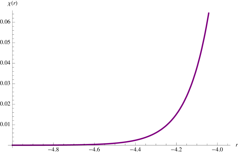
(a) Solution for $\chi$

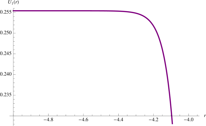
(b) Solution for $U_{1}$

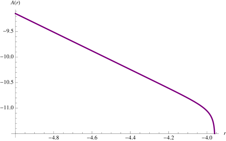
(c) Solution for $A$

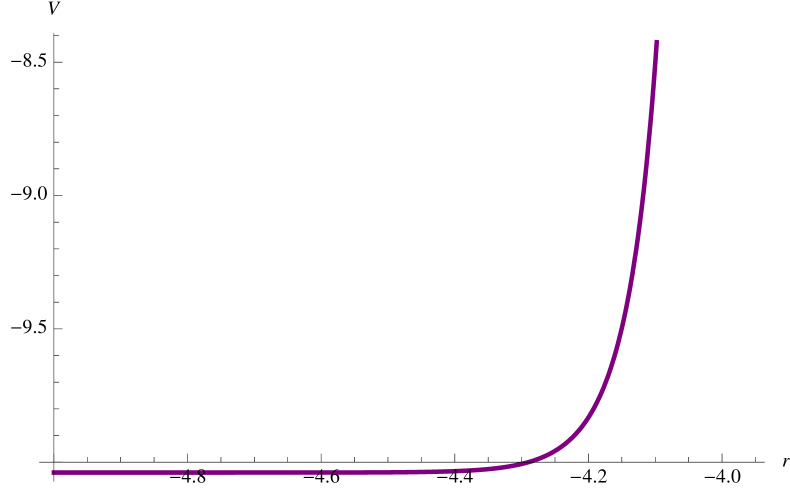
(d) The scalar potential along the flow

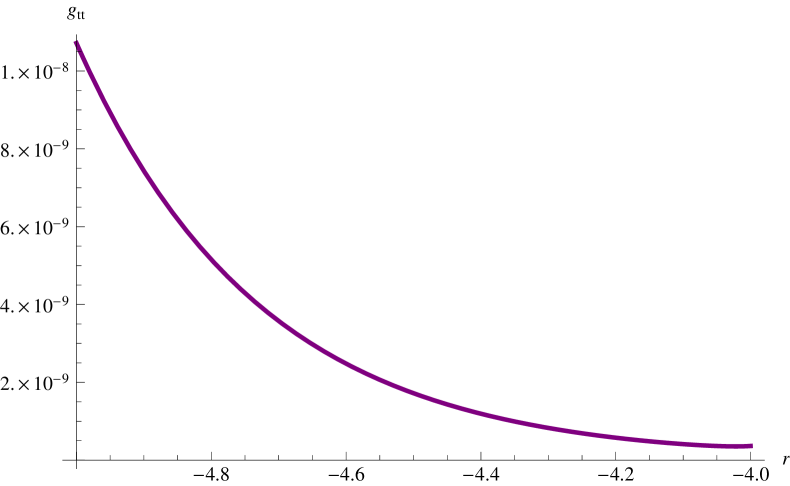
(e) The metric component $g^{(11)}_{00}$

Figure 1: An RG flow solution from $N=1$ non-conformal field theory to $N=1$ SCFT with one scalar and one pseudoscalar and $k=-1$

Note that we have identified the $N=1$ $AdS_{4}$ critical point at $\chi=0$ and $U_{1}=0.22541$, for $k=-1$, with the IR SCFT at $r=-\infty$. The numerical solution also gives a singularity consistent with the above analysis namely the divergence of scalars and the potential as well as the constancy of $g_{00}^{(11)}$. The eleven-dimensional solution near the singularity can be obtained as follow

$$ds^{2}_{11} = dx^{2}_{1,2}+dR^{2}+\left(\frac{2R}{3}\right)^{2}\left[ds^{2}(B_{\textrm{QK}})+\frac{1}{5}\eta^{I}\eta^{I}\right],$$

$$G_{4} = -6k\left(\frac{2R}{9}\right)^{\frac{7}{2}}dx^{0}\wedge dx^{1}\wedge dx^{2}\wedge dr+60\left(\frac{2R}{9}\right)^{-4}\textrm{vol}(B_{\textrm{QK}})$$ (120)

$$+6\left(\frac{2R}{9}\right)^{-4}\epsilon_{IJK}\eta^{I}\wedge\eta^{J}\wedge J^{K}-\left(\frac{2}{9}\right)^{-\frac{17}{2}}R^{-5}dR\wedge\eta^{1}\wedge\eta^{2}\wedge\eta^{3}$$

$$-5\left(\frac{2}{9}\right)^{-\frac{17}{2}}R^{-5}dR\wedge\eta^{I}\wedge J^{I}$$

where we have defined a new coordinate $R=\frac{9}{2}r^{\frac{2}{9}}$.
We now look at the most general flow solution with all four scalars turned on. The BPS equations are too complicated to be solved analytically. In any case, numerical solutions can be obtained by suitable boundary conditions similar to the previous case. From the asymptotic behaviour of these scalars given in (108), there could be many possible singularities at the end of the flows due to the presence of various vacuum expectation values (vev) and operator deformations as in the solutions studied in [24]. We will only give an example of these solutions. This is shown in figure 2 in which we take $k=-1$, and the $N=1$ critical point corresponds to the values of the scalar fields

$$U_{1}=0.25541,\qquad V_{1}=-0.45134,\qquad Z=\chi=0\,.$$ (121)

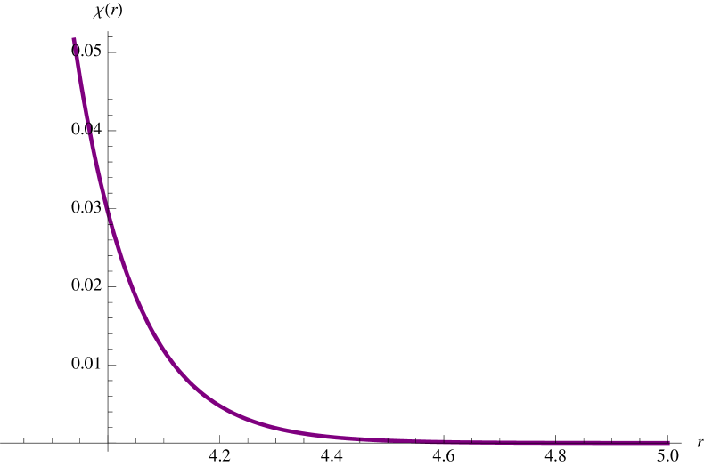
(a) Solution for $\chi$

(b) Solution for $Z$

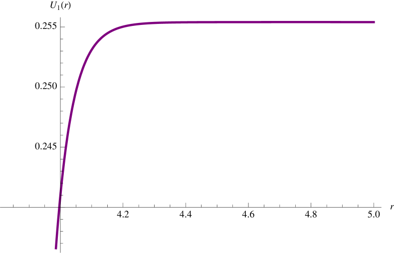
(c) Solution for $U_{1}$

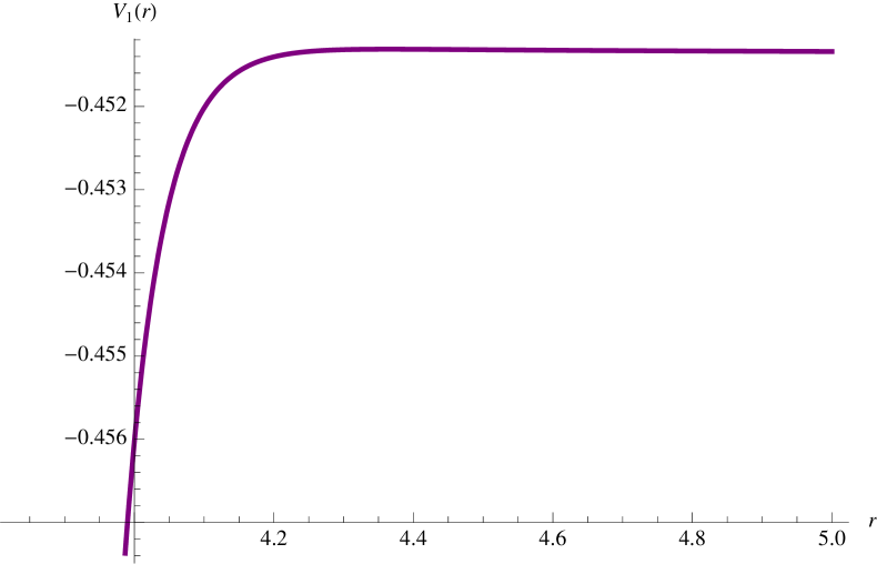
(d) Solution for $V_{1}$

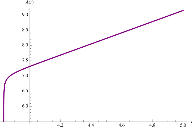
(e) Solution for $A$

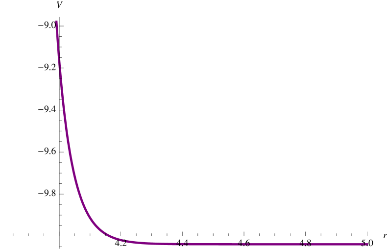
(f) The scalar potential along the flow

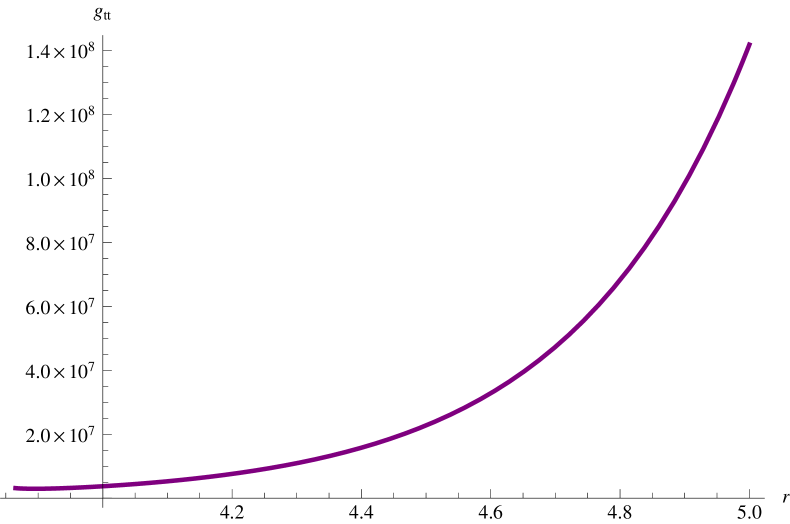
(g) The metric component $g^{(11)}_{00}$

Figure 2: An RG flow solution from $N=1$ SCFT to $N=1$ non-conformal field theory with two scalars and two pseudoscalars and $k=-1$

Near the singularity, we can see that $\chi\sim Z\rightarrow\infty$ and $U_{1}\sim V_{1}\rightarrow-\infty$. From the BPS equations, we can make an analysis near this limit resulting in the asymptotic behavior

$$U_{1}\sim 3V_{1}\sim\frac{1}{2}\ln\chi^{-\frac{3}{2}},\qquad Z\sim 5\chi\sim r^{-\frac{8}{9}}\,.$$ (122)

Using these expressions or the numerical analysis in figure 2, we can see that the singularity is physical due to the constancy of $g^{(11)}_{00}$ although the scalar potential becomes infinite. The uplift of this solution can be obtained along the same line as in the previous case.

4.2 Domain wall solutions

Similar to the $N=3$ case, we will consider $N=1$ domain wall solutions to the BPS equations with $k=0$. All of the relevant BPS equations can be obtained from those given above by setting $k=0$, so we will not repeat them here.
In the case of vanishing pseudoscalars, we find a domain wall solution to equations (98), (99) and (100) with $k=0$

$$\tilde{U} = \frac{3}{2}\tilde{V}-\frac{21}{20}\ln\left[105e^{\tilde{V}}-21\right],\qquad A=\frac{1}{2}\tilde{U},$$

$$r = \frac{2e^{\frac{1}{4}\tilde{V}}\left[2+25e^{\tilde{V}}-2\left(1-5e^{\tilde{V}}\right)^{\frac{27}{20}}\phantom{}_{2}F_{1}\left(\frac{1}{4},\frac{7}{20},\frac{5}{4},5e^{\tilde{V}}\right)\right]}{3969(21)^{\frac{7}{20}}\left(5e^{\tilde{V}}-1\right)^{\frac{27}{20}}}\,.$$ (123)

The last equation implicitly gives the scalar $\tilde{V}(r)$.
With non-vanishing pseudoscalars, we find an analytic solution only for the subtruncation to irrelevant scalars, $V_{1}=\frac{1}{3}U_{1}-\frac{1}{3}\ln 5$ and $Z=5\chi$. The solution to equations (110), (111) and (112) with $k=0$ is given by

$$U_{1} = \frac{1}{2}\ln\left[\frac{C_{1}}{2\chi^{\frac{3}{2}}}-25\chi^{2}\right],$$

$$A = \frac{1}{4}\left(50\chi^{\frac{7}{2}}-C_{1}\right)-\frac{7}{8}\ln\chi,$$

$$r = \frac{2\sqrt{5}2^{\frac{1}{4}}(C_{1}-50\chi^{\frac{7}{2}})+525\chi^{\frac{13}{8}}\left(50\chi^{\frac{7}{2}}-C_{1}\right)^{\frac{1}{4}}\phantom{}_{2}F_{1}\left(-\frac{1}{7},\frac{1}{4},\frac{6}{7},\frac{C_{1}}{50\chi^{\frac{7}{2}}}\right)}{54\chi^{\frac{9}{8}}(C_{1}-50\chi^{\frac{7}{2}})^{\frac{1}{4}}}\,.\qquad$$ (124)

When uplifted to eleven dimensions, these solutions will provide domain walls with internal four-form fluxes. All of these solutions should describe non-conformal $N=1$ field theories in three dimensions according to the DW/QFT correspondence [47, 48].

4.3 Janus solutions

In the case of $N=1$ supersymmetry, it is possible to have a supersymmetric Janus solution describing a conformal interface within the three-dimensional $N=1$ SCFT. The resulting BPS equations for an $AdS_{3}$-sliced domain wall metric can be written as

$$U_{1}^{\prime} = -\frac{2}{3}\frac{A^{\prime}}{W_{1}}\frac{\partial W_{1}}{\partial U_{1}}-\frac{2}{3}\kappa e^{U_{1}}\left(\frac{e^{-A}}{\ell W_{1}}\right)\frac{\partial W_{1}}{\partial Z},$$ (125)

$$Z^{\prime} = -\frac{2}{3}\frac{A^{\prime}}{W_{1}}e^{2U_{1}}\frac{\partial W_{1}}{\partial Z}+\frac{2}{3}\kappa e^{U_{1}}\left(\frac{e^{-A}}{\ell W_{1}}\right)\frac{\partial W_{1}}{\partial U_{1}},$$ (126)

$$V_{1}^{\prime} = -\frac{4}{9}\frac{A^{\prime}}{W_{1}}\frac{\partial W_{1}}{\partial V_{1}}-\frac{4}{3}\kappa e^{3V_{1}}\left(\frac{e^{-A}}{\ell W_{1}}\right)\frac{\partial W_{1}}{\partial\chi},$$ (127)

$$\chi^{\prime} = -4e^{6V_{1}}\frac{A^{\prime}}{W_{1}}\frac{\partial W_{1}}{\partial\chi}+\frac{4}{3}\kappa e^{3V_{1}}\left(\frac{e^{-A}}{\ell W_{1}}\right)\frac{\partial W_{1}}{\partial V_{1}},$$ (128)

$${A^{\prime}}^{2} = W_{1}^{2}-\frac{e^{-2A}}{\ell^{2}}\,.$$ (129)

These equations reduce to the RG flow equations in the limit $\ell\rightarrow\infty$ as expected. They take a very similar form to the equations studied within the $N=8$ and $N=3$ gauged supergravities in [26] and [27]. All of these equations satisfy the corresponding second-order field equations. We will not present the explicit form of these equations here due to their complexity. This can be obtained from the above equations by taking the superpotential $W_{1}$ from equation (85).
There is however a consistent truncation that can be performed by keeping only the irrelevant deformations. It can be straightforwardly checked that setting $V_{1}=\frac{U_{1}}{3}-\frac{1}{3}\ln 5$ and $Z=5\chi$ is a consistent truncation for both the above BPS equations and the corresponding field equations. The resulting equations are given by

$$U_{1}^{\prime} = \frac{2A^{\prime}}{\mathcal{Y}}\left[21e^{4U_{1}}+50ke^{2U_{1}}+25k^{2}+1750\chi^{2}(e^{2U_{1}}-k)+30625\chi^{4}\right]$$ (130)

$$-\frac{40\kappa\chi e^{-A+U_{1}}}{\ell\mathcal{Y}}(7e^{2U_{1}}+175\chi^{2}-5k),$$

$$\chi^{\prime} = -\frac{2\kappa e^{-A+U_{1}}}{5\ell\mathcal{Y}}\left[21e^{4U_{1}}+50e^{2U_{1}}+25k^{2}+1750\chi^{2}(e^{2U_{1}}-k)+30625\chi^{4}\right]$$ (131)

$$-\frac{8A^{\prime}\chi e^{2U_{1}}}{\mathcal{Y}}(7e^{2U_{1}}+175\chi^{2}-5k),$$

$$A^{\prime 2} = \frac{9}{20}e^{-7U_{1}}\left[(7e^{U_{1}}+5k^{2})^{2}+350\chi^{2}(7e^{2U_{1}}-5k)+30625\chi^{4}\right]-\frac{e^{-2A}}{\ell^{2}}$$ (132)

where $\mathcal{Y}$ is defined by

$$\mathcal{Y}=(7e^{U_{1}}+5k^{2})^{2}+350\chi^{2}(7e^{2U_{1}}-5k)+30625\chi^{4}\,.$$ (133)

Even within this simpler truncation, it is not possible to find any analytic solutions.
We now return to the BPS equations for all $SO(3)$ singlet scalars. As in the $N=8$ gauged supergravity case, these BPS equations have a turning point at which $A^{\prime}=0$. Also, the regular Janus solution is required to approach the $N=1$ $AdS_{4}$ critical point as $r\rightarrow\pm\infty$. As discussed in [26], for a given branch of $A^{\prime}$ near one of these limits, the first term in the scalar flow equations dominates. When the solution moves from the critical point, the second term will make the solution begin to loop around. At the point when $A^{\prime}=0$, the other branch of $A^{\prime}$ equation will bring the solution back to the $AdS_{4}$ critical point. The solution preserves $N=(1,0)$ or $N=(0,1)$ supersymmetry on the two dimensional-interface depending on the sign of $\kappa$.
However, from an intensive numerical search, we have not found this type of solutions even starting from $A^{\prime\prime}>0$ at the turning point. All of the solutions we obtain are singular on both sides of the turning point. Example of these solutions for the two-scalar truncation and all four scalars are shown respectively in figures 3 and 4. Note that the singularities appearing at both ends correspond to the non-conformal phases of the dual $N=1$ SCFT studied in the previous section. These are also physical singularities according to the criterion of [43]. Therefore, we expect that these singular solutions might give some physical insight to the dual $N=1$ field theories.

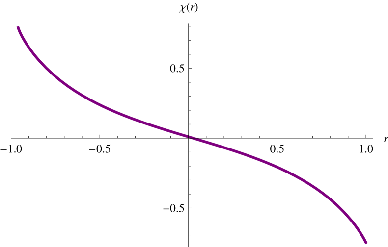
(a) Solution for $U_{1}$

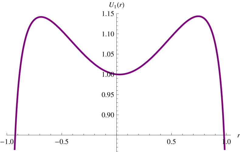
(b) Solution for $U_{1}$

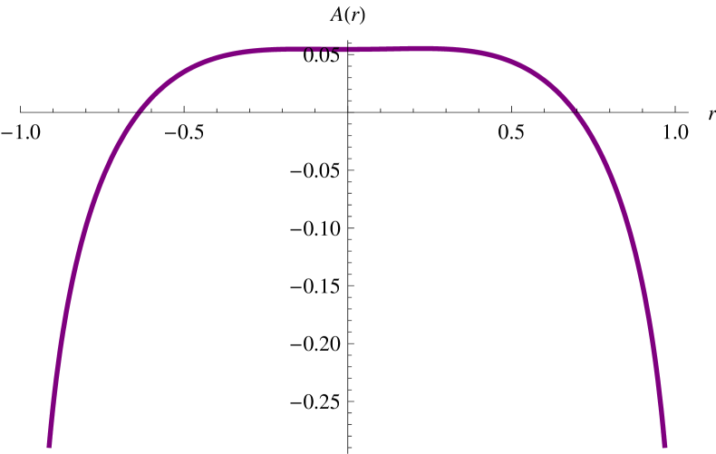
(c) Solution for $A$

Figure 3: $N=1$ Janus solution within a truncation to two irrelevant scalars with $k=-1$, $\kappa=1$ and $\ell=1$

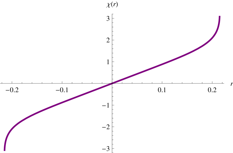
(a) Solution for $\chi$

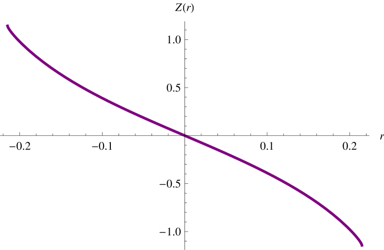
(b) Solution for $Z$

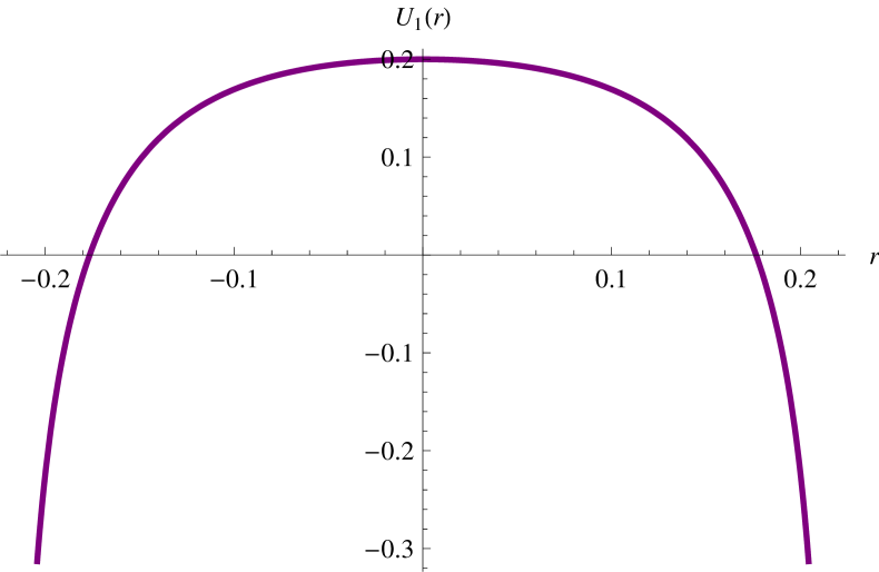
(c) Solution for $U_{1}$

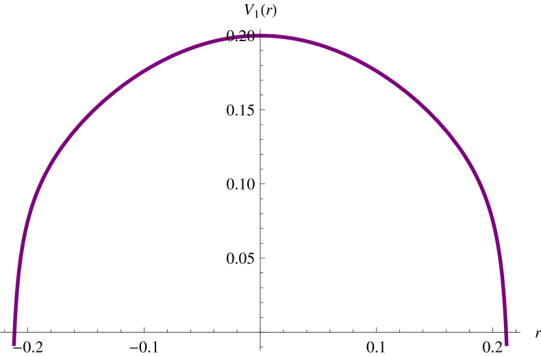
(d) Solution for $V_{1}$

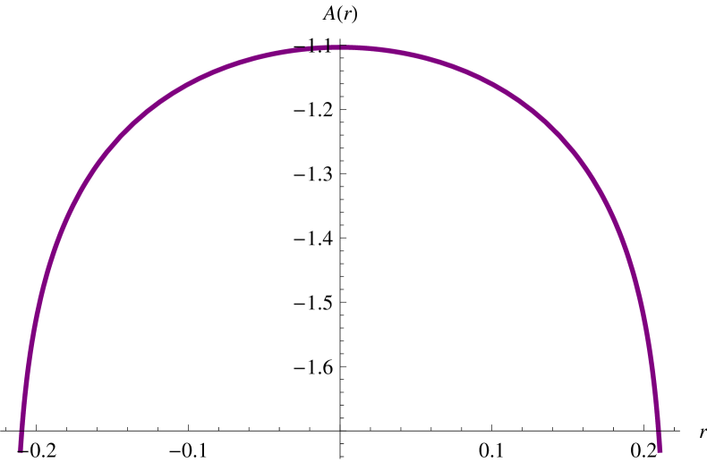
(e) Solution for $A$

Figure 4: $N=1$ Janus solution with all $SO(3)$ singlet scalars and $k=-1$, $\kappa=1$ and $\ell=1$

5 Conclusions

We have studied $N=4$ gauged supergravity in four dimensions with $SO(3)\ltimes(\mathbf{T}^{3},\hat{\mathbf{T}}^{3})$ gauge group. This theory is a consistent truncation of eleven-dimensional supergravity on a tri-sasakian manifold including massive Kaluza-Klein modes. The theory admits two supersymmetric $AdS_{4}$ critical points with $N=3$ and $N=1$ supersymmetries and unbroken $SO(3)_{R}$ R-symmetry. We have fully analyzed the BPS equations for both cases and checked that they satisfy all the second-order field equations. This analysis has not been carried out in the truncation given in [33] in which only the structure of the supermultiplets has been discussed. The result obtained in this paper is consistent with all the expectations in [33] and in a sense could be viewed as an extension of the analysis in [33] to include the fermionic supersymmetry variations.
We have subsequently used these BPS equations to study possible sueprsymmetric deformations of the dual three-dimensional $N=3$ and $N=1$ SCFTs. These deformations correspond to turning on scalar composite operators dual to the massive gravitino multiplet of the gauged supergravity or their vacuum expectation values. We have studied a number of RG flows between these SCFTs and non-conformal field theories in three dimensions. Many of these deformations lead to various singularities corresponding to possible non-conformal phases of the dual SCFTs. We have also checked that all of the new $N=1$ flow solutions presented here flow to physical singularities. Among the various solutions found in this paper, we have recovered the $N=3$ flow from $E^{1,2}\times HK$ to $AdS_{4}\times N^{010}$ and the $N=1$ flow from $E^{1,2}\times Spin(7)$ to $AdS_{4}\times\tilde{S}^{7}$ studied in [44].
The results given here provide additional gravity solutions to AdS₄/CFT₃ correspondence and might be useful in many studies along this line. In addition, we have found a number of supersymmetric domain wall solutions which might be useful in the context of DW/QFT correspondence. All of these solutions can be straightforwardly uplifted to eleven dimensions. The corresponding prescription of the uplift has also been given. It could be interesting to further study the implications of these solutions in the dual $N=1$ SCFT and $N=1$ gauge theory. The interpretation of these solutions in terms of M-brane geometries when uplifted to eleven dimensions also deserves further investigation.
Furthermore, we have looked at possible supersymmetric Janus solutions. In the $N=3$ case, this type of solutions is not possible at least with unbroken $SO(3)_{R}$ symmetry. This is similar to the five-dimensional Janus solution with unbroken $SO(6)$ symmetry [49]. There could also be non-supersymmetric Janus solutions in this case as well. For the $N=1$ case, the supersymmetric Janus solution is possible numerically. This solution corresponds to a two-dimensional conformal interface with $N=(1,0)$ unbroken supersymmetry. We have given examples of numerical Janus solutions between $N=1$ non-conformal phases of three-dimensional SCFTs. These solutions might be useful in the context of interfaced and boundary CFTs [50]. It would be interesting (if possible) to look for regular Janus solutions interpolating between $N=1$ $AdS_{4}$ critical points which describe defected CFTs in three dimensions [51].
We end the paper by pointing out other possible future works. First of all, it is interesting to consider more general solutions with a residual symmetry less than $SO(3)_{R}$. From the $N=1$ BPS equations studied here, it could be readily seen that this analysis would be very complicated. Alternatively, we could consider solutions with non-vanishing gauge fields that interpolate between $N=1,3$ $AdS_{4}$ solutions to $AdS_{2}\times\Sigma_{2}$ in which $\Sigma_{2}$ is a Riemann surface. These solutions should correspond to twisted three-dimensional SCFTs and would be interesting in the study of black hole physics. Another issue, which should be of much interest, is to construct a more general and complete truncation of eleven-dimensional supergravity on $N^{010}$. The truncation given in [33] has taken into account only $SU(3)$ singlet fields. This more general truncation could be used to uplift the RG flows and Janus solutions studied in [37] and [27] resulting in new holographic solutions in eleven dimensions. Finally, by taking the Betti multiplet into account, it would be interesting to study baryon states corresponding to M5-branes wrapped on supersymmetric $5$-cycles of $N^{010}$ similar to the study of the four-dimensional gauge theory in [52].
Acknowledgement
The author is very much indebted to Davide Cassani for various useful correspondences and clarifications on the tri-sasakian truncation. He would also like to thank Hamburg University for hospitality while some parts of this work have been done. Many discussions with Carlos Nunez are gratefully acknowledged. This work is partially supported by the German Science Foundation (DFG) under the Collaborative Research Center (SFB) 676 “Particles, Strings and the Early Universe” and The Thailand Research Fund (TRF) under grant RSA5980037.

Appendix A Field equations for $SO(3)_{R}$ singlet scalars

In this appendix, we explicitly give the field equations for all of the four $SO(3)_{R}$ singlet scalars and the corresponding Einstein equations. Since the equations in the RG flow case can be obtained from those of the Janus solutions, we will only give the equations for the Janus solutions.
The scalar equations are given by

$$U_{1}^{\prime\prime}+3A^{\prime}U_{1}^{\prime}-e^{-6U_{1}-3V_{1}}\left[2e^{4U_{1}}+24e^{3U_{1}+3V_{1}}-8e^{2U_{1}+6V_{1}}-18k^{2}\right.$$

$$-4Z^{2}(2e^{2U_{1}}+18e^{6V_{1}}-9k)-18Z^{4}-8\chi^{2}(e^{2U_{1}}+9Z^{2})$$

$$\left.-8\chi Z(2e^{2U_{1}}-9k+9Z^{2})-Z^{\prime 2}e^{4U_{1}+3V_{1}}\right] = 0,$$ (134)

$$V_{1}^{\prime\prime}+3A^{\prime}V_{1}^{\prime}-\frac{1}{3}e^{-6U_{1}-6V_{1}}\left[6e^{4U_{1}+3V_{1}}+12e^{2U_{1}+9V_{1}}-18k^{2}e^{3V_{1}}\right.$$

$$+12e^{3V_{1}}Z^{2}(6e^{6V_{1}}-e^{2U_{1}}+3k)-24\chi Ze^{3V_{1}}(e^{2U_{1}}-3k+3Z^{2})$$

$$\left.-18Z^{4}e^{3V_{1}}-12\chi^{2}e^{3V_{1}}(e^{2U_{1}}+6Z^{2})-\chi^{\prime 2}e^{6U_{1}}\right] = 0,$$ (135)

$$\chi^{\prime\prime}+3A^{\prime}\chi^{\prime}-6\chi^{\prime}V_{1}^{\prime}-6e^{-6U_{1}+3V_{1}}\left[4e^{2U_{1}}(\chi+Z)\right.$$

$$\left.+12Z(Z^{2}+2\chi Z-k)\right] = 0,$$ (136)

$$Z^{\prime\prime}+3A^{\prime}Z^{\prime}-2U_{1}^{\prime}Z^{\prime}-4e^{-4U_{1}-3V_{1}}\left[Z(e^{2U_{1}}+6e^{6V_{1}}-3k+3Z^{2})\right.$$

$$\left.+6\chi^{2}Z+\chi(e^{2U_{1}}-3k+9Z^{2})\right] = 0\,.$$ (137)

With the metric ansatz (37), the Einstein equations give rise to the following (dependent) equations

$$2A^{\prime\prime}+3{A^{\prime}}^{2}+\frac{e^{-2A}}{\ell^{2}}+\frac{3}{2}{U_{1}^{\prime}}^{2}+\frac{9}{4}{V^{\prime}_{1}}^{2}+\frac{1}{4}e^{-6V_{1}}{\chi^{\prime}}^{2}+\frac{3}{2}e^{-2U_{1}}{Z^{\prime}}^{2}+V = 0,\,\,\,\,$$ (138)

$$3{A^{\prime}}^{2}+\frac{3}{\ell^{2}}e^{-2A}-\frac{3}{2}{U_{1}^{\prime}}^{2}-\frac{9}{4}{V_{1}^{\prime}}^{2}-\frac{1}{4}e^{-6V_{1}}{\chi^{\prime}}^{2}-\frac{3}{2}e^{-2U_{1}}{Z^{\prime}}^{2}+V = 0$$ (139)

where $V$ is the scalar potential given in (56).

Appendix B BPS equations for $N=1$ supersymmetry

We give the BPS equations for the $N=1$ RG flow solutions here. These equations are given by

$$U_{1}^{\prime} = \frac{e^{-\frac{3}{2}(2U_{1}+V_{1})}}{\mathcal{Q}}\left[(e^{2U_{1}}+2e^{U_{1}+3V_{1}}+k)(e^{2U_{1}}+4e^{U_{1}+3V_{1}}+3k)\right.$$ (140)

$$+2Z^{2}(2e^{2U_{1}}+6e^{6V_{1}}+5e^{U_{1}+3V_{1}}-3k)+4\chi^{2}(2e^{2U_{1}}+3Z^{2})$$

$$\left.+3Z^{4}+4\chi Z(2e^{2U_{1}}+3Z^{2}-3k)\right],$$

$$V_{1}^{\prime} = \frac{e^{-\frac{3}{2}(2U_{1}+V_{1})}}{\mathcal{Q}}\left[(e^{2U_{1}}+k)^{2}-4e^{2U_{1}+6V_{1}}+2Z^{2}(e^{2U_{1}}-2e^{6V_{1}}-k)\right.$$ (141)

$$\left.+Z^{4}+4\chi^{2}(e^{2U_{1}}+Z^{2})+4\chi Z(e^{2U_{1}}+Z^{2}-k)\right],$$

$$Z^{\prime} = -\frac{2e^{-U_{1}-\frac{3}{2}V_{1}}}{\mathcal{Q}}\left[2Ze^{6V_{1}}+2Ze^{U_{1}+3V_{1}}+(\chi+Z)(e^{2U_{1}}+2\chi Z+Z^{2}-k)\right],$$

$$\chi^{\prime} = -\frac{12e^{-3U_{1}+\frac{9}{2}V_{1}}}{\mathcal{Q}}\left[(2\chi+Z)e^{2U_{1}}+Z(Z^{2}+2\chi Z-k)\right]$$ (143)

where

$$\mathcal{Q}=\sqrt{\left[2e^{3V_{1}}Z+2(\chi+Z)e^{U_{1}}\right]^{2}+\left[e^{2U_{1}}+2e^{U_{1}+3V_{1}}+k-Z(2\chi+Z)\right]^{2}}\,.$$ (144)

References

- [1] J. M. Maldacena, “The large limit of superconformal field theories and supergravity”, Adv. Theor. Math. Phys. 2 (1998) 231-252, arXiv: hep-th/9711200.
- [2] J. Bagger and N. Lambert, “Gauge Symmetry and Supersymmetry of Multiple M2-Branes”, Phys. Rev. D77 (2008) 065008, arXiv: 0711.0955.
- [3] O. Aharony, O. Bergman, D. L. Jafferis and J. Maldacena, “ superconformal Chern-Simons-matter theories, M2-branes and their gravity duals”, JHEP 10 (2008) 091, arXiv: 0806.1218.
- [4] J. P. Gauntlett, J. Sonner, T. Wiseman, “Holographic superconductivity in M-Theory”, Phys. Rev. Lett. 103 (2009) 151601, arXiv: 0907.3796.
- [5] S. S. Gubser, S. S. Pufu and F. D. Rocha, “Quantum critical superconductors in string theory and M-theory”, Phys. Lett. B683 (2010) 201-204, arXiv: 0908.0011.
- [6] J. P. Gauntlett, J. Sonner, T. Wiseman, “Quantum Criticality and Holographic Superconductors in M-theory”, JHEP 02 (2010) 060, arXiv: 0912.0512.
- [7] D.Z. Freedman, S. Gubser, N. Warner and K. Pilch, “Renormalization Group Flows from Holography-Supersymmetry and a c-Theorem”, Adv. Theor. Math. Phys. 3 (1999). arXiv: hep-th/9904017.
- [8] Alexei Khavaev and Nicholas P. Warner, “A Class of Supersymmetric RG Flows from Five-dimensional Supergravity”, Phys. Lett. 495 (2000) 215-222. arXiv: hep-th/0009159.
- [9] L.Girardello, M.Petrini, M.Porrati and A. Zaffaroni, “Novel Local CFT and exact results on perturbations of super Yang-Mills from AdS dynamics”, JHEP 9812 (1998) 022, arXiv: hep-th/9810126.
- [10] D. Bak, M. Gutperle and S. Hirano, “A Dilatonic Deformation of and its Field Theory Dual”, JHEP 05 (2003) 072, arXiv: hep-th/0304129.
- [11] A. B. Clark, D. Z. Freedman, A. Karch and M. Schnabl, “Dual of the Janus solution: An interface conformal field theory”, Phys. Rev. D71 (2005) 066003, arXiv: hep-th/0407073.
- [12] E. D’ Hoker, J. Estes and M. Gutperle, “Interface Yang-Mills, supersymmetry, and Janus”, Nucl. Phys. B753 (2006) 16, arXiv: hep-th/0603013.
- [13] D. Gaiotto and E. Witten, “Janus Configurations, Chern-Simons Couplings, And The thetaAngle in N=4 Super Yang-Mills Theory”, JHEP 1006 (2010) 097, arXiv: 0804.2907.
- [14] O. DeWolfe, D. Z. Freedman and H. Ooguri, “Holography and Defect Conformal Field Theories”, Phys. Rev. D66 (2002) 025009, arXiv: hep-th/0111135.
- [15] A. Clark and A. Karch, “Super Janus”, JHEP 10 (2005) 094, arXiv: hep-th/0506265.
- [16] M. W. Suh, “Supersymmetric Janus solutions in five and ten dimensions”, JHEP 09 (2011) 064, arXiv: 1107.2796.
- [17] C. Ahn and J. Paeng, “Three-Dimensional SCFTs, Supersymmetric Domain Wall and Renormalization Group Flow”, Nucl. Phys. B595 (2001) 119-137, arXiv: hep-th/0008065.
- [18] C. Ahn and K. Woo, “Supersymmetric Domain Wall and RG Flow from 4-Dimensional Gauged Supergravity”, Nucl. Phys. B599 (2001) 83-118, arXiv: hep-th/0011121.
- [19] C. Ahn and T. Itoh, “An Supersymmetric -invariant Flow in M-theory”, Nucl. Phys. B627 (2002) 45-65, arXiv: hep-th/0112010.
- [20] N. Bobev, N. Halmagyi, K. Pilch and N. P. Warner, “Holographic, Supersymmetric RG Flows on M2 Branes”, JHEP 09 (2009) 043, arXiv: 0901.2376.
- [21] T. Fischbacher, K. Pilch and N. P. Warner, “New Supersymmetric and Stable, Non-Supersymmetric Phases in Supergravity and Holographic Field Theory”, arXiv: 1010.4910.
- [22] A. Guarino, “On new maximal supergravity and its BPS domain-walls”, JHEP 02 (2014) 026, arXiv: 1311.0785.
- [23] J. Tarrio and O. Varela, “Electric/magnetic duality and RG flows in ”, JHEP 01 (2014) 071, arXiv: 1311.2933.
- [24] Y. Pang, C. N. Pope and J. Rong, “Holographic RG Flow in a New Sector of -Deformed Gauged Supergravity”, JHEP 08 (2015) 122, arXiv: 1506.04270.
- [25] K. Pilch, A. Tyukov and N. P. Warner, “ Supersymmetric Janus Solutions and Flows: From Gauged Supergravity to M Theory”, JHEP 05 (2016) 005, arXiv: 1510.08090.
- [26] N. Bobev, K. Pilch and N. P. Warner, “Supersymmetric Janus Solutions in Four Dimensions”, JHEP 1406 (2014) 058, arXiv: 1311.4883.
- [27] P. Karndumri, “Supersymmetric Janus solutions in four-dimensional gauged supergravity”, Phys. Rev. D93 (2016) 125012, arXiv: 1604.06007.
- [28] L. Castellani and L.J. Romans, “ and Supersymmetry in a New Class of Solutions for Supergravity”, Nucl. Phys. B238 (1984) 683-701.
- [29] P. Termonia, “The complete Kaluza Klein spectrum of 11D supergravity on ”, Nucl. Phys. B577 (2000) 341-389, arXiv: hep-th/9909137.
- [30] P. Fre, L. Gualtieri and P. Termonia, “The structure of multiplets in and the complete spectrum of M-theory on ”, Phys. Lett. B471 (1999) 27-38, arXiv: hep-th/9909188.
- [31] M. Billo, D. Fabbri, P. Fre, P. Merlatti and A. Zaffaroni, “Rings of short superfields in three dimensions and M-theory on ”, Class. Quant. Grav. 18 (2001) 1269-1290, arXiv: hep-th/0005219.
- [32] M. Billo, D. Fabbri, P. Fre, P. Merlatti and A. Zaffaroni, “Shadow multiplets in and the super-Higgs mechanism: hints of new shadow supergravities”, Nucl. Phys. B591 (2000) 139-194, arXiv: hep-th/0005220.
- [33] D. Cassani and P. Koerber, “Tri-Sasakian consistent reduction”, JHEP 01 (2012) 086, arXiv: 1110.5327.
- [34] A. Hanany and A. Zaffaroni, “Tilings, Chern-Simons Theories and M2 Branes”, JHEP 10 (2008) 111, arXiv: 0808.1244.
- [35] A. Hanany, D. Vegh and A. Zaffaroni, “Brane Tilings and M2 Branes”, JHEP 03 (2009) 012, arXiv: 0809.1440.
- [36] H. Ooguri and C. S. Park, “Superconformal Chern-Simons theories and the squashed seven sphere”, JHEP 11 (2008) 082, arXiv: 0808.0500.
- [37] P. Karndumri, “Holographic RG flows in Chern-Simons-Matter theory from 4D gauged supergravity”, Phys. Rev. D94 (2016) 045006, arXiv: 1601.05703.
- [38] J. Schon and M. Weidner, “Gauged supergravities”, JHEP 05 (2006) 034, arXiv: hep-th/0602024.
- [39] C. Horst, J. Louis and P. Smyth, “Electrically gauged supergravities in with vacua”, JHEP 03 (2013) 144, arXiv: 1212.4707.
- [40] P. Wagemans, “Breaking of supergravity to , at , Phys. Lett. B206 (1988) 241.
- [41] L. Castellani, “On G/H geometry and its use in M-theory compactifications”, Annals Phys. 287 (2001) 1-13, arXiv: hep-th/9912277.
- [42] S. S. Gubser, “Curvature singularities: the good, the bad and the naked”, Adv. Theor. Math. Phys. 4 (2000) 679-745, arXiv: hep-th/0002160.
- [43] J. Maldacena and C. Nunez, “Supergravity description of field theories on curved manifolds and a no go theorem”, Int. J. Mod. Phys. A16 (2001) 822, arXiv: hep-th/0007018.
- [44] U. Gursoy, C. Nunez and M. Schvellinger, “RG flows from Spin(7), CY 4-fold and HK manifolds to AdS, Penrose limits and pp waves”, JHEP 06 (2002) 015, arXiv: hep-th/0203124.
- [45] C. Ahn, “Other squaching deformation and superconformal Chern-Simons gauge theory”, Phys. Lett. B671 (2009) 303-309, arXiv: 0810.2422.
- [46] C. Ahn and Soo-Jong Rey, “More CFTs and RG Flows from Deforming M2/M5-Brane Horizon”, Nucl. Phys. B572 (2000) 188-207, arXiv: hep-th/9911199.
- [47] H.J. Boonstra, K. Skenderis and P.K. Townsend, “The domain-wall/QFT correspondence”, JHEP 01 (1999) 003, arXiv: hep-th/9807137.
- [48] T. Gherghetta and Y. Oz, “Supergravity, Non-Conformal Field Theories and Brane-Worlds”, Phys. Rev. D65 (2002) 046001, arXiv: hep-th/0106255.
- [49] E. D’ Hoker, J. Estes and M. Gutperle, “Interface Yang-Mills, supersymmetry, and Janus”, Nucl. Phys. B753 (2006) 16, arXiv: hep-th/0603013.
- [50] M. Gutperle and J. Samani, “Holographic RG-flows and Boundary CFTs”, Phys. Rev. D86 (2012) 106007, arXiv: 1207.7325.
- [51] D. M. McAvity and H. Osborn, “Conformal field theories near a boundary in general dimensions”, Nucl. Phys. B455 (1995) 522, arXiv: cond-mat/9505127.
- [52] S. S. Gubser and I. R. Klebanov, “Baryons and Domain Walls in an Superconformal Gauge Theory”, Phys. Rev. 58 (1998) 125025, arXiv: hep-th/9808075.