Numerical analysis of strongly nonlinear PDEs

Abstract

We review the construction and analysis of numerical methods for strongly nonlinear PDEs, with an emphasis on convex and nonconvex fully nonlinear equations and the convergence to viscosity solutions. We begin by describing a fundamental result in this area which states that stable, consistent, and monotone schemes converge as the discretization parameter tends to zero. We review methodologies to construct finite difference, finite element, and semi-Lagrangian schemes that satisfy these criteria, and, in addition, discuss some rather novel tools that have paved the way to derive rates of convergence within this framework.

1 Introduction

Все счастливые семьи похожи друг на друга, каждая несчастливая семья несчастлива по-своему.

L. Tolstoy

The quote above from L. Tolstoy [127], which roughly translates to “All happy families resemble each other, but each unhappy one is unhappy in its own way” was used in [67, Section 8.1] to point out that the numerical approximation of partial differential equations substantially differs from that of ordinary differential equations. The same quote was used in the Preface of [65] to say that the theory for nonlinear equations is very different than the one for linear problems, and that each nonlinearity needs to be treated in its own way. For these reasons we feel compelled to begin our discussion with the same quote, since we have chosen the unhappiest of all possible families for numerical approximation: Fully nonlinear equations.

The goal of this paper is to summarize recent advances and trends in the numerical approximation and theory of strongly second-order nonlinear PDEs with an emphasis on fully nonlinear convex and nonconvex PDEs. Such PDEs appear in diverse applications such as weather and climate modeling, stochastic optimal control, determining the initial shape of the universe, optimal reflector design, differential geometry, optimal transport, mathematical finance, image processing, and mesh generation. Despite their importance in these application areas, and in contrast to the PDE and solution theory, numerical methods for fully nonlinear problems is still an emerging field in numerical analysis. The reasons for the delayed development are plentiful. Besides the strong nonlinearity, the fundamental difficulties in computing solutions of fully nonlinear problems are the lack of regularity of solutions, the conditional uniqueness of solutions, and most importantly, the notion of viscosity solutions. Similar to weak solutions for PDEs in divergence-form, the viscosity solution concept relaxes the pointwise meaning of the PDE, and while doing so, broadens the class of admissible functions in which to seek a solution. However, unlike the weak solution framework, the definition of viscosity solutions is not based on variational principles, but rather comparison principles. While viscosity solution theory and the PDE theory of fully nonlinear problems has made incredible progress during the last 25 years, the numerical results for such problems has been slow to catch up due to pointwise nature and nonvariational structure found in the theory.

A breakthrough occurred in 1991 with [8] which roughly speaking, asserts that a consistent, stable and monotone numerical method (or general approximation scheme) converges to the viscosity solution as the discretisation or regularization parameter tends to zero. The first two conditions in this framework, consistency and stability, are expected; they are the cornerstone of any convergence theory of numerical PDEs and is recognized as the basis of the Lax-Richtmyer equivalence theorem. While arguably less well-known, monotonicity of numerical methods is also a long-established area of study, for example, its importance in the context of linear finite difference schemes has been realized (at least) 80 years ago (see, e.g., [57, 101]). On the other hand, the construction of numerical methods that satisfy all three criteria, at least for fully nonlinear problems, is not immediately obvious.

Around the same time, and complementary to the Barles-Souganidis framework, [88, 89] gave a methodology to construct consistent, stable, and monotone finite difference schemes for uniformly elliptic fully nonlinear operators. In addition, they showed that such discrete schemes satisfy properties found in the viscosity solution theory, including Alexandrov-Bakelman-Pucci (ABP) maximum principles, Harnack inequalities, and Hölder estimates. While these results gave a somewhat practical guide to compute viscosity solutions, and the theory paved the way for future advancements, the fundamental issue of convergence rates was explicitly stated as an open and elusive problem.

For the next 15 years progress of numerical fully nonlinear second-order PDEs was relatively limited and mostly constrained to the theory and convergence rates for convex PDEs, in particular, the Hamilton-Jacobi-Bellman equation. In this direction, [80] introduced the groundbreaking idea of “shaking the coefficients” to obtain sufficiently smooth subsolutions, which along with comparison principles, yield rates of convergence even for degenerate problems. These techniques were later refined under various scenarios and assumptions of the problem and discretisation (e.g., [6, 7, 85]), although convexity of the equation always played an essential role in the analysis.

The last ten years has seen an explosion of results for numerical nonlinear PDEs, including a variety of discretization types and convergence results. These include the construction of relatively simple and practical wide-stencil finite difference schemes tailored to specific PDEs [114, 54, 13, 53], and the emergence of Galerkin methods for fully nonlinear problems [49, 47, 46, 34, 35]. With regard to the convergence theory, [26], using intricate regularity results, derived algebraic rates of convergence for finite difference approximations for nonconvex PDEs with constant coefficients, and these results were quickly extended to problems with variable coefficients and lower-order terms by [82] and [131]. On the Galerkin front, [109] extended the Kuo-Trudinger theory to finite element methods and derived ABP maximum principles for linear elliptic problems. These results were soon extended in several directions, including rates of convergence for a discrete Monge-Ampère equation [112] and wide-stencil finite difference schemes [110], and the construction and analysis of finite element methods for nonconvex fully nonlinear problems [119].

The intention of this survey is to summarize the 25 years of development of fully nonlinear numerical PDEs. Let us describe the organization and the problems we consider in the paper. After setting the notation and stating some instances of fully nonlinear problems, we review some of the basic theory and analysis of elliptic PDEs in Section 2. Here different notions of solutions are introduced and the underlying properties of the solutions and operators are discussed. Besides being of independent interest these fundamental results motivate both the construction and analysis of the numerical methods. We develop a general framework to compute second-order elliptic problems in Section 3. Basic properties of numerical methods, namely, consistency, stability, and monotonicity are given, which will lay the groundwork for future developments in the paper. Special attention will be on discrete ABP maximum principles in both the finite difference and finite element setting. Section 4 concerns finite element approximations for linear problems in non-divergence form and with nonsmooth coefficients. In Section 5 we combine the ideas of the previous sections and consider finite element and finite difference approximations for fully nonlinear convex PDEs. Besides the construction and convergence of the schemes, a focus of this section is the rates of convergence and the techniques to obtain these results. These results are extended to a particular convex PDE, the Monge-Ampère equation, in Section 6. We discuss recent results of the numerical approximations for fully nonlinear nonconvex PDEs in Section 7. Finally we give some concluding remarks and state some open problems in Section 8.

Before starting our discussion let us first briefly outline the derivation of some fully nonlinear PDEs that we focus on in the paper and illustrate their connection with some applications and other areas of mathematics.

1.1 Convex PDEs

This section obtains an instance of the Hamilton-Jacobi-Bellman (HJB) equation, a prototypical fully nonlinear second-order convex PDE, and shows how such problems arise in stochastic optimal control problems. In addition, we show below that every uniformly elliptic, convex operator with bounded gradient is an implicit HJB problem.

Following [115, Chapter 11] and [51], we consider a stochastic process $X_{\tau}$ governed by the differential equation

$$\begin{dcases}dX_{\tau}=\ell(X_{\tau},\tau,\alpha_{\tau})\,\mbox{\rm d}\tau+{\sigma}(X_{\tau},\tau,\alpha_{\tau})\,\mbox{\rm d}W_{\tau}\quad\tau>0,\\ X_{0}=x_{0}\in\mathbb{R}^{d}.\end{dcases}$$ (1.1)

Here, $W_{\tau}$ is a Brownian motion of dimension $d$, $\sigma$ is an $d\times d$ matrix-valued function, $\alpha_{\tau}\in{\mathcal{A}}$ is a (Markov) control and $\mathcal{A}$ is the control space. Problem (1.1) describes a dynamical system driven by additive white noise with diffusion coefficient (or volatility) $\sigma$ and non-stochastic drift $\ell$. Under appropriate smoothness and growth conditions on $\ell$ and $\sigma$, and for a fixed $\alpha(\cdot)\in\mathcal{A}$, there is a path-wise unique solution to (1.1). Associated with problem (1.1) is the family of stochastic processes that satisfy (1.1) but with initial time $t\geq 0$:

$$\begin{dcases}\,\mbox{\rm d}X^{x,t}_{\tau}=\ell(X^{x,t}_{\tau},\tau,\alpha_{\tau})\,\mbox{\rm d}\tau+{\sigma}(X^{x,t}_{\tau},\tau,\alpha_{\tau})\,\mbox{\rm d}W_{\tau}\quad\tau>t,\\ X^{x,t}_{t}=x\in\mathbb{R}^{d},\end{dcases}$$ (1.2)

Now let $\Omega\subset\mathbb{R}^{d}$ be an open bounded domain, and set $Q=\Omega\times(0,T)$ for some $T\in(0,\infty]$. Denote by $\hat{T}$ the first exit time for the process $X^{x,t}_{\tau}$ satisfying (1.2), i.e.,

$$\hat{T}=\hat{T}^{x,t}=\inf\{\tau>t;(X^{x,t}_{\tau},\tau)\not\in Q\}.$$

We then define the performance function (or cost functional)

$$J(x,t,\alpha)=\mathbb{E}_{x,t}\Big{\{}\int_{t}^{\hat{T}}f(X^{x,t}_{\tau},\tau,\alpha_{\tau})\,\mbox{\rm d}\tau+\chi_{{\hat{T}}<\infty}\psi(X^{x,t}_{\hat{T}},\hat{T})\Big{\}}$$

over all $\alpha\in\mathcal{A}$ under the constraint (1.2). Here, $f:\mathbb{R}^{d}\times\mathbb{R}\times\mathcal{A}\to\mathbb{R}$ is the profit rate function, $\psi:\mathbb{R}^{d}\times\mathbb{R}\to\mathbb{R}$ is the bequest function, $\chi_{\hat{T}<\infty}$ is the indicator function, which equals one if $\hat{T}<\infty$ and equals zero otherwise, and $\mathbb{E}_{x,t}$ represents the expectation conditional on $X^{x,t}_{t}=x$. We then consider the problem of finding the value function $u:\bar{Q}\to\mathbb{R}$ and optimal control $\alpha^{*}\in\mathcal{A}$ such that

$$u(x,t)=\sup_{\alpha\in\mathcal{A}}J(x,t,\alpha)=J(x,t,\alpha^{*}).$$

Let us now give an heuristic derivation of the Hamilton-Jacobi-Bellman equation based on Bellman’s principle of optimality and Itô’s lemma. First, the Bellman’s principle of optimality states that [9]:

Whatever the initial state $\{X^{x,t}_{s}\}_{s<\tau}$ and initial decision $\{\alpha_{s}\}_{s<\tau}$ are, the remaining controls $\{\alpha_{s}\}_{s>\tau}$ must constitute an optimal policy with regard to the state $X^{x,t}_{\tau}$ resulting from the initial decision.

More precisely, this principle equates to

$$u(x,t)=\sup_{\alpha\in\mathcal{A}}\mathbb{E}_{x,t}\left\{u(X^{x,t}_{t+\delta t},t+\delta t)+\int_{t}^{t+\delta t}f(X^{x,t}_{\tau},\tau,\alpha_{\tau})\,\mbox{\rm d}\tau\right\}.$$ (1.3)

Next, recalling that $X^{x,t}_{t}=x$, by Itô’s lemma we obtain

$$u(X^{x,t}_{t+\delta t},t+\delta t) =u(x,t)+\int_{t}^{t+\delta t}\frac{\partial u}{\partial t}\,\mbox{\rm d}\tau+\int_{t}^{t+\delta t}Du\cdot\,\mbox{\rm d}X^{x,t}_{\tau}$$

$$\qquad+\frac{1}{2}\int_{t}^{t+\delta t}\,\mbox{\rm d}X^{x,t}_{\tau}\cdot D^{2}u\,\mbox{\rm d}X^{x,t}_{\tau}.$$

Since the state variable $X^{x,t}_{\tau}$ is governed by the stochastic equation (1.2), and by using the identity $\,\mbox{\rm d}W_{\tau}\otimes\,\mbox{\rm d}W_{\tau}=I\,\mbox{\rm d}\tau$ we obtain

$$\;u(X^{x,t}_{t+\delta t},t+\delta t)-u(x,t)$$

$$= \;\int_{t}^{t+\delta t}\left(\frac{\partial u}{\partial t}+Du\cdot\ell+\frac{1}{2}(\sigma\sigma^{\intercal}):D^{2}u\right)\,\mbox{\rm d}\tau+\int_{t}^{t+\delta t}(\sigma^{\intercal}Du)\cdot\,\mbox{\rm d}W_{\tau}.$$

Therefore, from principle of optimality (1.3),

$$\sup_{\alpha\in\mathcal{A}}\mathbb{E}_{x,t}\left\{u(X^{x,t}_{t+\delta t},t+\delta t)-u(x,t)+\int_{t}^{t+\delta t}f(X^{x,t}_{\tau},\tau,\alpha)\,\mbox{\rm d}\tau\right\}=0$$

and Itô’s formula above, we obtain

$$\sup_{\alpha\in\mathcal{A}}\mathbb{E}_{x,t}\left\{\int_{t}^{t+\delta t}\left(\frac{\partial u}{\partial t}+Du\cdot\ell+\frac{1}{2}(\sigma\sigma^{\intercal}):D^{2}u+f\right)\,\mbox{\rm d}\tau\right\}=0,$$

where we used that

$${\mathbb{E}}_{x,t}\left\{\int_{t}^{t+\delta t}(\sigma^{\intercal}Du)\cdot\,\mbox{\rm d}W_{\tau}\right\}=0.$$

Dividing by $\delta t$ and formally taking the limit $\delta t\to 0$, we then obtain a deterministic equation, namely, the Hamilton-Jacobi-Bellman equation

$$\frac{\partial u}{\partial t}(x,t)+\sup_{\alpha\in\mathcal{A}}\left(\mathcal{L}^{\alpha}u(x,t)+f(x,t,\alpha)\right)=0,$$

where

$$\mathcal{L}^{\alpha}u(x,t)=Du(x,t)\cdot\ell(x,t,\alpha)+\frac{1}{2}\sigma(x,t,\alpha)\sigma(x,t,\alpha)^{\intercal}:D^{2}u(x,t).$$

To derive the equation, we assumed that the value function $u(x,t)$ has continuous second order derivatives. However, the PDE theory reveals that the solution of the HJB equation in general does not satisfy this regularity assumption. To justify the derivation above, the concept of viscosity solutions was introduced in [32] for first order Hamilton-Jacobi equations and later generalized to second order Hamilton-Jacobi-Bellman equations [94, 95]. Viscosity solutions, which is an essential concept in the PDE theory, will also play an important role in this paper.

1.2 Nonconvex PDEs

The Isaacs equation, a prototypical nonconvex PDE, describes zero sum stochastic games with two players. Each player has one control and they have opposite objectives. The first player chooses a control to maximize the expected payoff, whereas the second player chooses a control to minimize it. Stochastic game theory has wide applications in engineering and mathematical finance. Here, we follow the ideas in [52] to derive the equation.

The dynamics of the stochastic differential game we investigate are given by the controlled stochastic differential equation

$$\begin{dcases}\,\mbox{\rm d}X^{x,t}_{\tau}=\ell(X^{x,t}_{\tau},\tau,\alpha_{\tau},\beta_{\tau})\,\mbox{\rm d}\tau+\sigma(X^{x,t}_{\tau},\tau,\alpha_{\tau},\beta_{\tau})\,\mbox{\rm d}W_{\tau}\quad\tau>t,\\ X^{x,t}_{t}=x\in\mathbb{R}^{d},\end{dcases}$$ (1.4)

and the expected payoff is

$$J(x,t,\alpha,\beta)={\mathbb{E}}_{x,t}\left\{\int_{t}^{\hat{T}}f(X^{x,t}_{\tau},\tau,\alpha_{\tau},\beta_{\tau})\,\mbox{\rm d}\tau+\chi_{\hat{T}<\infty}\psi(X^{x,t}_{\hat{T}},\hat{T})\right\},$$

where $X^{x,t}_{\tau}$ satisfies the differential equation (1.4) for $\tau>t$ and has initial condition $X^{x,t}_{t}=x$.

The Isaacs equation can be derived in a similar fashion as the HJB equation. If, at time $t$, the first player chooses a control $\alpha$ to maximize the expected payoff $J$, and the second player, based on the decision of first player, chooses the control $\beta$ to minimize it, then we set

$$u^{+}(x,t)=\inf_{\beta\in{\mathcal{B}}}\sup_{\alpha\in{\mathcal{A}}}{\mathbb{E}}_{x,t}\{J(x,t,\alpha,\beta)\},$$

and call this the upper value function. On the other hand, if the second player makes the decision first and the first player reacts accordingly, then we set the lower value function as

$$u^{-}(x,t)=\sup_{\alpha\in{\mathcal{A}}}\inf_{\beta\in{\mathcal{B}}}{\mathbb{E}}_{x,t}\{J(x,t,\alpha,\beta)\}.$$

By the principle of optimality we have

$$u^{+}(x,t)=\inf_{\beta\in{\mathcal{B}}}\sup_{\alpha\in{\mathcal{A}}}{\mathbb{E}}_{x,t}\left\{u^{+}(X^{x,t}_{t+\delta t},t+\delta t)+\int_{t}^{t+\delta t}f(X^{x,t}_{\tau},\tau,\alpha,\beta)\,\mbox{\rm d}\tau\right\}.$$

Using a similar derivation as the HJB equation, we obtain that for all $(x,t)\in Q$ the upper value function must satisfy

$$\frac{\partial u^{+}}{\partial t}(x,t)+H^{+}(x,t,Du^{+},D^{2}u^{+})=0,$$

where

$$H^{+}(x,t,{\bf p},M)=\inf_{\beta\in{\mathcal{B}}}\sup_{\alpha\in{\mathcal{A}}}\left\{\frac{1}{2}\sigma\sigma^{\intercal}:M+\ell(x,t,\alpha,\beta)\cdot{\bf p}+f(x,t,\alpha,\beta)\right\}.$$

Similarly we obtain, for $(x,t)\in Q$,

$$\frac{\partial u^{-}}{\partial t}(x,t)+H^{-}(x,t,Du^{-},D^{2}u^{-})=0,$$

with

$$H^{-}(x,t,{\bf p},M)=\sup_{\alpha\in{\mathcal{A}}}\inf_{\beta\in{\mathcal{B}}}\left\{\frac{1}{2}\sigma\sigma^{\intercal}:M+\ell(x,t,\alpha,\beta)\cdot{\bf p}+f(x,t,\alpha,\beta)\right\}.$$

We finally comment that if the Isaacs’ condition holds, i.e., we have that for all $x,t,{\bf p},M$,

$$H^{+}(x,t,{\bf p},M)=H^{-}(x,t,{\bf p},M)$$

then we can conclude that $u^{+}(x,t)=u^{-}(x,t)$ for all $(x,t)\in Q$. In this case, we say that an optimal policy exists.

1.3 Characterizations of elliptic PDEs

Let us show that there is no loss in generality in confining our considerations to these two equations by following the construction proposed in [41, Lemma 2.2]. Let $\Omega\subset\mathbb{R}^{d}$ be a bounded domain and let $F:\Omega\times{\mathbb{S}}^{d}\to\mathbb{R}$ be continuously differentiable, nondecreasing with respect to its second argument and with bounded gradient. Here, ${\mathbb{S}}^{d}$ denotes the space of symmetric $d\times d$ matrices. We comment that, as we will see below (cf. Definition 2.15), these conditions guarantee that the operator $F$ is elliptic. We have the following representation: for every $x\in\Omega$ and $M\in{\mathbb{S}}^{d}$, we have

$$F(x,M)=\inf_{\beta\in{\mathbb{S}}^{d}}\sup_{\alpha\in{\mathbb{S}}^{d}}\left[\int_{0}^{1}\frac{\partial F}{\partial M}(x,(1-t)\beta+t\alpha):(M-\beta)+F(x,\beta)\right].$$ (1.5)

To see this, let us denote by $IS$ the right hand side of (1.5) and notice that, by setting $\beta=M$ we obtain

$$IS \leq\sup_{\alpha\in{\mathbb{S}}^{d}}\left[\int_{0}^{1}\frac{\partial F}{\partial M}(x,(1-t)M+t\alpha):(M-M)+F(x,M)\right]$$

$$=F(x,M).$$

On the other hand, setting $\alpha=M$ we obtain that

$$\int_{0}^{1}\frac{\partial F}{\partial M}(x,(1-t)\beta+tM):(M-\beta)+F(x,\beta)\leq\\ \sup_{\alpha\in{\mathbb{S}}^{d}}\left[\int_{0}^{1}\frac{\partial F}{\partial M}(x,(1-t)\beta+t\alpha):(M-\beta)+F(x,\beta)\right].$$

Under the given assumptions on $F$ the left hand side of this inequality can be rewritten as

$$\int_{0}^{1}\frac{\partial F}{\partial M}(x,(1-t)\beta+tM):(M-\beta)+F(x,\beta)=\\ \int_{0}^{1}\frac{\,\mbox{\rm d}}{\,\mbox{\rm d}t}F(x,(1-t)\beta+tM)+F(x,\beta)=F(x,M)-F(x,\beta)+F(x,\beta),$$

and, consequenlty,

$$F(x,M)\leq\sup_{\alpha\in{\mathbb{S}}^{d}}\left[\int_{0}^{1}\frac{\partial F}{\partial M}(x,(1-t)\beta+t\alpha):(M-\beta)+F(x,\beta)\right],$$

or $F(x,M)\leq IS$.

With representation (1.5) at hand we define

$$A^{\alpha,\beta}(x) =\int_{0}^{1}\frac{\partial F}{\partial M}(x,(1-t)\beta+t\alpha),$$

$$f^{\alpha,\beta}(x) =A^{\alpha,\beta}(x):\beta-F(x,\beta),$$

$${\mathcal{A}} ={\mathcal{B}}={\mathbb{S}}^{d},$$

and note that, since $F(x,\cdot)$ is nondecreasing, $A^{\alpha,\beta}(x)\geq 0$ for all $\alpha\in{\mathcal{A}}$, $\beta\in{\mathcal{B}}$ and $x\in\Omega$. In conclusion, $F(x,\cdot)$ can be represented as the inf–sup of a family of affine maps, i.e.,

$$F(x,M)=\inf_{\beta\in{\mathcal{B}}}\sup_{\alpha\in{\mathcal{A}}}\left[A^{\alpha,\beta}(x):M-f^{\alpha,\beta}(x)\right].$$

If we, in addition, assume that $F$ is convex in its second argument, then we have

$$F(x,M)-F(x,\alpha)\geq\frac{\partial F}{\partial M}(x,\alpha):(M-\alpha),\quad\forall\alpha\in{\mathbb{S}}^{d}.$$

Setting $\beta=\alpha$ in (1.5) yields

$$F(x,M)\leq\sup_{\alpha\in{\mathbb{S}}^{d}}\left[\frac{\partial F}{\partial M}(x,\alpha):(M-\alpha)+F(x,\alpha)\right],$$

so that

$$F(x,M)=\sup_{\alpha\in{\mathcal{A}}}\left[A^{\alpha}(x):M-f^{\alpha}(x)\right],$$

with ${\mathcal{A}}={\mathbb{S}}^{d}$ and

$$A^{\alpha}(x)=\frac{\partial F}{\partial M}(x,\alpha)\geq 0,\qquad f^{\alpha}(x)=\frac{\partial F}{\partial M}(x,\alpha):\alpha-F(x,\alpha).$$

We conclude by remarking that more general type of dependences can also be reduced to a similar inf–sup form; see, for instance [89, Section 2.1], [73] and [78].

2 Elements of the theory of strongly nonlinear elliptic PDE

In order to get an idea of how to discretize strongly nonlinear partial differential equations, we must first understand their underlying structure and the main ideas that are at the basis of their theory and analysis. In this, introductory, section we collect all the relevant information that later will serve as a guide in the construction and analysis of numerical schemes. We will describe the fundamental properties that define an elliptic equation, even in the case of strong nonlinearities and, on the basis of them, define various suitable notions of solutions and their properties. We will provide existence and nonexistence results, as well as a review of the available regularity results. While it is not our intention to provide a thorough exposition of the theory, which can be found in textbooks like [40, 63, 58, 86, 84, 97] we believe understanding this is fundamental if one wishes to provide a rigorous analysis of approximation schemes.

2.1 Two defining consequences of ellipticity

We begin our description by providing two fundamental properties that lie at the heart of much of the theory for elliptic PDEs. Namely, energy considerations and comparison principles. We will see how these give rise to various concepts of solutions and how much of the existence and regularity theory stems from these two simple ideas.

Let us, to make matters precise, set $\Omega\subset\mathbb{R}^{d}$ with $d\geq 1$ to be a bounded domain with Lipschitz boundary. If further smoothness of the domain becomes necessary we will specify this at every stage. For simplicity, and because these ideas are better motivated in this case, let us consider the Laplacian which, for a function $u\in C^{2}(\Omega)$, is defined by

$$\Delta u=\sum_{i=1}^{d}\frac{\partial^{2}u}{\partial x_{i}^{2}}.$$

The first fundamental property that can be observed for this operator is a maximum principle:

Theorem 2.1 (maximum principle).

Let $u\in C^{2}(\Omega)\cap C(\bar{\Omega})$ be such that $\Delta u\geq 0$ then

$$\sup_{x\in\bar{\Omega}}u(x)=\sup_{x\in\partial\Omega}u(x)$$

While we will not provide a detailed proof here, we wish to provide some intuition into this fact. Namely, if we assume that a strict global maximum is attained at an interior point $z\in\Omega$, then elementary considerations from calculus will give us that:

$$Du(z)=0\qquad D^{2}u(z)<0,$$

where $Du$ denotes the gradient and $D^{2}u$ the Hessian of $u$, respectively. Since it can be easily seen that $\Delta u=\operatorname*{tr}D^{2}u$ a contradiction ensues.

An important consequence of this result is the following comparison principle.

Corollary 2.2 (comparison principle).

Let $u,v\in C^{2}(\Omega)\cap C(\bar{\Omega})$ be such that $u\leq v$ in $\partial\Omega$ and $\Delta u\geq\Delta v$ in $\Omega$. Then $u\leq v$ in $\Omega$.

This result easily follows by setting $w=u-v$ and observing that $w\leq 0$ on $\partial\Omega$ and $\Delta w\geq 0$ in $\Omega$. An application of the maximum principle allows us then to conclude the result.

The comparison principle is one of the fundamental properties of an elliptic operator. Namely, that an ordering on the boundary and a (reverse) ordering of the operators implies an order of the underlying functions. Throughout this survey the application of a similar principle will be a recurring feature.

Having understood comparison principles we now proceed to describe energy considerations. Consider the equation

$$\Delta u=f$$ (2.3)

in $\Omega$ and multiply it by a sufficiently smooth function $\varphi$ that vanishes on $\partial\Omega$. An application of Green’s identity reveals that

$$\int_{\Omega}Du\cdot D\varphi=-\int_{\Omega}f\varphi$$ (2.4)

which we immediately recognize as the Euler Lagrange equation for the minimization of the energy functional

$$J(v)=\int_{\Omega}\left(\frac{1}{2}|Dv|^{2}+fv\right)$$

subject to the condition $v=u$ on $\partial\Omega$.

It is important to notice that, as opposed to (2.3), identity (2.4) only requires the existence of square integrable first derivatives. Notice also, that the second variation of $J$ is nonnegative

$$\partial^{2}J(v)[w_{1},w_{2}]=\int_{\Omega}Dw_{1}\cdot Dw_{2},\qquad\partial^{2}J(v)[w,w]=\int_{\Omega}|Dw|^{2}\geq 0.$$ (2.5)

Which shows a sort of positivity.

On the basis of this observation, we now introduce our first definition of ellipticity [58, Chapter 3]. In order to do so, in what follows we denote by ${\mathbb{S}}^{d}$ the space of symmetric $d\times d$ matrices. We endow ${\mathbb{S}}^{d}$ with the usual partial order

$$M,N\in{\mathbb{S}}^{d}:\quad M\leq N\quad\Longleftrightarrow\quad{\bm{\xi}}\cdot M{\bm{\xi}}\leq{\bm{\xi}}\cdot N{\bm{\xi}}\quad\forall{\bm{\xi}}\in\mathbb{R}^{d}.$$

We denote the identity matrix by $I\in{\mathbb{S}}^{d}$.

Definition 2.6 (elliptic operator in divergence form).

Let $A:\Omega\to{\mathbb{S}}^{d}$. We say that the operator

$$Lu(x)=-D\cdot(A(x)Du(x))$$ (2.7)

is elliptic at $x\in\Omega$ if $0<\lambda(x)I\leq A(x)\leq\Lambda(x)I$, is strictly elliptic if $\lambda(x)\geq\lambda_{0}>0$ for all $x\in\Omega$, and uniformly elliptic if $\Lambda(x)/\lambda(x)$ is bounded in $\Omega$.

Example 2.8 (lower order terms).

The concept of elliptic operators in divergence form can be extended to operators having lower order terms. For instance, the operator

$$\tilde{L}u(x)=-D\cdot\left(A(x)Du(x)+{\bf b}(x)u(x)\right)+{\bf c}(x)\cdot Du(x)+e(x)u(x),$$

where $A$ is as in Definition 2.6, and the functions ${\bf b},{\bf c}:\Omega\to\mathbb{R}^{d}$ and $e:\Omega\to\mathbb{R}$ are assumed to be measurable.

Example 2.9 (quasilinear operators).

Given a differentiable vector valued function $\Omega\times\mathbb{R}\times\mathbb{R}^{d}\ni(x,z,{\bf p})\mapsto{\bf a}(x,z,{\bf p})\in\mathbb{R}^{d}$ and a scalar function $\Omega\times\mathbb{R}\times\mathbb{R}^{d}\ni(x,z,{\bf p})\mapsto b(x,z,{\bf p})\in\mathbb{R}$ we consider the quasilinear operator

$$Qu(x)=-D\cdot{\bf a}(x,u,Du)+b(x,u,Du)$$

defined for $u\in C^{2}(\Omega)$. We say that this operator is variational if it is the Euler Lagrange operator of the energy functional

$$\int_{\Omega}E(x,u,Du),$$

that is, ${\bf a}(x,z,{\bf p})=D_{\bf p}E(x,z,{\bf p})$ and $b(x,z,{\bf p})=D_{z}E(x,z,{\bf p})$. Following Definition 2.6 we realize that the ellipticity of $Q$ is equivalent to the strict convexity of $E$ with respect to the ${\bf p}$ variables. This immediately hints at the fact that tools from calculus of variations will be essential in the study of equations with this type of operators. Examples of quasilinear operators can be given by choosing appropriate energies $E$. For instance, setting [58, Chapter 10]

$$E=E({\bf p})=\left(1+|{\bf p}|^{2}\right)^{s/2}$$

for $s>1$ we obtain a family of uniformly elliptic quasilinear operators.

On the other hand, many problems cannot be cast into this form. The prototypical example is that given by the operator

$${\mathcal{L}}u(x)=A(x):D^{2}u(x),$$ (2.10)

where, for $M,N\in{\mathbb{S}}^{d}$, $M:N$ denotes the Fröbenius inner product:

$$M:N=\sum_{i,j=1}^{d}M_{i,j}N_{i,j}.$$

The Fröbenius norm of a matrix $M$ will be denoted by $|M|:=\sqrt{M:M}$.

If $A$ is sufficiently smooth, the operator (2.10) can be recast in divergence form and $-{\mathcal{L}}$ can be understood as an elliptic operator in the sense of Definition 2.6. However, this is not always possible and, consequently, we must extend the notion of ellipticity to nondivergence form operators [58, Chapter 3].

Definition 2.11 (nondivergence elliptic operator).

We say that the operator (2.10) is elliptic at $x\in\Omega$ if $0<\lambda(x)I\leq A(x)\leq\Lambda(x)I$, is strictly elliptic if $\lambda(x)\geq\lambda_{0}>0$ for all $x\in\Omega$ and uniformly elliptic if $\Lambda(x)/\lambda(x)$ is bounded in $\Omega$.

The reader is encouraged to verify that, for an operator that is strictly elliptic in the sense of Definition 2.11, variants of Theorem 2.1 and Corollary 2.2 hold.

Example 2.12 (lower order terms).

As in the divergence form case, the notion of elliptic operators extend to those with lower order terms, e.g.,

$$\tilde{{\mathcal{L}}}u(x)=A(x):D^{2}u(x)+{\bf b}(x)\cdot Du(x)+c(x)u(x),$$

where $A$ is as in Definition 2.11, and the lower order coefficients ${\bf b}$ and $c$ are (vector and scalar valued) functions defined on $\Omega$.

Example 2.13 (linear operators in divergence form).

Consider the operator $L$ of Definition 2.6 and assume that the coefficient matrix $A$ is differentiable. One can then rewrite $Lu(x)$ as

$$Lu(x)=-A(x):D^{2}u(x)-(D\cdot A(x))\cdot Du(x),$$

where the divergence operator acts on $A$ column–wise. Consequently, the operator $-L$ is of the form $\tilde{{\mathcal{L}}}$ of Example 2.12.

Example 2.14 (quasilinear operators in nondivergence form).

For a function $u\in C^{2}(\Omega)$ we define the quasilinear operator

$${\mathcal{Q}}u(x)=A(x,u,Du):D^{2}u(x)+b(x,u,Du)$$

where $\Omega\times\mathbb{R}\times\mathbb{R}^{d}\ni(x,z,{\bf p})\mapsto A(x,z,{\bf p})\in{\mathbb{S}}^{d}$ and $\Omega\times\mathbb{R}\times\mathbb{R}^{d}\ni(x,z,{\bf p})\mapsto b(x,z,{\bf p})\in\mathbb{R}$. We say that ${\mathcal{Q}}$ is elliptic at the function $u$ if $A(x,u,Du)$ satisfies the positivity conditions of Definition 2.11.

The previous definitions and examples entailed linear and quasilinear operators. While, by linearization, one could extend Definitions 2.6 and 2.11 to more general nonlinear problems, we shall instead give a general definition of ellipticity, one that preserves the fundamental concept of comparison for these type of problems [31, 22].

Definition 2.15 (elliptic operator).

Let $F\in C(\Omega\times\mathbb{R}\times\mathbb{R}^{d}\times{\mathbb{S}}^{d})$. We say that $F$ is elliptic in $\Omega$ if $F$ satisfies the following monotonicity condition: If $r,s\in\mathbb{R}$ and $M,N\in{\mathbb{S}}^{d}$ with $r\geq s$ and $M\leq N$ then

$$F(x,r,{\bf p},M)\leq F(x,s,{\bf p},N).$$

We will say, moreover, that $F$ is uniformly elliptic if there are constants $0<\lambda\leq\Lambda$ such that for all $M\in{\mathbb{S}}^{d}$ and $r\geq s$ we have

$$\lambda|N|\leq F(x,r,{\bf p},M+N)-F(x,s,{\bf p},M)\leq\Lambda|N|,\quad\forall N\geq 0.$$

Example 2.16 (linear and quasilinear equations).

Let us, as a first example, show that the linear operator in nondivergence form ${\mathcal{L}}$ of (2.10) is elliptic in the sense of Definition 2.15. By doing so and following the considerations of the examples previously given, we see that all the other cases also fit into this framework. Define

$$F(x,r,{\bf p},M)=\operatorname*{tr}(A(x)M).$$

Since, for symmetric matrices, $A:B=\operatorname*{tr}(AB)$ we see that ${\mathcal{L}}u(x)=F(x,u(x),Du(x),D^{2}u(x))$. Moreover, the positivity of $A$ implies the monotonicity of $F$.

We now present several examples of fully nonlinear equations that fit into Definition 2.15.

Example 2.17 (Hamilton Jacobi Bellman operator).

Let ${\mathcal{A}}$ be any compact set and assume that for every $\alpha\in{\mathcal{A}}$ we are given a uniformly elliptic linear operator

$${\mathcal{L}}^{\alpha}u(x)=A^{\alpha}(x):D^{2}u(x)$$

and a function $f^{\alpha}\in C(\Omega)$. Define

$$F(x,r,{\bf p},M)=\sup_{\alpha\in{\mathcal{A}}}\left[\operatorname*{tr}(A^{\alpha}(x)M)-f^{\alpha}(x)\right].$$

Notice immediately that

$$F(x,u(x),Du(x),D^{2}u(x))=\inf_{\alpha\in{\mathcal{A}}}\left[{\mathcal{L}}^{\alpha}u(x)-f^{\alpha}(x)\right].$$

Moreover since, for every $\alpha\in{\mathcal{A}}$, $x\in\Omega$ and $M,N\in{\mathbb{S}}^{d}$, we have that $A^{\alpha}(x)M\leq A^{\alpha}(x)N$ whenever $M\leq N$, we immediately conclude that the operator $F$ is monotone and thus elliptic in the sense of Definition 2.15. A similar argument shows that $F$ is uniformly elliptic whenever the family of linear operators $\{{\mathcal{L}}^{\alpha}\}_{\alpha\in{\mathcal{A}}}$ is uniformly elliptic. More importantly, we notice that the function $F$ is convex with respect to $M$.

Example 2.18 (Isaacs operator).

The previous example can be generalized as follows. Assume now that we have two index sets ${\mathcal{A}}$ and ${\mathcal{B}}$ and, for each $(\alpha,\beta)\in{\mathcal{A}}\times{\mathcal{B}}$, we have a uniformly elliptic linear operator

$${\mathcal{L}}^{\alpha,\beta}u(x)=A^{\alpha,\beta}(x):D^{2}u(x).$$

Define

$$F(x,r,{\bf p},M)=\inf_{\beta\in{\mathcal{B}}}\sup_{\alpha\in{\mathcal{A}}}\left[\operatorname*{tr}(A^{\alpha,\beta}(x)M)-f^{\alpha,\beta}(x)\right],$$

and notice that

$$F(x,u(x),Du(x),D^{2}u(x))=\inf_{\beta\in{\mathcal{B}}}\sup_{\alpha\in{\mathcal{A}}}\left[{\mathcal{L}}^{\alpha,\beta}u(x)-f^{\alpha,\beta}(x)\right].$$

One more time, the uniform ellipticity of the operators ${\mathcal{L}}^{\alpha,\beta}$ yields the uniform ellipticity of $F$. Notice, that $F$ is neither convex nor concave with respect to $M$.

Example 2.19 (Monge Ampère operator).

As a final example, consider the operator

$$F(x,r,{\bf p},M)=\det M-f(x).$$

Notice that, in general, this operator does not satisfy the monotonicity condition of Definition 2.15. However, if we restrict it to positive definite matrices, then this operator is uniformly elliptic. Consequently, for a positive $f$ and a strictly convex function $u\in C^{2}(\Omega)$ we define the Monge Ampère operator as

$$F(x,u(x),Du(x),D^{2}u(x))=\det D^{2}u(x)-f(x).$$

With Definition 2.15 at hand, we turn our attention to boundary value problems for elliptic operators. In other words, for an elliptic operator $F$ we consider the problem: find $u:\bar{\Omega}\to\mathbb{R}$ such that

$$F(x,u,Du,D^{2}u)=0\ \text{in }\Omega,\quad u=g\ \text{on }\partial\Omega.$$ (2.20)

The meaning in which (2.20) is satisfied will give rise to the various existing concepts of solutions.

2.2 Classical solutions

The first, and obvious, notion of solution is when identity (2.20) is understood in a pointwise sense. This gives rise to so-called classical solutions.

Definition 2.21 (classical solution).

Let $F\in C(\Omega\times\mathbb{R}\times\mathbb{R}^{d}\times{\mathbb{S}}^{d})$, then the function $u\in C^{2}(\Omega)\cap C(\bar{\Omega})$ is said to be a classical solution of (2.20) if this identity holds for every $x\in\bar{\Omega}$.

An immediate consequence of ellipticity is that classical solutions are unique.

Theorem 2.22 (uniqueness).

Let $F$ be elliptic in the sense of Definition 2.15. If $F$ is strictly decreasing in the $r$ variable or uniformly elliptic, then problem (2.20) cannot have more than one classical solution.

Proof.

Let us prove this result under the assumption that the map $F$ is strictly decreasing in the $r$ variable. The remaining case can be found, for instance, in [58, Corollary 17.2]. Assume that $u$ and $v$ are classical solutions to (2.20) and set $w=u-v$. Notice that $w=0$ on $\partial\Omega$ and that if $w$ attains a (positive) maximum at $x_{0}\in\Omega$, then $Dw(x_{0})=0$ and $D^{2}w(x_{0})\leq 0$. Therefore, if $u(x_{0})>v(x_{0})$, ellipticity and the fact that the map is strictly decreasing imply

$$0=F(x_{0},u(x_{0}),Du(x_{0}),D^{2}u(x_{0}))<F(x_{0},v(x_{0}),Dv(x_{0}),D^{2}v(x_{0})),$$

which is a contradiction. Similarly, the function $w$ cannot attain a negative minimum in $\Omega$ and, consequently, $w\equiv 0$. ∎

Let us, as an example, mention that Theorem 2.22 holds for the operator $\tilde{\mathcal{L}}$ of Example 2.12 whenever the zero order coefficient $c\leq 0$.

In the linear case of Example 2.16, the Dirichlet problem (2.20) reads: find $u\in C^{2}(\Omega)\cap C(\bar{\Omega})$ such that

$${\mathcal{L}}u=f\ \text{in }\Omega,\quad u=g\ \text{on }\partial\Omega.$$ (2.23)

In this case, the existence of classical solutions is guaranteed by what is known as Schauder estimates which, simply put, boil down to freezing the coefficients and a continuity argument; see [58, Theorems 6.13-6.14].

Theorem 2.24 (existence).

Let $\Omega$ satisfy an exterior sphere condition at every boundary point. Assume the operator (2.10) is strictly elliptic in the sense of Definition 2.11. If $g\in C(\partial\Omega)$ and, for some $\alpha\in(0,1)$, $f$ and the coefficients of ${\mathcal{L}}$ are bounded and belong to $C^{\alpha}(\Omega)$, then the Dirichlet problem (2.23) has a unique classical solution $u\in C^{2,\alpha}(\Omega)\cap C(\bar{\Omega})$. If, in addition, we assume that $\partial\Omega\in C^{2,\alpha}$, that $f$ and the coefficients of ${\mathcal{L}}$ belong to $C^{\alpha}(\bar{\Omega})$; and $g\in C^{2,\alpha}(\bar{\Omega})$, then $u\in C^{2,\alpha}(\bar{\Omega})$ and

$$\|u\|_{C^{2,\alpha}(\bar{\Omega})}\leq C\left(\|f\|_{C^{\alpha}(\bar{\Omega})}+\|g\|_{C^{2,\alpha}(\bar{\Omega})}\right),$$

where the constant $C$ is independent of $u$, $f$ and $g$.

At this point, the reader may wonder if Hölder continuity is indeed necessary for these results. Example 2.32 below will show us that this is the case.

If more regularity is assumed on the domain and problem data, it can be shown that the (unique) classical solution is also more regular [58, Theorem 6.19].

Theorem 2.25 (regularity).

In the setting of Theorem 2.24 assume additionally that, for some $k\geq 0$ we have $\partial\Omega\in C^{k+2,\alpha}$, $g\in C^{k+2,\alpha}(\bar{\Omega})$ and that $f$ and the coefficients of ${\mathcal{L}}$ belong to $C^{k,\alpha}(\bar{\Omega})$. Then $u\in C^{k+2,\alpha}(\bar{\Omega})$.

While Theorems 2.24 and 2.25 provide a satisfactory and conclusive answer for a linear operator with smooth coefficients, it does not cover rough coefficients or nonlinear problems, in which a classical solution may not exist. This is why we must depart from classical solutions and consider weakened or generalized concepts of solutions.

2.3 Weak (variational) solutions

We now turn our attention to the case of divergence form operators as in Definition 2.6 and consider, for this particular operator, the Dirichlet problem (2.20). The natural solution concept in this case is called weak solution, and follows from an integration by parts argument, and an integral identity similar to (2.4).

Definition 2.26 (weak solutions of linear equations).

A function $u\in H^{1}(\Omega)$ is said to be a weak solution of the Dirichlet problem

$$Lu=f,\ \text{in }\Omega,\quad u=g,\ \text{on }\partial\Omega$$ (2.27)

if $u-g\in H^{1}_{0}(\Omega)$ and, for every $\varphi\in H^{1}_{0}(\Omega)$, we have

$$\int_{\Omega}\big{(}ADu\big{)}\cdot D\varphi=\int_{\Omega}f\varphi.$$ (2.28)

Existence and uniqueness follow from the classical Lax-Milgram lemma or, more generally, from so-called inf-sup conditions.

Theorem 2.29 (existence and uniqueness).

Let $\Omega$ be bounded, $L$ be uniformly elliptic in the sense of Definition 2.6 and such that its coefficients belong to $L^{\infty}(\Omega)$. If $f\in H^{-1}(\Omega)$ and $g\in H^{1}(\Omega)$, then problem (2.27) has a unique weak solution $u\in H^{1}(\Omega)$.

Again, under additional smoothness assumptions on the domain and problem data, one can assert further differentiability of the solution. This is the content of the following result [58, 60].

Theorem 2.30 (regularity).

Assume, in addition to the conditions of Theorem 2.29 that $\partial\Omega\in C^{2}$ or that $\Omega$ is convex. If $A\in C^{0,1}(\bar{\Omega},{\mathbb{S}}^{d})$, $f\in L^{2}(\Omega)$ and $g\in H^{2}(\Omega)$ then we have $u\in H^{2}(\Omega)\cap H^{1}(\Omega)$ and

$$\|u\|_{H^{2}(\Omega)}\leq C\left(\|u\|_{L^{2}(\Omega)}+\|f\|_{L^{2}(\Omega)}+\|g\|_{H^{2}(\Omega)}\right)$$

where the constant $C$ is independent of $u$, $f$ and $g$.

We wish to also mention the remarkable result by E. De Giorgi concerning the Hölder regularity of weak solutions.

Theorem 2.31 (De Giorgi I).

Let $u\in H^{1}(\Omega)$ be a weak solution to (2.28) with $g=0$, $f\in L^{q}(\Omega)$ with $q>d/2$, then there is $\alpha\in(0,1)$ for which $u\in C^{\alpha}_{loc}(\Omega)$. If, in addition, $q>d$ and $A\in C^{\beta}(\bar{\Omega},{\mathbb{S}}^{d})$, with $\beta=1-d/q$, then $u\in C^{1,\beta}_{loc}(\Omega)$.

In light of the second part of the previous result, it is natural to ask whether $f\in L^{\infty}(\Omega)$ with appropriate assumptions on the boundary data $g$ and the coefficients of $L$ would yield that $Du\in C^{1}_{loc}(\Omega)$. The following example shows that this, in general, is false [63, Section 3.4].

Example 2.32 (second derivatives are not continuous).

For $R<1$ let $\Omega=\{x\in\mathbb{R}^{d}:|x|<R\}$ and consider

$$f(x)=\begin{dcases}0,&x=0,\\ \frac{x_{2}^{2}-x_{1}^{2}}{2|x|^{2}}\left(\frac{d+2}{\sqrt{-\ln|x|}}+\frac{1}{2(-\ln|x|)^{3/2}}\right),&x\neq 0.\end{dcases}$$

Notice that $f\in C(\bar{\Omega})$ and that the function $u(x)=(x_{1}^{2}-x_{2}^{2})\sqrt{-\ln|x|}\in C(\bar{\Omega})\cap C^{\infty}(\bar{\Omega}\setminus\{0\})$ satisfies $\Delta u=f$ with boundary conditions

$$g=\sqrt{-\ln R}(x_{1}^{2}-x_{2}^{2}).$$

However, this function cannot be a classical solution since

$$\lim_{|x|\to 0}\frac{\partial^{2}u(x)}{\partial x_{1}^{2}}=\infty$$

so that $u\not\in C^{2}(\Omega)$. In fact, although the problem has a weak solution, it does not have a classical one. This example also shows that, in the classical solution theory given in Theorem 2.24, mere continuity of the data is not sufficient, thus justifying the need for Hölder continuity.

Let us now focus our attention on the quasilinear operator $Q$ of Example 2.9 and consider the Dirichlet problem

$$Qu=f,\ \text{in }\Omega,\quad u=g,\text{on }\partial\Omega.$$ (2.33)

The definition of weak solution is as follows.

Definition 2.34 (weak solutions of quasilinear equations).

A function $u\in W^{1,p}(\Omega)$ ($1<p<\infty$) is called a weak solution of (2.33) if $u-g\in W^{1,p}_{0}(\Omega)$ and

$$\int_{\Omega}\big{(}{\bf a}(x,u,Du)\cdot Dv+b(x,u,Du)v\big{)}=\int_{\Omega}fv$$

for all $v\in W^{1,p}_{0}(\Omega)$.

Notice that the equation that defines weak solutions to (2.33) are the Euler Lagrange equations of the functional

$$I(u)=\int_{\Omega}\big{(}E(x,u,Du)-fu\big{)}$$

over the set of functions $v\in W^{1,p}(\Omega)$ such that $u-g\in W^{1,p}_{0}(\Omega)$. Consequently, the existence of weak solutions is tightly bound with the calculus of variations.

Theorem 2.35 (existence and uniqueness).

Assume that there is a $p\in(1,\infty)$ for which the function $E$ satisfies the coercivity condition: there are constants $C_{1}>0$, $C_{2}\geq 0$ such that, for every $x\in\Omega$, $z\in\mathbb{R}$ and ${\bf p}\in\mathbb{R}^{d}$ we have

$$E(x,z,{\bf p})\geq C_{1}|{\bf p}|^{p}-C_{2}.$$

Assume, in addition, that $E$ is convex in the ${\bf p}$ variable. Then, for $f\in L^{p^{\prime}}(\Omega)$, the functional $I$ has a minimizer $u\in W^{1,p}(\Omega)$ such that $u-g\in W^{1,p}_{0}(\Omega)$. Finally, if $E$ does not depend on $z$ and is uniformly convex, then this minimizer is unique.

With this theorem at hand it can be readily shown that, in this setting, the (unique) minimizer $u$ of $I$ is a weak solution of (2.33) in the sense of Definition 2.34.

We can also establish, under additional assumptions on $E$, further differentiability of minimizers. To shorten the exposition we confine ourselves to the case where $E$ is independent of $x$ and $z$, it is coercive with $p=2$, satisfies the growth condition

$$|D_{\bf p}E({\bf p})|\leq C(|{\bf p}|+1),\quad\forall{\bf p}\in\mathbb{R}^{d}$$ (2.36)

and

$$|D^{2}E({\bf p})|\leq C,\quad\forall{\bf p}\in\mathbb{R}^{d}.$$ (2.37)

With these additional assumptions we have the following regularity result [40, Theorem 8.3.1].

Theorem 2.38 (regularity).

In the setting of Theorem 2.35 assume, in addition, that $E$ depends only on ${\bf p}$ and satisfies (2.36) and (2.37). If $g=0$, $f\in L^{2}(\Omega)$ and $\partial\Omega\in C^{2}$ we have that $u\in H^{2}(\Omega)$ with the estimate

$$\|u\|_{H^{2}(\Omega)}\leq C\|f\|_{L^{2}(\Omega)}.$$

What is more interesting and remarkable is that the results of De Giorgi presented in Theorem 2.31 can be extended to this case as well.

Theorem 2.39 (De Giorgi II).

Let $u\in W^{1,p}(\Omega)$ be a minimizer of $I$. If $E$ satisfies the growth and monotonicity conditions

$$|D_{\bf p}E(x,z,{\bf p})|\leq C_{1}\left(1+|{\bf p}|^{p-1}\right),\qquad D_{\bf p}E(x,z,{\bf p}).{\bf p}\geq C_{2}|{\bf p}|^{p}-C_{3}$$

then there is $\alpha\in(0,1)$ for which $u\in C^{\alpha}_{loc}(\Omega)$.

Under suitable assumptions, local Hölder continuity of the gradients of the minimizers can also be established. For further regularity results for quasilinear problems the reader is referred, for instance, to [99].

While, in this setting, we have a sufficiently rich theory, it only applies to divergence form operators. Below, in Section 2.5 we will describe the right generalization of the notion of solutions for more general problems.

2.4 Strong solutions

We now describe a solution concept that, in a sense, lies in between classical and weak solutions, and that can also be applied to nondivergence form operators such as (2.10) and that of Example 2.14. These solutions are called strong.

Definition 2.40 (strong solutions).

The function $u\in W^{2,p}(\Omega)$ ($1<p<\infty$) is a strong solution of the boundary value problem (2.20) if the equation and boundary conditions hold almost everywhere in $\Omega$ and $\partial\Omega$, respectively.

We immediately remark that every classical solution is a strong solution. Moreover, an integration by parts and density argument shows that a sufficiently regular weak solution (cf. Theorems 2.30 and 2.38) is also a strong solution. Therefore, strong solutions for the divergence form equations (2.27) and (2.33) can be obtained from regularity considerations.

Let us now turn our attention to the nondivergence form problem (2.23) and study the existence of strong solutions. In this case we have the following result.

Theorem 2.41 (existence).

Let $\Omega$ be a $C^{1,1}$ domain and the coefficients of the operator $L$ belong to $C(\bar{\Omega})$. If $f\in L^{p}(\Omega)$ and $g\in W^{2,p}(\Omega)$ ($1<p<\infty$), then the Dirichlet problem (2.23) has a unique strong solution $u\in W^{2,p}(\Omega)$ and, moreover

$$\|u\|_{W^{2,p}(\Omega)}\leq C\left(\|f\|_{L^{p}(\Omega)}+\|g\|_{W^{2,p}(\Omega)}\right),$$

where the constant $C$ is independent of $u$, $f$ and $g$, but depends on $\|A\|_{C(\bar{\Omega},{\mathbb{S}}^{d})}$, the dimension $d$ and the exponent $p$.

We must comment on the technique of proof for this result. First, for $A=I$ and $p=2$, this follows from the regularity result of Theorem 2.30. An interpolation result, in conjunction with the celebrated Calderón Zygmund decomposition technique [27] yields the result for any $p$. Using the continuity of $A$ the result can be extended to a general ${\mathcal{L}}$.

Remark 2.42 (Hölder regularity).

Let us briefly describe the results of Krylov and Safonov, see [58, Section 9.8] and Theorem 2.85 below. To do so, we assume that $f\in L^{d}(\Omega)$, $g\in C^{\beta}(\bar{\Omega})$ for some $\beta\in(0,1)$ and $\partial\Omega$ satisfies a uniform exterior cone condition. Then, given $\omega\Subset\Omega$, there is a constant $\alpha\in(0,1)$ such that

$$|u|_{C^{\alpha}(\omega)}\leq C.$$

The constants $\alpha$ and $C$ depend, in particular, on the dimension $d$ and the ratio $\Lambda/\lambda$ that defines the ellipticity of ${\mathcal{L}}$. A natural question to ask is whether a similar estimate for the gradient $Du$ (possibly under stricter smoothness assumptions) is possible. A result by Nirenberg, see Theorem 2.77, showed that this is the case for $d=2$. For higher dimensions, however, this turns out to be false. Safonov [118] showed that in $B_{1}\subset\mathbb{R}^{3}$, the unit ball, for every $\alpha\in(0,1]$ there are:

1. A bounded function $v\in C^{\infty}(\mathbb{R}^{3}\setminus\{0\})$,

2. a constant $\nu\in(0,1)$,

3. A family $\{A_{\varepsilon}\}_{{\varepsilon}>0}\subset C^{\infty}(\bar{B}_{1},{\mathbb{S}}^{d})$ such that the associated nondivergence operators ${\mathcal{L}}_{\varepsilon}$ are uniformly elliptic with $\Lambda/\lambda=1/\nu^{2}$.

With these objects at hand, he showed that the solution to the problem

$${\mathcal{L}}_{\varepsilon}u_{\varepsilon}=0,\ \text{in }B_{1},\quad u_{\varepsilon}=v\ \text{on }\partial B_{1},$$

satisfies $u_{\varepsilon}\in C^{\infty}(\bar{B}_{1})$, $\|u_{\varepsilon}\|_{L^{\infty}(B_{1})}=1$ but

$$\lim_{{\varepsilon}\downarrow 0}|u_{\varepsilon}|_{C^{\alpha}(B_{1/2})}=\infty.$$

From this it immediately follows that Hölder estimates on the derivatives are not possible.

Let us point out now that, in Theorem 2.41, the assumption that $A\in C(\bar{\Omega},{\mathbb{S}}^{d})$ cannot be, in general, weakened. The following example is due to Pucci.

Example 2.43 (nonuniqueness).

Let us show, following [97, Section 1.1], that for $d\geq 3$ there is a bounded measurable matrix $A$ such that problem (2.23) with $f=0$ and $g=0$ has more than one strong solution in $H^{2}(\Omega)\cap H^{1}_{0}(\Omega)$. Let $\Omega$ be the unit ball of $\mathbb{R}^{d}$ and define

$$A(x)=I+b\frac{xx^{\intercal}}{|x|^{2}},\quad b=\frac{d-2+\lambda}{1-\lambda},\quad\max\{2-d/2,0\}<\lambda<1.$$

Obviously

$$|{\bm{\xi}}|^{2}\leq{\bm{\xi}}\cdot A{\bm{\xi}}\leq(1+b)|{\bm{\xi}}|^{2},$$

so that $A$ is bounded and the associated operators ${\mathcal{L}}$ are uniformly elliptic. Define $u(x)=|x|^{\lambda}-1$ and notice that

$$D^{2}u(x)=\lambda(\lambda-2)|x|^{\lambda-4}xx^{\intercal}+\lambda|x|^{\lambda-2}I,$$

which, since $\lambda>2-d/2$, shows that $u\in H^{2}(\Omega)\cap H^{1}_{0}(\Omega)$. Moreover, due to the choice of $b$, we have

$${\mathcal{L}}u(x)=A:D^{2}u(x)=\lambda|x|^{\lambda-2}\left[(1+b)\lambda+d-b-2\right]=0.$$

Since this will be important in subsequent developments, we now focus on conditions weaker that continuity that allow for the existence and uniqueness of a strong solution for (2.23).

2.4.1 The Cordes condition

Since, as Example 2.43 shows, mere boundedness of the coefficients in the operator of (2.23) does not suffice to ensure uniqueness of strong solutions, here we study the so-called Cordes condition for linear operators in nondivergence form. The idea behind it and the theory that follows is to reformulate the operator in a way that the result is “close” to a one in divergence form, in particular, the Poisson equation. This reformulation allows us to apply classical tools in functional analysis to study the existence, uniqueness and a priori estimates for problem (2.10).

To motivate and derive this condition consider the following problem: given $x\in\Omega$, find $\gamma(x)\in\mathbb{R}$ that minimizes the quadratic function

$$\tau\mapsto|\tau A(x)-I|^{2}.$$

Simple arguments show that the minimum is attained at

$$\gamma(x)=\frac{\operatorname*{tr}A(x)}{|A(x)|^{2}},\quad\text{and}\quad|\gamma(x)A(x)-I|^{2}=d-\frac{(\operatorname*{tr}A(x))^{2}}{|A(x)|^{2}}.$$ (2.44)

In particular, this simple calculation shows that

$$\left|\gamma(x){\mathcal{L}}v(x)-\Delta v(x)\right|^{2} =\left|\left(\gamma(x)A(x)-I\right):D^{2}v(x)\right|^{2}$$ (2.45)

$$\leq\left(d-\frac{\operatorname*{tr}A(x)^{2}}{|A(x)|^{2}}\right)|D^{2}v(x)|^{2}.$$

The Cordes condition ensures that the multiplicative constant on the right-hand side of (2.45) is less than one.

Definition 2.46 (Cordes condition).

A positive definite matrix $A\in L^{\infty}(\Omega,{\mathbb{S}}^{d})$ satisfies the Cordes condition provided there exists an $\epsilon\in(0,1]$ such that

$$\frac{|A|^{2}}{(\operatorname*{tr}A)^{2}}\leq\frac{1}{d-1+\epsilon}\quad a.e.\leavevmode\nobreak\ \Omega.$$ (2.47)

Notice that the Cordes condition ensures that there exists $\gamma>0$ such that, for all $v\in H^{2}(\Omega)$, we have

$$\|\gamma{\mathcal{L}}v-\Delta v\|_{L^{2}(\Omega)}\leq\sqrt{1-\epsilon}\|D^{2}v\|_{L^{2}(\Omega)}.$$ (2.48)

Remark 2.49 (the Cordes condition in spectral terms).

Since, by assumption, for $a.e.\leavevmode\nobreak\ x\in\Omega$ we have that $A(x)\in{\mathbb{S}}^{d}$ and that it is positive definite, it is diagonalizable and all its eigenvalues $\{\lambda_{i}\}_{i=1}^{d}=\{\lambda_{i}(x)\}_{i=1}^{d}$ are positive. Using the well known identities $|A|^{2}=\sum_{i=1}^{d}\lambda_{i}^{2}$, $\operatorname*{tr}A=\sum_{i=1}^{d}\lambda_{i}$ and $(\sum_{i=1}^{d}\lambda_{i})^{2}\leq d\sum_{i=1}^{d}\lambda_{i}^{2}$ condition (2.47) can be recast, in terms of the eigenvalues of $A$ as follows:

$$\frac{1}{d}\leq\frac{\sum_{i=1}^{d}\lambda_{i}^{2}}{\left(\sum_{i=1}^{d}\lambda_{i}\right)^{2}}\leq\frac{1}{d-1+\epsilon}\quad a.e.\leavevmode\nobreak\ \Omega.$$

In other words, (2.47) is an anisotropy condition on $A$ that becomes more stringent in higher dimensions.

The considerations in Remark 2.49 show that the Cordes condition is always satisfied in two dimensions with $\epsilon=\inf_{x\in\Omega}2\lambda_{1}\lambda_{2}/(\lambda_{1}^{2}+\lambda_{2}^{2})\in(0,1]$. On the other hand, there exist symmetric positive definite matrices in three dimensions (and higher) that do not satisfy (2.47).

Example 2.50 (three dimensions).

Consider the matrix

$$A=\begin{pmatrix}1&0&c\\ 0&1&b\\ c&b&4\end{pmatrix}$$

with $b^{2}+c^{2}<4$ so that $\det(A)=4-(b^{2}+c^{2})>0$. Sylvester’s criterion ensures that the matrix is positive definite, and a straightforward calculation shows that

$$\frac{|A|^{2}}{(\operatorname*{tr}A)^{2}}=\frac{18+2(b^{2}+c^{2})}{6^{2}}\geq\frac{1}{2}.$$

Thus $A$ does not satisfy the Cordes condition.

Example 2.51 (the example of Pucci).

As another example consider the matrix of Example 2.43 for $d=3$. Notice, first of all that, that in this case we have

$$\frac{1}{2}<\lambda<1,\qquad b=\frac{3-2+\lambda}{1-\lambda}>3.$$

Simple calculations then yield

$$|A|^{2} =d+2b+b^{2}$$

$$(\operatorname*{tr}A)^{2} =\left(d+b\right)^{2}$$

and therefore

$$|A|^{2}-\frac{1}{d-1}(\operatorname*{tr}A)^{2} =d+2b+b^{2}-\frac{(d+b)^{2}}{d-1}>0$$

Thus one concludes that $A$ does not satisfy the Cordes condition.

The Cordes condition is a key assumption to establish the well-posedness of the elliptic problem (2.10) with discontinuous coefficients. Another crucial ingredient is the Miranda-Talenti estimate which is summarized in the next lemma.

Lemma 2.52 (Miranda-Talenti estimate).

Let $\Omega\subset\mathbb{R}^{d}$ be a bounded convex domain. Then for any $v\in H^{2}(\Omega)\cap H^{1}_{0}(\Omega)$ there holds

$$|v|_{H^{2}(\Omega)}\leq\|\Delta v\|_{L^{2}(\Omega)}.$$ (2.53)

While this result can be understood as a regularity estimate in the spirit of Theorem 2.30, we remark that it can be obtained without appealing to this theory; we refer the reader to [97, Lemma 1.2.2] for a proof. Moreover, while the aforementioned regularity results yield that, for functions in $H^{2}(\Omega)\cap H^{1}_{0}(\Omega)$, the norm $v\mapsto\|\Delta v\|_{L^{2}(\Omega)}$ is equivalent to the $H^{2}(\Omega)$-norm; the important feature of estimate (2.53) is that the equivalence constant is exactly one on convex domains.

Remark 2.54 (polygonal domains).

In two dimensions the Miranda-Talenti estimate (2.53) holds for a polygonal domain $\Omega$ without the convexity assumption. Indeed, assuming that $u\in C^{\infty}(\bar{\Omega})$, we have

$$|D^{2}u|^{2}=|\Delta u|^{2}+2(|\partial_{12}u|^{2}-\partial_{11}u\partial_{22}u),$$

where we explicitly used that we are in two dimensions. In addition, integration by parts and some algebraic manipulations show (see [29, equation (1.2.9)]) that

$$\int_{\Omega}(|\partial_{12}u|^{2}-\partial_{11}u\partial_{22}u)=\int_{\partial\Omega}(-\partial_{\tau\tau}u\partial_{n}u+\partial_{n\tau}u\partial_{\tau}u),$$

where ${\bm{\tau}}$ is the unit tangential vector along the boundary $\partial\Omega$, $\partial_{\tau}$ is the derivative in its direction and $\partial_{n}$ denotes the normal derivative. Now, if $u=0$ on $\partial\Omega$ then we have that $\partial_{\tau}u=0$ so that the second term on the right hand side of this expression vanishes. If, in addition, $\partial\Omega$ is polygonal, this also implies that $\partial_{\tau\tau}u=0$, which allows us to obtain (2.53). By density, the same result holds for every $u\in H^{2}(\Omega)\cap H^{1}_{0}(\Omega)$.

Identities (2.44) and (2.53) motivate the introduction of the bilinear form

$$a(\cdot,\cdot):\left(H^{2}(\Omega)\cap H^{1}_{0}(\Omega)\right)^{2}\ni(v,w)\mapsto a(v,w)=\int_{\Omega}\gamma{\mathcal{L}}v\Delta w\in\mathbb{R}.$$

The properties of $a$ are as follows.

Lemma 2.55 (properties of $a$).

Assume that the coefficient $A$ of the operator ${\mathcal{L}}$ satisfies the Cordes condition (2.47). If $\Omega$ is convex, then the bilinear form $a$ is bounded and coercive on $H^{2}(\Omega)\cap H^{1}_{0}(\Omega)$.

Proof.

Since $\gamma$ is bounded, the continuity immediately follows.

If the Cordes condition (2.47) is satisfied and $\Omega$ is convex, then from the Miranda-Talenti estimate (2.53) and Cauchy Schwarz inequality we obtain,

$$a(v,v) =\|\Delta v\|_{L^{2}(\Omega)}^{2}+\int_{\Omega}(\gamma{\mathcal{L}}v-\Delta v)\Delta v$$ (2.56)

$$\geq\|\Delta v\|_{L^{2}(\Omega)}^{2}-\sqrt{1-\epsilon}|v|_{H^{2}(\Omega)}\|\Delta v\|_{L^{2}(\Omega)}$$

$$\geq\big{(}1-\sqrt{1-\epsilon}\big{)}\|\Delta v\|_{L^{2}(\Omega)}^{2}.$$

In conclusion, $a$ is coercive on $H^{2}(\Omega)\cap H^{1}_{0}(\Omega)$. ∎

The coercivity estimate of Lemma 2.55 allows us to show the existence and uniqueness of strong solutions under the Cordes condition.

Theorem 2.57 (existence and uniqueness).

Assume that the coefficient $A$ of the operator ${\mathcal{L}}$ satisfies the Cordes condition (2.47). If $\Omega$ is convex, then the Dirichlet problem (2.23) with $f\in L^{2}(\Omega)$ and $g=0$ has a unique strong solution $u\in H^{2}(\Omega)\cap H^{1}_{0}(\Omega)$. Moreover, we have

$$\|u\|_{H^{2}(\Omega)}\leq C\frac{\|\gamma\|_{L^{\infty}(\Omega)}}{1-\sqrt{1-\epsilon}}\|f\|_{L^{2}(\Omega)},$$

where the constant $C$ is independent of $u$ and $f$.

Proof.

From Lemma 2.55 and the Lax-Milgram Lemma, there exists a unique $u\in H^{2}(\Omega)\cap H^{1}_{0}(\Omega)$ satisfying

$$a(u,v)=\int_{\Omega}\gamma f\Delta v\quad\forall v\in H^{2}(\Omega)\cap H^{1}_{0}(\Omega).$$

Since $u\in H^{2}(\Omega)$ and the Laplace operator $\Delta:H^{2}(\Omega)\cap H^{1}_{0}(\Omega)\to L^{2}(\Omega)$ is surjective on convex domains, standard arguments show that $u$ satisfies ${\mathcal{L}}u=f$ almost everywhere, i.e., it is a strong solution to the elliptic problem (2.23). The coercivity condition (2.56) also implies the a priori estimate

$$\|u\|_{H^{2}(\Omega)}\leq C\|\Delta u\|_{L^{2}(\Omega)}\leq C\frac{\|\gamma\|_{L^{\infty}(\Omega)}}{1-\sqrt{1-\epsilon}}\|f\|_{L^{2}(\Omega)}.$$

∎

Remark 2.58 (inf-sup conditions).

Since the Laplace operator is surjective from $H^{2}(\Omega)\cap H^{1}_{0}(\Omega)$ to $L^{2}(\Omega)$ on convex domains, the above arguments show that the inf–sup condition

$$\sup_{w\in L^{2}(\Omega)\setminus\{0\}}\frac{\int_{\Omega}\gamma{\mathcal{L}}vw}{\|w\|_{L^{2}(\Omega)}}\geq\left(1-\sqrt{1-\epsilon}\right)\|\Delta v\|_{L^{2}(\Omega)}\quad\forall v\in H^{2}(\Omega)\cap H^{1}_{0}(\Omega)$$

is satisfied. One can then appeal to the Babuška-Brezzi theorem to deduce the existence of strong solutions to (2.10). To our knowledge the use of this inf-sup condition for the numerical approximation has yet to be investigated.

Remark 2.59 (the case $p\neq 2$).

It is possible to show [97, Theorem 1.2.3] that, if $\Omega$ is convex and $A$ satisfies the Cordes condition, there are $1<p_{l}<2<p_{r}<\infty$ such that if $p\in(p_{l},p_{r})$, $f\in L^{p}(\Omega)$ and $g=0$, then problem (2.23) has a unique strong solution $u\in W^{2,p}(\Omega)\cap W^{1,p}_{0}(\Omega)$. We also have an a priori estimate in which the constant now depends on $p$.

Remark 2.60 (strong solutions under other conditions).

It is possible to obtain the existence and uniqueness of strong solutions for problem (2.23) under other assumptions. Let us discuss two of them:

1. Assuming that $A\in W^{1,d}(\Omega,{\mathbb{S}}^{d})$ one can rewrite the operator in nondivergence form and extend the theory of weak solutions, described in Section 2.3, to coefficients in this class. What is remarkable is that, in Example 2.43, for every $\varepsilon>0$ the parameter $\lambda$ can be chosen so that $A\in W^{1,d-\varepsilon}(\Omega,{\mathbb{S}}^{d})$, thus showing that $A\in W^{1,d-\varepsilon}(\Omega,{\mathbb{S}}^{d})$ is not sufficient for uniqueness. On the other hand, if $A\in W^{1,d+\varepsilon}(\Omega,{\mathbb{S}}^{d})$, for some $\varepsilon>0$, then $A\in C^{0,\alpha}(\bar{\Omega},{\mathbb{S}}^{d})$ and, consequently, the classical Schauder theory applies (cf. Theorem 2.24).

2. In essence, the case of uniformly continuous coefficients boils down to realizing that, locally, their oscillation in the $L^{\infty}(\Omega)$-norm is small, and so they can be considered a constant. These ideas have been extended, see [97, Chapter 2], to the case of a coefficient $A\in VMO(\Omega,{\mathbb{S}}^{d})$, thus showing that this is a sufficient condition to obtain strong solutions. Since $W^{1,d}(\Omega)$ is a proper subset of $VMO(\Omega)$ this result truly extends the case of Sobolev coefficients detailed above.

2.5 Viscosity solutions

At this point we wish to introduce one final notion of solution, the one that will be suited for the study of fully nonlinear equations. This is that of a viscosity solution. The reader may recall that the notion of weak solutions, introduced in Section 2.3, was based on an integration by parts argument (2.4) and the positivity (2.5) of the resulting operators. While this proved sufficient for linear and quasilinear operators in divergence form, different arguments are necessary for fully nonlinear operators as those of Examples 2.17–2.19. The fundamental property that will be used to define solutions in this case will be, as in Corollary 2.2, a comparison principle.

2.5.1 Definition and first properties

Let us begin by motivating the definition following [74]. Let $F$ be an elliptic operator in the sense of Definition 2.15 and $u\in C^{2}(\Omega)$ a classical solution to

$$F(x,u,Du,D^{2}u)=0,\ \text{in }\Omega.$$ (2.61)

Let $x_{0}\in\Omega$ and assume that there is a smooth function $\varphi\in C^{2}(\Omega)$ that can touch from above the graph of $u$ at $x_{0}$. More precisely, we assume that

$$u(x)\leq\varphi(x)\ \forall x\in\Omega,\qquad u(x_{0})=\varphi(x_{0}).$$

These conditions imply that the function $u-\varphi$ has a local maximum at $x_{0}$ and, consequently,

$$D(u-\varphi)(x_{0})=0,\qquad D^{2}(u-\varphi)(x_{0})\leq 0.$$

Since the operator $F$ is assumed to be elliptic we obtain

$$0 =F(x_{0},u(x_{0}),Du(x_{0}),D^{2}u(x_{0}))=F(x_{0},\varphi(x_{0}),D\varphi(x_{0}),D^{2}u(x_{0}))$$

$$\leq F(x_{0},\varphi(x_{0}),D\varphi(x_{0}),D^{2}\varphi(x_{0})).$$

Similar considerations will give us that if $\psi\in C^{2}(\Omega)$ touches from below the graph of $u$ at $x_{0}$ we would obtain

$$F(x_{0},\psi(x_{0}),D\psi(x_{0}),D^{2}\psi(x_{0}))\leq 0.$$

Finally we notice that it is possible to reach the same conclusions if we replace the equality in (2.61) by a corresponding inequality. These considerations motivate the following definition.

Definition 2.62 (viscosity solution).

Let $F$ be elliptic in the sense of Definition 2.15. We say that the function $u\in C(\Omega)$ is:

1. A viscosity subsolution of (2.61) if whenever $x_{0}\in\Omega$, $\varphi\in C^{2}(\Omega)$ and $u-\varphi$ has a local maximum at $x_{0}$ we have that

   $$F(x_{0},\varphi(x_{0}),D\varphi(x_{0}),D^{2}\varphi(x_{0}))\geq 0.$$

2. A viscosity supersolution of (2.61) if whenever $x_{0}\in\Omega$, $\varphi\in C^{2}(\Omega)$ and $u-\varphi$ has a local minimum at $x_{0}$ we have that

   $$F(x_{0},\varphi(x_{0}),D\varphi(x_{0}),D^{2}\varphi(x_{0}))\leq 0.$$

3. A viscosity solution if it is a sub- and supersolution.

Remark 2.63 (viscosity solutions).

Several remarks must be immediately made about Definition 2.62.

1. While the motivation provided assumed that the function $u$ is smooth, the definition only requires its continuity.

2. By approximation and continuity of $F$, it is sufficient to verify the condition for quadratic polynomials $\varphi\in{\mathbb{P}}_{2}$, see [22, Proposition 2.4].

3. If $u\in C^{2}(\Omega)$ is a classical solution then it is a viscosity solution. This follows from the ellipticity of $F$. Moreover, sufficiently smooth viscosity solutions are also classical [22, Lemma 2.5] and [74, Theorem 2.11].

4. This definition talks only about solutions to equation (2.61) not the boundary value problem (2.20). More details on this issue will be provided below; see Definition 2.67 and Section 2.5.3.

5. The definition assumes that the candidate solution can be touched from above (below). At points where this is not possible there is nothing to verify and the function automatically satisfies the equation at these points.

6. For the divergence form operators $L$ and $\tilde{L}$ it is known [68] that the concepts of weak solution, in the sense of Definition 2.26, and viscosity solutions coincide.

7. We will not provide a historical account of the origin and development of this definition. The interested reader can consult the classical reference [31].

A remarkable property of viscosity solutions is its stability, which is detailed in the following two results. For a proof of the first one we refer to [22, Proposition 2.8] [74, Theorem 3.2] or [31, Section 6]. For the second one, we refer to [22, Proposition 2.7] or [74, Theorem 3.12].

Theorem 2.64 (limits and viscosity solutions).

Let $\{F_{k}\}_{k\in{\mathbb{N}}}$ be a sequence of uniformly elliptic operators in the sense of Definition 2.15 and let $\{u_{k}\}_{k\in{\mathbb{N}}}\subset C(\Omega)$ be, for each $k$, viscosity subsolutions to the equations

$$F_{k}(x,u_{k},Du_{k},D^{2}u_{k})=0.$$

If, as $k\to\infty$, $F_{k}\to F$ uniformly on compact subsets of $\Omega\times\mathbb{R}\times\mathbb{R}^{d}\times{\mathbb{S}}^{d}$and $u_{k}\to u$ uniformly in compact subsets of $\Omega$, then $u$ is a viscosity subsolution of

$$F(x,u,Du,D^{2}u)=0.$$

Theorem 2.65 (suprema of subsolutions).

Let ${\mathcal{U}}\subset C(\Omega)$ be a set of viscosity subsolutions of (2.61). For $x\in\Omega$ define

$$\bar{u}(x)=\sup\{u(x):u\in{\mathcal{U}}\}.$$

Suppose that $\bar{u}\in C(\Omega)$ and is bounded. Then $\bar{u}$ is a viscosity subsolution of (2.61).

2.5.2 Existence and uniqueness

Let us now turn our attention to the existence and uniqueness of viscosity solutions to (2.20). To do so we must specify in which sense the boundary conditions are being understood. We begin by introducing the notion of semicontinuity.

Definition 2.66 (semicontinuity).

We say that the function $u\in LSC(\Omega)$ (is lower semicontinuous) if, for all $x\in\Omega$,

$$u(x)\leq\liminf_{y\to x}u(y).$$

On the other hand, we say that $u\in USC(\Omega)$ (is upper semicontinuous) if $-u\in LSC(\Omega)$.

Notice that, in Definition 2.62 and the discussion that followed, nothing would have changed if we had only required that subsolutions and supersolutions are upper and lower semicontinuous, respectively. With this definition at hand, we may define viscosity solutions to the Dirichlet problem.

Definition 2.67 (solution to the Dirichlet problem).

Let $F$ be elliptic in the sense of Definition 2.15 and $g\in C(\partial\Omega)$. We say that:

1. The function $u_{\star}\in USC(\bar{\Omega})$ is a viscosity subsolution to (2.20) if it is a viscosity subsolution to the equation (e.g. (2.61)) and $u_{\star}(x)\leq g(x)$ for all $x\in\partial\Omega$.

2. The function $u^{\star}\in LSC(\bar{\Omega})$ is a viscosity supersolution to (2.20) if it is a viscosity supersolution to (2.61) and $u^{\star}(x)\geq g(x)$ for all $x\in\partial\Omega$.

3. The function $u\in C(\bar{\Omega})$ is a viscosity solution to (2.20) if it is a sub- and supersolution.

Notice that this definition requires the boundary values to be attained in the classical sense. Different boundary conditions might require a different interpretation, and we will briefly comment on this below.

We now turn our attention to the existence of solutions and the so-called Perron’s method. Simply put, this method provides existence under the assumption that the problem cannot have more than one solution. While, as shown in Theorem 2.22, uniqueness of classical solutions is immediate; in this more general setting we need one additional condition.

Definition 2.68 (comparison).

We say that the Dirichlet problem (2.20) satisfies a comparison principle if, whenever $u_{\star}\in USC(\Omega)$ and $u^{\star}\in LSC(\Omega)$ are sub- and supersolutions, respectively, we have

$$u_{\star}\leq u^{\star}\ \text{in }\Omega.$$

Notice that from Definition 2.68, it immediately follows that (2.20) cannot have more than one solution. Indeed, if $u$ and $v$ are two viscosity solutions then, in particular, $u$ is a subsolution and $v$ a supersolution; consequently, $u\leq v$. An analogous reasoning yields the reverse inequality.

With these two conditions at hand, we proceed to show existence of solutions. For a proof, we refer the reader, for instance, to [31, Theorem 4.1] and [74, Theorem 5.3].

Theorem 2.69 (Perron’s method).

Let $F$ be elliptic in the sense of Definition 2.15 and $g\in C(\partial\Omega)$. Assume that the Dirichlet problem (2.20) satisfies a comparison principle in the sense of Definition 2.68. If there exist a subsolution $u_{\star}$ and a supersolution $u^{\star}$ to (2.20) that satisfy the boundary condition, then

$$u(x)=\sup\left\{v(x):u_{\star}\leq v\leq u^{\star}\ \text{and $v$ is a subsolution}\right\}$$

defines a viscosity solution to (2.20).

Notice that, while Theorem 2.69 provides a somewhat explicit construction of the unique solution to (2.20), one still needs to verify the existence of sub- and supersolutions that satisfy the boundary condition in a classical sense. This must be done on a case by case basis and we refer the reader to [31, Example 4.6] and [74, Application 5.9] for two examples where these are constructed.

It remains to understand which operators satisfy the comparison principle of Definition 2.68. Loosely speaking, similar ideas to those presented in Theorem 2.22 should yield uniqueness of viscosity solutions. However, the arguments presented there cannot be applied directly since we are dealing with functions that are merely continuous and additional structural conditions must be imposed. This is due to the subtle fact, which may have escaped the reader, that Definition 2.15 is too general. By this we mean that, for instance, first order and parabolic equations fit into this definition. For this reason, many authors say that an operator is degenerate elliptic if it only satisfies the monotonicity condition with respect to the $M$ variable. This is in contrast with uniform ellipticity, which precludes these two degenerate cases.

Let us then, for the sake of illustration, concentrate our efforts in finding a comparison principle for uniformly elliptic equations. We begin by showing, following [75, Example 1] that uniform ellipticity is not enough to ensure a comparison principle.

Example 2.70 (lack of comparison).

Consider the Dirichlet problem

$$u^{\prime\prime}+18x(u^{\prime})^{4}=0\ \text{ in }(-1,1),\quad u(-1)=-b,\ u(1)=b,$$

with $b>1$. Clearly, the equation is uniformly elliptic. It is easy to check that the functions

$$u_{\star}(x)=\begin{dcases}\sqrt[3]{x}-1+b,&x\in[0,1],\\ \sqrt[3]{x}+1-b,&x\in[-1,0),\end{dcases}\ u^{\star}(x)=\begin{dcases}\sqrt[3]{x}-1+b,&x\in(0,1],\\ \sqrt[3]{x}+1-b,&x\in[-1,0],\end{dcases}$$

which differ only at the origin, are viscosity sub and supersolutions, respectively, and that they satisfy the boundary values. Notice, however, that

$$\max_{x\in(-1,1)}\left\{u_{\star}(x)-u^{\star}(x)\right\}=u_{\star}(0)-u^{\star}(0)=2b-2>0.$$

While, to our knowledge, necessary and sufficient conditions for the existence of a comparison principle for a general elliptic operator are not known, there are several sufficient conditions. We collect these in the following result.

Theorem 2.71 (existence of comparison principle).

If the Dirichlet problem (2.20) satisfies any of the structural conditions given below, then it satisfies a comparison principle in the sense of Definition 2.68.

1. [74, Theorem 6.1] The dependence with respect to $x$ is decoupled, i.e., the equation reads

   $$F(u,Du,D^{2}u)=f$$

   with $F\in C(\mathbb{R},\mathbb{R}^{d},{\mathbb{S}}^{d})$, $f\in C(\bar{\Omega})$. The operator $F$ is elliptic and satisfies, for some $\gamma>0$

   $$F(r,{\bf p},M)\geq F(s,{\bf p},M)+\gamma(s-r),\quad\forall r\leq s.$$

2. The operator $F$ is elliptic, independent of the $r$ and ${\bf p}$ variables and satisfies, for some $\lambda>0$,

   $$F(x,M+tI)\geq F(x,M)+\lambda t,\quad\forall t\geq 0.$$

3. [128] The operator $F$ is uniformly elliptic, Lipschitz continuous in ${\bf p}$ and the following continuity assumption holds:

   $$\left|F(x,r,{\bf p},M)-F(y,r,{\bf p},M)\right|\leq\mu_{2}|x-y|^{1/2}|M|+\omega(|x-y|),$$

   for all $x,y\in\Omega$, $r$ and ${\bf p}$ in a suitable ball and $\omega(a)\to 0$ as $a\downarrow 0$. Additionally, one must assume that sub and supersolutions belong to $C^{0,1}(\Omega)$.

4. [77] The dependence with respect the $r$ variable is decoupled, i.e., the equation reads

   $$\nu u+F(x,Du,D^{2}u)=0$$

   with, either $\nu<0$ and $F$ elliptic, or $\nu\leq 0$, $F$ uniformly elliptic and Lipschitz in the ${\bf p}$ variable, for ${\bf p}\in\mathbb{R}^{d}$.

5. [121] The operator $F$ is independent of $x$ and ${\bf p}$ and is strictly decresasing in $r$, i.e., whenever $r>s$

   $$F(r,M)<F(s,M),\ \forall M\in{\mathbb{S}}^{d}.$$

Other conditions can be found in the literature.

2.5.3 Other boundary conditions

So far, for all notions of solutions, we have only discussed the Dirichlet problem (see second equation in (2.20)). Moreover, for viscosity solutions we have assumed that the boundary conditions are attained in a classical sense. Let us here consider other types of boundary conditions as well as generalized notions for them. Consider

$$F(x,u,Du,D^{2}u)=0,\ \text{in }\Omega,\quad B(x,u,Du)=0,\ \text{on }\partial\Omega,$$ (2.72)

where the map $F$ is, as before, elliptic but its domain of definition on the $x$ variable is now $\bar{\Omega}$. The function $B:\partial\Omega\times\mathbb{R}\times\mathbb{R}^{d}$ is assumed to be nonincreasing in its second argument, i.e.,

$$r\geq s\Rightarrow B(x,r,{\bf p})\leq B(x,s,{\bf p}),\quad\forall x\in\partial\Omega,\ {\bf p}\in\mathbb{R}^{d}.$$

The Dirichlet problem, obviously, falls into this description with $B(x,r,{\bf p})=g(x)-r$, but others are also admissible. For instance, let ${\bf n}(x)$ denote the outer normal to $\partial\Omega$ at $x$ and ${\bm{\nu}}:\partial\Omega\to\mathbb{R}^{d}$ be such that, for all $x\in\partial\Omega$, we have ${\bm{\nu}}(x)\cdot{\bf n}(x)>0$. The boundary condition

$$B(x,{\bf p})={\bm{\nu}}(x)\cdot{\bf p}-g(x)$$

gives rise to the so-called oblique derivative problem; if ${\bm{\nu}}={\bf n}$, this is the Neumann problem. A nonlinear example is the capillarity condition

$$B(x,r,{\bf p})={\bf n}\cdot{\bf p}-g(x,r)\sqrt{1+|{\bf p}|^{2}}.$$

At the beginning of Section 2.5.1 the introduction of viscosity solution was motivated by the assumption that the function $u-\varphi$ had a local maximum (minimum) at $x_{0}\in\Omega$. When dealing with boundary conditions, we must now allow for $x\in\partial\Omega$. At these points the relations that led to the definition of viscosity solution do not hold anymore and a modification is necessary. It turns out that the correct notion is as follows.

Definition 2.73 (viscosity subsolution).

With the functions $F$ and $B$ as above, we say that $u\in USC(\bar{\Omega})$ is a viscosity subsolution to (2.72) if it is a viscosity subsolution to (2.61) and, whenever there is a $\varphi\in C^{2}(\mathbb{R}^{d})$ that touches the graph of $u$ from above at $x_{0}\in\partial\Omega$, then either

$$B(x_{0},\varphi(x_{0}),D\varphi(x_{0}))\geq 0\quad\text{or}\quad F(x_{0},\varphi(x_{0}),D\varphi(x_{0}),D^{2}\varphi(x_{0}))\geq 0.$$

In an analogous manner we can consider supersolutions and, as before, a solution to (2.72) is a function $u\in C(\bar{\Omega})$ that is both a sub and supersolution.

It is important to realize that boundary conditions in the viscosity sense, in general, are not equivalent to those in the classical sense. The reason behind this, once more, is that Definition 2.15 is rather general and allows, for instance, to consider first order equations for which Dirichlet conditions cannot be imposed on the whole boundary. It is natural to ask then when a boundary condition in the viscosity sense is attained classically. Let us briefly elaborate on this issue for the Dirichlet problem (2.20). We begin by the definition of a barrier.

Definition 2.74 (barrier).

We say that (2.20) has barriers at $x_{0}\in\partial\Omega$ if there exists two continuous functions $\bar{u}$, $\underline{u}$ that are super- and subsolutions to (2.20), respectively, and that satisfy $\bar{u}(x_{0})=\underline{u}(x_{0})=g(x_{0})$.

Proposition 2.75 (viscosity vs. classical).

Let $u$ be a viscosity solution to (2.20) in the sense of Definition 2.73. If barriers exist at $x_{0}\in\partial\Omega$, then $u(x_{0})=g(x_{0})$.

In other words, classical and viscosity conditions coincide at points where it is possible to construct a barrier. We conclude this discussion by providing a sufficient condition for the existence of barriers.

Proposition 2.76 (existence of barriers).

Let $\Omega$ be such that it has a tangent ball from outside at every point of $\partial\Omega$. If $F$ is uniformly elliptic, Lipschitz with respect to all its variables and, for every $x\in\bar{\Omega}$, we have $F(x,0,\bm{0},0)=0$, then barriers exist at every point $x_{0}\in\partial\Omega$.

2.5.4 Regularity

To finalize the presentation on viscosity solutions, we elaborate on their regularity. This is important not only because these results will serve as a guide to establish rates of convergence for numerical schemes, but also many of the ideas and techniques that we present here have a discrete analogue that will be detailed in subsequent sections.

We begin with a result by Nirenberg [108] that shows that in two dimensions, essentially, all solutions to elliptic equations are locally $C^{2,\alpha}$.

Theorem 2.77 (regularity in two dimensions).

Let $d=2$. Assume that $F$ is uniformly elliptic in the sense of Definition 2.15 and that it has bounded first derivatives with respect to all its arguments. If $u$ is a solution to (2.61), then for every $\omega\Subset\Omega$ there are $C>0$, $\alpha\in(0,1)$ that depend only on the ellipticity constants of $F$, the bounds on its first derivatives and the distance between $\omega$ and $\partial\Omega$ for which

$$\|u\|_{C^{2,\alpha}(\omega)}\leq C\|u\|_{L^{\infty}(\Omega)}.$$

It is remarkable that this result was obtained long before the development of the theory of viscosity solutions.

To obtain global regularity or results in more dimensions we begin by introducing several notions of a more or less geometrical nature. Recall that a function $u:\Omega\to\mathbb{R}$ is convex if

$$u(\alpha x+(1-\alpha)y)\leq\alpha u(x)+(1-\alpha)u(y),\quad\forall x,y\in\Omega,\ \alpha\in[0,1].$$

For a convex function we define its subdifferential as follows.

Definition 2.78 (subdifferential).

Let $u\in C(\Omega)$. The subdifferential of $u$ at the point $x\in\Omega$ is

$$\partial u(x)=\left\{{\bf p}\in\mathbb{R}^{d}:u(y)-u(x)\geq{\bf p}\cdot(y-x)\ \forall y\in\Omega\right\}.$$

It is well known that [38], if $u$ is convex, then $\partial u(x)\neq\emptyset$ and that if $u$ is differentiable at $x$ then $\partial u(x)=\{Du(x)\}$. Given a function $u$, we can always construct the largest convex function lying below $u$, this gives rise to the convex envelope. In what follows we will only need this concept for the negative part of a function, so we define the convex envelope in this restricted setting.

Definition 2.79 (convex envelope and contact set).

Let $B_{r}$ be a ball such that $\Omega\subset B_{r}$ and let $v\in C(\Omega)$ with $v\geq 0$ on $\partial\Omega$. Extend $v^{-}$ by zero to $B_{r}\setminus\Omega$. The convex envelope of $v$ is defined, for $x\in B_{r}$, by

$$\Gamma(v)(x)=\sup\left\{L(x):\ L(z)\leq-v^{-}(z)\ \forall z\in B_{r},\ L\in{\mathbb{P}}_{1}\right\}.$$

The points at which these two functions coincide are called contact points

$${\mathcal{C}}^{-}(v)=\left\{x\in B_{r}:v(x)=\Gamma(v)(x)\right\}.$$

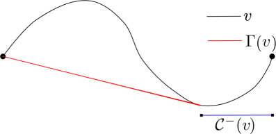
Figure 2.1: Convex envelope and contact set.

An illustration of the convex envelope of a function and its contact set is given in Figure 2.1. From the figure it is intuitively clear that, for fixed values of $v$ on the boundary, how deep the graph of $v$ can go depends only on the values of $v$ at ${\mathcal{C}}^{-}(v)$. The formalization of this observation is the so-called Alexandrov estimate.

Theorem 2.80 (Alexandrov estimate).

Let $v\in C(\bar{B}_{r})$ with $v\geq 0$ on $\partial B_{r}$. If $\Gamma(v)\in C^{1,1}(B_{r})$, then

$$\sup_{B_{r}}v^{-}\leq Cr|\partial\Gamma(v)({\mathcal{C}}^{-}(v))|^{1/d}.$$

In other words, there is a set $A\subset B_{r}$ that satisfies $|B_{r}\setminus A|=0$ and for which we have

$$\sup_{B_{r}}v^{-}\leq Cr\left(\int_{A\cap{\mathcal{C}}^{-}(v)}\det D^{2}\Gamma(v)\right)^{1/d},$$

where the constant $C$ depends only on $d$.

Proof.

Let us, for the sake of completeness, sketch the proof for $v\in C^{2}(B_{r})$, since in this case $\partial\Gamma(v)$ is single valued on ${\mathcal{C}}^{-}(v)$.

Let $M=\sup_{B_{r}}v^{-}/2r$ and assume that $B_{M}\subset\partial\Gamma(v)({\mathcal{C}}^{-}(v))$. If that is the case,

$$M^{d}\leq C|\partial\Gamma(v)({\mathcal{C}}^{-}(v))|,$$

for a constant that depends only on the dimension $d$. This shows the first estimate. On the other hand, a simple change of variables yields

$$|\partial\Gamma(v)({\mathcal{C}}^{-}(v))|=\int_{\partial\Gamma(v)({\mathcal{C}}^{-}(v))}=\int_{{\mathcal{C}}^{-}(v)}\det D^{2}\Gamma(v),$$

so that the second statement follows from the first one.

We now show the inclusion $B_{M}\subset\partial\Gamma(v)({\mathcal{C}}^{-}(v))$. Let $z\in B_{r}$ be a point where $\sup_{B_{r}}v^{-}$ is attained. For ${\bf a}\in B_{M}$, define the affine function

$$L(x)=-\sup_{B_{r}}v^{-}+{\bf a}\cdot(x-z)$$

and notice that $L(z)=-\sup_{B_{r}}v^{-}$ and, for all $x\in B_{r}$,

$$L(x)\leq-\sup_{B_{r}}v^{-}+|{\bf a}||x-z|<-\sup_{B_{r}}v^{-}+2Mr=0.$$

Since $Dv(z)=0$ there is a $x_{1}\in B_{r}$ such that $v(x_{1})<L(x_{1})<0$. In addition, we have that $v(x)\geq 0>L(x)$ for $x\in\partial B_{r}$. This shows that, if $\bar{x}\in B_{r}$ is a point where $v-L$ attains its minimum, then $v(\bar{x})<L(\bar{x})\leq 0$ and $Dv(\bar{x})=DL(\bar{x})={\bf a}$.

Define $\tilde{L}(x)=L(x)+v(\bar{x})-L(\bar{x})$ and notice that $v(\bar{x})=\tilde{L}(\bar{x})$, $Dv(\bar{x})=D\tilde{L}(\bar{x})={\bf a}$ and, for every $x\in B_{r}$ $v(x)\geq\tilde{L}(x)$. In other words, $\tilde{L}$ is a supporting hyperplane for $v$. This shows that $\bar{x}\in{\mathcal{C}}^{-}(v)$ and that ${\bf a}\in\partial\Gamma(v)(\bar{x})$, i.e., $B_{M}\subset\partial\Gamma(v)({\mathcal{C}}^{-}(v))$. ∎

Notice that in Theorem 2.80 only the contact set is relevant. This is due to the fact that if for $x_{0}\in B_{r}$ we have $\Gamma(v)(x_{0})<v(x_{0})$, then locally $\Gamma(v)$ is affine, and thus $D^{2}\Gamma(v)=0$.

With this estimate at hand we can proceed to obtain the fundamental a priori estimate for viscosity solutions, the so-called Alexandrov-Bakelman-Pucci estimate. We begin by providing some motivation for this result. To do so, assume that $u\in C^{2}(\bar{\Omega})$ with $u\geq 0$ on $\partial B_{r}$ satisfies ${\mathcal{L}}u\leq f$ in $B_{r}$. In this setting we have that, for $x\in{\mathcal{C}}^{-}(u)$, $D^{2}u(x)\geq 0$ and, consequently, $A(x):D^{2}u(x)\geq 0$ as well. This, in particular implies that $f(x)\geq 0$. Denote $D=\inf_{x\in\bar{B}_{r}}\det A(x)>0$ and observe that

$$\det A(x)D^{2}u(x)=\det A(x)\det D^{2}u(x)\geq D\det D^{2}u(x)\geq 0.$$

Let $\sigma(A(x)D^{2}u(x))=\{\mu_{i}(x)\}_{i=1}^{d}$, an application of the arithmetic-geometric inequality reveals that

$$\det A(x)D^{2}u(x) =\prod_{i=1}^{d}\mu_{i}(x)=\left(\prod_{i=1}^{d}\mu_{i}(x)^{1/d}\right)^{d}\leq\left(\frac{1}{d}\sum_{i=1}^{d}\mu_{i}(x)\right)^{d}$$

$$=\left(\frac{1}{d}\operatorname*{tr}A(x)D^{2}u(x)\right)^{d}=\left(\frac{1}{d}A(x):D^{2}u(x)\right)^{d}\leq\left(\frac{1}{d}f(x)\right)^{d},$$

where in the last step we used that ${\mathcal{L}}u\leq f$. Theorem 2.80 then yields that

$$\sup_{B_{r}}u^{-}\leq Cr\left(\int_{{\mathcal{C}}^{-}(u)}(f^{+})^{d}\right)^{1/d},$$

for a constant that depends only on $d$ and $D$.

While the considerations presented assumed that we were working with a linear equation, we essentially used that the matrix was uniformly positive definite and bounded, i.e., that the operator ${\mathcal{L}}$ is elliptic. A similar conclusion can be drawn from the fact that an operator is elliptic in the sense of Definition 2.15. We begin by observing [22, Lemma 2.2] that $F$ is uniformly elliptic if and only if

$$F(x,r,{\bf p},M+N)-F(x,r,{\bf p},M)\leq\Lambda|N^{+}|-\lambda|N^{-}|,$$

where $N=N^{+}-N^{-}$ with $N^{+},N^{-}\geq 0$ and $N^{+}N^{-}=0$. Now, if $u$ is a sufficiently smooth subsolution of (2.61), from the observation above we have

$$\leq\Lambda\sum_{\lambda_{i}(u)>0}\lambda_{i}(u)+\lambda\sum_{\lambda_{i}(u)<0}\lambda_{i}(u),$$

where $\sigma(D^{2}u(x))=\{\lambda_{i}(u)\}_{i=1}^{d}$. Similarly, for a supersolution we have

$$f(x)\geq\Lambda\sum_{\lambda_{i}(u)<0}\lambda_{i}(u)+\lambda\sum_{\lambda_{i}(u)>0}\lambda_{i}(u).$$

This motivates the following definitions which, in a sense, describe the class of all possible viscosity solutions to uniformly elliptic equations.

Definition 2.81 (class ${\mathcal{S}}$).

Let the operator $F$ be uniformly elliptic in the sense of Definition 2.15 and denote $f=-F(\cdot,0,\bm{0},0)$. We say that $u\in\underline{{\mathcal{S}}}(\lambda,\Lambda,f)$ if $u\in C(\Omega)$ and the inequality

$$f(x)\leq\Lambda\sum_{\lambda_{i}(u)>0}\lambda_{i}(u)+\lambda\sum_{\lambda_{i}(u)<0}\lambda_{i}(u),$$

holds in the viscosity sense. Similarly, we say that $u\in\overline{{\mathcal{S}}}(\lambda,\Lambda,f)$ if $u\in C(\Omega)$ and

$$f(x)\geq\Lambda\sum_{\lambda_{i}(u)<0}\lambda_{i}(u)+\lambda\sum_{\lambda_{i}(u)>0}\lambda_{i}(u)$$

in the viscosity sense. Finally ${\mathcal{S}}(\lambda,\Lambda,f)=\underline{{\mathcal{S}}}(\lambda,\Lambda,f)\cap\overline{{\mathcal{S}}}(\lambda,\Lambda,f)$.

With this notation at hand we present the Alexandrov-Bakelman-Pucci (ABP) estimate

Theorem 2.82 (ABP estimate).

Let $u\in\overline{{\mathcal{S}}}(\lambda,\Lambda,f)$ in $\Omega$ with $u\geq 0$ on $\partial\Omega$ and assume that $f$ is continuous and bounded in $\Omega$. Then

$$\sup_{\Omega}u^{-}\leq Cr\left(\int_{{\mathcal{C}}^{-}(u)}(f^{+})^{d}\right)^{1/d},$$

where the constant $C$ depends only on $d$, $\lambda$ and $\Lambda$ and $r$ is such that $\Omega\subset B_{r/2}$ and we have extended $u$ by zero outside $\Omega$.

Notice that, as in the Alexandrov estimate, only the contact set ${\mathcal{C}}^{-}(u)$ is relevant in this estimate. Note also that we obtain control of the $L^{\infty}$-norm of $u$ in terms of the $L^{d}$-norm of the data $f$. While Theorem 2.82 is a sort of stability estimate, it is also useful in establishing regularity of solutions. To do so, we begin with the Harnack inequality of Krylov and Safonov; see [117]. In what follows, by $Q_{l}$ we denote a cube with sides parallel to the coordinate axes and of length $l$.

Theorem 2.83 (Harnack inequality).

Let $u\in{\mathcal{S}}(\lambda,\Lambda,f)$ in $Q_{1}$ with $f\in C(Q_{1})\cap L^{\infty}(Q_{1})$. If $u\geq 0$ in $Q_{1}$, then

$$\sup_{Q_{1/2}}u\leq C\left(\inf_{Q_{1}}u+\|f\|_{L^{d}(Q_{1})}\right),$$

where the constant $C$ depends only on $d$, $\lambda$ and $\Lambda$.

Since this will be useful in the sequel, let us now show how from a Harnack inequality one can obtain interior Hölder continuity of functions in ${\mathcal{S}}(\lambda,\Lambda,f)$. We begin with a technical result, commonly referred as an iteration lemma; see [63, Lemma 3.4] and [58, Lemma 8.23].

Lemma 2.84 (iteration).

Let $\varphi:(0,R]\to\mathbb{R}$ be nondecreasing. Assume that for some $A>0$, $B\geq 0$ and $\alpha>\beta$ we have

$$\varphi(\rho)\leq A\left[\left(\frac{\rho}{r}\right)^{\alpha}+\varepsilon\right]\varphi(r)+Br^{\beta}$$

whenever $0<\rho\leq r\leq R$. Then, for every $\gamma\in(\beta,\alpha)$ there is $\varepsilon_{0}$ such that if $\varepsilon<\varepsilon_{0}$, then

$$\varphi(r)\leq C\left[\frac{\varphi(R_{0})}{R_{0}}r^{\gamma}+Br^{\beta}\right],\quad\forall r\in[0,R_{0}),$$

for some fixed constant $C$.

With this result at hand we obtain local Hölder contiuity.

Theorem 2.85 (local Hölder regularity).

Let $u\in{\mathcal{S}}(\lambda,\Lambda,f)$ in $Q_{1}$. then there is $\alpha\in(0,1)$ for which $u\in C^{\alpha}(\bar{Q}_{1/2})$ and

$$\|u\|_{C^{\alpha}(\bar{Q}_{1/2})}\leq C\left(\|u\|_{L^{\infty}(Q_{1})}+\|f\|_{L^{d}(Q_{1})}\right),$$

where the constant $C$ is independent of $u$ and $f$.

Proof.

The proof is rather standard, so we merely sketch it. Let $m_{r}=\inf_{Q_{r}}u$, $M_{r}=\sup_{Q_{r}}u$ and $\varpi_{r}=M_{r}-m_{r}$. Applying the Harnack inequality of Theorem 2.83 to the nonnegative function $u-m_{1}$ yields

$$M_{1/2}-m_{1}\leq C(m_{1/2}-m_{1}+\|f\|_{L^{d}(Q_{1})}).$$

Since the function $M_{1}-u\geq 0$ we can, once more, apply the Harnack inequality to obtain

$$M_{1}-m_{1/2}\leq C(M_{1}-M_{1/2}+\|f\|_{L^{d}(Q_{1})}).$$

Adding these two inequalities yields,

$$\varpi_{1/2}\leq\mu\varpi_{1}+2\|f\|_{L^{d}(Q_{1})},$$

where $\mu=(C-1)/(C+1)\in(0,1)$.

A similar argument for the functions $u_{r}(y)=u(ry)/r^{2}$ and $f_{r}(y)=f(ry)$ with $y\in Q_{1}$ reveals that

$$\varpi_{r}\leq\mu\varpi_{r/2}+2r\|f\|_{L^{d}(Q_{1})}.$$

An application of the iteration Lemma 2.84 with $\varphi(r)=\varpi_{r}$ immediately yields the Hölder continuity and the estimate. ∎

In a similar fashion, we can establish smoothness up to the boundary; see [22, Proposition 4.14].

Theorem 2.86 (global regularity).

Let $\Omega$ be sufficiently smooth and $u\in{\mathcal{S}}(\lambda,\Lambda,f)\cap C(\bar{\Omega})$ with $f\in C(\Omega)$. Let $g=u_{|\partial\Omega}$ and $\varrho$ be a modulus of continuity of $g$. Then there is a modulus of continuity $\varrho^{*}$ of $u$ in $\bar{\Omega}$ which depends only on $\lambda,\Lambda,\varrho,\|f\|_{L^{d}(\Omega)}$ and $\|g\|_{L^{\infty}(\Omega)}$.

We now focus on Hölder estimates for first and second derivatives. To simplify the presentation, in problem (2.20), the PDE takes the form

$$F(x,D^{2}u)=f,\ \text{in }\Omega.$$ (2.87)

To quantify the smoothness of $F$ with respect to the $x$ variable we introduce the function

$$\beta(x)=\sup_{M\in{\mathbb{S}}^{d}}\frac{|F(M,x)-F(M,0)|}{|M|+1}.$$

The local regularity is as follows.

Theorem 2.88 (local $C^{2,\alpha}$ regularity).

Assume that $F$ is uniformly elliptic in the sense of Definition 2.15, $\beta,f\in C^{\alpha}(B_{1})$ and that there is a constant $\bar{\alpha}\in(0,1)$ such that for any $M\in{\mathbb{S}}^{d}$ with $F(0,M)=0$ and $w_{0}\in C(\partial B_{1})$ there is $w\in C^{2}(B_{1})\cap C(\bar{B}_{1})\cap C^{2,\bar{\alpha}}(B_{1/2})$ which satisfies

$$F(0,D^{2}w+M)=0,\ \text{in }B_{1},\quad w=w_{0},\ \text{on }\partial B_{1},$$ (2.89)

with an a priori estimate. If $u$ is a viscosity solution of (2.87) then $u\in C^{2,\alpha}(\bar{B}_{1/2})$ for some $\alpha\in(0,1)$ with an a priori estimate.

To apply this theorem, one must verify that solutions to (2.89) have $C^{2,\bar{\alpha}}$ estimates. For an $F$ that is convex, the Evans-Krylov theorem [23] provides such an estimate.

Theorem 2.90 (Evans-Krylov).

Let $F$ be convex and depend only on $M$. If $u$ is a viscosity solution of $F(D^{2}u)=0$ in $B_{1}$, then

$$\|u\|_{C^{2,\bar{\alpha}}(\bar{B}_{1/2})}\leq C\left(\|u\|_{L^{\infty}(B_{1})}+|F(0)|\right),$$

for some constants $\bar{\alpha}\in(0,1)$ and $C$ that depend only on the dimension $d$ and the ellipticity of $F$.

We mention that Theorem 2.88 can be applied to the Hamilton-Jacobi-Bellman operators of Example 2.17. With the aid of the so-called method of continuity, this allows us to show that solutions to the Dirichlet problem (2.20) for this class of operators are classical.

On the other hand, it is natural to ask if the convexity of $F$ is essential for this result. To understand this, we begin by providing a $C^{1,\alpha}$ estimate without convexity assumptions.

Theorem 2.91 ($C^{1,\alpha}$ regularity).

Let $u$ be a viscosity solution of

$$F(D^{2}u)=0\ \text{in }B_{1}.$$

Then

$$\|u\|_{C^{1,\bar{\alpha}}(\bar{B}_{1/2})}\leq C\left(\|u\|_{L^{\infty}(B_{1})}+|F(0)|\right),$$

where the constants $\bar{\alpha}\in(0,1)$ and $C$ depend only on the dimension and ellipticity of $F$.

A similar argument to Theorem 2.88 allows us to conclude then that, in this setting and under similar assumptions, solutions to (2.20) are locally $C^{1,\alpha}$ with an a priori estimate. However, there exists a series of counterexamples [103, 104, 102] showing that, in general, the convexity assumption on $F$ cannot be removed.

Example 2.92 (nonclassical viscosity solution).

Let $d=5$. Define

$$P_{5}(x)=x_{1}^{3}+\frac{3}{2}x_{1}\left(x_{3}^{2}+x_{4}^{2}-2x_{5}^{2}-2x_{2}^{2}\right)+\frac{3\sqrt{3}}{2}\left(x_{2}x_{3}^{2}-x_{2}x_{4}^{2}+2x_{3}x_{4}x_{5}\right),$$

and, for $\delta\in[0,1)$, $w(x)=P_{5}(x)/|x|^{1+\delta}\in C^{1,1-\delta}(\bar{B}_{1})\setminus C^{2}(B_{1})$. There exists an Isaacs operator $F$ that depends only on $M$ and is Lipschitz, such that $w$ is a viscosity solution of

$$F(D^{2}w)=0,\ \text{in }B_{1},\quad w=P_{5}\ \text{on }\partial B_{1}.$$

The existence of nonclassical solutions in dimensions $3\leq d<5$ is an open problem.

We conclude by providing global regularity results in the general case; see [26, 24, 131].

Theorem 2.93 (global regularity).

Let $\Omega$ be sufficiently regular and $u$ be a viscosity solution to (2.20) with $F$ of the form (2.87) being Lipschitz and uniformly elliptic. If $f\in C^{0,1}(\Omega)$ and, for some $\gamma\in(0,1]$, $g\in C^{1,\gamma}(\partial\Omega)$, then $u\in C^{1,\alpha}(\Omega)\cap C^{0,1}(\bar{\Omega})$ with

$$\|u\|_{C^{1,\alpha}(\Omega)}\leq C\left(\|f\|_{L^{\infty}(\Omega)}+\|g\|_{C^{1,\gamma}(\partial\Omega)}\right),$$

where $\alpha\in(0,1)$ and $C$ depend only on $d$, $\lambda$, $\Lambda$ and the smoothness of $F$.

3 Monotonicity in numerical methods

In this section we review some basic properties of numerical methods and state sufficient conditions to ensure that discrete approximations converge to the solutions of the underlying PDE. The underlying theme of this section is that as the notion of solution to the PDE becomes weaker, additional conditions of the numerical approximation are required to guarantee convergence. For example, for linear differential equations, the well-known Lax-Richtmyer equivalence theorem shows that any consistent scheme is convergent if and only if it is stable; these results extend to mildly nonlinear problems as well. However, in the fully nonlinear regime, consistency and stability are no longer sufficient in general. Rather, additional monotonicity conditions, which essentially mimic the comparison principles discussed in the previous section, are required.

We note that while the content of this section deals with finite difference and finite element methods, the main ideas extend to other discretization techniques as well.

3.1 Stability, consistency and monotonicity implies convergence

As before, let $\Omega$ be an open subset of $\mathbb{R}^{d}$ with Lipschitz boundary $\partial\Omega$. We consider numerical approximations of elliptic problems of the most general form (2.72), which for convenience we recall below

$$F(x,{u},Du,D^{2}u){=0}\quad\text{in }{\Omega},\qquad B(x,u,Du)=0\quad\text{on }\partial\Omega.$$ (3.1)

Here $F\in C({\Omega}\times\mathbb{R}\times\mathbb{R}^{d}\times\mathbb{S}^{d})$ is locally bounded and elliptic in the sense of Definition 2.15.

We further assume that $B\in C(\Omega\times\mathbb{R}\times\mathbb{R}^{d})$ is nonincreasing in its second argument. For the moment, we consider viscosity solutions that satisfy the boundary conditions only in a viscosity sense; see Definition 2.73. In this case, and to simplify the presentation, we define the operator

$${\text{F}}(x,r,{\bf p},M)=\left\{\begin{array}[]{ll}F(x,r,{\bf p},M)&\text{if }x\in\Omega\\ B(x,r,{\bf p})&\text{if }x\in\partial\Omega.\end{array}\right.$$

so that (3.1) becomes

$${\text{F}}[u]:={\text{F}}(x,u,Du,D^{2}u)=0\qquad\text{in }\bar{\Omega}.$$ (3.2)

Note that, since $B$ is nonincreasing in its second argument and $F$ is elliptic, the operator F is elliptic in the sense of Definition 2.15. We further see that, according to Definition 2.73, $u\in C(\bar{\Omega})$ is a viscosity solution to (3.1) (equivalently, (3.2)) if it is a viscosity solution to

$$F(x,u,Du,D^{2}u)=0\qquad\text{in }\Omega,$$

and

$$\max\{F(x,u,Du,D^{2}u),B(x,u,Du)\}\geq 0\quad\text{on }\partial\Omega,$$

$$\min\{F(x,u,Du,D^{2}u),B(x,u,Du)\}\leq 0\quad\text{on }\partial\Omega$$

in the viscosity sense.

We now consider approximation schemes: Find $u_{h}\in X_{h}$ satisfying

$${\text{F}}_{h}[u_{h}]({z})=0\qquad\text{in }\bar{\Omega}_{h},$$ (3.3)

where ${\text{F}}_{h}$ is a locally bounded operator which we may think as an approximation to F, and $X_{h}$ is some finite dimensional space. The operator is parameterized by $h>0$, which we may view as a discretization parameter, or in some cases, a regularization parameter. The discrete domain $\overline{\Omega}_{h}$ is an approximation to $\overline{\Omega}$ with the property $\lim_{h\to 0^{+}}\bar{\Omega}_{h}=\bar{\Omega}$; namely, for all ${z_{0}}\in\bar{\Omega}$, there exists a sequence $\{{z}_{h}\}_{h>0}\subset\bar{\Omega}_{h}$ such that $\lim_{h\to 0^{+}}{z}_{h}={z}_{0}$.

We now address the well-posedness of (3.3), and the sufficient structure conditions on ${\text{F}}_{h}$ to ensure that the discrete solutions to (3.3) (if they exist) converge. As a first step we state the fundamental notions of consistency and stability.

Definition 3.4 (consistency).

The discrete problem (3.3) is said to be consistent with (3.2) if there exists an operator $I_{h}:{C(\bar{\Omega})}\to X_{h}$ such that $I_{h}$ converges uniformly to the identity operator as $h\to 0^{+}$, and for all sequences $\{{z}_{h}\}_{h>0}$ with ${z}_{h}\in\bar{\Omega}_{h}$ and ${z}_{h}\to{z}_{0}\in\bar{\Omega}$ and $\phi\in C^{2}(\bar{\Omega})$,

$$\lim_{h\to 0^{+}}{\text{F}}_{h}[I_{h}\phi]({z}_{h})={\text{F}}[\phi]({z}_{0}).$$

Remark 3.5 (envelopes).

If the operators are not continuous, then the notion of consistency is changed to

$$\limsup_{h\to 0^{+}}{\text{F}}_{h}[I_{h}\phi]({z}_{h})\leq{\text{F}}^{*}[\phi]({z}_{0}),$$

$$\liminf_{h\to 0^{+}}{\text{F}}_{h}[I_{h}\phi]({z}_{h})\geq{\text{F}}_{*}[\phi]({z}_{0}),$$

where ${\text{F}}^{*}$ (resp., ${\text{F}}_{*}$) denote the upper (resp., lower) semi-continuous envelope of F; see Definition 2.66.

Definition 3.6 (stability).

We say that problem (3.3) is stable if, for all $h>0$, there exists a solution $u_{h}\in X_{h}$ to (3.3), and moreover, if ${w_{h}}\in X_{h}$ satisfies ${\text{F}}_{h}[{w_{h}}]=\epsilon_{h}$, then $\|u_{h}-{w_{h}}\|_{L^{\infty}(\bar{\Omega}_{h})}\leq C\|\epsilon_{h}\|_{L^{\infty}(\bar{\Omega}_{h})}$, with $C>0$ independent of $h$.

The following theorem states the well-known result that, for linear problems with classical solutions, consistent and stable schemes converge.

Theorem 3.7 (Lax-Richtmyer).

Suppose that ${\text{F}}_{h}$ is an affine operator, and that there exists a classical solution $u\in C^{2}(\bar{\Omega})$ satisfying (3.2). Suppose further that problem (3.3) is stable and that the operator in Definition 3.4 satisfies the stronger condition $\lim_{h\to 0^{+}}\|{\text{F}}_{h}[I_{h}u]\|_{L^{\infty}(\bar{\Omega}_{h})}=0$. Then $u_{h}$ converges locally uniformly to $u$.

Proof.

By the given assumptions, there exists a linear operator ${\text{G}}_{h}$ and a function ${\text{l}}_{h}$ such that

$${\text{F}}_{h}[v_{h}]({z})={\text{G}}_{h}[v_{h}]({z})-{\text{l}}_{h}({z})\quad{z}\in\bar{\Omega}_{h}.$$

The stability of the scheme shows that ${\text{G}}_{h}[\cdot]$ is an isomorphism whose inverse is bounded independent of $h$. Since

$${\text{G}}_{h}[u_{h}-I_{h}u]={\text{l}}_{h}-{\text{G}}_{h}[I_{h}u]=-{\text{F}}_{h}[I_{h}u],$$

the consistency of the scheme implies that $\lim_{h\to 0^{+}}\|u_{h}-I_{h}u\|_{L^{\infty}(\bar{\Omega}_{h})}=0$, and thus, since $I_{h}$ converges to the identity operator, $u_{h}$ converges locally uniformly to $u$. ∎

While Theorem 3.7 is a useful result for a large class of problems, it is not applicable to fully nonlinear problems nor to weaker notions of solutions, in particular, viscosity solutions. The issue is that, if $u$ is not a classical solution, then the approximation $I_{h}u$ may not be well–defined, and the consistency ${\text{F}}_{h}[I_{h}u]\to 0$ used in the proof of Theorem 3.7 is no longer valid. Rather, to prove convergence to viscosity solutions, an additional structure condition is required. This requirement is summarized in the following definition.

Definition 3.8 (monotone operator).

The discrete operator ${\text{F}}_{h}$ is said to be monotone if whenever $u_{h}-v_{h}$ has a global nonnegative maximum at ${z}\in\bar{\Omega}_{h}$ we have

$${\text{F}}_{h}[u_{h}]({z})\leq{\text{F}}_{h}[v_{h}]({z}).$$ (3.9)

Remark 3.10 (monotonicity).

The notion of monotonicity is essentially a discrete version of ellipticity. Indeed, following the proof of Theorem 2.22, if F is an elliptic operator in the sense of Definition 2.15, and if $u-v$, with $u,v\in C^{2}(\bar{\Omega})$, has a global nonnegative maximum at $x\in\bar{\Omega}$, then $u(x)\geq v(x)$, $Du(x)=Dv(x)$ and $D^{2}u(x)\leq D^{2}v(x)$. Since F is nonincreasing in its second argument, and nondecreasing in its fourth, we have

$${\text{F}}[u](x)={\text{F}}(x,u(x),Du(x),D^{2}u(x))\leq{\text{F}}(x,v(x),Dv(x),D^{2}v(x))={\text{F}}[v](x).$$

Conversely, it can be shown that the operator F is elliptic if, whenever $u-v$ has a global nonnegative maximum at $x\in\bar{\Omega}$, then ${\text{F}}[u](x)\leq{\text{F}}[v](x)$.

Consistency, stability and monotonicity are the three sufficient ingredients to guarantee convergence to viscosity solutions. The following result closely follows [8, Theorem 2.1].

Theorem 3.11 (Barles-Souganidis).

Suppose that problem (3.3) is consistent, stable and monotone in the sense of Definitions 3.4, 3.6, and 3.8, respectively. Suppose further that F satisfies the comparison principle given in Definition 2.68. Then $u_{h}$ converges locally uniformly to the unique continuous viscosity solution of (3.2).

Proof.

Define $\bar{u}\in USC(\Omega)$ and $\underline{u}\in LSC(\Omega)$ by

$$\bar{u}(x):=\mathop{\limsup_{y\to x}}_{h\to 0^{+}}u_{h}(y),\quad\underline{u}(x):=\mathop{\liminf_{y\to x}}_{h\to 0^{+}}u_{h}(y),\quad x\in\bar{\Omega}.$$ (3.12)

Note that the stability of the scheme implies that both $\bar{u}$ and $\underline{u}$ are well-defined. The proof proceeds by showing that $\bar{u}$ and $\underline{u}$ are (viscosity) subsolutions and supersolutions to (3.2), respectively, and then appealing to the comparison principle.

To this end, suppose that $z_{0}\in{\Omega}$ is a strict local maximum of $\underline{u}-\phi$ for some $\phi\in C^{2}({\Omega})$. Then standard arguments show that there exists sequences $\{h_{n}\}_{n=1}^{\infty}$ and $\{z_{h_{n}}\}_{n=1}^{\infty}$ such that

$$z_{n}\to 0,\quad z_{h_{n}}\to x_{0},\quad\text{ as }n\to\infty,$$

and $u_{h_{n}}-I_{h_{n}}\phi$ obtains a strict local maximum at $z_{h_{n}}$. Since ${\text{F}}_{h_{n}}[u_{h_{n}}](z_{h_{n}})=0$, the monotonicity of the discrete operator implies that

$${\text{F}}_{h_{n}}[I_{h_{n}}\phi](z_{h_{n}})\geq 0.$$

Passing to the limit, together with consistency of the scheme, yields

$$0 \leq\lim_{n\to\infty}{\text{F}}_{h_{n}}[I_{h_{n}}\phi](z_{h_{n}})={\text{F}}[\phi](z_{0}).$$

Similar arguments show that if $\bar{u}-\phi$ obtains a strict minimum at $z_{0}\in{\Omega}$, there holds $0\geq{\text{F}}[\phi](z_{0})$. Thus, $\bar{u}$ and $\underline{u}$ are subsolutions and supersolutions to (3.2), respectively. Since $\underline{u}\leq\bar{u}$, the comparison principle of F implies that $\underline{u}=\bar{u}=u$, and $u$ is the viscosity solution to (3.2). ∎

We once again mention that the problems and discretizations considered so far take into account the boundary conditions in a viscosity sense. While this setup simplifies the proof of convergence, it may have practical limitations since the framework requires a consistent and monotone discretization of both the boundary conditions and the differential operator for all $x\in\partial\Omega$ and smooth functions $\phi$. Also recall that, in general, viscosity boundary conditions are not equivalent to those imposed pointwise unless other conditions are assumed; see Proposition 2.75. Here we turn our attention to the elliptic boundary value problem (2.20), where the Dirichlet boundary condition is understood in the classical sense; see Definition 2.67.

To this end, we consider approximations of the form:

$$F_{h}[u_{h}]=0\quad\text{in }\Omega^{I}_{h},\qquad u_{h}=g_{h}\quad\text{on }\Omega_{h}^{B},$$ (3.13)

where $g_{h}=I_{h}g\in X_{h}$ is a discrete approximation to the Dirichlet data $g\in C(\bar{\Omega})$, $\Omega^{I}_{h}$ and $\Omega^{B}_{h}$ are disjoint sets with $\Omega_{h}^{I}\to\Omega$ and $\Omega_{h}^{B}\to\partial\Omega$ as $h\to 0^{+}$. Note that, with minor notational changes, the notions of consistency, stability, and monotonicity are applicable to the operator $F_{h}$. A natural question then, is whether the results of Theorem 3.11 carry over to the discrete problem (3.13). This issue is addressed in the next theorem.

Theorem 3.14 (convergence).

Suppose that $F_{h}$ is a consistent, stable, and monotone operator. Suppose further that either

1. $\underline{u}(x)\geq g(x)$ and $\bar{u}(x)\leq g(x)$ for all $x\in\partial\Omega$, where $\underline{u},\bar{u}$ are given by (3.12); or

2. The sequence of solutions $\{u_{h}\}_{h>0}$ is equicontinuous.

Then $u_{h}$ converges locally uniformly to the unique continuous viscosity solution of (3.1) with $B(x,u,Du)={g-u}$.

Proof.

The proof of the first case (i) follows directly from the arguments given in Theorem 3.11. The proof of the second case (ii) follows from the Arzelà-Ascoli theorem, and again appealing to the proof of Theorem 3.11. ∎

3.2 Monotonicity in finite difference schemes

Here we discuss basic monotonicity results of finite difference schemes. The main message given in this section is that for any uniformly elliptic operator, one can construct a consistent and monotone finite difference scheme. The drawback however is that monotonicity requires a wide-stencil, which may severely impact its practical use. Much of the material in this section is found in [88, 89, 76, 101, 113].

For simplicity we assume that the domain $\Omega$ is discretized on an equally spaced cartesian grid and that each coordinate direction is discretized uniformly; in particular, by a possible change of coordinates, we assume that the grid is given by

$$\bar{\Omega}_{h}=\mathbb{Z}^{d}_{h}\cap\overline{\Omega},\quad\text{with }\mathbb{Z}_{h}^{d}:=\{he:\ e\in\mathbb{Z}^{d}\},$$

where $h>0$ is the grid scale and $\mathbb{Z}^{d}$ is the set of $d$–tuples of integers. A finite subset $S\subset\mathbb{Z}^{d}\backslash\{0\}$ is called a stencil, and the space of nodal functions, denoted by $X_{h}^{fd}$, consist of real-valued functions with domain $\bar{\Omega}_{h}$. The canonical interpolant $I_{h}^{fd}:C^{0}(\bar{\Omega})\to{X_{h}^{fd}}$ is the operator satisfying $I_{h}^{fd}v({z})=v({z})$ for all ${z}\in\bar{\Omega}_{h}$. We assume the existence of a positive integer $m$ such that $S$ is of the form

$$S=\{y:\ y\in\mathbb{Z}^{d}\backslash\{0\}:\ |y|_{\ell^{\infty}}\leq m\}.$$ (3.15)

The value $m$ satisfying (3.15) is called the stencil size of $S$. The cardinality of $S$ is $|S|:=(2m+1)^{d}-1$.

We consider finite difference schemes with stencil $S$ acting on grid functions. These discrete operators are thus of the (implicit) form

$$F_{h}[v_{h}]({z})=F_{h}({z},v_{h}(z),Tv_{h}({z})),$$ (3.16)

where $Tv_{h}(x)=\{v_{h}(x+hy):\ y\in S\}$ is the set of translates of $v_{h}(x)$ with respect to the stencil. The method (3.16) is called a one-step scheme if $m=1$, i.e., the value $F_{h}[v_{h}]({z})$ only depends on $z$, $v_{h}({z})$, and the values of $v_{h}$ at neighboring points of ${z}$. Otherwise, we call the scheme a wide-stencil scheme if $m\geq 2$.

To construct monotone schemes, we first reformulate this property so that it is easier to work with.

Definition 3.17 (nonegative operator).

The operator $F_{h}$ is of nonnegative type (or simply, nonnegative) if

$$F_{h}({z},{r},q+\tau)\geq F_{h}({z},{r},q)\geq F_{h}({z},{r}+t,q+\tau)$$ (3.18)

for all ${z}\in\mathbb{R}^{d}$, ${r},t\in\mathbb{R}$, and $q,\tau\in\mathbb{R}^{|S|}$ satisfying

$$0\leq\tau_{i}\leq t\qquad i=1,2,\ldots|S|.$$ (3.19)

We see that if $F_{h}$ is of nonnegative type then $F_{h}$ is nonincreasing in its second argument and nondecreasing in its third argument. If $F_{h}$ is differentiable, then it is of nonnegative type provided that

$$\frac{\partial F_{h}}{\partial q_{i}}\geq 0\ (i=1,2,\ldots,|S|),\qquad\frac{\partial F_{h}}{\partial{r}}+\sum_{i=1}^{|S|}\frac{\partial F_{h}}{\partial q_{i}}\leq 0.$$

Remark 3.20 (reformulation).

Alternatively, as in [113], one can consider finite difference schemes of the form

$$F_{h}[u]({z})=G_{h}({z},u({z}),u({z})-Tu({z})).$$

Using the correspondence $F_{h}({z},{r},q)=G_{h}({z},{r},{r}{\bm{1}}-q)$, one sees that $F_{h}$ is of nonnegative type if and only if $G_{h}$ is nonincreasing in its second and third arguments.

Let us now show that nonegativity is nothing but a reformulation of monotonicity.

Lemma 3.21 (equivalence).

A finite difference scheme of the form (3.16) is monotone if and only if it is of nonnegative type.

Proof.

Suppose that $F_{h}$ is of nonnegative type. Let $u_{h}$ and $v_{h}$ be two grid functions such that $u_{h}-v_{h}$ has a global nonnegative maximum at some grid point ${z}$. Set ${r}=v_{h}({z})$, $t=u_{h}({z})-v_{h}({z})\geq 0$, $q_{i}=v_{h}({z}+hy_{i})$, and $\tau_{i}=\max\{0,u_{h}({z}+hy_{i})-v_{h}({z}+hy_{i})\}$, so that $t\geq\tau_{i}$. Noting that $q_{i}+\tau_{i}=v_{h}({z}+hy_{i})+\max\{0,u_{h}({z}+hy_{i})-v_{h}({z}+hy_{i})\}\geq u_{h}({z}+hy_{i})$, and $F_{h}$ is non–decreasing in its third argument, we find that $F_{h}[u_{h}]({z})\leq F_{h}({z},{r}+t,q+\tau).$ Therefore by the second inequality in (3.18) we have

$$F_{h}[u_{h}]({z})\leq F_{h}({z},{r}+t,q+\tau)\leq F_{h}({z},{r},q)=F_{h}[v_{h}]({z}).$$

Thus, $F_{h}$ is monotone.

Now suppose that $F_{h}$ is monotone. Let ${z}\in\mathbb{R}^{d}$ be fixed, and let ${r},t\in\mathbb{R}$ and $q,\tau\in\mathbb{R}^{|S|}$ satisfy (3.18). Then define the grid functions $u_{h},v_{h}$ (locally) as

$$v_{h}({z})={r},\quad v_{h}({z}+hy_{i})=q_{i},\quad u_{h}({z})={r}+t,\quad u_{h}({z}+y_{i})=q_{i}+\tau_{i}.$$

Then

$$u_{h}({z})-v_{h}({z})=t\geq\tau_{i}=u_{h}({z}+hy_{i})-v_{h}({z}+hy_{i}),$$

i.e., $u_{h}-v_{h}$ has a nonnegative maximum at ${z}$. The monotonicity of $F_{h}$ yields $F_{h}[u_{h}]({z})\leq F_{h}[v_{h}]({z})$; thus

$$F_{h}({z},{r}+t,q+\tau)\leq F_{h}({z},{r},q).$$ (3.22)

On the other hand, with $v_{h}$ as before, we consider the grid function $w_{h}$ with

$$w_{h}({z})={r},\quad w_{h}({z}+hy_{i})=q_{i}+\tau_{i}.$$

Then $v_{h}-w_{h}$ has a global maximum at ${z}$ and thus

$$F_{h}({z},{r},q)=F_{h}[v_{h}]({z})\leq F_{h}[w_{h}]({z})=F_{h}({z},{r},q+\tau).$$ (3.23)

We conclude from (3.22)–(3.23) that $F_{h}$ is of nonnegative type. ∎

Following the framework given in [88, 89, 76] we consider discrete operators constructed from the first and second order difference operators

$$\delta_{y,h}^{+}u({z}): =\frac{1}{h}\big{(}u({z}+hy)-u({z})\big{)},$$

$$\delta_{y,h}^{-}u({z}): =\frac{1}{h}\big{(}u({z})-u({z}-hy)\big{)},$$

$$\delta_{y,h}u({z}): =\frac{1}{2}\big{(}\delta_{y}^{+}+\delta_{y}^{-}\big{)}u({z})=\frac{1}{2h}\big{(}u({z}+hy)-u({z}-hy)\big{)},$$

$$\delta_{y,h}^{2}u({z}): =\frac{1}{h^{2}}\big{(}u({z}+hy)-2u(x)+u({z}-hy)\big{)},$$

with $y\in S$. Taylor’s Theorem shows that the differences $\delta_{y,h}^{\pm}u(z)$ are first order approximations to $\frac{\partial u({z})}{\partial y}:=Du({z})\cdot y$, whereas $\delta_{y,h}u({z})$ and $\delta_{y,h}^{2}u({z})$ are second-order approximations to $\frac{\partial u({z})}{\partial y}$ and $\frac{\partial^{2}u({z})}{\partial y^{2}}:=y\cdot D^{2}u({z})y$, respectively; by this, we mean that $|\frac{\partial^{\pm}u({z})}{\partial y}-\delta_{y,h}^{\pm}u({z})|=\mathcal{O}(h|y|^{2})$, $|\frac{\partial u({z})}{\partial y}-\delta_{y,h}u({z})|=\mathcal{O}(h^{2}|y|^{3})$, and $|\frac{\partial^{2}u({z})}{\partial y^{2}}-\delta^{2}_{y,h}u({z})|=\mathcal{O}(h^{2}|y|^{4})$ for sufficiently smooth $u$.

Let $\delta_{h}u_{h}({z})=\{\delta_{y,h}u_{h}({z}):\ y\in S\}$ and $\delta^{2}_{h}u_{h}({z})=\{\delta_{y,h}^{2}u_{h}({z}):\ y\in S\}$. Then a consistent and monotone finite difference scheme can be constructed in the form [88, 89, 101]

$$F_{h}[u_{h}]({z})=\mathcal{F}_{h}({z},u_{h}({z}),\delta_{h}u_{h}({z}),\delta^{2}_{h}u_{h}({z})),$$ (3.24)

where $\mathcal{F}_{h}:\Omega_{h}\times\mathbb{R}\times\mathbb{R}^{|S|}\times\mathbb{R}^{|S|}\to\mathbb{R}$. Denote points in the domain of $\mathcal{F}_{h}$ by $({z},{r},q,s)$ and assume that $\mathcal{F}_{h}$ is symmetric with respect to $\pm q_{\pm i}$ and $s_{\pm i}$. Then from Definition 3.21 and Lemma 3.21, we see that $F_{h}$ of the form (3.24) is monotone provided that

$$\frac{h}{2}\Big{|}\frac{\partial\mathcal{F}}{\partial q_{i}}\Big{|}\leq\frac{\partial\mathcal{F}}{\partial s_{i}}\quad i=1,2,\ldots,|S|,\quad\text{and}\quad\frac{\partial\mathcal{F}}{\partial{r}}\leq 0.$$ (3.25)

In what follows, we require slightly stronger conditions on the operator $\mathcal{F}_{h}$.

Definition 3.26 (positive operator).

An operator of the form (3.24) is of positive type (or simply, positive) if (3.25) is satisfied and there exists $\lambda_{0,h}>0$ and an orthogonal set of vectors $\{y_{i}\}_{i=1}^{d}\subset S$ such that

$$\lambda_{0,h}+\frac{h}{2}\Big{|}\frac{\partial\mathcal{F}}{\partial q_{i}}\Big{|}\leq\frac{\partial\mathcal{F}}{\partial s_{i}}.$$

Remark 3.27 (discrete ellipticity).

The discrete ellipticity constant $\lambda_{0,h}$ may depend on the stencil size $m$; see Theorem 3.67.

3.3 Finite difference stability estimates: Alexandrov estimates and Alexandrov-Bakelman-Pucci maximum principle

We now turn our attention to maximum principles of discrete operators, and correspondingly, stability estimates. As a starting point, we discuss monotone finite difference schemes for the linear nondivergence form PDEs of Example 2.16

$$F[u]=\mathcal{L}u-f=A:D^{2}u-f=0.$$ (3.28)

While this setting may seem overly simplistic, as we shall see, the construction and theoretical results for the linear problem form all of the necessary tools to approximate viscosity solutions of nonlinear elliptic equations.

We assume that $f\in C(\bar{\Omega})$ and that the coefficient matrix $A$ is bounded and uniformly symmetric positive definite. It is then reasonable to assume that $F_{h}$ is linear and thus has the form

$$F_{h}[u_{h}]({z})={\mathcal{L}_{h}u_{h}(z)-f(z)}:=\sum_{y\in S}a_{y}({z})\delta_{y,h}^{2}u_{h}({z})-f({z})$$ (3.29)

for nodal functions (or coefficients) $a_{y}$. Applying Definition 3.17 to (3.29), we see that $F_{h}$ is nonnegative (and hence monotone) provided

$$a_{y}({z})\geq 0,$$ (3.30)

and of positive type if

$$a_{y_{i}}({z})\geq\lambda_{0,h}\qquad i=1,2,\ldots,d.$$

for some orthogonal basis $\{y_{i}\}_{i=1}^{d}\subset S$. These inequalities suggest that the negation of the ensuing system is an $M$–matrix, and hence solutions to the discrete problem satisfy certain maximum principles, analogous to the continuous setting. This issue is discussed in the next section.

3.3.1 Finite difference Alexandrov estimates

In this section we state and prove ABP maximum principles for grid functions. To get started, we first specify the fundamental notion of interior and boundary nodes used in this section.

Definition 3.31 (interior and boundary nodes).

For a discrete operator $F_{h}$, we define the set of interior nodes $\Omega^{I}_{h}$ as the set of grid points ${z}\in\bar{\Omega}_{h}$ such that for any mesh function $v_{h}$, $F_{h}[v_{h}]({z})$ depends only on the translates of $v_{h}$ at points in $\Omega_{h}$. The set of boundary nodes are given by $\Omega_{h}^{B}:=\bar{\Omega}_{h}\backslash\Omega_{h}^{I}$.

Remark 3.32 (discrete domain).

If $F_{h}$ is a one-step method (i.e., $m=1$), then $\Omega_{h}^{B}=\partial\Omega\cap\mathbb{Z}_{h}^{d}$ and $\Omega_{h}^{I}=\Omega\cap\mathbb{Z}_{h}^{d}$.

As a next step we introduce and discuss several basic properties of convexity and the subdifferential for discrete (nodal) functions.

Definition 3.33 (convex nodal function).

We say that a nodal function $v_{h}\in X_{h}^{fd}$ is a convex nodal function if there is a supporting hyperplane of $v_{h}$ at all interior nodes $z\in\Omega_{h}^{I}.$

Note that if $v_{h}$ is the nodal interpolant of a convex function, then $v_{h}$ is a convex nodal functions.

Definition 3.34 (discrete convex envelope).

Let $R>0$ be sufficiently large such that $\bar{\Omega}$ (and hence $\bar{\Omega}_{h}$) is compactly contained in a ball $B_{R}$. For a nodal function (or continuous function) $v_{h}$ with $v_{h}\geq 0$ on $\Omega_{h}^{B}$, we extend $v^{-}_{h}$ to $B_{R,h}\backslash\bar{\Omega}_{h}$ by zero, where $B_{R,h}={B_{R}}\cap\mathbb{Z}_{h}^{d}$. We define the discrete convex envelope of $-v^{-}_{h}$ as

$$\Gamma_{h}(v_{h})(x):=\sup\{L(x):\ L(z)\leq-v^{-}_{h}(z)\ \forall z\in B_{R,h},\ L\in\mathbb{P}_{1}\}$$ (3.35)

for all $x\in\bar{B}_{R}$.

Remark 3.36 (discrete convexity).

There are some subtle issues in the above definitions that require some elaboration.

1. If $v_{h}\in X_{h}^{fd}$ is convex and $v_{h}\leq 0$, then we have

   $$v_{h}(z)=\Gamma_{h}(v_{h})(z)\quad\text{for all $z\in\Omega_{h}^{I}$.}$$ (3.37)

   Thus, $\Gamma_{h}(v_{h})$ is a natural convex extension of $v_{h}$. With an abuse of notation, we still use $v_{h}$ to denote the convex envelope of this nodal function.

2. Since for every $x\in\partial B_{R}$, there exists an affine function $L$ with $L(z)\leq-v_{h}^{-}(z)$ for all $z\in\bar{\Omega}_{h}$ and $L(x)=0$, we conclude that $\Gamma_{h}(v_{h})=0$ on $\partial B_{R}$.

3. Definition 3.34 implies that $\Gamma_{h}(v_{h})$ is a convex, piecewise linear function with respect to a simplicial triangulation. The vertices of the triangulation are a subset of the gridpoints $B_{R,h}$, and its configuration depends on $v_{h}$; see Examples 3.87–3.88.

4. For $v_{h}\in X_{h}^{fd}$, denote by $\tilde{v}_{h}\in C(\bar{\Omega})$ the canonical multi-linear function. Then, since the inequality constraints in (3.35) are only posed on a discrete set of points, and since $\tilde{v}_{h}$ is not necessarily piecewise affine, we have $\Gamma(\tilde{v}_{h})\neq\Gamma_{h}(v_{h})$ in general [28].

Next, we require the notion of a subdifferential acting on nodal functions. Recall from Definition 2.78 that the subdifferential requires function values at all points of the domain $\Omega$, and thus, this notion is not directly applicable to the discrete case. Instead, with a slight abuse of notation, we define its natural extension to nodal functions as follows:

$$\partial v_{h}(z)=\big{\{}{\bf p}\in\mathbb{R}^{d}:\ v_{h}(x)-v_{h}(z)\geq{\bf p}\cdot(x-z),\ \forall x\in\bar{\Omega}_{h}\big{\}}$$ (3.38)

for all $z\in\bar{\Omega}_{h}$ and $v_{h}\in X_{h}^{fd}$.

Lemma 3.39 (discrete subdifferential).

If $v_{h}\in X_{h}^{fd}$ is a convex nodal function, then $\partial v_{h}(z)=\partial\Gamma_{h}(v_{h})(z)$ for all $z\in\Omega_{h}^{I}$.

Proof.

Thanks to (3.37), if ${\bf p}\in\partial\Gamma_{h}(v_{h})(z)$, that is,

$$\Gamma_{h}(v_{h})(x)\geq\Gamma_{h}(v_{h})(z)+{\bf p}\cdot(x-z)\quad\forall x\in\Omega,$$

then ${\bf p}\in\partial v_{h}(z)$.

Conversely, let $\mathcal{T}_{z}$ be a local mesh induced by $\Gamma(u_{h})(z)$, $K\in\mathcal{T}_{z}$ a $d$-dimensional simplex, and $\{z_{j}\}_{j=1}^{d+1}$ be the vertices of $K$. If ${\bf p}\in\partial v_{h}(z)$, then we clearly have $v_{h}(x)\geq v_{h}(z)+{\bf p}\cdot(x-z)$ for all vertices $x\in\bar{\Omega}_{h}$. Again, thanks to (3.37), we have $\Gamma(v_{h})(z_{i})\geq\Gamma(v_{h})(z)+{\bf p}\cdot(z_{i}-z)$ for all vertices. Since $\Gamma(v_{h})$ is linear on element $K$, we have $\Gamma(v_{h})(x)\geq\Gamma(v_{h})(z)+{\bf p}\cdot(x-z)$ for any $x\in K$. This shows that ${\bf p}\in{\partial}\Gamma(u_{h})(z)$ as well. ∎

Let us state two properties of subdifferentials. The proof of the first one follows directly from its definition.

Lemma 3.40 (monotonicity of subdifferential).

Let $w_{h},v_{h}\in X_{h}^{fd}$ be two convex nodal functions such that, for a fixed $z_{*}\in\bar{\Omega}_{h}$, $w_{h}(z_{*})=v_{h}(z_{*})$ and $w_{h}(z)\leq v_{h}(z)$ for all $z\neq z_{*}$. Then,

$$\partial w_{h}(z_{*})\subset\partial v_{h}(z_{*}).$$

Lemma 3.41 (addition inequality).

Let $w_{h}$ and $v_{h}$ be two convex nodal functions. Then

$$\partial w_{h}(z)+\partial v_{h}(z)\subset\partial(w_{h}+v_{h})(z)\quad\forall z\in\Omega_{h}^{I},$$

where $\partial w_{h}(z)+\partial v_{h}(z)$ is the Minkowski sum:

$$\partial w_{h}(z)+\partial v_{h}(z)=\{{\bf p}+{\bf q}\in\mathbb{R}^{d}:{\bf p}\in\partial w_{h}(z),{\bf q}\in\partial v_{h}(z)\}$$

Proof.

We note that if ${\bf p}\in\partial w_{h}(z)$ and ${\bf q}\in\partial v_{h}(z)$, then

$$w_{h}(x)\geq w_{h}(z)+w\cdot(x-z)\quad\text{and}\quad v_{h}(x)\geq v_{h}(z)+v\cdot(x-z)$$

for all $x\in\bar{\Omega}_{h}$. Adding both inequalities yields

$$w_{h}(x)+v_{h}(x)\geq w_{h}(z)+v_{h}(z)+({\bf p}+{\bf q})\cdot(x-z)$$

which implies that $({\bf p}+{\bf q})\in\partial(w_{h}+v_{h})$. ∎

Given a convex nodal function $u_{h}$, computing its discrete subdifferetial set is not a trivial task. The following lemma shows that it involves computing the convex envelope of $u_{h}$.

Lemma 3.42 (characterization of subdifferential).

Let $u_{h}$ be a convex nodal function, and let ${\mathcal{T}_{h}}$ be the simplicial mesh induced by its convex envelope. The subdifferential of $u_{h}$ at $z$ is the convex hull of the piecewise gradient, that is,

$${\operatorname{conv}\left\{Du_{h}|_{K},K\in{\mathcal{T}_{h}},\ z\in{\bar{K}}\right\}}.$$

Here, $Du_{h}$ is the gradient of the piecewise linear polynomial induced by $u_{h}$ and $\mathcal{T}_{h}$.

As final preparation to state the finite difference version of the Alexandrov estimate, we define the nodal contact set.

Definition 3.43 (nodal contact set).

Let $v_{h}$ be either a nodal function or a continuous function with $v_{h}\geq 0$ on $\Omega_{h}^{B}$. The (lower) nodal contact set of $v_{h}$ is given by

$$\mathcal{C}_{h}^{-}(v_{h})=\{z\in\Omega_{h}^{I}:\ \Gamma_{h}(v_{h})(z)=v_{h}(z)\}.$$

Note that, for $x\in\mathcal{C}_{h}^{-}(v_{h})$, we have

$$v_{h}(z)\geq\Gamma_{h}(v_{h})(z)\geq v_{h}(x)+{\bf p}\cdot(z-x)\quad\forall z\in B_{R,h},\ \forall{\bf p}\in\partial\Gamma_{h}(v_{h})(x).$$

We are now ready to state and prove the finite difference Alexandrov estimate. Recall that we assume $\Omega$ is compactly contained in a ball $B_{R}$ of radius $R$, and that we set $B_{R,h}=B_{R}\cap\mathbb{Z}_{h}^{d}$.

Lemma 3.44 (finite difference Alexandrov estimate).

Let $v_{h}\in X_{h}^{fd}$ with $v_{h}\geq 0$ on $\Omega_{h}^{B}$. Then

$$\sup_{\bar{\Omega}_{h}}v_{h}^{-}\leq C{R}\Big{(}\sum_{{z}\in\mathcal{C}_{h}^{-}(v_{h})}|\partial\Gamma_{h}(v_{h})({z})|\Big{)}^{1/d},$$ (3.45)

where the constant $C>0$ depends only on $d$.

Proof.

We follow the arguments given in [109, Proposition 5.1]; also see [88].

Let ${z}_{*}\in B_{R,h}$ satisfy $\sup_{B_{R,h}}v_{h}^{-}=v_{h}^{-}({z}_{*})$, and let $L$ be a horizontal plane touching $v_{h}$ from below at ${z}_{*}$. By Definition 3.34 we have

$$\Gamma_{h}(v_{h})({z})\geq L({z})=L({z}_{*})=v_{h}({z}_{*})\qquad\forall{z}\in B_{R,h}.$$

Thus, $\sup_{B_{R,h}}\Gamma_{h}(v_{h})^{-}\leq v_{h}^{-}({z}_{*})$. Since $\Gamma_{h}(v_{h})\leq v_{h}$ on $B_{R,h}$ implies

$$\sup_{B_{R,h}}v_{h}^{-}\leq\sup_{B_{R,h}}\Gamma_{h}(v_{h})^{-},$$

we conclude that

$$\sup_{\bar{\Omega}_{h}}v_{h}^{-}=\sup_{B_{R,h}}v_{h}^{-}=\sup_{B_{R,h}}\Gamma_{h}(v_{h})^{-}=\sup_{B_{R}}\Gamma_{h}(v_{h})^{-}.$$

Therefore to conclude the proof, it suffices to show that

$$\max_{\bar{\Omega}_{h}}\Gamma_{h}(v_{h})^{-}\leq C{R}\Big{(}\sum_{{z}\in\mathcal{C}_{h}^{-}(v_{h})}|\partial\Gamma_{h}(v_{h})({z})|\Big{)}^{1/d}.$$

This is done in three steps.

Step 1. Let $K(x)$ be the cone with vertex ${z}_{*}$ satisfying

$$K({z}_{*})=-\sup_{B_{R}}\Gamma_{h}(v_{h})^{-}=:-M\quad\text{ and }\quad K(x)=0\text{ on $\partial B_{R}$},$$

and assume that $M>0$ for otherwise (3.45) is trivial. We note that for any vector ${\bf p}\in B_{\frac{M}{2R}}(0)$, the affine function $L(x)=-M+{\bf p}\cdot{x-{z}_{*}}$ is a supporting plane of $K(x)$ at point ${z}_{*}$, namely $L(x)\leq K(x)$ for all $x\in B_{R}$ and $L({z}_{*})=K({z}_{*})$. This implies that $\partial K({z}_{*})\supset B_{\frac{M}{2R}}(0),$ and therefore

$$|\partial K({z}_{*})|\geq C\left(\frac{M}{R}\right)^{d}.$$

Step 2. We claim that

$$\partial K({z}_{*})\subset\bigcup_{{z}\in\mathcal{C}^{-}_{h}(v_{h})}\partial\Gamma_{h}(v_{h})({z}).$$ (3.46)

This is equivalent to showing that for any supporting plane $L$ of $K$ at ${z}_{*}$, there is a parallel supporting plane $\tilde{L}$ for $\Gamma_{h}(v_{h})$ at some contact node $y\in\mathcal{C}_{h}^{-}(v_{h})$.

Consider the (nodal) function $v_{h}-L$, and observe that $v_{h}\geq 0$ on $\Omega_{h}^{B}$ and $v_{h}({z}_{*})=K({z}_{*})=L({z}_{*})$, whence

$$v_{h}({z})-L({z}) \;\geq\;K({z})-L({z})\geq 0\qquad\text{on $\Omega_{h}^{B}$},$$

$$v_{h}({z}_{*})-L({z}_{*}) \;=\;K({z}_{*})-L({z}_{*})=0.$$

We infer that $v_{h}-L$ attains a non-positive minimum for some $x\in\Omega_{h}^{I}$. Hence, $\widetilde{L}({z})=L({z})+v_{h}(x)-L(x)$ satisfies $\tilde{L}({z})\leq v_{h}({z})$ for all ${z\in}B_{R,h}$ and $\tilde{L}(x)=v_{h}(x)$. Applying Definition 3.34 we conclude that $\tilde{L}\leq\Gamma_{h}(v_{h})\leq v_{h}$ and therefore $\Gamma_{h}(v_{h})(x)=v_{h}(x)$; thus $x\in\mathcal{C}_{h}^{-}(v_{h})$.

Step 3. Computing Lebesgue measures in (3.46) yields

$$C\left(\frac{M}{R}\right)^{d}\leq|\partial K(z_{*})|\leq\sum_{{z}\in\mathcal{C}^{-}_{h}(v_{h})}|\partial\Gamma_{h}(v_{h})({z})|.$$

Finally, (3.90) follows from this last inequality and some simple algebraic manipulation. ∎

The following theorem states that positive finite difference operators satisfy a discrete Alexandrov Bakelman Pucci estimate (cf. Theorem 2.82 and [88]).

Theorem 3.47 (finite difference ABP estimate).

Suppose that $\mathcal{L}_{h}$ is of positive type and of the form (3.29). Suppose that $u_{h}\in X_{h}^{fd}$ satisfies

$$\begin{dcases}\mathcal{L}_{h}u_{h}\leq f&\text{in }\Omega^{I}_{h},\\ u_{h}=g_{h}&\text{on }\Omega^{B}_{h}\end{dcases}$$ (3.48)

for some $g_{h}\in X_{h}^{fd}$. Then there holds

$$\sup_{\bar{\Omega}_{h}}u^{-}_{h}\leq\sup_{\Omega_{h}^{B}}g^{-}_{h}+C\frac{R}{\lambda_{0,h}}\Big{(}\sum_{{z}\in{\mathcal{C}}^{-}_{h}(u_{h})}h^{d}(f^{+}({z}))^{d}\Big{)}^{1/d},$$

where $\lambda_{0,h}$ is given in Definition 3.26, and the constant $C>0$ only depends on $d$.

Proof.

We follow the arguments given in [88, Theorem 2.1].

Note that we can assume, by replacing $u_{h}$ with $u_{h}+\max_{\Omega^{B}_{h}}g_{h}^{-}$ that $u_{h}\geq 0$ on $\Omega_{h}^{B}$. Moreover we can assume that $\max_{\bar{\Omega}_{h}}u^{-}_{h}>0$, since otherwise the proof is trivial.

Let ${z}\in{\mathcal{C}}^{-}_{h}(u_{h})$ and $y\in S$. Since $\Gamma_{h}(u_{h})$ is convex, we have $\delta_{y,h}^{2}\Gamma_{h}(u_{h})({z})\geq 0$. Thus, since the coefficients of $F_{h}$ are positive, $\Gamma_{h}(u_{h})({z})=u_{h}({z})$ and $\Gamma_{h}(u_{h})({z}\pm hy)\leq u_{h}({z}\pm hy)$, we have

$$0 \leq a_{y}({z})\delta^{2}_{y,h}\Gamma_{h}(u_{h})({z})\leq a_{y}({z})\delta_{y,h}^{2}u_{h}({z}).$$

Summing over $y\in S$ yields

$$0\leq a_{y}({z})\delta^{2}_{y,h}\Gamma_{h}(u_{h})({z}) \leq\sum_{y^{\prime}\in S}a_{y^{\prime}}({z})\delta_{y^{\prime},h}^{2}u_{h}({z})\leq f({z})=f^{+}({z}).$$

Take $y$ to be the orthogonal set $\{y_{i}\}_{i=1}^{d}$ given in Definition 3.26. Expand the left hand side of the previous inequality to get

$$\delta_{y_{i},h}^{+}\Gamma_{h}(u_{h})({z})-\delta_{y_{i},h}^{-}\Gamma_{h}(u_{h})({z})={h}\delta_{y_{i},h}^{2}\Gamma_{h}(u_{h})({z})\leq\frac{h}{\lambda_{0,h}}f^{+}({z}).$$ (3.49)

Now, let ${\bf p}\in\partial\Gamma_{h}(u_{h})({z})$ so that $\Gamma_{h}(u_{h})({z}\pm hy_{i}){\geq}\Gamma_{h}(u_{h})({z})\pm h{\bf p}\cdot y_{i}$. By manipulating terms and applying inequality (3.49) we obtain

$$\delta_{y_{i},h}^{-}\Gamma_{h}(u_{h})({z})\leq{\bf p}\cdot y_{i}\leq\delta_{y_{i},h}^{+}\Gamma_{h}(u_{h})({z})\leq\delta_{y_{i},h}^{-}\Gamma_{h}(u_{h})({z})+\frac{h}{\lambda_{0,h}}f^{+}({z}).$$

Since $\{y_{i}/|y_{i}|\}_{i=1}^{d}$ is an orthonormal basis of $\mathbb{R}^{d}$, these two inequalities show that the Lebesgue measure of $\partial\Gamma_{h}(u_{h})({z})$ is bounded by

$$|\partial\Gamma_{h}(u_{h})({z})|\leq\frac{h^{d}}{\lambda_{0,h}^{d}}|{f^{+}(z)}|^{d},$$

and therefore

$$\sum_{{z}\in\mathcal{C}_{h}^{-}(u_{h})}|\partial\Gamma_{h}(u_{h})({z})|\leq\sum_{{z}\in{\mathcal{C}}^{-}_{h}(u_{h})}\frac{(hf^{+}({z}))^{d}}{\lambda_{0,h}^{d}}.$$ (3.50)

Combining (3.50) and Lemma 3.44 yields the desired result. ∎

Remark 3.51 (extensions).

The finite difference ABP estimate given in Theorem 3.47 has been extended to operators with lower-order terms and to general meshes in [90, 91].

Theorem 3.47 implies that if $u_{h}$ solves

$$\begin{dcases}\mathcal{L}_{h}u_{h}=f&\text{in }\Omega^{I}_{h},\\ u_{h}=g_{h}&\text{on }\Omega^{B}_{h}\end{dcases}$$ (3.52)

then

$$\max_{\bar{\Omega}_{h}}|u_{h}|\leq\max_{\Omega_{h}^{B}}|g_{h}|+\frac{C{R}}{\lambda_{0,h}}\Big{(}\sum_{{z}\in\Omega^{I}_{h}}h^{d}|f({z})|^{d}\Big{)}^{1/d}.$$ (3.53)

Since problem (3.52) is linear this estimate shows that there exists a unique solution to (3.52).

Similar to the continuous case (cf. Corollary 2.2), Theorem 3.47 implies a comparison principle.

Corollary 3.54 (discrete comparison).

Suppose that ${\mathcal{L}_{h}}$ is of positive type and of the form (3.29). Let $u_{h}$ and $v_{h}$ be two nodal functions with $u_{h}\leq v_{h}$ on $\Omega_{h}^{B}$ and $\mathcal{L}_{h}u_{h}\geq\mathcal{L}_{h}v_{h}$ in $\Omega_{h}^{I}$. Then $u_{h}\leq v_{h}$ in $\bar{\Omega}_{h}$.

Finally, since problems (3.29) and (3.52) are linear, the Lax–Richtmyer theorem immediately gives us error estimates.

Corollary 3.55 (rate of convergence).

Let $I^{fd}_{h}:C(\bar{\Omega})\to{X_{h}^{fd}}$ denote the canonical interpolant onto nodal functions. Let $u$ be the solution to (3.28), and let $u_{h}\in{X_{h}^{fd}}$ be the unique solution to (3.52). Then there holds

$$\|u_{h}-I^{fd}_{h}u\|_{L^{\infty}(\bar{\Omega}_{h})}\leq\|g_{h}-I^{fd}_{h}u\|_{L^{\infty}(\Omega_{h}^{B})}+\frac{C{R}}{\lambda_{0,h}}\Big{(}\sum_{{z}\in\Omega_{h}^{I}}h^{d}|{\mathcal{L}_{h}I^{fd}_{h}u(z)})|^{d}\Big{)}^{1/d}.$$

Based on Corollary 3.55 and the consistency of the approximation scheme, one can derive error estimates with explicit dependence on the discretization parameter $h$. For example, if we can show that $\|g_{h}-I^{fd}_{h}u\|_{L^{\infty}(\Omega_{h}^{B})}=\mathcal{O}(h^{k})$ and $\|{\mathcal{L}_{h}I^{fd}_{h}u}\|_{L^{\infty}(\Omega_{h}^{I})}=\mathcal{O}(h^{k})$ for some positive integer $k\in\mathbb{N}$, then Corollary 3.55 shows that the error satisfies $\|u-I^{fd}_{h}u\|_{L^{\infty}(\bar{\Omega}_{h})}\leq Ch^{k}$. The value of $k$ is determined by the consistency of the scheme, which typically follows from Taylor’s Theorem and the regularity of the exact solution. Unfortunately, the monotonicity of a scheme restricts the size of the order of convergence as shown, for instance, in [113, 79].

Theorem 3.56 (accuracy of monotone schemes).

A monotone finite difference scheme of the form (3.16) is at most second order accurate for second order equations.

Finally, solutions to the discrete problem are Hölder continuous [88, Corollary 4.6,Theorem 5.1].

Theorem 3.57 (Hölder continuity).

Let $\mathcal{L}_{h}$ be of positive type, and let $u_{h}$ satisfy ${\mathcal{L}_{h}u_{h}=f}$ in $\Omega_{h}^{I}$. Assume that $\Omega$ satisfies a uniform exterior cone codition. Then there exist $\eta\in(0,1)$ and $C>0$, independent of $h$, such that

$$|u_{h}(z)-u_{h}(y)|\leq C|z-y|^{\eta},$$

for all $z,y\in\bar{\Omega}_{h}$.

Similar to the continuous setting, the development of Hölder estimates depends on discrete Harnack inequalities.

3.4 Construction of monotone finite difference schemes

Theorem 3.47 shows that linear, positive finite difference schemes are uniquely solvable with solutions uniformly bounded with respect to the data. We will also see that many of these results carry over to the fully nonlinear case, and thus, applying the Barles-Souganidis framework, such schemes converge to the viscosity solution of the nonlinear PDE. However, the theorem does not indicate how to construct such schemes. We now discuss this issue. First, we have the following classical results [101, Theorems 1 and 2].

Theorem 3.58 (impossibility).

For a given (fixed) stencil width $m\in\mathbb{N}$, there exists an linear, elliptic operator ${\mathcal{L}}$ such that any linear and consistent finite difference scheme of the form (3.29) is not of positive type.

Theorem 3.59 (existence).

Let ${\mathcal{L}}$ be a linear and uniformly elliptic operator satisfying (3.28). Then there exists, for sufficiently small $h$, a consistent finite difference scheme of the form (3.29) that is of positive type.

The main punchline of these theorems is that wide-stencils are a necessary feature of consistent and positive type finite difference discretizations, even for linear problems. The proof of Theorem 3.59, as presented in [101, Theorem 2], is not constructive. On the other hand, the arguments given in [88, 76] explicitly give an algorithm to construct consistent and positive schemes, and as a result, provide an estimate of the stencil width. We end this section by summarizing these results. As a first step, we state the following trivial observation.

Lemma 3.60 (positivity criterion).

Suppose that ${\mathcal{L}u}=A:D^{2}u$ where the coefficient matrix is positive definite and has the form

$$A(x)=\mathop{\sum_{y\in\mathbb{Z}^{d}}}_{|y|_{\infty}\leq m}a_{y}(x)y\otimes y$$ (3.61)

for some $M\in\mathbb{N}$ and with coefficients $a_{y}(x)\geq 0$ for all $x\in\Omega$. Assume further that there exists an orthogonal set $\{y_{i}\}_{i=1}^{d}\subset\mathbb{Z}^{d}$ with $|y_{i}|_{\infty}\leq M$ such that $a_{y_{i}}(x)\geq c$ for some $c>0$. Then the finite difference operator

$${\mathcal{L}_{h}}u_{h}({z})=\mathop{\sum_{y\in\mathbb{Z}^{d}}}_{|y|_{\infty}\leq m}a_{y}({z})\delta_{y,h}^{2}u_{h}({z})$$ (3.62)

is of positive type and a consistent approximation to $\mathcal{L}$ with $\lambda_{0,h}=c$.

Of course, not all positive definite matrices are of the form (3.61). However, quite surprisingly, Lemma 3.60 provides the essential tools to construct consistent and positive finite difference schemes for linear (and nonlinear) elliptic equations. Let us consider an example.

Lemma 3.63 (diagonally dominant matrix).

Suppose that ${\mathcal{L}u}=A:D^{2}u$ with

$$A{(x)}=\sum_{i,j=1}^{d}a_{i,j}{(x)}y_{i}\otimes y_{j},$$ (3.64)

where $\{y_{i}\}_{i=1}^{d}\subset\mathbb{Z}^{d}$ is an orthogonal basis of $\mathbb{R}^{d}$, i.e.,

$$a_{i,j}=y_{i}\cdot Ay_{j}/(|y_{i}||y_{j}|).$$

Suppose, in addition, that for some $c>0$ we have

$$\mathop{\sum_{i,j=1}^{d}}_{j\neq i}|a_{i,j}(x)|\leq a_{i,i}(x)-c\qquad i=1,2,\ldots,\quad x\in\Omega,$$ (3.65)

Then there exists a positive finite difference method ${\mathcal{L}_{h}}$ that is consistent with $\mathcal{L}$ and with $\lambda_{0,h}=c$.

Proof.

By manipulating terms, we may write

$$A =\sum_{i=1}^{d}\Big{(}a_{ii}-\mathop{\sum_{j=1}^{d}}_{j\neq i}|a_{i,j}|\Big{)}y_{i}\otimes y_{i}$$

$$+\frac{1}{4}\mathop{\sum_{i,j=1}^{d}}_{i\neq j}\big{(}|a_{i,j}|+a_{i,j}\big{)}\big{(}y_{i}+y_{j}\big{)}\otimes\big{(}y_{i}+y_{j}\big{)}$$

$$+\frac{1}{4}\mathop{\sum_{i,j=1}^{d}}_{i\neq j}\big{(}|y_{i,j}|-y_{i,j}\big{)}\big{(}y_{i}-y_{j}\big{)}\otimes\big{(}y_{i}-y_{j}\big{)}.$$

Thus, $A$ satisfies the conditions in Lemma 3.60 with $m\leq 2\max_{i}|y_{i}|_{\infty}$. The result now follows from Lemma 3.60. ∎

Remark 3.66 (stencil size).

By taking $\{y_{i}\}_{i=1}^{d}\subset\mathbb{Z}^{d}$ as the standard basis of $\mathbb{R}^{d}$ in Lemma 3.63, we deduce that if $A$ is strictly diagonally dominant, then there exists a consistent and positive one-step finite difference method.

We can now, following [76, Theorem 5], estimate the stencil size for a general positive definite matrix.

Theorem 3.67 (existence).

Consider the elliptic operator $\mathcal{L}u=A:D^{2}u$, where $A$ is uniformly positive definite in $\Omega$ with

$$\lambda{I}\leq A\leq\Lambda{I}$$

for positive constants $\lambda\leq\Lambda$. Then there exists a consistent and positive operator $\mathcal{L}_{h}$. The stencil size $m$ satisfies, $m\leq 2M_{d}(8d^{3}\mathcal{E})$, where $\mathcal{E}:=\Lambda/\lambda$ and

$$M_{d}(s)=C\begin{dcases}s&d=2,\\ s^{5/2}&d=3,\\ s^{2d-4}&d\geq 4.\end{dcases}$$

Here the constant $C>0$ only depends on the dimension $d$. Moreover, one can take the discrete ellipticity constant to be $\lambda_{0,h}=\lambda/(2dm^{2})$.

Proof.

Denote by $\{\lambda_{i}\}_{i=1}^{d}\subset[\lambda,\Lambda]$ the eigenvalues of $A$ and by $\{\varphi_{i}\}_{i=1}^{d}$ an orthonormal set of eigenvectors of $A$, labeled such that

$$A=\sum_{i=1}^{d}\lambda_{i}\varphi_{i}\otimes\varphi_{i}.$$

By [76, Theorem 2], for $s>0$ to be determined, there exists ${y_{i}}\in\mathbb{Z}^{d}$ such that

$$\left|\varphi_{i}-\frac{y_{i}}{|y_{i}|}\right|_{\infty}\leq\frac{1}{s},\qquad\frac{M_{d}(s)}{2}\leq|y_{i}|_{\infty}\leq M_{d}(s).$$ (3.68)

Since $\{y_{i}\otimes y_{j}\}_{i,j=1}^{d}$ spans $\mathbb{S}^{d}$, we may write

$$A =\sum_{i=1}^{d}\frac{\lambda_{i}}{|y_{i}|^{2}}y_{i}\otimes y_{i}+\sum_{i=1}^{d}{\lambda_{i}}\left(\varphi_{i}\otimes\varphi_{i}-\frac{y_{i}\otimes y_{i}}{|y_{i}|^{2}}\right)$$

$$=\sum_{i=1}^{d}\frac{\lambda_{i}}{|y_{i}|^{2}}y_{i}\otimes y_{i}+\sum_{i,j=1}^{d}\frac{B_{i,j}}{|y_{i}||y_{j}|}y_{i}\otimes y_{j}$$

for some $B\in\mathbb{R}^{d\times d}$. Thus, $A$ is of the form (3.64) with $a_{i,i}=(\lambda_{i}+B_{i,i})/|y_{i}|^{2}$ and $a_{i,j}=B_{i,j}/(|y_{i}||y_{j}|)$.

Applying (3.68) and the inequalities $\lambda\leq\lambda_{i}\leq\Lambda$ we obtain $|B_{i,j}|\leq\frac{2\Lambda d^{3/2}}{s}$, and hence,

$$|a_{i,i}|\geq\frac{1}{|y_{i}|^{2}}\Big{(}\lambda-\frac{2\Lambda d^{3/2}}{s}\Big{)}\geq\frac{\lambda}{|y_{i}|^{2}},\qquad|a_{i,j}|\leq\frac{2d^{3/2}\Lambda}{s|y_{i}||y_{j}|}.$$

Thus (3.65) will be satisfied if

$${\lambda}\geq\max_{i}\Big{(}\frac{2d^{3/2}\Lambda}{s}\sum_{j=1}^{d}\frac{|y_{i}|}{|y_{j}|}+c|y_{i}|^{2}\Big{)}$$

for some constant $c>0$. Taking $c=\lambda/(2dm^{2})$, and noting that $|y_{i}|/|y_{j}|\leq 2d^{1/2}$, we conclude that if

$$s\geq 8d^{3}\mathcal{E},$$

then (3.65) is satisfied. The desired result now follows from Lemma 3.63. ∎

Finally we end this section with a result which shows that the uniform ellipticity of $\mathcal{L}$ condition in Theorem 3.67 cannot be relaxed, cf. [76, Theorem 1].

Example 3.69 (uniform ellipticity is necessary).

Suppose that $d=2$ and ${L}u=A:D^{2}u$ with

$$A=\begin{pmatrix}\alpha&\beta\\ \beta&\gamma\end{pmatrix}$$

$\alpha,\gamma>0$ and $\alpha\gamma=\beta^{2}$ (so that $\det(A)=0$). Then if $\sqrt{\alpha/\gamma}$ is irrational, there does not exist a consistent and nonnegative scheme for the problem $\mathcal{L}u=f$.

3.5 Monotonicity in finite element methods

In this section we discuss the construction of monotone finite element methods for second order elliptic problems. Similar to the previous section, we focus on the linear case, where the elliptic problem is given by (3.28) and extend these results to nonlinear problems in subsequent sections. We further simplify the presentation and analysis by assuming that the coefficient matrix is the identity matrix, $A=I$ and assume Dirichlet boundary conditions; thus, we focus on the Poisson problem

$$\Delta u=f\ \text{in }\Omega,\qquad u=g\ \text{on }\partial\Omega.$$ (3.70)

Quite surprisingly, the results given here extend to fully nonlinear problems.

Let $\mathcal{T}_{h}$ be a simplicial, conforming, and quasi-uniform triangulation of $\Omega$ [29]. For simplicity, and to communicate the essential ideas, we shall ignore the approximation of $\Omega$ by the triangulation induced polytope and simply assume throughout the paper that $\bar{\Omega}=\cup_{T\in\mathcal{T}_{h}}\bar{T}$. Let $X^{l}_{h}$ be the linear Lagrange finite element space, i.e.,

$$X^{l}_{h}=\{v_{h}\in C(\bar{\Omega}):\ v_{h}|_{T}\in\mathbb{P}_{1}\ \forall T\in\mathcal{T}_{h}\}.$$ (3.71)

We extend the definitions given in the previous sections to unstructured meshes by denoting $\Omega_{h}^{I}$ and $\Omega_{h}^{B}$ the sets of vertices (or nodes) of the triangulation $\mathcal{T}_{h}$ that belong to $\Omega$ and $\partial\Omega$ respectively. Then any function $w_{h}\in X^{l}_{h}$ is uniquely determined by the values $w_{h}(z)$ for all $z\in\bar{\Omega}_{h}:=\Omega_{h}^{I}\cup\Omega_{h}^{B}$.

To describe the finite element method and to facilitate further developments, we assume that the vertices are labeled such that $\bar{\Omega}_{h}=\{z_{i}\}_{i=1}^{N+M}$ for positive integers $N,M$, with $\Omega_{h}^{I}=\{z_{i}\}_{i=1}^{N}$ and $\Omega_{h}^{B}=\{z_{i}\}_{i=N+1}^{M}$. The fact that continuous piecewise linear polynomials are uniquely determined by their values at the vertices induce a basis of hat functions $\{\tilde{\phi}_{i}\}\subset X^{l}_{h}$, with the unique property $\tilde{\phi}_{i}(z_{j})=\delta_{i,j}$. We define the normalized hat functions as ${\phi}_{i}=c^{-1}_{i}\tilde{\phi}_{i}$ with $c_{i}=\big{(}\int_{\Omega}\tilde{\phi}_{i}\big{)}>0$, and note that

$$v_{h}=\sum_{i=1}^{N+M}c_{i}v_{h}(z_{i}){\phi}_{i}\qquad\forall v_{h}\in X^{l}_{h},$$

and

$$v_{h}=\sum_{i=1}^{N}c_{i}v_{h}(z_{i}){\phi}_{i}\qquad\forall v_{h}\in{X^{l}_{0,h}:=}X^{l}_{h}\cap H^{1}_{0}(\Omega).$$ (3.72)

We set $\omega_{z_{i}}={\rm supp}(\phi_{i})$, which is the union of elements in $\mathcal{T}_{h}$ that have $z_{i}$ as a vertex.

A finite element method for the Poisson problem simply restricts the variational formulation (2.28) (with $A=I$) onto the piecewise polynomial space $X^{l}_{h}$. Thus, we consider the problem: Find $u_{h}\in X^{l}_{h}$ with $u_{h}(z_{i})=g(z_{i})$ ($N+1\leq i\leq N+M$) and

$$-\int_{\Omega}Du_{h}\cdot Dv_{h}=\int_{\Omega}fv_{h}\qquad\forall v_{h}\in{X^{l}_{0,h}}.$$ (3.73)

As in the continuous setting, the existence and uniqueness of $u_{h}$ readily follows from the Lax–Milgram Theorem. An application of Cea’s Lemma and interpolation results also show that the error satisfies $\|\nabla(u-u_{h})\|_{L^{2}(\Omega)}=\mathcal{O}(h)$ provided $u\in H^{2}(\Omega)$; we refer the reader to, e.g., [29, 21, 39] for proofs of these basic results.

To pose this problem in the operator framework of the previous sections, we first note that (3.73) is equivalent to the conditions

$$-\int_{\Omega}Du_{h}\cdot D{\phi}_{i}=\int_{\Omega}f{\phi}_{i}\qquad i=1,2,\ldots,N.$$ (3.74)

Define $\mathcal{L}_{h}$ such that for all interior vertices $z_{i}\in\Omega_{h}^{I}$,

$${\mathcal{L}_{h}u_{h}(z_{i})=\Delta_{h}u_{h}(z_{i})},$$ (3.75)

where the finite element Laplacian is defined by

$$\Delta_{h}u_{h}(z_{i}):=-\int_{\Omega}Du_{h}\cdot D\phi_{i}.$$ (3.76)

Set

$$f_{h}(z_{i})=\int_{\Omega}f\phi_{i}.$$

We further define the piecewise linear function $g_{h}$ on $\partial\Omega$ with the property

$$g_{h}(z_{i})=g(z_{i})\qquad i=N+1,\ldots,N+M,$$ (3.77)

i.e., $g_{h}=I_{h}^{fe}g$ is the nodal interpolant of $g$. With this notation, we see that the finite element method (3.73) is equivalent to problem (3.13) with $F_{h}=\mathcal{L}_{h}-f_{h}$.

Before discussing the monotonicity of the scheme (3.73), let us first point out that, unlike the finite difference scheme, one cannot take $I_{h}=I_{h}^{fe}$, the nodal interpolant, in Definition 3.4 to deduce the (operator) consistency of the finite element approximation. The next lemma exemplifies this point. For further details the reader is referred to [72, 109].

Lemma 3.78 (finite element inconsistency).

Let $\Delta_{h}$ be the finite element Laplacian, defined in (3.76), and denote by $I^{fe}_{h}:C(\bar{\Omega})\to X^{l}_{h}$, the nodal interpolant onto the linear Lagrange finite element space. Then, in general, we have

$$\Delta_{h}(I^{fe}_{h}u)(z)\not\to\Delta u(z)\quad\forall z\in\bar{\Omega}_{h}\ \ \text{as }h\to 0$$

for all $u\in C^{2}(\Omega)$.

Proof.

Let $d=2$, and consider the triangulation $\mathcal{T}_{h}$ with four triangles and vertices $z_{1}=(0,0)$, $z_{2}=(h,0)$, $z_{3}=(0,h)$, $z_{4}=(-h,0)$ and $z_{5}=(0,-h)$. Let $u$ be a $C^{2}$ function that vanishes at the origin. Then a calculation shows that

$${\Delta_{h}I^{fe}_{h}u}(z_{1})=\frac{3}{2}h^{-2}\sum_{i=2}^{5}u(z_{i}).$$

Taking, for example, $u(x_{1},x_{2})=x_{1}^{2}$ then yields

$${\Delta_{h}I^{fe}_{h}u}(z_{1})=3\neq 2=\Delta u(z_{1})\qquad\forall h>0.$$

In other words, $\Delta_{h}$ and $I_{h}^{fe}$ are not a consistent approximation scheme. ∎

The inconsistency in Lemma 3.78 is caused by the wrong choice of interpolation operator. The so-called elliptic projection gives a correct one.

Definition 3.79 (elliptic projection).

The elliptic projection

$$I_{h}^{ep}:H^{1}(\Omega)\cap C(\bar{\Omega})\to X^{l}_{h}$$

is defined by

$$\Delta_{h}I_{h}^{ep}u(z_{i})=-\int_{\Omega}Du\cdot D\phi_{i}\quad i=1,2,\ldots,N,$$ (3.80)

and $I_{h}^{ep}u=u$ on $\Omega_{h}^{B}$.

The elliptic projection is (almost) quasi-optimal in the $L^{\infty}$ norm [120].

Proposition 3.81 (properties of $I_{h}^{ep}$).

Let $I_{h}^{ep}u\in X^{l}_{0,h}$ be the elliptic projection of $u\in C(\bar{\Omega})\cap H^{1}_{0}(\Omega)$ defined by (3.80). Then there holds

$$\|u-I_{h}^{ep}u\|_{L^{\infty}(\Omega)}\leq C|\log h|\inf_{v_{h}\in X^{l}_{0,h}}\|u-v_{h}\|_{L^{\infty}(\Omega)}.$$

If $u\in W^{2,\infty}(\Omega)$, then

$$\|u-I_{h}^{ep}u\|_{L^{\infty}(\Omega)}\leq C|\log h|h^{2}\|u\|_{W^{2,\infty}(\Omega)}.$$

More importantly, the finite element method is consistent when one uses the elliptic projection $I_{h}^{fe}$.

Lemma 3.82 (finite element consistency).

Let $\{z_{h}\}_{h>0}$ with $z_{h}\in\bar{\Omega}^{I}_{h}$ and $z_{h}\to z_{0}\in\Omega$. Then, for all $u\in C^{2}(\bar{\Omega})$,

$$\mathcal{L}_{h}I^{ep}_{h}u(z_{h})=\Delta_{h}(I^{ep}_{h}u)(z_{h})\to\Delta u(z_{0})\quad\forall z\in\bar{\Omega}_{h},$$

as $h\to 0+$. Moreover, $I_{h}^{ep}u\to u$ on $\partial\Omega$.

Proof.

The convergence $I_{h}^{ep}u\to u$ on $\partial\Omega$ follows from the definition of $I_{h}^{eps}$ and standard interpolation theory.

Owing to the regularity of $u$, we have $\Delta u(z_{h})\to\Delta u(z_{0})$ as $h\to 0^{+}$. Now, denote by $\{\phi_{h}\}_{h>0}\subset X^{l}_{0,h}$ the normalized hat functions. Then, since $\|\phi_{h}\|_{L^{1}(\Omega)}=1$, and $\phi_{h}\geq 0$, we have

$$\int_{\Omega}(\Delta u)\phi_{h}=\int_{\omega_{z_{h}}}(\Delta u)\phi_{h}\to\Delta u(z_{0}).$$

Therefore by integration by parts

$$\Delta_{h}I_{h}^{ep}u(z_{h})=\int_{\Omega}(\Delta u)\phi_{h}\to\Delta u(z_{0})$$

as $h\to 0+$ and, consequently, $\Delta_{h}$ is consistent. ∎

Lemma 3.83 (finite element monotonicity).

Suppose that the bases satisfy

$$\int_{\Omega}D\phi_{i}\cdot D\phi_{j}\leq 0.$$ (3.84)

for $i,j=1,2,\ldots,N+M$ and $i\neq j$. Then $\mathcal{L}_{h}$, given by (3.75), is monotone.

Proof.

Suppose that $v_{h},w_{h}\in X^{l}_{h}$ and $w_{h}-v_{h}$ has a nonnegative maximum at an interior vertex $z_{i}\in\Omega_{h}^{B}$. Without loss of generality we may assume that $w_{h}\leq v_{h}$ and $w_{h}(z_{i})=v_{h}(z_{i})$. Then we find that

$${\mathcal{L}_{h}w_{h}(z_{i})-\mathcal{L}_{h}v_{h}(z_{i})} =-\int_{\Omega}D(w_{h}-v_{h})\cdot D{\phi}_{i}$$

$$=-\sum_{j=1}^{N+M}c_{j}\big{(}w_{h}(z_{j})-v_{h}(z_{j})\big{)}\int_{\Omega}D{\phi}_{j}\cdot D{\phi}_{i}\leq 0.$$

Thus, $\mathcal{L}_{h}w_{h}(z_{i})\leq\mathcal{L}_{h}v_{h}(z_{i})$, and therefore $\mathcal{L}_{h}$ is monotone. ∎

Lemma 3.83 indicates that the finite element method is monotone provided that a certain mesh condition is satisfied. Indeed, for an edge $E\subset\partial T$, we denote by $\theta_{E}^{T}$ the angle between the faces not containing $E$, and by $\kappa_{E}^{T}$ the $(d-2)$ dimensional simplex opposite to $E$, then there holds [136, 126]

$$\int_{\Omega}D\tilde{\phi}_{i}\cdot D\tilde{\phi}_{j}=-\frac{1}{d(d-1)}\sum_{T\supset E}|\kappa_{E}^{T}|\cot\theta^{T}_{E},$$

where $E$ is the edge with vertices $z_{i}$ and $z_{j}$. The condition (3.84) is satisfied if the mesh is weakly acute. For example, in two dimensions, this condition means that the sum of the angles opposite to any edge is less than or equal to $\pi$.

Corollary 3.85 (maximum principle).

Let $u_{h}\in X^{l}_{h}$ solve (3.74). Suppose that (3.84) is satisfied and $f\geq 0$ and $g\leq 0$. Then $u_{h}\leq 0$.

Proof.

Define the stiffness matrix $S\in\mathbb{R}^{(N+M)\times(N+M)}$ by

$$S_{i,j}=-\int_{\Omega}D\phi_{i}\cdot D\phi_{j},$$ (3.86)

and note that condition (3.84) is equivalent to $S_{i,j}\geq 0$ for $i\neq j$. Moreover, since the hat functions form a partition of unity, there holds

$$\sum_{j=1}^{N+M}c_{j}S_{i,j}=0.$$

Now, suppose that $u_{h}$ attains a strict positive maximum at an interior node $z_{i}$. We then find

$$0 ={\mathcal{L}_{h}u_{h}(z_{i})}=-\int_{\Omega}Du_{h}\cdot D\phi_{i}-\int_{\Omega}f\phi_{i}$$

$$\leq-\int_{\Omega}Du_{h}\cdot D\phi_{i}$$

$$=\sum_{j=1}^{N+M}c_{j}u_{h}(z_{j})S_{i,j}=\sum_{j=1}^{N+M}c_{j}\big{(}u_{h}(z_{j})-u_{h}(z_{i})\big{)}S_{i,j}<0,$$

a contradiction. ∎

3.6 Finite element stability estimates: Alexandrov estimates and Alexandrov-Bakelman-Pucci maximum principle

Similar to the finite difference schemes discussed in the previous section, we develop some discrete Alexandrov estimates for finite element functions and analogous ABP maximum principles. Before stating and proving these results, it is useful to discuss some properties of the convex envelope of piecewise linear polynomials.

For $v_{h}\in X^{l}_{h}$ with $v_{h}\geq 0$ on $\partial\Omega$, let $\Gamma(v_{h})$ and $\Gamma_{h}(v_{h})$ denote the convex envelope and discrete convex envelope of $v_{h}$ given in Definitions 2.79 and 3.34, respectively. Then, since $v_{h}$ is piecewise affine, we find that $\Gamma_{h}(v_{h})=\Gamma(v_{h})$, and furthermore, $\Gamma_{h}(v_{h})$ is also piecewise affine. However, perhaps unexpectedly, $\Gamma(v_{h})$ is not necessarily piecewise linear subordinate to $\mathcal{T}_{h}$! The following examples illustrate this feature.

Example 3.87 (convex envelope).

Consider a triangulation with vertices $z_{1}=(1,0),\ z_{2}=(0,1),\ z_{3}=(-1,0),\ z_{4}=(0,-1)$ and $z_{5}=(0,0)$. Consider the piecewise linear functions satisfying

$$v_{1}(z_{1})=v_{1}(z_{3})=1,\quad v_{2}(z_{2})=v_{2}(z_{4})=1,$$

$$v_{3}(z_{1})=v_{3}(z_{2})=v_{3}(z_{3})=v_{3}(v_{4})=1,$$

and $v_{j}(z_{i})=0$ otherwise. The convex envelopes are $\Gamma(v_{1})=|x_{1}|$, $\Gamma(v_{2})=|x_{2}|$, and $\Gamma(v_{3})=|x_{1}|+|x_{2}|$. The convex envelopes are subordinate to the meshes depicted in Figure 3.1.

As shown in the example above, since $\Gamma(v_{h})$ is a piecewise linear function, it induces a mesh $\tilde{\mathcal{T}}_{h}$ which depends on $v_{h}$. The following example shows that if $v_{h}$ is the nodal interpolant of a function $v$, and if the Hessian $D^{2}v$ is degenerate (or nearly degenerate), the induced mesh may be anisotropic.

Example 3.88 (anisotropy).

Let $\Omega=\mathbb{R}^{2}$ and $\bar{\Omega}_{h}=\{(k,m)\}$. Let $v(x)=(x\cdot e)^{2}$ where $e=(1,A)$ for some integer $0<A$ and $v_{h}(z)=v(z)$ for all $z\in\bar{\Omega}_{h}$. Then the convex envelope induces an anisotropic mesh depicted in Figure 3.2. The convex envelope in the star of the origin is $|x\cdot e|$.

Figure 3.1: Meshes corresponding to convex envelopes $\Gamma(v_{1})=|x_{1}|$ (left) and $\Gamma(v_{2})=|x_{2}|$ (middle), and $\Gamma(v_{3})=|x_{1}|+|x_{2}|$ (right).

Figure 3.2: Mesh induced by the nodal interpolant of $v(x)=(x\cdot e)^{2}$ where $e=(1,2)$. Its convex envelope equals $|x\cdot e|$ in the star of $(0,0)$.

Let us now state the Alexandrov estimate for finite element functions. Recall that $\Omega$ is compactly contained in a ball $B_{R}$, and the nodal contact set $\mathcal{C}_{h}^{-}(v_{h})$ is given in Definition 3.43.

Lemma 3.89 (finite element Alexandrov estimate).

For every $v_{h}\in X^{l}_{h}$ such that $v_{h}\geq 0$ on $\partial\Omega$, we have

$$\sup_{\bar{\Omega}}v_{h}^{-}\leq CR\left(\sum_{z\in\mathcal{C}^{-}_{h}(v_{h})}|\partial\Gamma(v_{h})(z)|\right)^{1/d},$$ (3.90)

where the constant $C$ depends only on the dimension $d$ and the domain $\Omega$.

Proof.

The result directly follows from the proof of Lemma 3.44. Indeed it suffices to realize that, for every $v_{h}\in X^{l}_{h}$, $\sup_{\bar{\Omega}}v_{h}^{-}=\sup_{\bar{\Omega}_{h}}v_{h}^{-}$ and $\Gamma_{h}(v_{h})=\Gamma(v_{h})$; see [109, Proposition 5.1] for details. ∎

Let us point out that, with Lemma 3.89 in hand, it may be possible to extend the arguments given in Theorem 3.47 to develop ABP estimates for piecewise linear polynomials. Instead, following [109, Section 5], we outline a proof which is more geometric and is based on the characterization of the subdifferential of piecewise linear functions.

As a first step we define the local convex envelope and local subdifferential at a point $z\in\mathcal{C}_{h}^{-}(v_{h})$ (cf. Definition 3.43).

Definition 3.91 (local convex envelope).

For $v_{h}\in X^{l}_{h}$ and contact node $z\in\mathcal{C}_{h}^{-}(v_{h})$, let $\omega_{z}$ denote the union of elements in $\mathcal{T}_{h}$ that have $z$ as a vertex. We then define the local convex envelope by

$$\Gamma_{z}(v_{h})(x)=\sup\{L(x):\ L\leq v_{h}\text{ in }\omega_{z},\ L\in\mathbb{P}_{1},\ L(z)=v_{h}(z)\}$$

for all $x\in\omega_{z}$. Its local sub-differential is

$$\partial\Gamma_{z}(v_{h})(z)=\{{\bf p}\in\mathbb{R}^{d}:\ \Gamma_{z}(v_{h})(x)\geq\Gamma_{z}(v_{h})(z)+{\bf p}\cdot(x-z),\ \forall x\in\omega_{z}\}.$$ (3.92)

Comparing (3.92) with Definition 2.79, we easily deduce that

$$\partial\Gamma(v_{h})(z)\subset\partial\Gamma_{z}(v_{h})(z)\qquad\forall z\in\mathcal{C}_{h}^{-}(v_{h}),$$ (3.93)

and therefore, by Lemma 3.89,

$$\sup_{\bar{\Omega}}v_{h}^{-}\leq CR\left(\sum_{z\in\mathcal{C}^{-}_{h}(v_{h})}|\partial\Gamma_{z}(v_{h})(z)|\right)^{1/d}.$$ (3.94)

Less obvious is the following result.

Proposition 3.95 (subordination).

Suppose that $d=2$ and, for $v_{h}\in X^{l}_{h}$ and contact point $z\in\mathcal{C}_{h}^{-}(v_{h})$, let $\Gamma_{z}(v_{h})$ be given by Definition 3.91. Then $\Gamma_{z}(v_{h})$ is subordinate to $\mathcal{T}_{h}$.

We refer the reader to [109, Lemma 5.1] for a proof of this result. Let us here, instead, show that if $d\geq 3$ the assertion is no longer true. Set

$$z_{0}=(0,0,-1),\quad z_{1}=(-1,0,0),\quad z_{2}=(0,1,0),\quad z_{3}=(1,0,0),$$

and let $T_{1},T_{2}$ be the convex hulls of $z_{0},z_{1},z_{2},z_{3}$ and $z_{0},z_{1},-z_{2},z_{3}$. Consider the piecewise linear function $v_{h}$ with values $v_{h}(z_{0})=-1,\ v_{h}(z_{1})=v_{h}(z_{3})=0$ and $v_{h}(\pm z_{2})=-1$. Then $\Gamma_{z_{0}}(v_{h})(x)=|x_{1}|-1$ is not affine on $T_{i}$ for each $i=1,2$.

Next, to derive a ABP maximum principle, we state the relation between the subdifferential of a convex, piecewise linear polynomial with its finite element Laplacian. As a first step, we first integrate by parts in (3.75) to get the identity

$$\Delta_{h}v_{h}(z_{i})=-\sum_{F\in\mathcal{F}_{z_{i}}}\int_{F}\left[\!\!\;\left[\!\!\;Dv_{h}\!\!\;\right]\!\!\;\right]\phi_{i}\qquad\forall v_{h}\in X^{l}_{h}.$$

Here, $\mathcal{F}_{z_{i}}$ is the set of (interior) $(d-1)$-dimensional simplices that have $z_{i}$ as a vertex, and, for a vector-valued function ${\bf w}$, the jump of ${\bf w}$ across the face $F$ is given by

$$\left[\!\!\;\left[\!\!\;{{\bf w}}\!\!\;\right]\!\!\;\right]\big{|}_{F}:=\left\{\begin{array}[]{ll}{\bf n}_{F}^{+}\cdot{{\bf w}}^{+}\big{|}_{F}+{\bf n}_{F}^{-}\cdot{{\bf w}}^{-}\big{|}_{F}&\text{if }F=\partial K^{+}\cap\partial K^{-},\\ {\bf n}_{F}^{+}\cdot{\bf w}^{+}\big{|}_{F}&\text{if }F=\partial K^{+}\cap\partial\Omega,\end{array}\right.$$ (3.98)

with ${\bf w}^{\pm}={\bf w}|_{K^{\pm}}$, and ${\bf n}_{F}^{\pm}$ denoting the outward unit normal vectors of $K^{\pm}$ on $F$. We also define the jump of a scalar function $v$ across $F$ as

$$\left[\!\!\;\left[\!\!\;v\!\!\;\right]\!\!\;\right]\big{|}_{F}:=\left\{\begin{array}[]{ll}{\bf n}_{F}^{+}v^{+}\big{|}_{F}+{\bf n}_{F}^{-}{v}^{-}\big{|}_{F}&\text{if }F=\partial K^{+}\cap\partial K^{-},\\ {\bf n}_{F}^{+}v^{+}\big{|}_{F}&\text{if }F=\partial K^{+}\cap\partial\Omega.\end{array}\right.$$ (3.101)

Now, since $\left[\!\!\;\left[\!\!\;Dv_{h}\!\!\;\right]\!\!\;\right]$ is constant on $F$, and

$$\int_{F}\phi_{i}=\frac{d+1}{d}\frac{|F|}{|\omega_{z_{i}}|},$$

we can obtain an expression on the finite element Laplacian with explicit dependence on the jumps:

$$\Delta_{h}v_{h}(z_{i})=\frac{-(d+1)}{d}\sum_{F\in\mathcal{F}_{z_{i}}}\frac{|F|}{|\omega_{z_{i}}|}\left[\!\!\;\left[\!\!\;Dv_{h}\!\!\;\right]\!\!\;\right]\big{|}_{F}.$$ (3.102)

A relationship between the jumps of the gradients (and hence the discrete Laplacian) and the subdifferential of a convex, piecewise affine function is now given.

Proposition 3.103 (subdifferential vs. jumps).

Let $\gamma$ be a piecewise affine convex function on a patch $\omega_{z}$ for some node $z{\in\Omega_{h}^{I}}$, and denote by $\mathcal{F}_{z}$ the set of $(d-1)$–dimensional simplices that touch $z$. Then, for any $F\in{\mathcal{F}}_{z}$, the jump $\left[\!\!\;\left[\!\!\;D\gamma\!\!\;\right]\!\!\;\right]|_{F}$ is nonpositive and

$$|\partial\gamma(z)|\leq C\Big{(}\sum_{F\in\mathcal{F}_{z}}-\left[\!\!\;\left[\!\!\;D\gamma\!\!\;\right]\!\!\;\right]\big{|}_{F}\Big{)}^{d}.$$ (3.104)

We will not give a complete proof of Proposition 3.103, but rather give a rough idea of how such a result is obtained in two dimensions. Further details can be found in [109, Section 5.2].

Without loss of generality, assume that $z=0$ and $\gamma(0)=0$. We further denote by $\{z_{j}\}_{j=1}^{m}$ the set of nodes in $\omega_{z}$. Now, since $\gamma$ is piecewise affine function, a vector ${\bf p}\in\partial\gamma(0)$ is characterized by the inequalities

$${\bf p}\cdot z_{j}\leq\gamma(z_{j})\qquad 1\leq j\leq m.$$

Therefore, we conclude that the subdifferential of $\gamma(0)$ is a convex polygon determined by the intersection of the half-spaces

$$S_{j}:=\{{\bf p}\in\mathbb{R}^{2}:\ {\bf p}\cdot z_{j}\leq\gamma(z_{j})\},$$ (3.105)

and that a vector ${\bf p}$ is in the interior of $\partial\gamma(0)$ if and only if

$${\bf p}\cdot z_{j}<\gamma(z_{j}),\qquad 1\leq j\leq m,$$

and is on the boundary of $\partial\gamma(0)$ if

$${\bf p}\cdot z_{j}=\gamma(z_{j})$$

for some $j$. This characterization of the boundary motivates the introduction of a $\partial\gamma(0)$ induced dual mesh, which we now explain.

Let $T$ be an $n$–dimensional simplex in $\omega_{z}$ with $0\leq n\leq 2$ such that $0\in T$. We then define the $(2-n)$-dimensional dual set $T^{*}$ as follows (see Figure 3.3)

1. If $n=0$, so that $T=\{0\}$, then we define $T^{*}$ as the sub-differential $\partial\gamma(0)$.

2. If $n=2$, so that $T=K$ is an element of $\omega_{z}$, then $T^{*}$ is the vector $\partial\gamma\big{|}_{K}$.

3. If $n=1$, so that $T=F=\partial K^{+}\cap K^{-}$ is an (interior) edge in $\omega_{z}$, then $T^{*}$ is the line segment jointing the two vectors $\partial\gamma|_{K^{\pm}}=D\gamma_{K^{\pm}}$.

Note that $T^{*}$ is a convex polytope contained in the $(2-n)$-dimensional plane

$$P_{T}=\{{\bf p}\in\mathbb{R}^{2}:\ {\bf p}\cdot z=\gamma(z)\ \forall z\in T\},$$

and therefore, for arbitrary ${\bf p}_{1},{\bf p}_{2}\in P_{{T}}$, $({\bf p}_{1}-{\bf p}_{2})\cdot z=0$ for all $z\in T$, i.e., $P_{T}$ is orthogonal to $T$.

Now, the proceeding discussion implies that the boundary of $\partial\gamma(0)$ is given by

$$\bigcup\big{\{}F^{*}:\ \text{edges $F$ in $\omega_{z}$ with $0\in F$}\big{\}},$$

in other words, the boundary of $\partial\gamma$ is made of line segments that join $\partial\gamma(0)$ on neighboring triangles (see [109, Proposition 5.6] for further details). If $F=\partial K^{+}\cap\partial K^{-}$, then it follows that the length of $F^{*}$ is given by

$$|F^{*}|=\big{|}D\gamma|_{K^{+}}-D\gamma|_{K^{-}}\big{|}=-\left[\!\!\;\left[\!\!\;D\gamma\!\!\;\right]\!\!\;\right]\big{|}_{F},$$

where we have used the fact that $D\gamma|_{K^{+}}-D\gamma_{K^{-}}$ is perpindicular to $F$ and the nonpositivity of $\left[\!\!\;\left[\!\!\;D\gamma\!\!\;\right]\!\!\;\right]$ in the second equality. Putting everything together, we conclude that the boundary of $\partial\gamma(0)$ is bounded by $\sum_{F\in\mathcal{F}_{z}}-\left[\!\!\;\left[\!\!\;D\gamma\!\!\;\right]\!\!\;\right]\big{|}_{F}$; thus, by the isoperimetric inequality,

$$|\partial\gamma(0)|\leq C\Big{(}\sum_{F\in\mathcal{F}_{z}}-\left[\!\!\;\left[\!\!\;D\gamma\!\!\;\right]\!\!\;\right]\big{|}_{F}\Big{)}^{2}.$$

This last statement is (3.104) for $d=2$.

Figure 3.3: A pictorial description of the dual set of a patch.

Theorem 3.106 (finite element ABP estimate).

Suppose that the simplicial mesh $\mathcal{T}_{h}$ satisfies (3.84) and that $u_{h}\in X^{l}_{h}$ satisfies

$$\begin{dcases}\mathcal{L}_{h}u_{h}\leq f_{h}&\text{in }\Omega_{h}^{I},\\ u_{h}=g_{h}&\text{on }\Omega_{h}^{B},\end{dcases}$$

where $\mathcal{L}_{h}$ and $g_{h}$ are given by (3.75) and (3.77), respectively, and $X^{l}_{h}$ is the linear Lagrange space defined by (3.71). Then there holds

$$\sup_{\bar{\Omega}}u_{h}^{-}\leq\sup_{\Omega_{h}^{B}}g_{h}^{-}+CR\Big{(}\sum_{z\in\mathcal{C}_{h}^{-}(u_{h})}|\omega_{z}|({f^{+}_{h}(z)})^{d}\Big{)}^{1/d}.$$ (3.107)

Proof.

We give the proof under the assumption that $\Gamma_{z}(u_{h})$ is subordinate to $\mathcal{T}_{h}$ (which is the case in two dimensions). For the proof of the general case, we refer the interested readers to [109].

As in the proof of Theorem 3.47, we may assume $u_{h}\geq 0$ on $\Omega_{h}^{B}$ and $\sup_{\bar{\Omega}}u_{h}^{-}>0$.

Let $z\in\mathcal{C}_{h}^{-}(u_{h})$, and note that $\Gamma_{z}(u_{h})(x)\leq u_{h}(x)$ for all $x\in\omega_{z}$ with equality at $z$. Then by (3.84) and Lemma 3.83, and since $\Gamma_{z}(u_{h})$ is subordinate to $\mathcal{T}_{h}$, we find that

$$\Delta_{h}\Gamma_{z}(u_{h})(z)\leq\Delta_{h}u_{h}(z).$$

Moreover, by (3.102), we have

$$-\sum_{F\in\mathcal{F}_{z}}\frac{|F|}{|\omega_{z}|}\left[\!\!\;\left[\!\!\;D\Gamma_{z}(u_{h})\!\!\;\right]\!\!\;\right]\big{|}_{F}=\frac{d}{d+1}\Delta_{h}\Gamma_{z}(u_{h})(z)\leq\frac{d}{d+1}\Delta_{h}u_{h}(z).$$

Applying Proposition 3.103, and using $|F|\approx|\omega_{z}|^{1-1/d}$, we conclude that

$$|\partial\Gamma_{z}(u_{h})(z)|\leq C\Big{(}-\sum_{F\in\mathcal{F}_{z}}\frac{|F|}{|\omega_{z}|}\left[\!\!\;\left[\!\!\;D\Gamma_{z}\!\!\;\right]\!\!\;\right]\big{|}_{F}\Big{)}^{d}|\omega_{z}|\leq C\frac{|\omega_{z}|}{d+1}\Delta_{h}u_{h}(z).$$

Combining this last inequality with (3.94) yields the result. ∎

Remark 3.108 (contact set).

The proof of Theorem 3.106 shows that if $\mathcal{L}_{h}u_{h}\leq 0$ only on $\mathcal{C}_{h}^{-}(u_{h})$, then (3.107) is still satisfied. This will be important in subsequent developments.

4 Finite element methods for elliptic problems in non–divergence form

In this section we summarize recent advancements of finite element methods for elliptic problems in nondivergence form with nonsmooth coefficients. For simplicity, and to illustrate the main ideas, we consider problems of the form (2.10) with no lower–order terms and with homogeneous Dirichlet boundary conditions. In this setting the problem reads

$$\mathcal{L}u=A:D^{2}u=f\ \text{in }\Omega,\qquad u=0\ \text{on }\partial\Omega,$$ (4.1)

where $A$ is a symmetric positive definite in $\bar{\Omega}\subset\mathbb{R}^{d}$ with either $A\in C(\bar{\Omega},{\mathbb{S}}^{d})$ or $A\in L^{\infty}(\Omega,{\mathbb{S}}^{d})$. Further assumptions of the domain $\Omega$, its boundary $\partial\Omega$, the coefficient matrix $A$, and the source function $f$ will be made as they become necessary.

Recall from Section 2.1 that if the coefficient matrix is sufficiently smooth, then we can write the PDE in divergence form with $A$ as the diffusion coefficient and $D\cdot A$ (taken column–wise) as the convective coefficient. In this setting, (weak) solutions are defined by an integration by parts argument (cf. Section 2.3), and as such, finite element methods are easily constructed. However, in the case that $A$ is not differentiable the clear–cut methodology of Galerkin methods is no longer valid.

This section summarizes three classes of finite element methods for problem (4.1), each motivated by the different solution concepts presented in Sections 2.4–2.5. The first class considers problem (4.1) on convex domains with $A\in L^{\infty}(\Omega,{\mathbb{S}}^{d})$ satisfying the Cordes condition. The second class of methods is motivated by the notion of strong solutions (cf. Section 2.4) under the assumption that $A\in C(\bar{\Omega},{\mathbb{S}}^{d})$. Finally, the third method is motivated by the notion of viscosity solutions (cf. Section 2.5), where comparison principles and monotonicity of the scheme are the central themes.

4.1 Discretization of nondivergence form PDEs satisfying the Cordes condition

Here we discuss recent numerical methods for second–order elliptic PDEs in non–divergence form satisfying the Cordes condition (2.47). Recall from Section 2.4.1 that, if the domain is convex, this condition on the coefficient matrix ensures that the bilinear mapping

$$a(\cdot,\cdot):\big{(}H^{2}(\Omega)\cap H^{1}_{0}(\Omega)\big{)}^{2}\ni(v,w)\to a(v,w)=\int_{\Omega}\gamma\mathcal{L}v\Delta w$$ (4.2)

is coercive, thus allowing one to define strong solutions via variational principles. Here, the function $\gamma$ is given by (2.44). In this setting the existence of a strong solution $u\in H^{2}(\Omega)\cap H^{1}_{0}(\Omega)$ to (4.1) is deduced from the variational formulation

$$a(u,v)=\int_{\Omega}\gamma f\Delta v\,dx\qquad\forall v\in H^{2}(\Omega)\cap H^{1}_{0}(\Omega)$$ (4.3)

and appealing to the Lax–Milgram Theorem. Since the mapping $\Delta:H^{2}(\Omega)\cap H^{1}_{0}(\Omega)\to L^{2}(\Omega)$ is surjective on convex domains, one concludes that a function $u\in H^{2}(\Omega)\cap H^{1}_{0}(\Omega)$ satisfying (4.3) satisfies (4.1) almost everywhere, i.e., $u\in H^{2}(\Omega)\cap H^{1}_{0}(\Omega)$ is a strong solution to (4.1). We refer the reader to Theorem 2.57 for details.

One immediately sees that the solution concept lends itself to a finite element approximation which would pose (4.3) over a finite dimensional subspace of $H^{2}(\Omega)\cap H^{1}_{0}(\Omega)$ consisting of piecewise polynomials. To describe this procedure, we denote by $\mathcal{T}_{h}$ a simplicial, conforming, and shape regular triangulation of $\Omega$ parameterized by $h>0$, and let $X_{h}^{cd}\subset H^{2}(\Omega)\cap H^{1}_{0}(\Omega)$ be a finite dimensional subspace consisting of piecewise polynomials with respect to $\mathcal{T}_{h}$. A conforming finite element approximation to (4.3) seeks a function $u_{h}\in X_{h}^{cd}$ satisfying the discrete variational formulation

$$a(u_{h},v_{h})=\int_{\Omega}\gamma f\Delta v_{h}\qquad\forall v_{h}\in X_{h}^{cd}.$$ (4.4)

Problem (4.4) represents a square linear system of equations. The coercivity of the bilinear form $a(\cdot,\cdot)$ over $H^{2}(\Omega)\cap H^{1}_{0}(\Omega)$ implies that this system is invertible, and thus, there exists a unique solution $u_{h}\in X_{h}^{cd}$ to problem (4.4). Moreover, the continuity of $a(\cdot,\cdot)$ and Cea’s Lemma show that such approximations are quasi–optimal in the sense that

$$\|u-u_{h}\|_{H^{2}(\Omega)}\leq\frac{C}{\alpha}\inf_{v_{h}\in X_{h}^{cd}}\|u-v_{h}\|_{H^{2}(\Omega)},$$

where $C>0$ and $\alpha=1-\sqrt{1-\epsilon}$ are respectively the continuity and coercivity constants of $a(\cdot,\cdot)$.

While method (4.4) is a stable and convergent numerical scheme to compute solutions to (4.3), there are some potential practical drawbacks of the method. Piecewise polynomial subspaces of $H^{2}(\Omega)$ are difficult to construct and implement, and are not a practical option to solve second–order PDEs. These properties are further exacerbated in three dimensions, where, e.g. polynomials of degree of at least nine are required to construct $H^{2}$ conforming finite element spaces on general simplicial partitions; see [92, Remark 1] and [137]. Nevertheless, this path is explored in [55], where a mixed formulation is also presented.

4.1.1 $C^{0}$ finite element approximations

We now discuss finite element methods for problem (4.1) that use continuous basis functions, commonly used for second–order problems in divergence form. To this end, with $\mathcal{T}_{h}$ given in the previous section, we define the Lagrange finite element space

$$X_{h}^{cg}=\{v_{h}\in H^{1}_{0}(\Omega):\ v_{h}\big{|}_{T}\in\mathbb{P}_{k}(T)\ \forall T\in\mathcal{T}_{h}\}$$ (4.5)

with $k\in\mathbb{N}$. Note that functions in $X_{h}^{cg}$ are locally smooth, yet not globally $H^{2}(\Omega)$, and therefore second-order derivatives are only defined piecewise with respect to $\mathcal{T}_{h}$. To simplify the presentation, we shall write

$$\|v\|_{L^{2}(\mathcal{T}_{h})}:=\Big{(}\sum_{K\in\mathcal{T}_{h}}\|v\|_{L^{2}(K)}^{2}\Big{)}^{1/2}$$

for piecewise $L^{2}$ functions.

Since $X_{h}^{cg}\not\subset H^{2}(\Omega)\cap H^{1}_{0}(\Omega)$, the bilinear form $a(\cdot,\cdot)$ defined by (4.2) is not well–defined on $X_{h}^{cg}\times X_{h}^{cg}$. Moreover, a piecewise version of the bilinear form is not generally coercive on $X_{h}^{cg}$, since, e.g.,

$$\sum_{K\in\mathcal{T}_{h}}\int_{K}\gamma\mathcal{L}v_{h}\Delta v_{h}=0$$

for all piecewise linear $v_{h}\in X_{h}^{cg}$. This stems from the fact that a piecewise version of the Miranda–Talenti estimate $\|D^{2}v\|_{L^{2}(\Omega)}\leq\|\Delta v\|_{L^{2}(\Omega)}$ is not satisfied on $X_{h}^{cg}$. As such, the coercivity proof of $a(\cdot,\cdot)$ found at the continuous level does not directly carry over to the discrete setting.

To overcome this we develop a discrete Miranda–Talenti estimate suitable for piecewise polynomials. To do so, we introduce some notation. Denote by $\mathcal{F}_{h}^{I}$ and $\mathcal{F}_{h}^{B}$ the set of interior and boundary edges/faces, respectively, and set $\mathcal{F}_{h}:=\mathcal{F}_{h}^{I}\cup\mathcal{F}_{h}^{B}$ and $h_{F}:={\rm diam}(F)$ for $F\in\mathcal{F}_{h}$. We recall that the jump of a vector-valued function ${{\bf w}}$ is given by (3.98).

A discrete Miranda–Talenti estimate is based on the following result, whose proof can be found in [56].

Lemma 4.6 (enrichment operator).

Suppose that $d=2$. Then there exists a finite dimensional space $X_{h}^{cd}\subset H^{2}(\Omega)\cap H^{1}_{0}(\Omega)$ and an (enrichment) operator $E_{h}:X_{h}^{cg}\to X_{h}^{cd}$ satisfying

$$\|D^{2}(v_{h}-E_{h}v_{h})\|_{L^{2}(\mathcal{T}_{h})}\leq C\Big{(}\sum_{F\in\mathcal{F}_{h}^{I}}h_{F}^{-1}\big{\|}\left[\!\!\;\left[\!\!\;Dv_{h}\!\!\;\right]\!\!\;\right]\big{\|}_{L^{2}(F)}^{2}\Big{)}^{1/2}$$ (4.7)

for all $v_{h}\in X_{h}^{cg}$. Here, the constant $C>0$ depends on the polynomial degree $k$ and the shape–regularity of $\mathcal{T}_{h}$, but is independent of $h$.

Theorem 4.8 (discrete Miranda-Talenti estimate).

Suppose that $\Omega\subset\mathbb{R}^{2}$ is a convex polygon. Then there holds for all $v_{h}\in X_{h}^{cg}$,

$$\|D^{2}v_{h}\|_{L^{2}(\mathcal{T}_{h})}\leq\|\Delta v_{h}\|_{L^{2}(\mathcal{T}_{h})}+C\Big{(}\sum_{F\in\mathcal{F}_{h}^{I}}h_{F}^{-1}\big{\|}\left[\!\!\;\left[\!\!\;Dv_{h}\!\!\;\right]\!\!\;\right]\big{\|}_{L^{2}(F)}^{2}\Big{)}^{1/2}.$$ (4.9)

Proof.

Fix $v_{h}\in X_{h}^{cg}$ and let $E_{h}:X_{h}^{cg}\to X_{h}^{cd}$ be the enrichment operator of Lemma 4.6. Since $E_{h}v_{h}\in H^{2}(\Omega)\cap H^{1}_{0}(\Omega)$ and $\Omega$ is convex the Miranda–Talenti estimate $\|D^{2}E_{h}v_{h}\|_{L^{2}(\Omega)}\leq\|\Delta E_{h}v_{h}\|_{L^{2}(\Omega)}=\|\Delta E_{h}v_{h}\|_{L^{2}(\mathcal{T}_{h})}$ is satisfied. Applying the triangle inequality, the inequality $\|\Delta E_{h}v_{h}\|_{L^{2}(\Omega)}\leq\sqrt{2}\|D^{2}E_{h}v_{h}\|_{L^{2}(\Omega)}$, and estimate (4.7) yields

$$\|D^{2}v_{h}\|_{L^{2}(\mathcal{T}_{h})} \leq\|D^{2}E_{h}v_{h}\|_{L^{2}(\Omega)}+\|D^{2}(v_{h}-E_{h}v_{h})\|_{L^{2}(\mathcal{T}_{h})}$$

$$\leq\|\Delta E_{h}v_{h}\|_{L^{2}(\Omega)}+\|D^{2}(v_{h}-E_{h}v_{h})\|_{L^{2}(\mathcal{T}_{h})}$$

$$\leq\|\Delta v_{h}\|_{L^{2}(\mathcal{T}_{h})}+C\Big{(}\sum_{F\in\mathcal{F}_{h}^{I}}h_{F}^{-1}\big{\|}\left[\!\!\;\left[\!\!\;Dv_{h}\!\!\;\right]\!\!\;\right]\big{\|}_{L^{2}(F)}^{2}\Big{)}^{1/2},$$

where, in the last step, we used that

$$\|\Delta E_{h}v_{h}\|_{L^{2}(\Omega)} \leq\|\Delta v_{h}\|_{L^{2}(\mathcal{T}_{h})}+\|\Delta(E_{h}v_{h}-v_{h})\|_{L^{2}(\mathcal{T}_{h})}$$

$$\leq\|\Delta v_{h}\|_{L^{2}(\mathcal{T}_{h})}+\sqrt{2}\|D^{2}(E_{h}v_{h}-v_{h})\|_{L^{2}(\mathcal{T}_{h})}.$$

This concludes the proof. ∎

Motivated by Theorem 4.8 we define the bilinear form

$$a_{h}(v,w):=\sum_{K\in\mathcal{T}_{h}}\int_{K}\gamma\mathcal{L}v\Delta w+\sum_{F\in\mathcal{F}_{h}^{I}}\mu h_{F}^{-1}\int_{F}\left[\!\!\;\left[\!\!\;Dv\!\!\;\right]\!\!\;\right]\left[\!\!\;\left[\!\!\;Dw\!\!\;\right]\!\!\;\right],$$ (4.10)

where $\mu$ is a positive penalty parameter. We also define the discrete $H^{2}$–type norm

$$\|v\|_{H^{2}_{h}(\Omega)}^{2}:=\|\Delta v\|_{L^{2}(\mathcal{T}_{h})}^{2}+\sum_{F\in\mathcal{F}_{h}^{I}}h_{F}^{-1}\big{\|}\left[\!\!\;\left[\!\!\;Dv\!\!\;\right]\!\!\;\right]\big{\|}_{L^{2}(F)}^{2}.$$ (4.11)

We consider the finite element method: Find $u_{h}\in X_{h}^{cg}$ satisfying

$$a_{h}(u_{h},v_{h})=\sum_{K\in\mathcal{T}_{h}}\int_{K}\gamma f\Delta v_{h}\qquad\forall v_{h}\in X_{h}^{cg}.$$ (4.12)

Note that the additional penalization term does not affect the consistency of the scheme; i.e., there holds $a_{h}(u,v_{h})=\sum_{K\in\mathcal{T}_{h}}\int_{K}\gamma f\Delta v_{h}$ for all $v_{h}\in X_{h}^{cg}$. The role of this term is to weakly enforce $H^{2}$–regularity and to ensure that the bilinear form $a_{h}(\cdot,\cdot)$ is coercive provided $\mu$ is sufficiently large.

Lemma 4.13 (coercivity).

Suppose that $\Omega\subset\mathbb{R}^{2}$ is convex and that $A\in L^{\infty}(\Omega,{\mathbb{S}}^{2})$ satisfies the Cordes condition (2.47) with parameter $\epsilon$. There exists $\mu_{*}>0$ depending on the shape–regularity of the mesh, polynomial degree $k$, and the parameter $\epsilon$ such that for $\mu\geq\mu_{*}$, there holds

$$\frac{\alpha}{2}\|v_{h}\|_{H^{2}_{h}(\Omega)}^{2}\leq a_{h}(v_{h},v_{h})\qquad\forall v_{h}\in X_{h}^{cg},$$

where $\alpha=1-\sqrt{1-\epsilon}$ is the coercivity constant of $a(\cdot,\cdot)$.

Proof.

Adding a subtracting $\Delta v_{h}$ and applying the Cordes condition yields

$$a_{h}(v_{h},v_{h}) =\sum_{K\in\mathcal{T}_{h}}\int_{K}\gamma\mathcal{L}v_{h}\Delta v_{h}+\mu\sum_{F\in\mathcal{F}_{h}^{I}}h_{F}^{-1}\big{\|}\left[\!\!\;\left[\!\!\;Dv_{h}\!\!\;\right]\!\!\;\right]\big{\|}_{L^{2}(F)}^{2}$$

$$=\|\Delta v_{h}\|_{L^{2}(\mathcal{T}_{h})}^{2}+\sum_{K\in\mathcal{T}_{h}}\int_{K}\big{(}\gamma\mathcal{L}v_{h}-\Delta v_{h}\big{)}\Delta v_{h}$$

$$+\mu\sum_{F\in\mathcal{F}_{h}^{I}}h_{F}^{-1}\big{\|}\left[\!\!\;\left[\!\!\;Dv_{h}\!\!\;\right]\!\!\;\right]\big{\|}_{L^{2}(F)}^{2}$$

$$\geq\|\Delta v_{h}\|_{L^{2}(\mathcal{T}_{h})}^{2}-\sqrt{1-\epsilon}\|\Delta v_{h}\|_{L^{2}(\mathcal{T}_{h})}\|D^{2}v_{h}\|_{L^{2}(\mathcal{T}_{h})}$$

$$+\mu\sum_{F\in\mathcal{F}_{h}^{I}}h_{F}^{-1}\big{\|}\left[\!\!\;\left[\!\!\;Dv_{h}\!\!\;\right]\!\!\;\right]\big{\|}_{L^{2}(F)}^{2}.$$

Applying the discrete Miranda-Talenti estimate and the Cauchy-Schwarz inequality then gets, for any $\tau>0$,

$$a_{h}(v_{h},v_{h}) \geq\big{(}\alpha-\frac{\tau}{2}\sqrt{1-\epsilon}\big{)}\|\Delta v_{h}\|_{L^{2}(\mathcal{T}_{h})}^{2}$$

$$+\big{(}\mu-\frac{1}{2\tau}\sqrt{1-\epsilon}\big{)}\sum_{F\in\mathcal{F}_{h}^{I}}h_{F}^{-1}\big{\|}\left[\!\!\;\left[\!\!\;Dv_{h}\!\!\;\right]\!\!\;\right]\big{\|}_{L^{2}(F)}^{2}.$$

Taking $\tau=\alpha/\sqrt{1-\epsilon}=1/\sqrt{1-\epsilon}-1$ and $\mu_{*}=\alpha/2+\sqrt{1-\epsilon}(1-1/\alpha)$ yields $\frac{\alpha}{2}\|v_{h}\|_{H^{2}_{h}(\Omega)}^{2}\leq a_{h}(v_{h},v_{h}).$ ∎

The coercivity stated in Lemma 4.13 shows that there exists a unique solution to the finite element method (4.12). Combined with the consistency of the scheme, we immediately obtain quasi-optimal error estimates in the discrete $H^{2}$–norm.

Theorem 4.14 (existence and error estimates).

Suppose that $\Omega\subset\mathbb{R}^{2}$ is convex and that $A\in L^{\infty}(\Omega,{\mathbb{S}}^{2})$ satisfies the Cordes condition (2.47) with parameter $\epsilon$. Suppose that $\mu\geq\mu_{*}$, and let $u_{h}\in X_{h}^{cg}$ be the unique solution to (4.12) with $X_{h}^{cg}$ given by (4.5). Then if the solution to (4.1) satisfies $u\in H^{s}(\Omega)$ with $2\leq s\leq k+1$, there holds

$$\alpha\|u-u_{h}\|_{H^{2}_{h}(\Omega)}\leq C\inf_{v_{h}\in X_{h}^{cg}}\|u-v_{h}\|_{H^{2}_{h}(\Omega)}\leq Ch^{s-2}\|u\|_{H^{s}(\Omega)},$$

where $\alpha=1-\sqrt{1-\epsilon}$.

Remark 4.15 (linear case).

Note that in the piecewise linear case $(k=1)$, Theorem 4.14 does not give a convergence result. In fact, it is easy to see that in this case the solution to (4.12) is the trivial one $u_{h}\equiv 0$.

Remark 4.16 (three dimensions).

The results in Lemma 4.13 and Theorem 4.14 are restricted to the two-dimensional case due to Lemma 4.6. If there exists an enrichment operator satisfying (4.7) with $d=3$, then these results carry over to the three dimensional case.

4.1.2 Discontinuous Galerkin approximations

In this section we summarize the discretization developed and analyzed in in [122], where a consistent discontinuous Galerkin (DG) method is constructed. Instead of developing a discrete Miranda-Talenti via penalization, the key idea of this approach is to add auxiliary terms in the bilinear form to bypass the Miranda-Talenti estimate found at the continuous level.

Define, for $k\in{\mathbb{N}}$, the piecewise polynomial space without continuity

$$X_{h}^{dg}=\{v\in L^{2}(\Omega):\ v|_{T}\in\mathbb{P}_{k}(T)\ \forall T\in\mathcal{T}_{h}\}.$$ (4.17)

We note that the method in [122] considers discretizations in an $hp$-framework where the polynomial degree is element-dependent. For simplicity, and to ease the presentation, we consider here only the $h$-version of the method, where the polynomial degree is globally fixed and we do not trace the dependence of the constants on the polynomial degree $k$.

To motivate the method, we again emphasize that a Miranda-Talenti estimate fails to hold for piecewise polynomials, and as such, the coercivity proof found at the continuous levels fails in the discrete setting. Indeed, mimicking the calculations in Lemma 2.55 element-wise over $X_{h}^{dg}$ leads to

$$\sum_{K\in\mathcal{T}_{h}}\int_{K}\gamma\mathcal{L}v_{h}\Delta v_{h} =\sum_{K\in\mathcal{T}_{h}}\int_{K}\Delta v_{h}\Delta v_{h}$$ (4.18)

$$+\sum_{K\in\mathcal{T}_{h}}\int_{K}\big{(}\gamma\mathcal{L}v_{h}-\Delta v_{h}\big{)}\Delta v_{h}.$$

Applying the Cordes condition and the Cauchy-Schwarz inequality yields the inequality

$$\sum_{K\in\mathcal{T}_{h}}\int_{K}\gamma\mathcal{L}v_{h}\Delta_{h}v \geq\|\Delta v_{h}\|_{L^{2}(\mathcal{T}_{h})}^{2}-\sqrt{1-\epsilon}\|D^{2}v_{h}\|_{L^{2}(\mathcal{T}_{h})}\|\Delta v_{h}\|_{L^{2}(\mathcal{T}_{h})}.$$

Since the piecewise Hessian matrix of $v_{h}$ cannot be controlled by its piecewise Laplacian (e.g., if $v_{h}$ is piecewise harmonic), one concludes that the bilinear mapping $(v_{h},w_{h})\to\sum_{K\in\mathcal{T}_{h}}\int_{K}\gamma\mathcal{L}v_{h}\Delta w_{h}$ is not coercive over $X_{h}^{dg}\times X_{h}^{dg}$ in general.

The essential idea presented in [122] is to replace the bilinear form $(v_{h},w_{h})\to\sum_{K\in\mathcal{T}_{h}}\int_{K}\Delta v_{h}\Delta w_{h}$ implicit in the right-hand side of (4.18) with a consistent bilinear form that is coercive with a discrete $H^{2}$-type norm.

For a face $F\in\mathcal{F}_{h}$, let $\{t_{i}\}_{i=1}^{d-1}$ be an orthonormal coordinate system, and define the tangental gradient, tangental divergence, and tangental Laplacian, respectively, as

$$D_{T}v=\sum_{i=1}^{d-1}t_{i}\frac{\partial v}{\partial t_{i}},\quad D_{T}\cdot{\bf w}=\sum_{i=1}^{d-1}\frac{\partial w_{i}}{\partial t_{i}},\quad\Delta_{T}v=D_{T}\cdot D_{T}v.$$

We also define the average of a scalar or vector–valued function as

$$\bigl{\{}\bigl{\{}v\bigr{\}}\bigr{\}}|_{F}:=\left\{\begin{array}[]{ll}\frac{1}{2}\big{(}v_{+}+v_{-}\big{)}&\text{if }F=\partial K^{+}\cap\partial K^{-}\in\mathcal{F}_{h}^{I},\\ v_{+}&\text{if }F=\partial K^{+}\cap\partial\Omega\in\mathcal{F}_{h}^{B}.\end{array}\right.$$ (4.21)

Then define the bilinear form

$$B_{h}(u_{h},v_{h})=\sum_{K\in\mathcal{T}_{h}}\int_{K}\Big{(}D^{2}u_{h}:D^{2}v_{h}+\Delta u_{h}\Delta v_{h}\Big{)}$$ (4.22)

$$\qquad+\sum_{F\in\mathcal{F}_{h}^{I}}\int_{F}\Big{(}\bigl{\{}\bigl{\{}\Delta_{T}u_{h}\bigr{\}}\bigr{\}}\left[\!\!\;\left[\!\!\;Dv_{h}\!\!\;\right]\!\!\;\right]+\bigl{\{}\bigl{\{}\Delta_{T}v_{h}\bigr{\}}\bigr{\}}\left[\!\!\;\left[\!\!\;Du_{h}\!\!\;\right]\!\!\;\right]\Big{)}$$

$$\qquad\qquad-\sum_{F\in\mathcal{F}_{h}}\int_{F}\Big{(}D_{T}\bigl{\{}\bigl{\{}Du_{h}\cdot n\bigr{\}}\bigr{\}}\cdot\left[\!\!\;\left[\!\!\;D_{T}v_{h}\!\!\;\right]\!\!\;\right]_{T}+D_{T}\bigl{\{}\bigl{\{}Dv_{h}\cdot n\bigr{\}}\bigr{\}}\cdot\left[\!\!\;\left[\!\!\;D_{T}u_{h}\!\!\;\right]\!\!\;\right]_{T}\Big{)}$$

$$\qquad\qquad\qquad+\sum_{F\in\mathcal{F}_{h}^{I}}\mu h_{F}^{-1}\int_{F}\left[\!\!\;\left[\!\!\;Du_{h}\!\!\;\right]\!\!\;\right]\left[\!\!\;\left[\!\!\;Dv_{h}\!\!\;\right]\!\!\;\right]+\sum_{F\in\mathcal{F}_{h}}\mu h_{F}^{-3}\int_{F}\left[\!\!\;\left[\!\!\;u_{h}\!\!\;\right]\!\!\;\right]\cdot\left[\!\!\;\left[\!\!\;v_{h}\!\!\;\right]\!\!\;\right],$$

where $\left[\!\!\;\left[\!\!\;{\bf v}\!\!\;\right]\!\!\;\right]_{T}|_{F}:={\bf v}_{+}-{\bf v}_{-}$ on $\mathcal{F}_{h}^{I}$ and $\left[\!\!\;\left[\!\!\;{\bf v}\!\!\;\right]\!\!\;\right]_{T}|_{F}:={\bf v}_{+}$ on $\mathcal{F}_{h}^{B}$, and $\mu>0$ is a penalization parameter.

Let us define, for $\theta\in[0,1]$, the discrete $DG$-norm

$$\|v\|_{DG(\theta)}^{2} =(1-\theta)\|\Delta v\|_{L^{2}(\mathcal{T}_{h})}^{2}+\theta\|D^{2}v\|_{L^{2}(\mathcal{T}_{h})}^{2}$$ (4.23)

$$+c_{*}\Big{(}\sum_{F\in\mathcal{F}_{h}^{I}}h_{F}^{-1}\big{\|}\left[\!\!\;\left[\!\!\;Dv\!\!\;\right]\!\!\;\right]\big{\|}_{L^{2}(F)}^{2}+\sum_{F\in\mathcal{F}_{h}}h_{F}^{-3}\big{\|}\left[\!\!\;\left[\!\!\;v\!\!\;\right]\!\!\;\right]\big{\|}_{L^{2}(F)}^{2}\Big{)}.$$

The seemingly abstruse bilinear form $B_{h}(\cdot,\cdot)$ is carefully defined to satisfy the following properties [122, Lemma 5 and Lemma 7].

Lemma 4.24 (properties of $B_{h}$).

The bilinear form $B_{h}:X_{h}^{dg}\times X_{h}^{dg}\to\mathbb{R}$, defined in (4.22), satisfies the following properties:

1. Consistency. If $u\in H^{s}(\Omega)\cap H^{1}_{0}(\Omega)$ for some $s>5/2$, then

   $$B_{h}(u,v_{h})=2\sum_{K\in\mathcal{T}_{h}}\int_{K}\Delta u\Delta v_{h}$$

   for all $v_{h}\in X_{h}^{dg}$.

2. Coercivity. For any $\kappa>1$, there exists a $\mu_{*}=C\kappa/(\kappa-1)$ with $C>0$ depending only on the shape regularity of $\mathcal{T}_{h}$ and $k$ such that for $\mu\geq\mu_{*}$,

   $$2\|v_{h}\|_{DG(1/2)}^{2}\leq{\kappa}B_{h}(v_{h},v_{h})\qquad\forall v_{h}\in X_{h}^{dg},$$ (4.25)

   for some constant $c_{*}>0$ independent of the discretization parameter $h$ and polynomial degree $k$.

The previously shown properties of $B_{h}(\cdot,\cdot)$ allow us to define the following DG method: Find $u_{h}\in X_{h}^{dg}$ such that, for all $v_{h}\in X_{h}^{dg}$,

$$a^{DG}_{h}(u_{h},v_{h}) :=\sum_{K\in\mathcal{T}_{h}}\int_{K}\gamma\big{(}{\mathcal{L}}u_{h}-\Delta u_{h}\big{)}\Delta v_{h}+\frac{1}{2}B_{h}(u_{h},v_{h})$$ (4.26)

$$=\sum_{K\in\mathcal{T}_{h}}\int_{K}\gamma f\Delta v_{h}.$$

Due to the consistency of $B_{h}(\cdot,\cdot)$ we see that the scheme is consistent provided the exact solution is sufficiently smooth: If $u$ is the solution to (4.1) and satisfies $u\in H^{s}(\Omega)$ for some $s>5/2$, then $a^{DG}_{h}(u,v_{h})=\int_{\Omega}\gamma f\Delta_{h}v_{h}$ for all $v_{h}\in X_{h}^{dg}$. In addition, the coercivity of $B_{h}(\cdot,\cdot)$ implies the coercivity of $a^{DG}_{h}(\cdot,\cdot)$; see [122, Theorem 8].

Lemma 4.27 (coercivity).

Suppose that $\Omega\subset\mathbb{R}^{d}$ is convex and that $A$ satisfies the Cordes condition (2.47). Then there exists $\mu_{*}=\mathcal{O}(\epsilon^{-1})>0$ such that

$$C\|v_{h}\|_{DG(1)}^{2}\leq a_{h}^{DG}(v_{h},v_{h})\qquad\forall v_{h}\in X_{h}^{dg}.$$

Consequently, there exists a unique solution $u_{h}\in X_{h}^{dg}$ to (4.26).

Combined with consistency of $a^{DG}_{h}(\cdot,\cdot)$, Lemma 4.27 implies quasi-optimal error estimates in the discrete $H^{2}$-type norm [122, Theorem 9].

Theorem 4.28 (existence and error estimates).

Suppose that the hypotheses of Lemma 4.27 hold. In addition suppose that the solution to (4.1) satisfies $u\in H^{s}(\Omega)$ for some $5/2<s\leq k+1$. Then there exists an $h$-independent constant $C>0$ such that

$$\|u-u_{h}\|_{DG(1)}\leq Ch^{s-2}\|u\|_{H^{s}(\Omega)}.$$

Remark 4.29 (regularity).

The regularity assumption $u\in H^{s}(\Omega)$ with $s>5/2$ ensures that $a_{h}^{DG}(u,v_{h})$ is well-defined.

Remark 4.30 (extensions).

A primal dual Discontinuous Galerkin method for second order elliptic equations in nondivergence form has recently been proposed and analyzed in [133].

4.2 Discrete finite element Calderón-Zygmund estimates

In this section we describe finite element discretizations to nondivergence form elliptic operators based on the notion and theory of strong solutions. Recall from Definition 2.40 that a function $u\in W^{2,p}(\Omega)$ is a strong solution to (4.1) if the equation and boundary conditions hold almost everywhere in $\bar{\Omega}$. Such solutions exist provided the data is sufficiently regular and $A\in C(\bar{\Omega},{\mathbb{S}}^{d})$; see Theorem 2.41. This result is obtained by using the Calderón-Zygmund decomposition technique in the case $A=I$, and then extended to general $\mathcal{L}$ using the continuity of the coefficient matrix. In this section, we develop a discrete version of this theory to develop a priori estimates and convergence results of finite element solutions. Let us first present the derivation of the method.

Assume for the moment that the coefficient matrix $A$ in (4.1) is sufficiently smooth. Then, as explained in Example 2.13, we can write problem (4.1) in divergence form:

$$D\cdot(ADu)-(D\cdot A)\cdot Du=f\quad\text{in }\Omega.$$

A standard finite element method for this problem (without stabilization) reads: Find $u_{h}\in X_{h}^{cg}$ such that

$$-\int_{\Omega}\big{(}ADu_{h}\big{)}\cdot Dv_{h}-\int_{\Omega}\big{(}(D\cdot A)\cdot Du_{h}\big{)}v_{h}=\int_{\Omega}fv_{h}\quad\forall v_{h}\in X_{h}^{cg},$$ (4.31)

where $X_{h}^{cg}\subset H^{1}_{0}(\Omega)$ is the Lagrange finite element space of degree $k\geq 1$ defined by (3.71). It is well-known that, for $h$ sufficiently small, there exists a unique solution to (4.31).

If $A$ is not sufficiently smooth and/or if the locations of the singularities are complex/unknown, then the classical finite element method (4.31) is not viable due to the differential operators acting on $A$. However, we easily circumvent this issue by using the integration by parts identity

$$\int_{\Omega}\bm{\tau}\cdot Dv_{h}=-\sum_{K\in\mathcal{T}_{h}}\int_{K}(D\cdot\bm{\tau})v_{h}+\sum_{F\in\mathcal{F}_{h}^{I}}\int_{F}\left[\!\!\;\left[\!\!\;\bm{\tau}\!\!\;\right]\!\!\;\right]{v_{h}},$$

which holds for all piecewise smooth $\bm{\tau}$ and $v_{h}\in X_{h}^{cg}$. Taking $\bm{\tau}=ADu_{h}$ and applying the product rule yields

$$-\int_{\Omega}\big{(}ADu_{h})\cdot Dv_{h} =\sum_{K\in\mathcal{T}_{h}}\int_{K}(A:D^{2}u_{h})v_{h}$$

$$\qquad+\int_{\Omega}\big{(}(D\cdot A)\cdot Du_{h}\big{)}v_{h}+\sum_{F\in\mathcal{F}_{h}^{I}}\int_{F}\left[\!\!\;\left[\!\!\;ADu_{h}\!\!\;\right]\!\!\;\right]v_{h}.$$

Substituting this identity into the (ill-posed) formulation leads to the finite element method

$$b_{h}(u_{h},v_{h}):=\sum_{K\in\mathcal{T}_{h}}\int_{K}(A:D^{2}u_{h})v_{h}-\sum_{F\in\mathcal{F}_{h}^{I}}\int_{F}\left[\!\!\;\left[\!\!\;ADu_{h}\!\!\;\right]\!\!\;\right]v_{h}=\int_{\Omega}fv_{h}$$ (4.32)

for all $v_{h}\in X_{h}^{cg}$. In contrast to (4.31), the formulation (4.32) is well–defined for non–differentiable $A$. Furthermore, by reversing the arguments, we see that (4.32) is equivalent to (4.31) if $A$ is sufficiently smooth. In particular, in the case that $A(x)\equiv\bar{A}$ is a constant SPD matrix, the method (4.32) reduces to the (well–posed) problem

$$b_{h,0}(u_{h},v_{h}):=-\int_{\Omega}\big{(}\bar{A}Du_{h})\cdot Dv_{h}=\int_{\Omega}fv_{h}\quad\forall v_{h}\in X_{h}^{cg}.$$ (4.33)

We point out that method (4.32) is consistent and meaningful in the piecewise linear case $(k=1)$.

While the derivation of the finite element method (4.32) is relatively simple, a stability and convergence of the method is less obvious. The key difficulty is that integration by parts is not at our disposal, and it is unclear whether a clever choice of test function will render a coercivity or inf–sup condition. Rather, the stability analysis of (4.32) mimics the techniques found in the PDE theory, where Calderón-Zygmund estimates are the essential tools.

To describe the stability and convergence theory, we first define a discrete $W^{2,p}$-type norm:

$$\|v\|_{W^{2,p}_{h}(\Omega)}^{p}:=\sum_{K\in\mathcal{T}_{h}}\|D^{2}v\|^{p}_{L^{p}(K)}+\sum_{F\in\mathcal{F}_{h}^{I}}h_{F}^{1-p}\big{\|}\left[\!\!\;\left[\!\!\;Dv\!\!\;\right]\!\!\;\right]\big{\|}^{p}_{L^{p}(F)},\quad(1<p<\infty).$$

A discrete Calderón-Zygmund-type estimate with respect to this norm in the case of constant coefficients is now given.

Lemma 4.34 (discrete Calderón-Zygmund estimate).

Let $L$ be the elliptic, divergence form operator (2.7), where the coefficient matrix $A$ is constant and SPD. Suppose that the a priori estimate $C\|w\|_{W^{2,p}(\Omega)}\leq\|Lw\|_{L^{p}(\Omega)}$ is satisfied for all $w\in W^{2,p}(\Omega)\cap W^{1,p}_{0}(\Omega)$. Let $b_{h,0}(\cdot,\cdot)$ be defined by (4.33). Then, for $h$ sufficiently small, there holds

$$C\|v_{h}\|_{W^{2,p}_{h}(\Omega)}\leq\sup_{w_{h}\in X_{h}^{cg}\backslash\{0\}}\frac{b_{h,0}(v_{h},w_{h})}{\|w_{h}\|_{L^{p^{\prime}}(\Omega)}}\qquad\forall v_{h}\in X_{h}^{cg},$$

where $1/p+1/p^{\prime}=1$.

Proof.

We give a proof of the simpler case $p=2$ and refer the reader to [44, Lemma 2.6] and [106, Lemma 4.1] for general $p\in(1,\infty)$.

First, let $\mathcal{B}_{h}(v_{h})\in X_{h}^{cg}$ be the unique solution to the problem

$$\int_{\Omega}\mathcal{B}_{h}(v_{h})w_{h}\,dx=b_{h,0}(v_{h},w_{h})\qquad\forall w_{h}\in X_{h}^{cg},$$

and let $\varphi\in H^{1}_{0}(\Omega)$ be the unique (weak) solution to $L\varphi=-\mathcal{B}_{h}(v_{h})$ in $\Omega$. Then, for $w_{h}\in X_{h}^{cg}$, we find

$$b_{h,0}(v_{h},w_{h})=\int_{\Omega}\mathcal{B}_{h}(v_{h})w_{h}=-\int_{\Omega}\big{(}AD\varphi\big{)}\cdot Dw_{h}=b_{h,0}(\varphi,w_{h}).$$

Thus, $v_{h}$ is the elliptic projection of $\varphi$ with respect to $b_{h,0}(\cdot,\cdot)$. Therefore, Cea’s Lemma and the hypothesis $\varphi\in H^{2}(\Omega)$ with $\|\varphi\|_{H^{2}(\Omega)}\leq C\|\mathcal{B}_{h}(v_{h})\|_{L^{2}(\Omega)}$ yield

$$\|\varphi-v_{h}\|_{H^{1}(\Omega)}\leq Ch\|\varphi\|_{H^{2}(\Omega)}\leq Ch\|\mathcal{B}_{h}(v_{h})\|_{L^{2}(\Omega)}.$$ (4.35)

Next, for any $\varphi_{h}\in X_{h}^{cg}$, the triangle inequality and a scaling argument show that

$$\|v_{h}\|_{H^{2}_{h}(\Omega)}\leq\|v_{h}-\varphi_{h}\|_{H^{2}_{h}(\Omega)}+\|\varphi_{h}-\varphi\|_{H^{2}_{h}(\Omega)}+\|\varphi\|_{H^{2}_{h}(\Omega)}$$

$$\leq Ch^{-1}\big{(}\|v_{h}-\varphi\|_{H^{1}(\Omega)}+\|\varphi-\varphi_{h}\|_{H^{1}(\Omega)}\big{)}+\|\varphi_{h}-\varphi\|_{H^{2}_{h}(\Omega)}+\|\varphi\|_{H^{2}(\Omega)}.$$

By taking $\varphi_{h}$ to be the nodal interpolant of $\varphi$ and applying (4.35) and the definition of $\mathcal{B}_{h}(v_{h})$, we obtain

$$\|v_{h}\|_{H^{2}_{h}(\Omega)} \leq C\big{[}h^{-1}\|v_{h}-\varphi\|_{H^{1}(\Omega)}+\|\varphi\|_{H^{2}(\Omega)}\big{]}\leq C\|\mathcal{B}_{h}(v_{h})\|_{L^{2}(\Omega)}$$

$$=C\sup_{w_{h}\in X_{h}^{cg}\backslash\{0\}}\frac{\int_{\Omega}\mathcal{B}_{h}(v_{h})w_{h}}{\|w_{h}\|_{L^{2}(\Omega)}}=C\sup_{w_{h}\in X_{h}^{cg}\backslash\{0\}}\frac{b_{h,0}(v_{h},w_{h})}{\|w_{h}\|_{L^{2}(\Omega)}}.$$

∎

Remark 4.36 ($\bm{p=2}$).

Notice that, in the case that $\Omega$ is convex, the assumptions of Lemma 4.34 hold for $p=2$.

A corollary of this result is a local stability estimate of the discrete adjoint problem.

Corollary 4.37 (local stability).

For a domain $D\subset\Omega$, let $\rho_{D}$ denote the radius of the largest ball inscribed in $D$, and let $X_{h}^{cg}(D)$ denote the set of functions in $X_{h}^{cg}$ that vanish outside $D$. Suppose that the hypothesis of Lemma 4.34 are satisfied. Then, if $h$ and $\rho_{D}$ are sufficiently small,

$$C\|w_{h}\|_{L^{p^{\prime}}(D)}\leq\sup_{v_{h}\in X_{h}^{cg}(D_{h})\backslash\{0\}}\frac{b_{h}(v_{h},w_{h})}{\|v_{h}\|_{W^{2,p}_{h}(D_{h})}}\qquad\forall w_{h}\in X_{h}^{cg}(D).$$

with $D_{h}=\{x\in\Omega:\ {\rm dist}(x,D)\leq h\}$.

Proof.

Again, we prove the case $p=p^{\prime}=2$ and refer the reader to [44, Appendix B] for the general result.

Let $w_{h}\in X_{h}^{cg}(D)$, and let $\varphi_{h}\in X_{h}^{cg}$ satisfy

$$b_{h,0}(\varphi_{h},v_{h})=\int_{\Omega}w_{h}v_{h},\quad\forall v_{h}\in X_{h}^{cg},$$

where $b_{h,0}(\cdot,\cdot)$ is defined by (4.33) with

$$\bar{A}=\frac{1}{|D|}\int_{D}A.$$

Taking $v_{h}=w_{h}$ in the method yields

$$\|w_{h}\|_{L^{2}(D)}^{2} =b_{h,0}(\varphi_{h},w_{h})=b_{h}(\varphi_{h},w_{h})+\big{(}b_{h,0}(\varphi_{h},w_{h})-b_{h}(\varphi_{h},w_{h})\big{)}.$$

Using the (uniform) continuity of $A$, for any $\tau>0$, we have

$$\big{|}b_{h,0}(\varphi_{h},w_{h})-b_{h}(\varphi_{h},w_{h})\big{|}\leq\tau\|\varphi_{h}\|_{H^{2}_{h}(\Omega)}\|w_{h}\|_{L^{2}(D)}$$

provided $\rho_{D}$ is sufficiently small.

Applying the estimate $\|\varphi_{h}\|_{H^{2}_{h}(\Omega)}\leq C\|w_{h}\|_{L^{2}(\Omega)}=C\|w_{h}\|_{L^{2}(D)}$ established in Theorem 4.34 we obtain

$$(1-C\tau)\|w_{h}\|_{L^{2}(D)}^{2} \leq b_{h}(\varphi_{h},w_{h})=\Big{(}\frac{b_{h}(\varphi_{h},w_{h})}{\|\varphi_{h}\|_{H^{2}_{h}(D_{h})}}\Big{)}\|\varphi\|_{H^{2}_{h}(\Omega)}$$

$$\leq C\Big{(}\sup_{v_{h}\in X_{h}^{cg}(D_{h})\backslash\{0\}}\frac{b_{h}(v_{h},w_{h})}{\|v_{h}\|_{H^{2}_{h}(D_{h})}}\Big{)}\|w_{h}\|_{L^{2}(\Omega)}.$$

Taking $\tau$ sufficiently small and manipulating terms in the last inequality yields the result. ∎

The local stability result for the discrete adjoint problem given in Corollary 4.37 leads to a stability estimate for method (4.32).

Theorem 4.38 (global stability).

Suppose that $A\in C(\bar{\Omega},{\mathbb{S}}^{d})$ and that elliptic and divergence form operators with constant coefficients inherit $W^{2,p}$-regularity ($1<p<\infty)$. Then there exists $h_{*}>0$ depending on the modulus of continuity of $A$ and $p$ such that for $h\leq h_{*}$, there holds

$$C\|v_{h}\|_{W^{2,p}_{h}(\Omega)}\leq\sup_{w_{h}\in X_{h}^{cg}\backslash\{0\}}\frac{b_{h}(v_{h},w_{h})}{\|w_{h}\|_{L^{p^{\prime}}(\Omega)}}\quad\forall v_{h}\in X_{h}^{cg}.$$ (4.39)

Proof.

We outline the main steps of the proof and refer to [44] for details.

Combining Corollary 4.37 with cut-off functions techniques and a covering argument leads to the Gärding-type inequality

$$C\|w_{h}\|_{L^{p^{\prime}}(\Omega)}\leq\sup_{v_{h}\in X_{h}^{cg}\backslash\{0\}}\frac{b_{h}(v_{h},w_{h})}{\|v_{h}\|_{W^{2,p}_{h}(\Omega)}}+\|w_{h}\|_{W^{-1,p^{\prime}}(\Omega)}\qquad\forall w_{h}\in X_{h}^{cg}.$$

A standard duality argument then shows that, for $h$ sufficiently small,

$$C\|w_{h}\|_{L^{p^{\prime}}(\Omega)}\leq\sup_{v_{h}\in X_{h}^{cg}\backslash\{0\}}\frac{b_{h}(v_{h},w_{h})}{\|v_{h}\|_{W^{2,p}_{h}(\Omega)}}\quad\forall w_{h}\in X_{h}^{cg}.$$

This estimate shows that, for fixed $v_{h}\in X_{h}^{cg}$, there exists a unique $w_{h}\in X_{h}^{cg}$ satisfying

$$b_{h}(z_{h},w_{h}) =\sum_{K\in\mathcal{T}_{h}}\int_{K}|D^{2}v_{h}|^{p-2}D^{2}v_{h}:D^{2}z_{h}$$ (4.40)

$$\qquad+\sum_{F\in\mathcal{F}_{h}}h_{F}^{-1}\int_{F}|\left[\!\!\;\left[\!\!\;Dv_{h}\!\!\;\right]\!\!\;\right]|^{p-2}\left[\!\!\;\left[\!\!\;Dv_{h}\!\!\;\right]\!\!\;\right]\left[\!\!\;\left[\!\!\;Dz_{h}\!\!\;\right]\!\!\;\right]\quad\forall z_{h}\in X_{h}^{cg}.$$

Applying the global stability estimate for the adjoint problem and Hölder’s inequality we obtain

$$C\|w_{h}\|_{L^{p^{\prime}}(\Omega)}\leq\sup_{z_{h}\in X_{h}^{cg}\backslash\{0\}}\frac{b_{h}(z_{h},w_{h})}{\|z_{h}\|_{W^{2,p}_{h}(\Omega)}}\leq C\|v_{h}\|_{W^{2,p}_{h}(\Omega)}^{p-1}.$$

On the other hand, setting $z_{h}=v_{h}$ in (4.40) yields

$$\|v_{h}\|_{W^{2,p}_{h}(\Omega)}^{p} =b_{h}(v_{h},w_{h})\leq\Big{(}\sup_{z_{h}\in X_{h}^{cg}\backslash\{0\}}\frac{b_{h}(v_{h},z_{h})}{\|z_{h}\|_{L^{p^{\prime}}(\Omega)}}\Big{)}\|w_{h}\|_{L^{p^{\prime}}(\Omega)}$$

$$\leq C\Big{(}\sup_{z_{h}\in X_{h}^{cg}\backslash\{0\}}\frac{b_{h}(v_{h},z_{h})}{\|z_{h}\|_{L^{p^{\prime}}(\Omega)}}\Big{)}\|v_{h}\|_{W^{2,p}_{h}(\Omega)}^{p-1}.$$

Dividing by $\|v_{h}\|_{W^{2,p}_{h}(\Omega)}$ we obtain (4.39). ∎

Theorem 4.41 (existence and error estimates).

Suppose that the hypotheses of Theorem 4.38 are satisfied. Then there exists a unique solution $u_{h}\in X_{h}^{cg}$ to (4.32). If the solution to (4.1) satisfies $u\in W^{s,p}(\Omega)$ for $2\leq s\leq k+1$, then

$$\|u-u_{h}\|_{W^{2,p}_{h}(\Omega)}\leq Ch^{s-2}\|u\|_{W^{s,p}(\Omega)}.$$

Proof.

The existence and uniqueness of a solution to (4.32) follows from the stability estimate (4.39). The error estimate follows from the stability and continuity of the bilinear form $b_{h}(\cdot,\cdot)$, the consistency of the scheme, and approximation properties of $X_{h}^{cg}$ with respect to the discrete $W^{2,p}$-norm. ∎

Remark 4.42 (extensions).

The ideas and analysis presented in this section has been extended to discontinuous Galerkin methods [50] and mixed finite element methods [93, 107].

4.3 Finite element method based on integro-differential approximation

In this section we consider a two-scale finite element discretization for problem (4.1) developed in [109] which is based on a regularized, integro-differential approximation proposed in [25]. As in the previous sections we assume that the PDE operator $\mathcal{L}$ is uniformly elliptic, i.e., there exists strictly positive constants $\lambda,\Lambda$ satisfying $\lambda I\leq A(x)\leq\Lambda(x)I,\ \forall x\in\bar{\Omega}$. We further make the simplifying assumption that $A\in C(\bar{\Omega},{\mathbb{S}}^{d})$, and make remarks when this regularity can be relaxed.

To explain and motivate the method, we first perform some algebraic manipulations and rewrite the PDE as

$$A:D^{2}u=\frac{\lambda}{2}\Delta u+A_{\lambda}^{2}:D^{2}u,\quad A_{\lambda}:=\big{(}A-\frac{\lambda}{2}I\big{)}^{1/2}.$$ (4.43)

Let $\varphi$ be a radially symmetric function with compact support in the unit ball satisfying $\int_{\mathbb{R}^{d}}|z|^{2}\varphi(z)=d$. We then find that $\int_{\mathbb{R}^{d}}z_{i}z_{j}\varphi(z)=0$ for $i\neq j$, and $\int_{\mathbb{R}^{d}}z_{i}^{2}\varphi(z)=1$. Consequently, we have

$$\int_{\mathbb{R}^{d}}z\otimes z\varphi(z)=I,$$

and therefore

$$\big{(}A_{\lambda}(x)\big{)}^{2}:D^{2}u(x)=A_{\lambda}(x)\Big{(}\int_{\mathbb{R}^{d}}z\otimes z\varphi(z)\Big{)}A_{\lambda}(x):D^{2}u(x).$$

For a regularization parameter $\epsilon>0$, we make the change of variables $y=\epsilon A_{\lambda}(x)z$ in the integral to obtain

$$\big{(}A_{\lambda}(x)\big{)}^{2}:D^{2}u(x)=\int_{\mathbb{R}^{d}}\frac{(y\otimes y):D^{2}u(x)}{\epsilon^{d+2}\det(A_{\lambda}(x))}\varphi\Big{(}\frac{A_{\lambda}^{-1}(x)y}{\epsilon}\Big{)}.$$

Set

$$Q=\big{(}\Lambda-\frac{\lambda}{2}\big{)}^{1/2},\quad\Omega_{\epsilon}=\{x\in\Omega:\ {\rm dist}(x,\partial\Omega)>Q\epsilon\},\quad\omega_{\epsilon}=\Omega\backslash\Omega_{\epsilon},$$ (4.44)

and note that $\varphi(A_{\lambda}^{-1}(x)y/\epsilon)$ has support in the ball $B_{Q\epsilon}(0)$. For $x\in\Omega$, let $\theta=\theta(x)\in(0,1]$ be the largest number such that $x\pm\theta y\in\Omega$ for all $y\in B_{Q\epsilon}(0)$. Recall that the second difference operator is given by

$$\delta^{2}_{\theta y,\theta}u(x)=\frac{u(x+\theta y)-2u(x)+u(x+-\theta y)}{\theta^{2}},$$

and note that $\delta^{2}_{\theta y,\theta}u(x)=(y\otimes y):D^{2}u(x)$ if $u$ is a quadratic polynomial, and that $\theta=1$ for $x\in\Omega_{\epsilon}$.

Combining these calculations and identities, we are led to the approximation

$$\big{(}A_{\lambda}(x)\big{)}^{2}:D^{2}u(x)\approx\int_{\mathbb{R}^{d}}\frac{|y|^{2}\delta^{2}_{\theta y,\theta u(x)}}{\epsilon^{d+2}\det(A_{\lambda}(x))}\varphi\Big{(}\frac{A_{\lambda}^{-1}(x)y}{\epsilon}\Big{)}=:I_{\epsilon}u(x).$$ (4.45)

The approximation is quantified in the next lemma [109, Lemma 2.1].

Lemma 4.46 (rate of convergence of integral transform).

Let $I_{\epsilon}$ be the integral operator defined by (4.45), and let $U_{Q\epsilon}(x):=\bar{B}_{Q\epsilon}(x)\cap\bar{\Omega}$.

1. If $u\in C^{2}(\bar{\Omega})$, then $I_{\epsilon}u(x)\to\big{(}A(x)-\frac{\lambda}{2}I\big{)}:D^{2}u(x)$ as $\epsilon\to 0^{+}$ for all $x\in\Omega$.

2. If $u\in C^{2,\alpha}(U_{Q\epsilon}(x))$ for some $\alpha\in(0,1]$, then

   $$\Big{|}I_{\epsilon}u(x)-\big{(}A(x)-\frac{\lambda}{2}I\big{)}:D^{2}u(x)\Big{|}\leq C\|u\|_{C^{2,\alpha}(U_{Q\epsilon})}\theta^{\alpha}\epsilon^{\alpha},$$

   for all $x\in\Omega$.

We approximate the equation (4.1) by the integro-differential equation

$$\mathcal{L}^{\epsilon}u^{\epsilon}:=\frac{\lambda}{2}\Delta u^{\epsilon}+I_{\epsilon}u^{\epsilon}=f\quad\text{in }\Omega.$$ (4.47)

We refer the reader to [25] for details about the existence, uniqueness, and regularity estimates of solution $u^{\epsilon}$.

We now describe a convergent finite element scheme for the nondivergence form problem (4.1) based on the regularized problem (4.47). To this end, we let $X^{l}_{0,h}=X^{l}_{h}\cap H^{1}_{0}(\Omega)$ be the linear, Lagrange finite element space with vanishing trace. Let $\phi_{i}\in X^{l}_{0,h}$ denote the normalized hat function with respect to the interior node $z_{i}\in\Omega_{h}^{I}$, and let $\Delta_{h}$ be the finite element Laplacian defined by (3.76). We consider the finite element method: Find $u_{h}\in X^{l}_{0,h}$ such that

$$\mathcal{L}_{h}^{\epsilon}u^{\epsilon}_{h}(z_{i}):=\frac{\lambda}{2}\Delta_{h}u^{\epsilon}_{h}(z_{i})+I_{\epsilon}u^{\epsilon}_{h}(z_{i})=f_{i}:=\int_{\Omega}f\phi_{i}\qquad\forall z_{i}\in\Omega_{h}^{I}.$$ (4.48)

Note that the formulation (4.48) is not obtained by testing (4.47) with $\phi_{i}$ (which would introduce the term $\int_{\Omega}I_{\epsilon}u_{h}^{\epsilon}\phi_{i}$). Instead, mass lumping is used to preserve the monotonicity of the scheme.

Lemma 4.49 (monotonicity).

Suppose that $v_{h},w_{h}\in X^{l}_{0,h}$ satisfy $v_{h}\leq w_{h}$ with equality at $z\in\Omega_{h}^{I}$. Then $I_{\epsilon}v_{h}(z)\leq I_{\epsilon}w_{h}(z)$. Consequently, if $\mathcal{T}_{h}$ satisfies (3.84), then $\mathcal{L}_{h}^{\epsilon}$ is monotone.

Proof.

From the hypotheses and the definition of $\delta^{2}_{\theta y,\theta}$, we have $\delta^{2}_{\theta y,\theta}v(z)\leq\delta^{2}_{\theta y,\theta}w(z)$, and therefore $I_{\epsilon}v_{h}(z_{i})\leq I_{\epsilon}w_{h}(z_{i})$. The monotonicity of $\mathcal{L}_{h}^{\epsilon}$ then follows from Lemma 3.83. ∎

The monotonicity, along with the Alexandrov-Bakelman-Pucci estimate for the finite element Laplacian, yields the following maximum principle.

Theorem 4.50 (discrete ABP estimate for $\mathcal{L}_{h}^{\epsilon}$).

Suppose that $\mathcal{T}_{h}$ satisfies (3.84). Then for $v_{h}\in X^{l}_{0,h}$ satisfying

$$\mathcal{L}_{h}^{\epsilon}v_{h}(z_{i})\leq f_{i}\quad\forall z_{i}\in\Omega_{h}^{I},$$

there holds

$$\sup_{\Omega}v_{h}^{-}\leq\frac{C}{\lambda}\Big{(}\sum_{z_{i}\in\mathcal{C}_{h}^{-}(v_{h})}|f_{i}^{+}|^{d}|\omega_{z_{i}}|\Big{)}^{1/d},$$

where $\mathcal{C}_{h}^{-}(v_{h})$ is the nodal contact set given in Definition 3.43.

Proof.

Let $\Gamma_{h}(v_{h})=\Gamma(v_{h})$ be the convex envelope of $v_{h}$. Then, for a contact point $z_{i}\in\mathcal{C}_{h}^{-}(v_{h})$, there holds

$$0\leq I_{\epsilon}\Gamma(v_{h})(z_{i})\leq I_{\epsilon}v_{h}(z_{i}),$$

where the first inequality follows from the convexity of $\Gamma(v_{h})$ and the second one from the monotonicity of $I_{\epsilon}$ in Lemma 4.49. Consequently,

$$\frac{\lambda}{2}\Delta_{h}v_{h}(z_{i})\leq\mathcal{L}_{h}^{\epsilon}v_{h}(z_{i})\leq f_{i}^{+}$$

since $f_{i}\geq 0$ for $z_{i}\in\mathcal{C}_{h}^{-}(v_{h})$. The result now follows from this inequality and Theorem 3.106 (cf. Remark 3.108). ∎

Since the method (4.48) is linear, a corollary of the ABP estimate is the existence and uniqueness of a solution $u_{h}$.

Corollary 4.51 (existence and uniqueness).

Suppose that $\mathcal{T}_{h}$ satisfies (3.84). Then there exists a unique $u_{h}\in X^{l}_{0,h}$ satisfying (4.48).

We now turn our attention to error estimates of the finite element method (4.48) and derive a rate of convergence in the $L^{\infty}$ norm. To do so we assume that the solution to (4.1) satisfies $u\in C^{2,\alpha}(\Omega)$. Recall (cf. Theorem 2.24) that this regularity is guaranteed provided that $A$ is Hölder continuous and $\partial\Omega$ is sufficiently smooth.

Now, since the method is linear and the problem is stable, such estimates reduce to the consistency of the method. However, as shown in Lemma 3.78, the finite element method is not consistent, in the sense of Definition 3.4, when supplemented with the canonical interpolant $I_{h}^{fe}$. Instead, we make use of the elliptic projection $I_{h}^{ep}$ defined in (3.80) and its properties (cf. Lemma 3.82 and Proposition 3.81).

In conclusion, in order to derive error estimates, it suffices to derive upper bounds for the difference $u_{h}^{\epsilon}-I_{h}^{ep}u$. To this end, we apply the definition of the method (4.48) to obtain the error equation:

$$\mathcal{L}_{h}^{\epsilon}[I_{h}^{ep}u-u_{h}^{\epsilon}](z_{i})=\int_{\omega_{z_{i}}}\big{(}T_{1}^{(i)}+T_{2}^{(i)}+T_{3}^{(i)}\big{)}\phi_{i}$$ (4.52)

with

$$T_{1}^{(i)} =I_{\epsilon}\left[I_{h}^{ep}u\right](z_{i})-I_{\epsilon}u(z_{i}),$$

$$T_{2}^{(i)} =I_{\epsilon}u(z_{i})-\big{(}{A}(z_{i})-\frac{\lambda}{2}I\big{)}:D^{2}u(z_{i}),$$

$$T_{3}^{(i)} =\big{(}({A}(z_{i})-\frac{\lambda}{2}I\big{)}:\big{(}D^{2}u(z_{i})-D^{2}u(x)\big{)}.$$

Note that, with the finite element ABP estimate given in Theorem 4.50 and the approximation results of the elliptic projection stated in Proposition 3.81, upper bound estimates of $T_{j}^{(i)}$ yield error estimates of $u-u_{h}$.

With the assumed regularity $u\in C^{2,\alpha}(\Omega)$, we immediately find that $T_{3}^{(i)}$ can be bounded by

$$|T_{3}^{(i)}|\leq Ch^{\alpha}\|u\|_{C^{2,\alpha}(\Omega)}.$$ (4.53)

For $T^{(i)}_{2}$, we apply Lemma 4.46 to obtain

$$|T^{(i)}_{2}|\leq C\theta^{\alpha}\epsilon^{\alpha}\|u\|_{C^{2,\alpha}(\Omega)}\leq C\epsilon^{\alpha}\|u\|_{C^{2,\alpha}(\Omega)}.$$ (4.54)

Finally, we apply the approximation results of Proposition 3.81 and the definition of the second-order difference operator $\delta^{2}_{\theta y,\theta}$ to obtain

$$\big{|}\delta^{2}_{\theta y,\theta}\big{(}I_{h}^{ep}u(z_{i})-u(z_{i})\big{)}\big{|}\leq C\frac{h^{2}}{\theta^{2}}|\log h|\|u\|_{W^{2,\infty}(\Omega)}.$$

This leads to the estimate

$$|T_{1}^{(i)}|\leq C\|u\|_{W^{2,\infty}(\Omega)}\Big{(}\frac{h^{2}}{\epsilon^{2}}|\log h|+\frac{h^{2}}{\theta^{2}\epsilon^{2}}|\log h|\chi_{\omega_{\epsilon}}(z_{i})\Big{)},$$ (4.55)

where $\chi_{\omega_{\epsilon}}$ is the indicator function of $\omega_{\epsilon}$, which is defined in (4.44). Combining (4.53)–(4.55), we obtain

$$|T_{1}^{(i)}+T_{2}^{(i)}+T_{3}^{(i)}|$$ (4.56)

$$\quad\leq C\Big{(}h^{\alpha}+\epsilon^{\alpha}+\frac{h^{2}}{\epsilon^{2}}|\log h|+\frac{h^{2}}{\theta^{2}\epsilon^{2}}|\log h||\chi_{\omega_{\epsilon}}(z_{i})\Big{)},$$

where we have absorbed the factor $\|u\|_{C^{2,\alpha}(\Omega)}$ into the constant $C$.

Note that, owing to the last term on the right hand side, estimate (4.56) reduces to order $1$ in the boundary layer $\omega_{\epsilon}$. In order to derive meaningful estimates in this region, we introduce the barrier layer function

$$b(x):=\xi({\rm dist}(x,\partial\Omega)),\ \text{with}\ \xi(s):=\left\{\begin{array}[]{ll}Q^{-2}(s-Q\epsilon)^{2}-\epsilon^{2}&\text{if }s\leq Q\epsilon,\\ -\epsilon^{2}&\text{if }s>Q_{\epsilon},\end{array}\right.$$ (4.59)

The discrete boundary layer function is defined as $b_{h}:=I_{h}^{fe}b$. The next result summarizes key properties of $b_{h}$; see [109, Lemma 6.1]

Lemma 4.60 (properties of barrier layer function).

Let $b_{h}=I_{h}^{fe}b$, where $b$ is given by (4.59). Then there holds

$$\mathcal{L}_{h}^{\epsilon}b_{h}(z_{i})\geq C\chi_{\omega_{\epsilon}(z_{i})},\qquad|b_{h}(z_{i})|\leq C\epsilon^{2}.$$

Notice that since every $z_{i}\in\omega_{\epsilon}$ is at most $\mathcal{O}(h)$ from $\partial\Omega$, there holds $\epsilon\theta\geq Ch$ on $\omega_{\epsilon}$; consequently, the last term in (4.56) can be bounded by the discrete barrier function as follows:

$$\frac{h^{2}}{\theta^{2}\epsilon^{2}}|\log h|\chi_{\omega_{\epsilon}(z_{i})}\|u\|_{C^{2,\alpha}(\Omega)}\leq C|\log h|\chi_{\omega_{\epsilon}}(z_{i})\leq C|\log h|\mathcal{L}_{h}^{\epsilon}b_{h}(z_{i}).$$

Thus, combining this estimate with (4.56) and (4.52) leads to

$$\mathcal{L}_{h}^{\epsilon}\big{[}I_{h}^{ep}u-u_{h}^{\epsilon}-C|\log h|b_{h}\big{]}(z_{i})\leq C\big{(}h^{\alpha}+\epsilon^{\alpha}+\frac{h^{2}}{\epsilon^{2}}|\log h|\big{)}.$$ (4.61)

From this expression, we easily obtain estimates of $u-u_{h}$.

Theorem 4.62 (rate of convergence).

Suppose that $\mathcal{T}_{h}$ satisfies (3.84), and that the solution to (4.1) satisfies $u\in C^{2,\alpha}(\Omega)$. Let $u_{h}\in X^{l}_{0,h}$ be the solution to (4.48) with $\epsilon=C(h^{2}|\log h|)^{1/(2+\alpha)}$. Then there holds

$$\|u-u_{h}\|_{L^{\infty}(\Omega)}\leq C\big{(}h^{2}|\log h|\big{)}^{\alpha/(2+\alpha)}.$$ (4.63)

Proof.

Applying the finite element ABP for $\mathcal{L}_{h}^{\epsilon}$ (cf. Theorem 4.50) to (4.61) yields

$$\sup_{\Omega}(I_{h}^{ep}u-u_{h}^{\epsilon}-C|\log h|b_{h})^{-}\leq C\big{(}h^{\alpha}+\epsilon^{\alpha}+\frac{h^{2}}{\epsilon^{2}}|\log h|\big{)}.$$

Therefore, since $|b_{h}|\leq\epsilon^{2}$, we get

$$\sup(I_{h}^{ep}u-u_{h}^{\epsilon})^{-}\leq C\Big{(}h^{\alpha}+\epsilon^{\alpha}+\big{(}\epsilon^{2}+\frac{h^{2}}{\epsilon^{2}}\big{)}|\log h|\Big{)}.$$

Similar estimates are obtained for $\sup_{\Omega}(I_{h}^{ep}u-u_{h}^{\epsilon})^{+}$, thus leading to

$$\|I_{h}^{ep}u-u_{h}^{\epsilon}\|_{L^{\infty}(\Omega)} \leq C\Big{(}h^{\alpha}+\epsilon^{\alpha}+\big{(}\epsilon^{2}+\frac{h^{2}}{\epsilon^{2}}\big{)}|\log h|\Big{)}.$$

If $\epsilon=C(h^{2}|\log h|)^{1/(2+\alpha)}$, then $(h^{2}/\epsilon^{2})|\log h|\leq C\epsilon^{\alpha}\leq C(h^{2}|\log h|)^{(\alpha)/(2+\alpha)}$, and therefore

$$\|I_{h}^{ep}u-u_{h}^{\epsilon}\|_{L^{\infty}(\Omega)}\leq C(h^{2}|\log h|)^{(\alpha)/(2+\alpha)}.$$

Finally, applying Proposition 3.81 and the triangle inequality yields (4.63). The proof is complete. ∎

Theorem 4.62 shows that if $\alpha=1$, then the error satisfies $\|u-u_{h}\|_{L^{\infty}(\Omega)}=\mathcal{O}(h^{2/3-\tau})$ for arbitrary $\tau>0$. If more regularity is assumed then an almost linear rate is obtained [109, Corollary 6.8]

Theorem 4.64 (improved rate).

Let $h$ and $\epsilon$ satisfy $\epsilon=Ch^{2/(3+\alpha)}$. If the solution to (4.1) has the regularity $u\in C^{3,\alpha}(\Omega)$, and if $\mathcal{T}_{h}$ satisfies (3.84), then

$$\|u-u^{\epsilon}_{h}\|_{L^{\infty}(\Omega)}\leq Ch^{2(1+\alpha)/(3+\alpha)}|\log h|.$$

In the opposite direction, if we assume less regularity of the solution and data, then convergence is still obtained, although without rates [109, Corollary 6.5].

Theorem 4.65 (convergence).

Assume that $u\in C^{2}(\bar{\Omega})$, that the coefficient matrix satisfies $A\in VMO(\Omega,{\mathbb{S}}^{d})$, and that the two scales $\epsilon$ and $h$ satisfy $\epsilon=Ch|\log h|$. Let $u_{h}^{\epsilon}\in X^{l}_{0,h}$ satisfy (4.48) with $A(z_{i})$ replaced by its average

$$\bar{A}(z_{i}): =\frac{1}{|\omega_{z_{i}}|}\int_{\omega_{z_{i}}}A(y).$$

If the mesh condition (3.84) is satisfied, then $\lim_{h\to 0^{+}}\|u-u_{h}^{\epsilon}\|_{L^{\infty}(\Omega)}=0$.

5 Discretizations of convex second–order elliptic equations

Up to this point we have discussed general issues regarding stability and convergence of numerical methods for general fully nonlinear equations, as well as the construction of suitable schemes for linear problems in nondivergence form. For the rest of this overview we will merge the ideas presented in the previous sections. Since convergence of these schemes has already been discussed in Theorems 3.11 and 3.14, we will pay special attention to obtaining rates of convergence for them. In this section we will focus on convex equations. Moreover, as explained Section 1.3, there is no loss of generality in assuming that we are dealing with the Hamilton Jacobi Bellman equation of Example 2.17, which we recall reads

$$\begin{dcases}F(x,u,Du,D^{2}u):=\sup_{\alpha\in{\mathcal{A}}}\left[\tilde{{\mathcal{L}}}^{\alpha}u(x)-f^{\alpha}(x)\right]=0,&\text{in }\Omega,\\ u=g,&\text{on }\partial\Omega.\end{dcases}$$ (5.1)

We assume that the linear elliptic operators are such that, for every $\alpha\in{\mathcal{A}}$,

$$A^{\alpha}\geq\lambda I,\quad\forall\alpha\in{\mathcal{A}},$$

so that the operator $F$ is uniformly elliptic.

The numerical schemes for problem (5.1) can be roughly classified as finite difference, finite element and semi-Lagrangian methods. In this section we will focus on the first two. Semi-Lagrangian schemes will be illustrated in a particular case, the Monge Ampère equation, in Section 6.2.

5.1 Finite difference methods

The analysis of the convergence properties of finite difference schemes for (5.1) dates back to [80, 85] where the problem is considered for $\Omega=\mathbb{R}^{d}$ and constant “coefficients”, i.e., when the operators $\tilde{{\mathcal{L}}}^{\alpha}$ are $x$-independent. These results were later extended to Lipschitz coefficients in [7]. Before embarking into the technical details of their results, let us give some intuition into them. Recall that, in general, a finite difference scheme is written in the form (3.24). Ideally, to approximate $u$, the solution of (5.1), one would first construct a smooth function $u_{\varepsilon}$, parameterized by $\varepsilon$ which, for a constant $C$ independent of ${\varepsilon}$, satisfies

$$\|u-u_{\varepsilon}\|_{L^{\infty}(\Omega)}\leq C{\varepsilon}^{\kappa_{1}}.$$

A strengthened notion of consistency, cf. Definition 3.4, would then imply that $F_{h}[I^{fd}_{h}u_{\varepsilon}]\approx h^{\kappa_{2}}$, where the hidden constants in this expression may depend on $\varepsilon$. By stability, Definition 3.6, and monotonicity, Definition 3.8, we obtain

$$\|I^{fd}_{h}u_{\varepsilon}-u_{h}\|_{L^{\infty}(\bar{\Omega}_{h})}\leq Ch^{\kappa_{2}}.$$

An application of the triangle inequality and relating the smoothing parameter ${\varepsilon}$ with the discretization $h$ would yield a rate of convergence.

Unfortunately, the construction of such a smooth approximation $u_{\varepsilon}$ is not immediate in practice. The groundbreaking idea of Krylov was to “shake the coefficients”. He introduced $u_{\varepsilon}$ as the solution of

$$\inf_{|e|\leq{\varepsilon}}F(x+e,u_{\varepsilon},Du_{\varepsilon},D^{2}u_{\varepsilon})=0,$$ (5.2)

and, from $u_{\varepsilon}$, he was able to construct a smooth subsolution to (5.1) so that, by comparison we can obtain an upper bound for $u_{h}-u$. To obtain a lower bound, the original work of Krylov invoked arguments that some authors have characterized as probabilistic. However, [82, page 3] disagrees with this statement. Another line of reasoning was given by Barles and Jakobsen who, instead, proposed that the problem and scheme should play a symmetric role. In other words, they introduce $u_{h}^{\varepsilon}$ which solves

$$\inf_{|e|\leq{\varepsilon}}F_{h}[u_{h}^{\varepsilon}](z+e)=0.$$ (5.3)

Under suitable assumptions they show that this family of operators possesses unique smooth solutions, where the smoothness is independent of ${\varepsilon}$. This then allows us to compare $u$ and $u_{h}^{\varepsilon}$ and obtain a rate of convergence. The assumptions that they rely on, however, must be checked for every particular instance.

Let us now proceed with the details. Recall that we are operating in the whole space $\mathbb{R}^{d}$ and that the mesh is given by $\bar{\Omega}_{h}=\mathbb{Z}_{h}^{d}$. We assume that all the coefficients of $\tilde{{\mathcal{L}}}^{\alpha}$ and $f^{\alpha}$ are Lipschitz continuous uniformly in $\alpha$ and that $\sup_{\alpha\in{\mathcal{A}}}c^{\alpha}(x)\leq c<0$ for every $x\in\mathbb{R}^{d}$. This, as indicated in Theorem 2.71, part b, implies that the operator has a comparison principle. The structural requirements on the discretization scheme are summarized below.

Assumption 5.4 (finite differences).

The finite difference scheme

$$F_{h}=F_{h}(z,r,q)$$

satisfies:

1. The scheme is consistent in a sense stronger than Definition 3.4, namely, for some $\kappa>0$

   $$\|F_{h}[I^{fd}_{h}\phi]-F[\phi]\|_{L^{\infty}(\bar{\Omega}_{h})}\leq Ch^{\kappa},$$

   for all sufficiently smooth $\phi$.

2. The scheme is of nonnegative type, cf. Definition 3.17. In addition, there exists $\bar{c}>0$ such that $F_{h}(z,r+t,q+{\bm{1}}t)\leq F_{h}(z,r,q)-\bar{c}t$ for all $t\geq 0$.

3. The scheme is convex in the $r$ and $q$ variables.

4. The scheme is uniformly solvable and smooth under perturbations. In other words, for $h>0$ small enough and ${\varepsilon}\in[0,1]$ problem (5.3) has a unique solution $u_{h}^{\varepsilon}$ and, moreover, for some $\delta>0$ we have

   $$\|u_{h}-u_{h}^{\varepsilon}\|_{L^{\infty}(\bar{\Omega}_{h})}\leq C{\varepsilon}^{\delta}.$$

Notice that the first three conditions of Assumption 5.4 are relatively easy to enforce. However, the last one must be verified in each case. As a first step, we show that schemes satisfying the nonnegativity condition satisfy a comparison principle.

Lemma 5.5 (discrete comparison principle).

Let $F_{h}$ satisfy Assumption 5.4, item 2. Let $v_{h},w_{h}\in X_{h}^{fd}$ be two bounded nodal functions that are sub- and supersolutions to the discrete problem $F_{h}[u_{h}]=0$, respectively. Then $v_{h}\leq w_{h}$.

Proof.

We assume $r=\sup_{\bar{\Omega}_{h}}(v_{h}-w_{h})>0$ and derive a contradiction. For simplicity we assume there is $z\in\bar{\Omega}_{h}$ such that $v_{h}(z)-w_{h}(z)=r$, for otherwise we can apply a standard limiting argument.

As in Section 3.2 we write $F_{h}[v_{h}](z)=F_{h}(z,v_{h}(z),Tv_{h}(z))$, where the set of translates of $v_{h}(z)$ is $Tv_{h}(z)=\{v_{h}(z+hy):\ y\in S\}$, and $S$ is the stencil. Note that $v_{h}(z)=w_{h}(z)+r$ and $v_{h}(z+hy)\leq w_{h}(z+hy)+r$ for $y\in S$. Since $F_{h}$ is increasing in its third argument (cf. Definition 3.17), we have

$$0 \leq F_{h}[v_{h}](z)-F_{h}[w_{h}](z)$$

$$=F_{h}(z,w_{h}(z)+r,Tv_{h}(z))-F_{h}(z,w_{h}(z),Tw_{h}(z))$$

$$\leq F_{h}(z,w_{h}(z)+r,Tw_{h}(z)+{\bm{1}}r)-F_{h}(z,w_{h}(z),Tw_{h}(z)).$$

Applying Assumption 5.4, item 2, then yields

$$0\leq\big{(}F_{h}(z,w_{h}(z),Tw_{h}(z))-\bar{c}r\big{)}-F_{h}(z,w_{h}(z),Tw_{h}(z))=-\bar{c}r,$$

which is a contradiction. ∎

Having shown the comparison principle, we now state the convergence rate of the scheme.

Theorem 5.6 (rate of convergence).

Assume that the finite difference scheme satisfies Assumption 5.4. Then there are constants $C_{1},C_{2}>0$ such that for every $z\in\bar{\Omega}_{h}$

$$I_{h}^{fd}u(z)-u_{h}(z)\leq C_{1}h^{\kappa_{1}},\qquad u_{h}(z)-I_{h}^{fd}u(z)\leq C_{2}h^{\kappa_{2}},$$

where the rates $\kappa_{1},\kappa_{2}>0$ are not necessarily the same.

Proof.

Let us sketch the proof of each one of these bounds.

Proof of $I_{h}^{fd}u(z)-u_{h}(z)\leq C_{1}h^{\kappa_{1}}$. Let $u_{\varepsilon}$ be the solution of (5.2). By definition, after the change of variables $y=x+e$, we realize that $u_{\varepsilon}(\cdot-e)$ is, for $|e|\leq{\varepsilon}$, a subsolution to the equation, i.e., it satisfies, in the viscosity sense,

$$F\left(y,u_{\varepsilon}(\cdot-e),Du_{\varepsilon}(\cdot-e),D^{2}u_{\varepsilon}(\cdot-e)\right)\geq 0.$$

We regularize this function by the mollification $u^{\varepsilon}=u_{\varepsilon}\star\rho_{\varepsilon}$, where $\rho_{\varepsilon}$ are the standard mollifiers. From the convexity of the operator $F$ and Jensen’s inequality, it follows that $u^{\varepsilon}$ is also a subsolution. Since $u^{\varepsilon}$ is now a smooth function, we can invoke consistency to obtain

$$F_{h}[I^{fd}_{h}u^{\varepsilon}](z)\geq F(z,u^{\varepsilon}(z),Du^{\varepsilon}(z),D^{2}u^{\varepsilon}(z))-Ch^{\kappa}\geq-Ch^{\kappa},$$

for some constant $C$ that depends on the smoothness of $u^{\varepsilon}$ which, in turn, scales like negative powers of ${\varepsilon}$, say $C\leq{\varepsilon}^{-\delta_{1}}$. In conclusion, we have obtained that

$$F_{h}[I^{fd}_{h}u^{\varepsilon}](z)\geq-Ch^{\kappa}{\varepsilon}^{-\delta_{1}}.$$

Assumption 5.4, item 2, shows that the function $I^{fd}_{h}(u^{\varepsilon}-Ch^{\kappa}{\varepsilon}^{-\delta_{1}})$ is, for a suitably chosen $C$, a subsolution of the scheme, i.e., $F_{h}[I_{h}^{fd}(u^{\varepsilon}-Ch^{\kappa}{\varepsilon}^{-\delta_{1}})]\geq 0$. Therefore, by the comparison principle given in Lemma 5.5,

$$I^{fd}_{h}u^{\varepsilon}(z)-u_{h}(z)\leq Ch^{\kappa}{\varepsilon}^{-\delta_{1}}.$$

In conclusion, using the continuity properties of the equation (5.1) and properties of mollifiers we obtain

$$I_{h}^{fd}u(z)-u_{h}(z) =I^{fd}_{h}(u-u_{\varepsilon})(z)+I^{fd}_{h}(u_{\varepsilon}-u^{\varepsilon})(z)+I_{h}^{fd}(u^{\varepsilon}-u_{h})(z)$$

$$\leq\frac{C_{1}}{2}({\varepsilon}^{\delta_{2}}+h^{\kappa}{\varepsilon}^{-\delta_{1}}),$$

where $\delta_{2}>0$ depends on the smoothness of $u$ (cf. Theorem 2.88). Optimizing with respect to ${\varepsilon}$ we get the result.

Proof of $u_{h}(z)-I_{h}^{fd}u(z)\leq C_{2}h^{\kappa_{2}}$. We follow a similar reasoning but this time, we interchange the roles that the equation and the scheme have played in the previous step. Indeed, by item 4 of Assumption 5.4 we know that there is $u_{h}^{\varepsilon}\in X_{h}^{fd}$ that solves (5.3) and, again with the change of variables $\tilde{z}=z+e$, this function satisfies

$$F_{h}[u_{h}^{\varepsilon}](z)\geq 0,$$

so that it is a subsolution of the scheme. Now, convexity of $F_{h}$ implies that $I_{h}^{fd}(u_{h}^{\varepsilon}\star\rho_{\varepsilon})$ is also a subsolution of the scheme. Moreover, we have that $u_{h}^{\varepsilon}\star\rho_{\varepsilon}$ is a smooth function and, therefore, consistency implies that, for some $\delta_{3}>0$ we have

$$F[u_{h}^{\varepsilon}\star\rho_{\varepsilon}](z)\geq-Ch^{\kappa}{\varepsilon}^{-\delta_{3}}.$$

Monotonicity of the equation shows that, for a suitably chosen $C$, the function $u_{h}^{\varepsilon}\star\rho_{\varepsilon}-Ch^{\kappa}{\varepsilon}^{-\delta_{3}}$ is a subsolution which, by comparison, readily implies that

$$u_{h}^{\varepsilon}\star\rho_{\varepsilon}(z)-u(z)\leq Ch^{\kappa}{\varepsilon}^{-\delta_{3}}.$$

Properties of convolutions together with item 4 of Assumption 5.4 then imply

$$u_{h}(z)-I_{h}^{fd}u(z) =(u_{h}-u_{h}^{\varepsilon})(z)+(u_{h}^{\varepsilon}-I_{h}^{fd}(u_{h}^{\varepsilon}\star\rho_{\varepsilon}))(z)$$

$$+I_{h}^{fd}(u_{h}^{\varepsilon}\star\rho_{\varepsilon}-u)(z)\leq\frac{C_{2}}{3}({\varepsilon}^{\delta}+{\varepsilon}^{\delta_{2}}+h^{\kappa}{\varepsilon}^{-\delta_{3}}).$$

An optimization in ${\varepsilon}$ once again yields the result. ∎

Let us now give an example of finite difference schemes for which the assumptions of Theorem 5.6 can be verified.

Example 5.7 (monotone finite differences).

Let $A^{\alpha}$ be independent of $x$ for every $\alpha$ and, possibly after a renormalization, verify

$$\sum_{i=1}^{d}\left[a_{i,i}^{\alpha}-\sum_{j\neq i}|a_{i,j}^{\alpha}|\right]\leq 1.$$

More importantly, we assume that these matrices are diagonally dominant, i.e., (3.65) holds. For simplicity assume also that ${\bf b}^{\alpha}\equiv 0$ for all $\alpha\in{\mathcal{A}}$. As shown in Lemma 3.63, there exists a monotone finite difference ${\mathcal{L}}_{h}^{\alpha}+c^{\alpha}$ that is consistent with $\tilde{\mathcal{L}}^{\alpha}$. We then define

$$F_{h}[u_{h}](z)=\sup_{\alpha\in{\mathcal{A}}}\left[{\mathcal{L}}_{h}^{\alpha}u_{h}(z)+c^{\alpha}(z)u_{h}(z)-f^{\alpha}(z)\right]=0.$$

In this case, [7, Section 4] shows that all the assumptions are verified and, moreover, that $\kappa_{1}=\kappa_{2}=1/3$.

Remark 5.8 (examples and improvements).

Let us comment on the various improvements and refinements of Theorem 5.6 as well as on some extensions of Example 5.7.

1. In Example 5.7 it is assumed that the leading coefficients $A^{\alpha}$ do not depend on the spatial variable $x$. In [6] the authors studied the relation between (5.1) and a certain system of quasivariational inequalities of compliance obstacle type (see (5.10) below). They used this system instead of item 4 from Assumption 5.4 to obtain an upper bound for $u_{h}-I_{h}^{fd}u$ in the case when $A^{\alpha}$ is Lipschitz continuous in the space variable. Their results show that $\|I_{h}^{fd}u-u_{h}\|_{L^{\infty}(\bar{\Omega}_{h})}\leq Ch^{1/5}$.

2. Let $\{{\bf e}_{i}\}_{i=1}^{d}$ be an orthonormal basis of $\mathbb{R}^{d}$ and assume that the matrices have the form

   $$A^{\alpha}(x)=\sum_{i=1}^{d}a^{\alpha}_{i}(x){\bf e}_{i}\otimes{\bf e}_{i}$$

   for some $a^{\alpha}_{i}$ that is Lipschitz in $x$ uniformly in $\alpha$. Recall that, with this assumption, Lemma 3.60 guarantees the existence of a monotone finite difference scheme. In this setting [81] shows that $\kappa_{1}=\kappa_{2}=1/2$. Moreover, in the same setting but assuming that the coefficients are $C^{1,1}$, [87] shows a that $\kappa_{1}=\kappa_{2}=2/3$.

3. All the aforementioned results consider the case $\Omega=\mathbb{R}^{d}$, so that boundary conditions are not an issue, cf. Theorem 3.14. In [37] the authors consider the boundary value problem (5.1) under the assumption that the boundary conditions are attained classically; see Definitions 2.67 and 2.73. Under the assumption that a barrier function can be constructed, that is a smooth $b$ such that $b>0$ in $\Omega$, $b=0$ on $\partial\Omega$ and

   $$F[b](x)\leq-1,$$

   the authors were able to extend the results presented here and show that the rate of convergence is $\|I_{h}^{fd}u-u_{h}\|_{L^{\infty}(\bar{\Omega}_{h})}\leq Ch^{1/2}$.

Other results, which invoke the probabilistic interpretation of (5.1) can be found in the literature; see, for instance, [51] and [98]. The reader is also referred to the introduction of [82] for a detailed account of the development of error estimates for (5.1).

5.2 Finite element methods

We now focus on the construction and analysis of finite element schemes for (5.1). We will divide the exposition in two cases. First we will discuss the discretization for a variant of the problem when the operators $\tilde{\mathcal{L}}^{\alpha}$ are replaced by operators in divergence form $\tilde{L}^{\alpha}$ with smooth coefficients. Then we will discuss the case of (5.1) where the coefficients for $\tilde{\mathcal{L}}^{\alpha}$ satisfy the Cordes condition of Definition 2.46, which is based on the discretization of nondivergence form operators of Section 4.1. We must remark that it is possible to construct discrete schemes using the integrodifferential approximation of Section 4.3. However, to avoid repetition, its discussion will be illustrated in Section 7.3 for a nonconvex operator of Isaacs type (cf. Example 2.18). Setting $\#{\mathcal{B}}=1$ there we reduce the scheme and its analysis to the case we are concerned with here.

5.2.1 Discretization for divergence form operators

Let us consider (5.1) but where the operators $\tilde{\mathcal{L}}^{\alpha}$ are replaced by divergence form elliptic operators $\tilde{L}^{\alpha}$ with $C^{2}(\bar{\Omega})$ coefficients; see Definition 2.6. In addition, we assume that $\partial\Omega$ is sufficiently smooth, $g=0$ and that, for every $\alpha\in{\mathcal{A}}$, we have $0\leq f^{\alpha}\in L^{\infty}(\Omega)$. Finally, we assume that ${\mathcal{A}}=\{1,\ldots,M\}$ for some $M\in{\mathbb{N}}$.

Remark 5.9 (smooth coefficients).

Notice that, if the coefficients of $\tilde{\mathcal{L}}^{\alpha}$ in (5.1) are sufficiently smooth, one can rewrite this operator in divergence form. Therefore, this reformulation is sufficiently general.

Recall that, by integration by parts, to every operator $\tilde{L}^{\alpha}$ we can associate the bilinear form $a^{\alpha}:H^{1}(\Omega)\times H^{1}(\Omega)\to\mathbb{R}$, defined by

$$a^{\alpha}(v,w)=\int_{\Omega}\left(A^{\alpha}Dv\cdot Dw+v^{\alpha}{\bf b}^{\alpha}\cdot Dw+{\bf c}^{\alpha}\cdot Dvw+d^{\alpha}vw\right).$$

To simplify the discussion, we will assume that these forms are coercive uniformly in $\alpha$, that is, there is a constant $\lambda_{0}$ such that

$$\inf_{\alpha\in{\mathcal{A}}}a^{\alpha}(v,v)\geq\lambda_{0}\|Dv\|_{L^{2}(\Omega)}^{2},\quad\forall v\in H^{1}_{0}(\Omega).$$

Given $k>0$ and $w\in H^{1}_{0}(\Omega)$ define

$${\mathcal{K}}(k,w)=\left\{v\in H^{1}_{0}(\Omega):\ v\leq k+w\right\},$$

which is a closed and convex subset of $H^{1}_{0}(\Omega)$. For $k>0$ we introduce a system of quasivariational inequalities of compliance obstacle type as follows: Find $u^{\alpha}_{k}\in{\mathcal{K}}(k,u^{\alpha+1})$ such that

$$a^{\alpha}(u^{\alpha}_{k},u^{\alpha}_{k}-v)\leq(f^{\alpha},u^{\alpha}_{k}-v)\quad\forall v\in{\mathcal{K}}(k,u^{\alpha+1}),$$ (5.10)

with $u^{M+1}_{k}=u^{1}_{k}$. Standard results on quasivariational inequalities, like those presented in [14, Chapter 4], imply the existence and uniqueness of ${\bf u}_{k}:=\{u^{\alpha}_{k}\}_{\alpha\in{\mathcal{A}}}\subset H^{1}_{0}(\Omega)$ that solves (5.10). In addition, adaptions of the results of Section 2.3 to the case of (quasi)variational inequalities (i.e., by penalization and a limiting argument) allow us to conclude that ${\bf u}_{k}\subset W^{1,\infty}(\Omega)\cap W^{2,p}_{loc}(\Omega)$ ($p<\infty$). The purpose of this system lies in the fact that, as $k\to 0$, the solutions to (5.10) converge to the solution to (5.1). For a proof of the following result see [42, Theorem 7.2] and [14, Section 4.6].

Theorem 5.11 (convergence as $k\to 0$).

In this the setting described above there exists a unique strong solution $u$ to (5.1). Moreover, defining ${\bf u}=\{u\}_{\alpha\in{\mathcal{A}}}$, there holds

$$\lim_{k\to 0}\|{\bf u}-{\bf u}_{k}\|_{\ell^{\infty}({\mathcal{A}},L^{\infty}(\Omega))}=0.$$

It is remarkable that this result was shown before the development of viscosity solutions of Section 2, and it was originally used to show the well-posedness of the Hamilton Jacobi Bellman equations. In addition, it can be used to propose finite element discretizations of (5.1) by instead discretizing (5.10). Then, if one is able to extend the standard $L^{\infty}(\Omega)$-norm estimates for variational inequalities (see [111, Theorem 2.9]) and give a rate for the limit in Theorem 5.11 we obtain a convergent (with rates) finite element method. This program has been, to a certain degree of success, carried out by [30, 18, 17].

With the notation of Section 3.5 we begin by defining, for $k>0$ and $w_{h}\in X^{l}_{0,h}$, the set

$${\mathcal{K}}_{h}(k,w_{h})=\left\{v_{h}\in X^{l}_{0,h}:v_{h}\leq k+w_{h}\right\},$$

which is a closed and convex subset of $X^{l}_{0,h}$. Moreover, we remark that it is sufficient to impose the inequality at the nodes $z\in\Omega_{h}^{I}$. We approximate the solution to (5.10) by the following set of discrete quasivariational inequalities: find $u_{h}^{\alpha,k}\in{\mathcal{K}}_{h}(k,u_{h}^{\alpha+1,k})$ such that

$$a^{\alpha}(u^{\alpha,k}_{h},u^{\alpha,k}_{h}-v_{h})\leq(f^{\alpha},u^{\alpha,k}_{h}-v_{h})\quad\forall v_{h}\in{\mathcal{K}}_{h}(k,u_{h}^{\alpha+1,k}),$$ (5.12)

with $u^{M+1,k}_{h}=u^{1,k}_{h}$. Once again, it can be shown that this problem always has a unique solution ${\bf u}_{h,k}=\{u_{h}^{\alpha,k}\}_{\alpha\in{\mathcal{A}}}\subset X^{l}_{0,h}$.

To establish the $L^{\infty}(\Omega)$-norm convergence of the solutions to (5.12) to the solution to (5.10) we must assume that the ensuing stiffness matrices are $M$–matrices. Examining the proof of Lemma 3.83 we realize that for this to hold, it is sufficient to require that

$$a^{\alpha}(\phi_{i},\phi_{j})\leq 0,\quad\forall\alpha\in{\mathcal{A}},\ i\neq j,$$ (5.13)

which we assume below.

Remark 5.14 (lack of generality).

The discussion of Section 3.5 shows that condition (5.13) is satisfied if the mesh is weakly acute in the metric induced by $A^{\alpha}$ for all $\alpha\in{\mathcal{A}}$. This is a severe restriction in practice, as it is not clear how to impose such a condition for one matrix, let alone for a family of them.

Although a rate of convergence for the limit in Theorem 5.11 does not seem possible, there is a rate for the approximation of (5.10) by (5.12).

Theorem 5.15 (rate of convergence).

Assume that, for all $h>0$, the family of triangulations $\mathcal{T}_{h}$ satisfies condition (5.13), then we have

$$\|{\bf u}_{k}-{\bf u}_{h,k}\|_{\ell^{\infty}({\mathcal{A}},L^{\infty}(\Omega))}\leq Ch^{2}|\log h|^{3},$$

where the constant $C>0$ depends on $M=\#{\mathcal{A}}$ and $k$.

Proof.

We will follow the ideas of [18] which, in turn, borrow from the iterative schemes used to prove existence of elliptic quasivariational inequalities considered in [14, Chapter 4].

Step 1. We introduce the following iterative scheme: Define $\hat{{\bf u}}^{0}=\{\hat{u}^{\alpha,0}\}_{\alpha\in\mathcal{A}}$ as the solutions to the unconstrained problems, i.e.,

$$a^{\alpha}(\hat{u}^{\alpha,0},v)=(f^{\alpha},v),\quad\forall v\in H^{1}_{0}(\Omega).$$

Assuming that, for $n\geq 0$, $\hat{{\bf u}}^{n}$ has been defined we look for $\hat{u}^{\alpha,n+1}\in{\mathcal{K}}(k,\hat{u}^{\alpha+1,n})$ such that

$$a^{\alpha}(\hat{u}^{\alpha,n+1},\hat{u}^{\alpha,n+1}-v)\leq(f^{\alpha},\hat{u}^{\alpha,n+1}-v),\quad\forall v\in{\mathcal{K}}(k,\hat{u}^{\alpha+1,n}).$$

Using the positivity and order preserving properties of the associated map, it is possible then to show that, for $\lambda<\min\{1,k/\|\hat{{\bf u}}^{0}\|_{\ell^{\infty}({\mathcal{A}},L^{\infty}(\Omega))}\}$, we have

$$\|{\bf u}_{k}-\hat{{\bf u}}^{n}\|_{\ell^{\infty}({\mathcal{A}},L^{\infty}(\Omega))}\leq(1-\lambda)^{n}\|\hat{{\bf u}}^{0}\|_{\ell^{\infty}({\mathcal{A}},L^{\infty}(\Omega))}.$$ (5.16)

Step 2. Define $\tilde{\bf u}_{h}^{0}=\{\tilde{u}_{h}^{\alpha,0}\}_{\alpha\in{\mathcal{A}}}$ as the finite element approximation of the unconstrained problems, i.e.,

$$a^{\alpha}(\tilde{u}^{\alpha,0}_{h},v_{h})=(f^{\alpha},v_{h}),\quad\forall v_{h}\in X^{l}_{0,h}.$$

Using (5.13) we can invoke standard finite element error estimates for linear problems to obtain

$$\|\hat{{\bf u}}^{0}-\tilde{{\bf u}}_{h}^{0}\|_{\ell^{\infty}({\mathcal{A}},L^{\infty}(\Omega))}\leq Ch^{2}|\log h|^{2}.$$ (5.17)

For each $n\geq 0$ we define $\tilde{u}^{\alpha,n+1}_{h}\in{\mathcal{K}}_{h}(k,\hat{u}^{\alpha+1,n})$ as the solution of

$$a^{\alpha}(\tilde{u}_{h}^{\alpha,n+1},\tilde{u}_{h}^{\alpha,n+1}-v_{h})\leq(f^{\alpha},\tilde{u}_{h}^{\alpha,n+1}-v_{h}),\quad\forall v_{h}\in{\mathcal{K}}_{h}(k,I_{h}^{fe}\hat{u}^{\alpha+1,n}).$$

Notice that this is nothing but the finite element approximation of $\hat{u}^{\alpha+1,n}$ as the solution to an obstacle problem. Using, once again, (5.13) we can invoke pointwise estimates for obstacle problems [5] and [111, Theorem 2.9] to conclude that

$$\|\hat{{\bf u}}^{n}-\tilde{{\bf u}}_{h}^{n}\|_{\ell^{\infty}({\mathcal{A}},L^{\infty}(\Omega))}\leq Ch^{2}|\log h|^{2},$$ (5.18)

where the constant is independent of $n$.

Step 3. Introduce a discrete iterative scheme analogous to the one given in Step 1. In other words, set $\hat{{\bf u}}_{h}^{0}=\tilde{{\bf u}}_{h}^{0}$ and, for $n\geq 0$, find $\hat{u}_{h}^{\alpha,n+1}\in{\mathcal{K}}_{h}(k,\hat{u}_{h}^{\alpha+1,n})$ as the solution of

$$a^{\alpha}(\hat{u}_{h}^{\alpha,n+1},\hat{u}_{h}^{\alpha,n+1}-v_{h})\leq(f^{\alpha},\hat{u}_{h}^{\alpha,n+1}-v_{h}),\quad\forall v\in{\mathcal{K}}_{h}(k,\hat{u}_{h}^{\alpha+1,n}).$$

Similar techniques to the ones that led to (5.16) yield

$$\|{\bf u}_{h,k}-\hat{{\bf u}}^{n}_{h}\|_{\ell^{\infty}({\mathcal{A}},L^{\infty}(\Omega))}\leq(1-\lambda)^{n}\|\hat{{\bf u}}^{0}_{h}\|_{\ell^{\infty}({\mathcal{A}},L^{\infty}(\Omega))}.$$ (5.19)

Step 4. By induction, it can be shown that

$$\|\hat{{\bf u}}^{n}-\hat{{\bf u}}_{h}^{n}\|_{\ell^{\infty}({\mathcal{A}},L^{\infty}(\Omega))}\leq\sum_{k=0}^{n}\|\hat{{\bf u}}^{k}-\tilde{{\bf u}}_{h}^{k}\|_{\ell^{\infty}({\mathcal{A}},L^{\infty}(\Omega))}.$$

With this at hand the triangle inequality yields

$$\|{\bf u}_{k}-{\bf u}_{h,k}\|_{\ell^{\infty}({\mathcal{A}},L^{\infty}(\Omega))} \leq\|{\bf u}_{k}-\hat{{\bf u}}^{n}\|_{\ell^{\infty}({\mathcal{A}},L^{\infty}(\Omega))}+\|\hat{{\bf u}}^{n}_{h}-{\bf u}_{h,k}\|_{\ell^{\infty}({\mathcal{A}},L^{\infty}(\Omega))}$$

$$+\sum_{k=0}^{n}\|\hat{{\bf u}}^{k}-\tilde{{\bf u}}_{h}^{k}\|_{\ell^{\infty}({\mathcal{A}},L^{\infty}(\Omega))},$$

so that by using (5.16)–(5.19) we obtain

$$\|{\bf u}_{k}-{\bf u}_{h,k}\|_{\ell^{\infty}({\mathcal{A}},L^{\infty}(\Omega))}\leq C\left[(1-\lambda)^{n}+nh^{2}|\log h|^{2}\right].$$

Now choose $n$ so that $(1-\lambda)^{n}\approx h^{2}$ to obtain the result. ∎

Remark 5.20 ($k=0$).

A similar algorithm to the one used in the proof of Theorem 5.15 is studied in [96, Algorithme I] for $k=0$. It is shown there that the ensuing iterates converge monotonically to ${\bf u}$, but no rate is given.

5.2.2 Discretization for HJB satisfying the Cordes Condition

Let us now discuss the case of (5.1) with nondivergence form operators without lower order terms, i.e., ${\mathcal{L}}^{\alpha}$. For simplicity, we set $g=0$. More importantly, we will assume that the coefficient matrices $A^{\alpha}$ satisfy the Cordes condition of Definition 2.46. Furthermore, we will assume that the domain $\Omega$ is convex and, finally, that ${\mathcal{A}}$ is a compact metric space.

The stated assumptions imply, invoking Theorem 2.57, that each one of the operators ${\mathcal{L}}^{\alpha}$ is an isomorphism between $H^{2}(\Omega)\cap H^{1}_{0}(\Omega)$ and $L^{2}(\Omega)$. Consequently, to each one of them we can apply the techniques of Section 4.1. Let us now, following the arguments of [123], show that these assumptions also imply that problem (5.1) is also well-posed and that its solution is strong.

To do so we must assume that the Cordes condition holds uniformly in ${\mathcal{A}}$ which, from (2.48) yields the existence of $\epsilon>0$ for which

$$\sup_{\alpha\in{\mathcal{A}}}\|\gamma^{\alpha}{\mathcal{L}}^{\alpha}v-\Delta v\|_{L^{2}(\Omega)}\leq\sqrt{1-\epsilon}\|D^{2}v\|_{L^{2}(\Omega)}\quad\forall v\in H^{2}(\Omega).$$ (5.21)

This inequality motivates the definition of the (elliptic) nonlinear operator

$$F_{\gamma}[v]:=\sup_{\alpha\in\mathcal{A}}\big{[}\gamma^{\alpha}(\mathcal{L}^{\alpha}v-f^{\alpha})\big{]}.$$ (5.22)

The equivalence between problem $F_{\gamma}[u]=0$ and (5.1) essentially follows from the continuity of the data and the positivity of $\gamma^{\alpha}$. This result is summarized in the next lemma.

Lemma 5.23 (equivalence).

Suppose that $f^{\alpha}$ and $A^{\alpha}$ are uniformly continuous for each $\alpha\in\mathcal{A}$, $\mathcal{A}$ is compact, and $\Omega$ is convex. The function $u\in H^{2}(\Omega)\cap H^{1}_{0}(\Omega)$ satisfies $F_{\gamma}[u]=0\ a.e.\ \Omega$ (i.e., $u$ is a strong solution to this problem) if and only if it is a strong solution to (5.1).

Identity (5.21) and the algebraic identity $|\sup_{\alpha\in\mathcal{A}}x^{\alpha}-\sup_{\alpha\in\mathcal{A}}y^{\alpha}|\leq\sup_{\alpha\in\mathcal{A}}|x^{\alpha}-y^{\alpha}|$ for bounded sequences $\{x^{\alpha}\},\{y^{\alpha}\}\subset\mathbb{R}$ then yields the following result.

Lemma 5.24 (continuity).

For all $u,v\in H^{2}(\Omega)$ we have

$$|F_{\gamma}[v]-F_{\gamma}[w]-\Delta(v-w)|\leq\sqrt{1-\epsilon}|D^{2}(v-w)|.$$

Define

$$G(v,w):=\int_{\Omega}F_{\gamma}[v]\Delta w\qquad\forall v,w\in H^{2}(\Omega)\cap H^{1}_{0}(\Omega).$$

The estimate of Lemma 5.24 leads to the following (strong) monotonicity property of $G$.

Theorem 5.25 (properties of $G$).

Under the given assumptions, there is a positive constant $C$ for which

$$G(v,v-w)-G(w,v-w)\geq C\big{(}1-\sqrt{1-\epsilon}\big{)}\|v-w\|_{H^{2}(\Omega)}^{2}$$ (5.26)

for all $v,w\in H^{2}(\Omega)\cap H^{1}_{0}(\Omega)$. In addition, if $A^{\alpha}\in C(\bar{\Omega},{\mathbb{S}}^{d})$ and $f^{\alpha}\in C(\bar{\Omega})$, then

$$\big{|}G(v,u)-G(w,u)\big{|}\leq C\|v-w\|_{H^{2}(\Omega)}\|u\|_{H^{2}(\Omega)}.$$ (5.27)

Proof.

Applying Lemma 5.24 yields

$$G(v,v-w) -G(w,v-w)=\int_{\Omega}\big{(}F_{\gamma}[v]-F_{\gamma}[w]\big{)}\Delta(v-w)$$

$$=\|\Delta(v-w)\|_{L^{2}(\Omega)}^{2}+\int_{\Omega}\big{(}F_{\gamma}[v]-F_{\gamma}[w]-\Delta(v-w)\big{)}\Delta(v-w)$$

$$\geq\|\Delta(v-w)\|_{L^{2}(\Omega)}^{2}-\sqrt{1-\epsilon}\|D^{2}(v-w)\|_{L^{2}(\Omega)}\|\Delta(v-w)\|_{L^{2}(\Omega)}.$$

Since $\Omega$ is convex, we can apply the Miranda-Talenti estimate (2.53) to get

$$G(v,v-w)-G(w,v-w) \geq\big{(}1-\sqrt{1-\epsilon}\big{)}\|\Delta(v-w)\|_{L^{2}(\Omega)}^{2}.$$

The inequality (5.26) now follows from the equivalence of $\|\Delta\cdot\|_{L^{2}(\Omega)}$ and $\|\cdot\|_{H^{2}(\Omega)}$ on convex domains.

Finally the Lipschitz property (5.27) follows from the continuity of the data and the Cauchy-Schwarz inequality. ∎

Along with the Browder-Minty Theorem and the fact that $\Delta:H^{2}(\Omega)\cap H^{1}_{0}(\Omega)\to L^{2}(\Omega)$ is surjective on convex domains, Theorem 5.25 and Lemma 5.23 yield the following existence and uniqueness result for the HJB problem (5.1); see [123, Theorem 3] for details.

Theorem 5.28 (existence and uniqueness).

Suppose that $\mathcal{A}$ is a compact metric space, $f^{\alpha}\in C(\bar{\Omega})$, and $A^{\alpha}\in C(\bar{\Omega},{\mathbb{S}}^{d})$ satisfies the Cordes condition for each $\alpha\in\mathcal{A}$. Then there exists a unique strong solution $u\in H^{2}(\Omega)\cap H^{1}_{0}(\Omega)$ to $F_{\gamma}[u]=0$. Moreover, $u$ is also the unique strong solution to (5.1).

Let us now discuss how the finite element methods for linear problems given in Section 4.1 are extended to the nonlinear problem (5.1). While any of the methods given in that section can adopted for the nonlinear problem, here we focus on the DG approximation [122, 123, 124].

Recall that $X_{h}^{dg}$, defined by (4.17), is the piecewise polynomial space of degree $k$ with respect to a conforming and shape-regular, simplicial partition of $\Omega$. As in Section 4.1 we only consider here the $h$-version of the method, where the polynomial degree is globally fixed, and we do not follow the dependence on the polynomial degree $k$ of all the ensuing constants. We refer the reader to [123] where $hp$-DG methods are considered.

The DG method for the linear problem (4.26) extends to the nonlinear problem (5.1) by essentially taking the supremum over $\mathcal{A}$; this yields the following scheme: Find $u_{h}\in X_{h}^{dg}$ such that

$$G_{h}^{dg}(u_{h},v_{h}):=\sum_{K\in\mathcal{T}_{h}}\int_{K}\big{[}F_{\gamma}[u_{h}]-\Delta u_{h}\big{]}\Delta v_{h}+\frac{1}{2}B_{h}(u_{h},v_{h})=0,$$ (5.29)

where $B_{h}(\cdot,\cdot)$ is the bilinear form defined by (4.22) with penalty parameter $\mu>0$. Recall, from Section 4.1, that if $u\in H^{s}(\Omega)\cap H^{1}_{0}(\Omega)$ with $s>5/2$, then $B_{h}(u,v_{h})=2\sum_{K\in\mathcal{T}_{h}}\int_{K}\Delta u\Delta v_{h}$ for all $v_{h}\in X_{h}^{dg}$. Therefore (5.29) is a consistent method, i.e., $G_{h}^{dg}(u,v_{h})=0$ for all $v_{h}\in X_{h}^{dg}$ provided $u$ is sufficiently smooth. In addition, as in the linear case, the coercivity properties of $B_{h}$ ensure that the structural properties found at the continuous level carry over; namely, we have the following result; see [123, Theorem 7].

Theorem 5.30 (properties of $G_{h}^{dg}$).

Suppose that the hypotheses in Theorem 5.25 are satisfied. Then there exists $\mu_{*}=\mathcal{O}(\epsilon^{-1})$ such that if $\mu\geq\mu_{*}$, there holds

$$C\|v_{h}-w_{h}\|_{DG(1)}^{2}\leq G_{h}^{dg}(v_{h},v_{h}-w_{h})-G_{h}^{dg}(w_{h},v_{h}-w_{h})\quad\forall v_{h},w_{h}\in X_{h}^{dg},$$

where the discrete $H^{2}(\Omega)$ norm $\|\cdot\|_{DG(1)}$ is defined by (4.23). Moreover, there exists a constant $C>0$ such that for all $v_{h},w_{h},u_{h}\in X_{h}^{cg}$,

$$\big{|}G_{h}^{dg}(v_{h},u_{h})-G^{dg}_{h}(w_{h},u_{h})\big{|}\leq C\|v_{h}-w_{h}\|_{DG(1)}\|u_{h}\|_{DG(1)}.$$

Similar to the continuous setting, Theorem 5.30 yields existence and uniqueness for the DG method.

Corollary 5.31 (existence and uniqueness).

If that the hypotheses of Theorem 5.30 hold, then there exists a unique $u_{h}\in X_{h}^{dg}$ satisfying (5.29).

Finally, the stability/monotonicity result and the consistency of the method lead to the following error estimates. We refer to [123, Theorem 8] for a proof.

Theorem 5.32 (rates of convergence).

Suppose that the hypotheses of Theorem 5.30 hold. Let $u_{h}\in X_{h}^{dg}$ be the solution to (5.29), and suppose that the solution to (5.1) has regularity $u\in H^{s}(\Omega)$ with $5/2<s\leq k+1$. Then the error satisfies

$$\|u-u_{h}\|_{DG(1)}\leq Ch^{s-2}\|u\|_{H^{s}(\Omega)}.$$

5.2.3 Finite element methods for parabolic isotropic HJB problems

In this section we depart from the elliptic framework and discuss the finite element method for parabolic (time-dependent) Hamilton-Jacobi-Bellman problems developed in [72]. Assuming homogeneous Dirichlet boundary conditions, we consider numerical approximations of the problem:

$$\begin{dcases}\frac{\partial u}{\partial t}-\sup_{\alpha\in\mathcal{A}}\left[\tilde{\mathcal{L}}^{\alpha}u-f^{\alpha}\right]=0,&\text{in }\Omega\times(0,T),\\ u=0,&\text{on }\partial\Omega\times(0,T),\\ u=u_{0},&\text{on }\bar{\Omega}\times\{0\},\end{dcases}$$ (5.33)

where $u_{0}\in C(\bar{\Omega})$ is the initial time condition and $T$ is the (finite) end-time. As before we assume that $\mathcal{A}$ is compact and that the coefficients are uniformly continuous in $\bar{\Omega}$. In addition, we assume that the coefficients are time-independent, $f^{\alpha}\geq 0$, $c^{\alpha}\leq 0$, $u_{0}\geq 0$, and, most importantly, the elliptic operator $\mathcal{L}^{\alpha}$ is isotropic; that is,

$$\tilde{\mathcal{L}}^{\alpha}u(x)=a^{\alpha}(x)\Delta u(x)+{\bf b}^{\alpha}(x)\cdot Du(x)+c^{\alpha}(x)u(x),$$

with $a^{\alpha}\geq 0$. Note that, even in the isotropic case, each elliptic operator is in nondivergence form.

Before discussing the finite element method let us first extend the definition of viscosity solutions to the parabolic setting (compare to Definition 2.67).

Definition 5.34 (viscosity solution).

We say that:

1. A function $u_{\star}\in USC(\bar{\Omega}\times[0,T])$ is a viscosity subsolution to (5.33) if $u_{\star}\leq 0$ on $\partial\Omega\times(0,T)$, $u_{\star}\leq u_{0}$ on $\bar{\Omega}\times\{0\}$, and if whenever $(x_{0},t_{0})\in\Omega\times(0,T)$, $\varphi\in C^{2}((0,T)\times\Omega)$ and $u_{\star}-\varphi$ has a local maximum at $(x_{0},t_{0})$ we have that

   $$\frac{\partial\varphi}{\partial t}(x_{0},t_{0})-\sup_{\alpha\in\mathcal{A}}\big{(}\tilde{\mathcal{L}}^{\alpha}(x_{0})\varphi(x_{0},t_{0})-f^{\alpha}(x_{0})\big{)}\leq 0.$$

2. A function $u^{\star}\in LSC(\bar{\Omega}\times[0,T])$ is a viscosity supersolution to (5.33) if $u^{\star}\geq 0$ on $\partial\Omega\times(0,T)$, $u^{\star}\geq u_{0}$ on $\bar{\Omega}\times\{0\}$, and if whenever $(x_{0},t_{0})\in\Omega\times(0,T)$, $\varphi\in C^{2}((0,T)\times\Omega)$ and $u_{\star}-\varphi$ has a local minimum at $(x_{0},t_{0})$ we have that

   $$\frac{\partial\varphi}{\partial t}(x_{0},t_{0})-\sup_{\alpha\in\mathcal{A}}\big{(}\tilde{\mathcal{L}}^{\alpha}(x_{0})\varphi(x_{0},t_{0})-f^{\alpha}(x_{0})\big{)}\geq 0.$$

3. A function $u\in C(\bar{\Omega}\times[0,T])$ is a viscosity solution to (5.33) if it is both a sub- and supersolution.

The discretization of the nondivergence part of $\tilde{\mathcal{L}}^{\alpha}$ proposed in [72] is based on a “freezing the coefficients” strategy. Let $\{\phi_{i}\}\subset X^{l}_{0,h}$ be the normalized hat functions defined in Section 3.5, where we recall that $X^{l}_{0,h}$ is the space of piecewise linear polynomials with vanishing trace (cf. (3.72)). Then, since $\phi_{i}$ is essentially a regularized Dirac delta distribution, if a point $x\in\Omega$ is close to a node $z_{i}\in\Omega_{h}^{I}$, then we have, at least formally,

$$a^{\alpha}(x)\Delta u(x)\approx-a^{\alpha}(z_{i})\int_{\Omega}Du\cdot D\phi_{i}=a^{\alpha}(z_{i})\Delta_{h}I_{h}^{ep}u(z_{i}),$$

where the finite element Laplacian $\Delta_{h}$ is given by (3.76), and $I_{h}^{ep}$ is the elliptic projection. This heuristic approximation motivates the semi-discrete finite element method: Find $u_{h}:[0,T]\to X^{l}_{0,h}$ such that $u_{h}(0)=I_{h}^{fe}u_{0}$ and

$$\frac{\partial u_{h}}{\partial t}-\sup_{\alpha\in\mathcal{A}}\big{(}\tilde{\mathcal{L}}^{\alpha}_{h}u_{h}-f_{h}^{\alpha})=0\quad\text{in }\Omega_{h}^{I}\times(0,T),$$ (5.35)

where $I_{h}^{fe}:C^{0}(\bar{\Omega})\to X^{l}_{h}$ is the nodal interpolant onto $X^{l}_{h}$, and the discrete operator and discrete source function are given respectively by

$$\tilde{\mathcal{L}}^{\alpha}_{h}u_{h}(z_{i}) =a^{\alpha}(z_{i})\Delta_{h}u_{h}(z_{i})+\int_{\Omega}\big{(}{\bf b}^{\alpha}\cdot Du_{h}+c^{\alpha}u_{h}\big{)}\phi_{i},$$

$$f^{\alpha}_{h}(z_{i}) =\int_{\Omega}f^{\alpha}\phi_{i}.$$

The fully discrete method proposed in [72] applies a one-step explicit-implicit ODE solver to a regularized version of (5.35). Let $\tau\in(0,1)$ be the (uniform) time step size and assume that $T/\tau=:M\in\mathbb{N}$. For a sequence of discrete functions $\{v_{h}^{k}\}_{k=0}^{M}\subset X^{l}_{0,h}$, we define the backward difference quotient as

$$d_{\tau}v_{h}^{k+1}:=\frac{1}{\tau}\big{(}v_{h}^{k+1}-v_{h}^{k}\big{)}\in X^{l}_{0,h}.$$

For each $\alpha\in\mathcal{A}$, the discrete operator $\tilde{\mathcal{L}}^{\alpha}_{h}$ is approximately split into an explicit and implicit part:

$$\tilde{\mathcal{L}}^{\alpha}_{h}\approx\mathcal{E}_{h}^{\alpha}+\mathcal{I}_{h}^{\alpha},$$ (5.36)

with

$$\mathcal{E}^{\alpha}_{h}u_{h}(z_{i}) =a^{\alpha}_{e}(z_{i})\Delta_{h}u_{h}(z_{i})+\int_{\Omega}\big{(}{\bf b}^{\alpha}_{e}\cdot Du_{h}+c_{e}u_{h}\big{)}\phi_{i},$$

$$\mathcal{I}^{\alpha}_{h}u_{h}(z_{i}) =a^{\alpha}_{i}(z_{i})\Delta_{h}u_{h}(z_{i})+\int_{\Omega}\big{(}{\bf b}^{\alpha}_{i}\cdot Du_{h}+c_{i}u_{h}\big{)}\phi_{i}.$$

We now consider the fully discrete method: Find the sequence $\{u_{h}^{k}\}_{k=0}^{M}\subset X^{l}_{0,h}$ with $u_{h}^{0}=I_{h}^{fe}u_{0}$ and

$$d_{\tau}u_{h}^{k+1}-\sup_{\alpha\in\mathcal{A}}\big{(}\mathcal{E}^{\alpha}_{h}u_{h}^{k}+\mathcal{I}^{\alpha}_{h}u_{h}^{k+1}-f^{\alpha}_{h}\big{)}\quad\text{in }\Omega_{h}^{I}.$$ (5.37)

To show the well-posedness and to analyze method (5.37) we make several assumptions. First we quantify the approximation in (5.36) and make assumptions of the coefficients in the explicit and implicit operators.

Assumption 5.38 (coefficients).

We assume that the coefficients satisfy

$$\lim_{h\to 0}\sup_{\alpha\in\mathcal{A}} \big{(}\sup_{z\in\Omega_{h}^{I}}\|a^{\alpha}-(a_{e}^{\alpha}(z)+a_{i}^{\alpha}(z))\|_{L^{\infty}(\omega_{z})}$$

$$\qquad+\|{\bf b}^{\alpha}-({\bf b}_{e}^{\alpha}+{\bf b}_{i}^{\alpha})\|_{L^{\infty}(\Omega)}+\|c^{\alpha}-(c^{\alpha}_{e}+c^{\alpha}_{i})\|_{L^{\infty}(\Omega)}\big{)}=0.$$

In addition, in the case when $\mathcal{A}$ is not finite, we also assume that the mappings $\alpha\mapsto(a^{\alpha}_{e},{\bf b}^{\alpha}_{e},c^{\alpha}_{i})$ and $\alpha\mapsto(a^{\alpha}_{i},{\bf b}^{\alpha}_{i},c^{\alpha}_{i})$ are continuous, $a_{e},a_{i}\geq 0$, and $c_{e},c_{i}\leq 0$.

Next we make assumptions regarding the monotonicity properties of the operators.

Assumption 5.39 (monotonicity).

The splitting (5.36) is such that:

1. The time-step explicit operators satisfy

   $$\delta_{i,j}+\tau\mathcal{E}_{h}^{\alpha}(\tilde{\phi}_{j})(z_{i})\geq 0\quad\forall\alpha\in\mathcal{A},$$ (5.40)

   where $\{\tilde{\phi}_{j}\}\subset X^{l}_{0,h}$ are the (unnormalized) hat functions satisfying $\tilde{\phi}_{j}(z_{i})=\delta_{i,j}$.

2. The operator $\mathcal{I}^{\alpha}_{h}$ is monotone (in the sense of Definition 3.8) for each $\alpha\in\mathcal{A}$.

Condition (5.40) is essentially a time-step restriction and a monotonicity condition (if $\mathcal{E}_{h}^{\alpha}\not\equiv 0$ for all $\alpha\in\mathcal{A}$). For example, if $c^{\alpha}_{e}\equiv 0$, ${\bf b}^{\alpha}_{e}\equiv 0$, and $a_{e}^{\alpha}>0$ for all $\alpha\in\mathcal{A}$, then the condition reads

$$\delta_{i,j}-\tau a^{\alpha}_{e}(z_{i})\int_{\Omega}D\tilde{\phi}_{j}\cdot D\phi_{i}\geq 0.$$

Therefore, in this setting, (5.40) is satisfied if and only if (3.84) holds (so that $\Delta_{h}$ is monotone) and if

$$\tau\leq\Big{(}a^{\alpha}_{e}(z_{i})\int_{\Omega}D\phi_{i}\cdot D\tilde{\phi}_{i}\Big{)}^{-1}=\mathcal{O}(h^{2}).$$

The monotonicity of $\mathcal{I}_{h}^{\alpha}$ implies that the inverse of $(I-\tau\mathcal{I}_{h}^{\alpha})$ is sign preserving for any $\tau>0$, i.e., if $(I-\tau\mathcal{I}_{h}^{\alpha})v_{h}\leq 0\ (\geq 0)$, then $v_{h}\leq 0\ (\geq 0)$. To see this, suppose that $v_{h}\in X^{l}_{0,h}$ satisfies $(I-\tau\mathcal{I}_{h}^{\alpha})v_{h}\leq 0$ and $v_{h}$ has a positive maximum at $z_{i}$. Then the monotonicity of $\mathcal{I}_{h}^{\alpha}$ implies (cf. Definition 3.8) $\mathcal{I}_{h}^{\alpha}v_{h}(z_{i})\leq 0$, leading to $(I-\tau\mathcal{I}_{h}^{\alpha})v_{h}(z_{i})\geq v_{h}(z_{i})>0$, a contradiction. This argument also shows that $(I-\tau\mathcal{I}_{h}^{\alpha})$ is invertible, and therefore the following problem is well-posed: For fixed $\alpha\in\mathcal{A}$, find $\{u_{h,\alpha}^{k}\}_{k=0}^{M}\subset X^{l}_{0,h}$ such that $u_{h,\alpha}^{0}=I_{h}^{fe}u_{0}$ and $(k=0,1,\ldots,M-1)$

$$d_{\tau}u_{h,\alpha}^{k+1}-\big{(}\mathcal{E}^{\alpha}_{h}u_{h,\alpha}^{k}+\mathcal{I}^{\alpha}_{h}u_{h,\alpha}^{k+1}-f_{h}\big{)}\quad\text{in }\Omega_{h}^{I},\quad u_{h,\alpha}^{0}=I_{h}^{fe}u_{0}.$$ (5.41)

The construction of operators $\mathcal{E}_{h}^{\alpha}$, $\mathcal{I}^{\alpha}_{h}$ satisfying Assumptions 5.38–5.39 (on weakly acute triangulations) using the method of artificial diffusion can be found in [72, Section 8] and [71].

Theorem 5.42 (existence).

Suppose that Assumptions 5.38 and 5.39 are satisfied. Then for each $k\in\{0,1,\ldots,M-1\}$ there exists a unique solution $u_{h}^{k+1}\in X^{l}_{0,h}$ to (5.37). Moreover, if we denote by $\{u_{h,\alpha}^{k}\}\subset X^{l}_{0,h}$ the solution to (5.41), then $0\leq u_{h}^{k}\leq u_{h,\alpha}^{k}$.

The proof of existence and uniqueness follows from the convergence results of Howard’s method which is discussed in the next section. The monotonicity and continuity properties of $\mathcal{E}_{h}^{\alpha}$, $\mathcal{I}_{h}^{\alpha}$ ensure that the hypotheses of Theorem 5.56 below are satisfied (cf. [72, Theorem 3.1]).

The next result establishes the stability of the method. Its proof essentially follows from Assumption 5.39 and the nonpositivity of $c_{e}^{\alpha}$ and $c_{i}^{\alpha}$ (see [72, Lemma 3.2 and Corollary 3.3] for details).

Lemma 5.43 (stability).

Suppose that the assumptions of Theorem 5.42 hold, and let $\{u_{h,\alpha}^{k}\}\subset X^{l}_{0,h}$ denote the solution to (5.41) for a fixed $\alpha\in\mathcal{A}$. Then we have

$$\|\{u_{h,\alpha}^{k}\}_{k=0}^{M}\|_{\ell^{\infty}(\mathbb{N}\cap[0,M],L^{\infty}(\Omega))}\leq\|I_{h}^{fe}u_{0}\|_{L^{\infty}(\Omega)}+T\|f^{\alpha}\|_{L^{\infty}(\Omega)}.$$

Therefore, by Theorem 5.42,

$$\|\{u_{h}^{k}\}_{k=0}^{M}\|_{\ell^{\infty}(\mathbb{N}\cap[0,M],L^{\infty}(\Omega))}\leq\|I_{h}^{fe}u_{0}\|_{L^{\infty}(\Omega)}+T\inf_{\alpha\in\mathcal{A}}\|f^{\alpha}\|_{L^{\infty}(\Omega)}.$$

Next, to apply the Barles-Souganidis theory, we look at the consistency of the method. Essentially this result follows from Lemma 3.82 and the stability of the elliptic projection.

Lemma 5.44 (consistency).

Let $I_{h}^{ep}:H^{1}(\Omega)\to X^{l}_{h}$ be the elliptic projection onto $X^{l}_{h}$. Let $\{(z_{h},t_{\tau})\}_{h>0,\tau>0}$ with $(z_{h},t_{\tau})\in\bar{\Omega}_{h}\times\mathbb{N}\cap[0,M]$ and $(z_{h},t_{\tau})\to(z_{0},t_{0})\in\bar{\Omega}\times[0,T]$ as $h,\tau\to 0^{+}$. Then for any $\phi\in C^{2}(\bar{\Omega}\times[0,T])$,

$$\lim_{h,\tau\to 0^{+}}\Big{(}d_{\tau}I_{h}^{ep}\phi(t_{\tau}+\tau)-\big{(}\mathcal{E}_{h}^{\alpha}I_{h}^{ep}(\phi(t_{\tau}))+\mathcal{I}_{h}^{\alpha}I_{h}^{ep}(\phi(t_{\tau}+\tau))-f_{h}^{\alpha}\big{)}\Big{)}(z_{h})$$

$$\qquad=\frac{\partial\phi}{\partial t}(z_{0},t_{0})-\big{(}\tilde{\mathcal{L}}^{\alpha}\phi(z_{0},t_{0})-f^{\alpha}(z_{0})\big{)}\quad\forall\alpha\in\mathcal{A},$$

where $\phi(t):=\phi(\cdot,t)$, and the convergence is uniform with respect to $\alpha\in\mathcal{A}$.

Remark 5.45 (anisotropy).

Note that the consistency result given in Lemma 5.44 does not extend to operators with anisotropic diffusion.

Finally to apply Theorem 3.14, the following assumption is made which ensures that the limiting solution satisfies the boundary conditions in a classical sense.

Assumption 5.46 (limiting boundary values).

Define $\bar{u}_{\alpha}\in USC(\bar{\Omega}\times[0,T])$

$$\bar{u}_{\alpha}(x,t):=\mathop{\limsup_{(z,k\tau)\to(x,t)}}_{h,\tau\to 0^{+}}u^{k}_{h,\alpha}(z),$$

where $u^{k}_{h,\alpha}$ is the solution to (5.41). Then

$$\inf_{\alpha\in\mathcal{A}}\bar{u}_{\alpha}(x,t)=0\qquad\forall(x,t)\in\partial\Omega\times[0,T].$$

Finally combining Lemmas 5.44 and 5.43 with Theorem 3.14 yields the following convergence result; see [72, Theorem 6.2].

Theorem 5.47 (convergence).

Suppose that Assumptions 5.38, 5.39, and 5.46 are satisfied. Suppose further that the HJB problem (5.33) satisfies a comparison principle (cf. Definition 2.68). Then there holds

$$\lim_{h,\tau\to 0^{+}}\max_{k}\|u(\cdot,k\tau)-u_{h}^{k}\|_{L^{\infty}(\Omega)}=0.$$

5.3 Solution of the discrete problems

To finalize the discussion concerning the approximation of convex equations we must, at least briefly, discuss how to solve the system of nonlinear equations that arises after discretization, be it by finite differences or finite elements. We will present one of the most popular methods — known as policy iterations or Howard’s algorithm — and discuss its convergence properties.

Once (5.1) is discretized by any of the methods described in the previous sections, we end up with the system of nonlinear equations: Find ${\bf x}\in\mathbb{R}^{N}$ that satisfies

$${\bf F}({\bf x})=\sup_{\alpha\in{\mathcal{A}}}\left[{\bf K}^{\alpha}{\bf x}-{\bf f}^{\alpha}\right]=\bm{0},$$ (5.48)

where the supremum is taken component-wise, $N$ is the number of degrees of freedom in the discretization, $\{{\bf K}^{\alpha}\}_{\alpha\in{\mathcal{A}}}$ and $\{{\bf f}^{\alpha}\}_{\alpha\in{\mathcal{A}}}$ are discretizations of $\{\tilde{\mathcal{L}}^{\alpha}\}_{\alpha\in{\mathcal{A}}}$ and $\{f^{\alpha}\}_{\alpha\in{\mathcal{A}}}$, respectively, or as in (5.37), come from the implicit-explicit splitting of the operators (5.36).

In order to define Howard’s algorithm we must introduce the following operations on ${\mathcal{A}}$, the matrices ${\bf K}^{\alpha}$ and vectors ${\bf f}^{\alpha}$. Given ${\bf y}\in\mathbb{R}^{N}$ and $i\in\{1,\ldots,N\}$ we define the element $\alpha({\bf y},i)\in{\mathcal{A}}$ as the element that realizes the supremum in (5.48) when applied to ${\bf y}$ at component $i$, that is

$$\left[{\bf K}^{\alpha({\bf y},i)}{\bf y}-{\bf f}^{\alpha({\bf y},i)}\right]_{i}=\sup_{\alpha\in{\mathcal{A}}}\left[{\bf K}^{\alpha}{\bf y}-{\bf f}^{\alpha}\right]_{i}.$$

We define ${\bm{\alpha}}({\bf y})\in{\mathcal{A}}^{N}$ with components ${\bm{\alpha}}({\bf y})_{i}={\bm{\alpha}}({\bf y},i)$. Given ${\bm{\alpha}}({\bf y})$ we finally define the matrix ${\bf K}^{{\bm{\alpha}}({\bf y})}$ and vector ${\bf f}^{{\bm{\alpha}}({\bf y})}$ as follows:

$${\bf K}^{{\bm{\alpha}}({\bf y})}_{i,j}={\bf K}^{{\bm{\alpha}}({\bf y},i)}_{i,j},\qquad{\bf f}^{{\bm{\alpha}}({\bf y})}_{i}={\bf f}^{{\bm{\alpha}}({\bf y},i)}_{i}.$$ (5.49)

An illustration of this selection procedure in the case $\#{\mathcal{A}}=2$ is shown in Figure 5.1. With these operations at hand Howard’s algorithm, as presented in [16], is described in Algorithm 5.1.

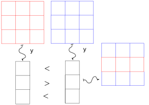
Figure 5.1: An illustration of the selection procedure defined in (5.49), for the simplified case of ${\bf f}^{\alpha}=\bm{0}$ for all $\alpha\in{\mathcal{A}}$ and $\#{\mathcal{A}}=2$. We multiply each matrix (red and blue in the figue) by the vector ${\bf y}$ and compare the components of the results. The matrix ${\bf K}^{{\bm{\alpha}}({\bf y})}$ is constructed by choosing the row of the matrix that gives the largest result.

1

input : Set ${\mathcal{A}}$.

Matrices $\{{\bf K}^{\alpha}\}_{\alpha\in{\mathcal{A}}}\subset\mathbb{R}^{N\times N}$.

Right hand sides $\{{\bf f}^{\alpha}\}_{\alpha\in{\mathcal{A}}}\subset\mathbb{R}^{N}$.

2

output : Vector ${\bf x}\in\mathbb{R}^{N}$, solution of (5.48).

3 Initialization: Choose ${\bf x}_{-1}\in\mathbb{R}^{N}$ ;

4 for $k\geq 0$ do

5       Set ${\bm{\alpha}}_{k}={\bm{\alpha}}({\bf x}_{k-1})$ ;

6       Compute ${\bf K}^{{\bm{\alpha}}_{k}}\in\mathbb{R}^{N\times N}$ and ${\bf f}^{{\bm{\alpha}}_{k}}\in\mathbb{R}^{N}$ ;

Find: ${\bf x}_{k}\in\mathbb{R}^{N}$ that solves

    $${𝐊}^{{𝜶}_k}{𝐱}_k={𝐟}^{{𝜶}_k}\text{ ;}$$ 7(5.50)

8       if  $k\geq 1$ and ${\bf x}_{k}={\bf x}_{k-1}$  then

9             return ${\bf x}_{k}$ ;

10            

11       end if

12      

13 end for

14

Algorithm 5.1 Howard’s algorithm.

Notice that, at each step, Algorithm 5.1 requires the solution to the linear system (5.50). Because of the way the matrices are constructed it is necessary to ensure that they are invertible. This is guaranteed by the following condition.

Assumption 5.51 (monotonicity).

For every ${\bf y}\in\mathbb{R}^{N}$ the matrix ${\bf K}^{{\bm{\alpha}}({\bf y})}$ is monotone in the sense of Definition 3.8.

It is natural to wonder when such a condition is satisfied. As shown in [135] if, for every $\alpha\in{\mathcal{A}}$, the matrix ${\bf K}^{\alpha}$ is strictly diagonally dominant and monotone and its off diagonal entries are nonpositive, then this condition is satisfied. We comment finally that a monotone matrix is nonsingular.

Having guaranteed that Howard’s algorithm can proceed, we focus our attention on its convergence. While many references have studied it, we will follow [16, 64] and draw a connection between this method and active set strategies which, in turn, can be analyzed as semismooth Newton methods. We begin with the definition of slant derivative.

Definition 5.52 (slant derivative).

Let $X$, and $Z$ be Banach spaces and $D\subset X$ be open. The mapping $F:D\to Z$ is called slantly differentiable in the open subset $U\subset D$ if there is a family of mappings $G:U\to\mathfrak{L}(X,Z)$ such that, for every $x\in U$,

$$\lim_{h\to 0}\frac{1}{\|h\|_{X}}\left\|F(x+h)-F(x)-G(x+h)h\right\|_{Z}=0.$$

We call $G$ a slanting function for $F$.

To approximate $x^{\star}\in X$, the solution of $F(x)=0$, one can then apply the semismooth Newton method which, starting from $x_{0}\in D$, computes iterates via:

$$x_{k+1}=x_{k}-G(x_{k})^{-1}F(x_{k}).$$ (5.53)

The convergence of (5.53) is given in the following result, whose proof can be found in [64, Theorem 1.1].

Theorem 5.54 (convergence).

Assume that $F$ is slantly differentiable in a neighborhood of $x^{\star}$. If $G(x)$ is nonsingular for all $x\in U$ and $\{\|G(x)^{-1}\|:x\in U\}$ is bounded, then the semismooth Newton method (5.53) converges superlinearly provided $x_{0}$ is sufficiently close to $x^{\star}$.

The connection between Howard’s algorithm and semismooth Newton methods is given by the following result; see [64, Lemma 3.1].

Lemma 5.55 (slant derivative of $\max$).

The mapping

$${\bf M}:\mathbb{R}^{N}\ni{\bf y}\mapsto\max\{\bm{0},{\bf y}\}\in\mathbb{R}^{N},$$

is slantly differentiable on $\mathbb{R}^{M}$ and a slanting function is

$${\bf G}_{\bf M}({\bf y})_{i,j}=g({\bf y}_{j})\delta_{i,j},\quad g(z)=\begin{dcases}0,&z\leq 0,\\ 1,&z>0.\end{dcases}$$

Let us explain how this result relates to Howard’s algorithm in the (perhaps overly) simplistic case that $N=1$, ${\mathcal{A}}=\{1,2\}$ and ${\bf f}^{1}={\bf f}^{2}={\bf f}$. In this setting, we are looking for ${\bf x}\in\mathbb{R}$ that solves

$$\bm{0}={\bf F}({\bf x})=\max\{{\bf K}^{1}{\bf x},{\bf K}^{2}{\bf x}\}-{\bf f}={\bf K}^{1}{\bf x}+\max\{\bm{0},({\bf K}^{2}-{\bf K}^{1}){\bf x}\}-{\bf f}.$$

By Lemma 5.55 a slanting function for ${\bf F}$ at ${\bf y}$ is

$${\bf G}({\bf y})={\bf K}^{1}+{\bf G}_{\bf M}\left(({\bf K}^{2}-{\bf K}^{1}){\bf y}\right)({\bf K}^{2}-{\bf K}^{1}).$$

If $({\bf K}^{2}-{\bf K}^{1}){\bf y}\geq 0$, then

$${\bf G}({\bf y})={\bf K}^{1}+({\bf K}^{2}-{\bf K}^{1})={\bf K}^{2},$$

and, similarly, if $({\bf K}^{2}-{\bf K}^{1}){\bf y}\leq 0$ we get ${\bf G}({\bf y})={\bf K}^{1}$. In other words, ${\bf G}({\bf y})$ always coincides with the coefficient that gives the largest result. Having made this observation, we can now establish convergence for Howard’s algorithm [16].

Theorem 5.56 (convergence).

If Assumption 5.51 is satisfied, then the sequence $\{{\bf x}_{k}\}_{k\geq 0}$, generated by Algorithm 5.1, satisfies ${\bf x}_{k}\geq{\bf x}_{k+1}$ for every $k\geq 0$ and converges to ${\bf x}$, the solution of (5.48). Moreover,

1. If $\#{\mathcal{A}}$ is finite, the sequence converges in at most $(\#{\mathcal{A}})^{N}$ steps.

2. If ${\mathcal{A}}$ is infinite, the convergence is asymptotically superlinear.

Proof.

To draw a connection between Algorithm 5.1 and the semismooth Newton method (5.53) let us sketch the proof. Recall that we are looking for a solution of (5.48), which can be understood as looking for a zero of the map ${\bf F}$. Let us now, following [16, Theorem 3.8], show that for ${\bf y}\in\mathbb{R}^{N}$ the matrix ${\bf K}^{{\bm{\alpha}}({\bf y})}$ is a slanting function for ${\bf F}$ at the point ${\bf y}$. For if that is the case, then (5.53) can be rewritten as

$${\bf K}^{{\bm{\alpha}}({\bf x}_{k})}\left({\bf x}_{k+1}-{\bf x}_{k}\right)=-{\bf F}({\bf x}_{k})=-{\bf K}^{{\bm{\alpha}}({\bf x}_{k})}{\bf x}_{k}+{\bf f}^{{\bm{\alpha}}({\bf x}_{k})},$$

which is clearly (5.50). By invoking Theorem 5.54 this will yield the superlinear convergence of $\{{\bf x}_{k}\}_{k\geq 0}$.

Now, to show the slant differentiability of ${\bf F}$, let ${\bf y},{\bf h}\in\mathbb{R}^{N}$ and notice that

$${\bf F}({\bf y})+{\bf K}^{{\bm{\alpha}}({\bf y}+{\bf h})}{\bf h} \geq{\bf K}^{{\bm{\alpha}}({\bf y}+{\bf h})}{\bf y}-{\bf f}^{{\bm{\alpha}}({\bf y}+{\bf h})}+{\bf K}^{{\bm{\alpha}}({\bf y}+{\bf h})}{\bf h}={\bf F}({\bf y}+{\bf h})$$

$$\geq{\bf K}^{{\bm{\alpha}}({\bf y})}({\bf y}+{\bf h})-{\bf f}^{{\bm{\alpha}}({\bf y})}={\bf F}({\bf y})+{\bf K}^{{\bm{\alpha}}({\bf y})}{\bf h}.$$

Consequently,

$$\bm{0} \geq{\bf F}({\bf y}+{\bf h})-{\bf F}({\bf y})-{\bf K}^{{\bm{\alpha}}({\bf y}+{\bf h})}{\bf h}\geq\left[{\bf K}^{{\bm{\alpha}}({\bf y})}-{\bf K}^{{\bm{\alpha}}({\bf y}+{\bf h})}\right]{\bf h}$$

$$\geq-|{\bf K}^{{\bm{\alpha}}({\bf y})}-{\bf K}^{{\bm{\alpha}}({\bf y}+{\bf h})}|_{\infty}|{\bf h}|_{\infty}.$$

Since Lemma 3.2 of [16] shows that $\lim_{|{\bf h}|_{\infty}\to 0}|{\bf K}^{{\bm{\alpha}}({\bf y})}-{\bf K}^{{\bm{\alpha}}({\bf y}+{\bf h})}|_{\infty}=0$ the result follows.

In the case $\#{\mathcal{A}}$ is finite we remark that the convergence in a finite number of steps follows from the monotonicity of the iterates. To show the monotonicity, we exploit the construction of the parameters ${\bm{\alpha}}_{k}$. Indeed, since

$${\bf K}^{{\bm{\alpha}}_{k+1}}{\bf x}_{k}-{\bf f}^{{\bm{\alpha}}_{k+1}}={\bf F}({\bf x}_{k})\geq{\bf K}^{{\bm{\alpha}}_{k}}{\bf x}_{k}-{\bf f}^{{\bm{\alpha}}_{k}}=\bm{0}={\bf K}^{{\bm{\alpha}}_{k+1}}{\bf x}_{k+1}-{\bf f}^{{\bm{\alpha}}_{k+1}},$$

we conclude that ${\bf K}^{{\bm{\alpha}}_{k+1}}\left({\bf x}_{k}-{\bf x}_{k+1}\right)\geq 0$. From Assumption 5.51 we have that ${\bf K}^{{\bm{\alpha}}_{k+1}}$ is monotone and, therefore, ${\bf x}_{k}\geq{\bf x}_{k+1}$. This concludes the proof. ∎

We conclude by commenting that, in Algorithm 5.1, at every step it is necessary to solve the linear system of equations (5.50) which, for large $N$, can be very time consuming. We refer to [66] where a multilevel technique to solve this problem is described and its global convergence is shown. Variations of this multigrid strategy are explored in [1] and [62]. Numerical methods of penalty type are studied in [135] and [96, Algorithme III].

6 The Monge-Ampère equation

The focus of this section is the study of discretizations for a particular convex equation: the Monge-Ampère equation with Dirichlet boundary conditions:

$$\begin{dcases}\det(D^{2}u)=f,&\text{in }\Omega,\\ u=g,&\text{on }\partial\Omega.\end{dcases}$$ (6.1)

The Monge-Ampère equation finds relevance in several areas of mathematics and its applications, including differential geometry, calculus of variations, economics, meteorology, and the optimal mass transportation problem [61, 129, 132, 10, 11, 125]. As we have already mentioned, see also Remark 6.17 below, the Monge-Ampère problem fits into the framework of the previous section. However, due to its many applications, and correspondingly its many discretizations and convergence results, we find it appropriate to devote an entire section to a sample of detailed results. Before discussing these methods, let us here give a brief synopsis of some discretizations for the Monge-Ampère problem that we do not cover in detail.

1. Monotone, wide-stencil finite difference schemes: [114, 54, 53, 13] The basis of these methods is to use determinant identities (such as Hadamard’s inequality) to construct consistent and monotone finite difference schemes for the Monge-Ampère problem. Such schemes conform to the Barles-Souganidis theory under certain assumptions and convergence to the viscosity solution is immediate. We refer the reader to [112] where rates of convergence for these methods have recently been derived.

2. Regularization: In [48, 47, 105, 49] the Monge-Ampère equation is first approximated at the continuous level by a fourth-order quasi-linear PDE. In this framework, solutions are defined via variational principles, and therefore Galerkin methods are readily constructed. Error estimates between the finite element approximation and the regularized solution are derived, but a general convergence theory for viscosity solutions is an open problem.

3. Variational methods: Classical Galerkin methodologies are used in references like [15, 19, 20, 106, 3, 2, 4] to construct finite element approximations for strong or classical solutions of the Monge-Ampère equation. Assuming that the solution to (6.1) is sufficiently regular error estimates are typically derived in $H^{1}$ or $H^{2}$-type norms.

4. Optimal control: In [34, 35], the Monge-Ampère equation is treated as a constraint of a minimization problem, leading to a saddle-point reformulation. Computationally efficient algorithms are proposed, but convergence to the viscosity solution is not shown.

We refer to the review paper [43] for a summary of these discretization types.

6.1 Solution concepts

The Monge-Ampère equation has a very unique structure and, because of this, the solution to problem (6.1) can be understood not only with the concepts described in Section 2, but with some additional ones. To discuss these issues, we first make the (sometimes necessary) assumption that the domain $\Omega$ is convex. With this assumption, and with an abuse of notation, we (re)define the convex envelope of a function $v$ with $v=0$ on $\partial\Omega$ as

$$\Gamma(v)(x):=\sup\left\{L(x):\ L(z)\leq v(z)\ \forall z\in\Omega,\ L\in\mathbb{P}_{1}\right\}.$$

As we previously described, in contrast to the problems discussed thus far, the Monge-Ampère operator $F(x,r,{\bf p},M):=\det(M)-f(x)$ is not elliptic on $\Omega\times\mathbb{R}\times\mathbb{R}^{d}\times\mathbb{S}^{d}$ (cf. Definition 2.15 and Example 2.19). Indeed, there holds

$$\det(M)\leq\det(N)\qquad\forall N\geq M$$

if and only if $M\geq 0$, and consequently $F$ is only elliptic restricted to the class of semi-positive definite matrices. In particular, if a classical solution $u$ to (6.1) exists, then $F$ is elliptic at $u$ if and only if $D^{2}u\geq 0$ in $\Omega$, implying that $u$ is a convex function. Further note that, besides ensuring ellipticity, the convexity assumption is required to have any hope of uniqueness, since, when $d$ is even

$$\det(D^{2}(-u))=\det(D^{2}u).$$

Let us now discuss the existence and uniqueness of different types of solutions of the Monge-Ampère problem (6.1) and the required conditions on the domain $\Omega$ and data, $f$ and $g$, to guarantee that such solutions exist. First we have the following result regarding classical solutions. [134, 130].

Theorem 6.2 (classical solutions).

Suppose that $\Omega$ is an open, bounded, and strictly convex domain with boundary $\partial\Omega\in C^{3}$. Suppose that $g\in C^{3}(\bar{\Omega})$, $f\in C^{\alpha}(\Omega)$ for some $\alpha\in(0,1)$, and that $\min_{\bar{\Omega}}f>0$. Then there exists a unique (classical) convex solution $u\in C^{2,\alpha}(\Omega)$ satisfying (6.1).

Remark 6.3 (optimality).

The conditions on $\partial\Omega$, $g$, and $f$ stated in Theorem 6.2 are optimal [130].

Next we turn our attention to viscosity solutions to (6.1). Since the operator $F$ is only elliptic on the class of convex functions, we must modify the definition of viscosity solutions to reflect this fact.

Definition 6.4 (viscosity solution).

A function $u\in C(\bar{\Omega})$ is called a viscosity subsolution (resp., supersolution) of (6.1) on the set of convex functions if $u$ is convex and if for all convex $\varphi\in C^{2}(\Omega)$ such that $u-\varphi$ has a local maximum (resp., minimum) at $x_{0}\in\Omega$, we have $\det(D^{2}\varphi(x_{0}))\geq f(x_{0})$ (resp., $\det(D^{2}\varphi(x_{0}))\leq f(x_{0})$). A function $u\in C(\bar{\Omega})$ is a viscosity solution to (6.1) on the class of convex functions if it is simultaneously a viscosity subsolution and super solution on the set of convex functions.

Remark 6.5 ($f$ is nonnegative).

Note that the definition of viscosity solution implicitly requires the source function $f$ to be continuous and nonnegative.

Before stating existence and uniqueness results for viscosity solutions let us, following [54], give an example of a non-classical viscosity solution. Note that this example shows that $f\in C^{\alpha}(\Omega)$ and smooth $\Omega$ is not sufficient to guarantee the existence of a classical solution.

Example 6.6 (viscosity solution).

Let $\Omega=B_{2}(0)\subset\mathbb{R}^{2}$, and consider the function

$$u(x)=\left\{\begin{array}[]{ll}0&\text{in $|x|\leq 1$},\\ \frac{1}{2}\big{(}|x|-1\big{)}^{2}&\text{in $1\leq|x|\leq 2$}.\end{array}\right.$$ (6.9)

Then $u$ is a viscosity solution of (6.1) with $g=1/2$ and

$$f(x)=\left\{\begin{array}[]{ll}0&\text{in $|x|\leq 1$},\\ 1-|x|^{-1}&\text{in $1\leq|x|\leq 2$}.\end{array}\right.$$

Theorem 6.10 (existence).

Assume that $\Omega$ is convex. Assume further that $g\in C(\partial\Omega)$, $f\in C(\bar{\Omega})$ and $f\geq 0$. Then there exists a unique viscosity solution $u\in C(\bar{\Omega})$ to (6.1) in the class of convex functions.

Apart from the viscosity solution, another notion of weak solution of the Monge-Ampère equation is based on geometric arguments, which we now describe. To motivate it, suppose for the moment that $f$ is uniformly positive in $\Omega$ and that $u\in C^{2}(\bar{\Omega})$ is a strictly convex function satisfying (6.1) pointwise. Let $\partial u(x)$ denote the subdifferential of $u$ at the point $x\in\Omega$ given by Definition 2.78, i.e., $\partial u(x)$ is the set of slopes of the supporting hyperplanes at $x$. From the convexity and smoothness assumptions we infer that $\partial u(x)=\{Du(x)\}$ and that the subdifferential, viewed as a map from $\Omega$ to $\mathbb{R}^{d}$, is injective. Consequently, a change of variables reveals that

$$\int_{D}f=\int_{D}\det(D^{2}u)=\int_{\partial u(D)}=|\partial u(D)|\quad\text{for all Borel sets }D\subset\Omega,$$

where we recall that $\partial u(D)=\cup_{x\in D}\partial u(x)$ and $|\partial u(D)|$ is the $d$-dimensional Lebesgue measure of $\partial u(D)$. Since $\partial u$ is well-defined for non-smooth convex functions, the above identity allows us to widen the class of admissible solutions.

Definition 6.11 (Alexandrov solution).

A convex function $u\in C(\bar{\Omega})$ is an Alexandrov solution to (6.1) if $u|_{\partial\Omega}=g$ and

$$|\partial u(D)|=\int_{D}f$$ (6.12)

for all Borel sets $D\subset\Omega$.

Note that the continuity of the source term $f$ is no longer required for (6.12) to be well-defined. The following example illustrates this feature.

Example 6.13 (Alexandrov solution).

Let $\Omega=B_{1}(0)\subset\mathbb{R}^{2}$. Then the function

$$u(x)=|x|-1$$

is a Alexandrov solution of Monge-Ampère equation

$$\det(D^{2}u)(x)=\pi\delta_{(x=0)},$$

where $\delta_{(x=0)}$ is the Dirac measure at origin. However, $u$ is not a viscosity solution because the right hand side is not a (continuous) function.

The existence and uniqueness of Alexandrov solutions is summarized in the next theorem, see [61, Theorem 1.6.2].

Theorem 6.14 (existence of Alexandrov solutions).

Let $\Omega\subset\mathbb{R}^{d}$ be an open, bounded, and strictly convex domain. Suppose that the data satisfies $g\in C(\partial\Omega)$ and $\int_{\Omega}f<\infty$. Then there exists a unique Alexandrov solution $u\in C(\bar{\Omega})$ to (6.1) in the class of convex functions.

The next result states situations where viscosity solutions and Alexandrov solutions coincide [61, Propositions 1.3.4 and 1.7.1]. The result also shows that the notion of Alexandrov solution is strictly weaker than that of a viscosity solution.

Proposition 6.15 (equivalence).

Suppose that $u\in C(\bar{\Omega})$ is an Alexandrov solution to (6.1). Then if $f$ is continuous, $u$ is a viscosity solution to (6.1). Conversely, if $u$ is a viscosity solution to (6.1) and if $f\in C(\bar{\Omega})$ with $f>0$ in $\bar{\Omega}$, then $u$ is an Alexandrov solution.

The rest of our presentation will deal separately with numerical methods for (6.1) depending on the type of solution we aim to approximate: viscosity or Alexandrov solutions. Before we discuss them, it is useful to review a property of the determinant. For convenience of notation we define the set of symmetric nonnegative definite matrices as

$$\mathbb{S}^{d}_{+}:=\{A\in\mathbb{S}^{d}:\ A\geq 0\}.$$

Proposition 6.16 (determinant inequality).

The following inequality holds:

$$\det(A)^{1/d}\det(B)^{1/d}\leq\frac{1}{d}\operatorname*{tr}AB=\frac{1}{d}(A:B)\qquad\forall A,B\in\mathbb{S}^{d}_{+}$$

with equality holding if and only if $B^{1/2}AB^{1/2}=cI$ for some scalar $c\geq 0$.

Proof.

Let $C=B^{1/2}AB^{1/2}$, and note that $C\in{\mathbb{S}}^{d}_{+}$. The arithmetic-geometric inequality yields

$$\det(C)^{1/d}\leq\frac{1}{d}\operatorname*{tr}C,$$

with equality holding if and only if $B^{1/2}AB^{1/2}=C=cI$. Since $A,B\in\mathbb{S}_{+}^{d}$ we find that $c\geq 0$. The inequality follows from the algebraic identities $\det C=\det(AB)=\det A\det B$ and $\operatorname*{tr}C=\operatorname*{tr}AB=A:B$. ∎

Remark 6.17 (Monge-Ampère is concave).

The determinant inequality of Proposition 6.16 implies that for any positive definite matrix $A$,

$$\det(A)^{1/d}=\inf_{B\in\mathbb{S}^{d}_{+}}\left\{\frac{1}{d}\operatorname*{tr}AB:\;\det B=1\right\}.$$

Therefore, for any symmetric positive definite $A$ and $B\in\mathbb{S}_{+}^{d}$, and for $0<t\leq 1$, we have

$$\det(tA+(1-t)B)^{1/d}= \;\inf_{K\in\mathbb{S}^{d}_{+}}\{\frac{1}{d}\operatorname*{tr}\left((tA+(1-t)B)K\right):\;\det K=1\}$$

$$\geq \;t\inf_{K\in\mathbb{S}^{d}_{+}}\{\frac{1}{d}\operatorname*{tr}(AK):\;\det K=1\}$$

$$\;+(1-t)\inf_{K\in\mathbb{S}^{d}_{+}}\{\frac{1}{d}\operatorname*{tr}(BK):\;\det K=1\}$$

$$= \;t\det(A)^{1/d}+(1-t)\det(B)^{1/d}.$$

The inequality $\det(tA+(1-t)B)^{1/d}\geq t\det(A)^{1/d}+(1-t)\det(B)^{1/d}$ is also satisfied if $t=0$, and if $\det(A)=\det(B)=0$. Thus the function $A\to\det A^{1/d}$ is concave over ${\mathbb{S}}^{d}_{+}$.

6.2 Approximation of viscosity solutions: Hamilton-Jacobi-Bellman reformulation

In this section we summarize the results of [45], where a numerical method based on a HJB reformation of the Monge-Ampère problem is developed. Before stating the method we first note that Remark 6.15 implicitly gives such a HJB reformation, i.e., if $u$ satisfies the first equation in (6.1), then formally

$$f(x)^{1/d}=\big{(}\det(D^{2}u)(x)\big{)}^{1/d}=\frac{1}{d}\mathop{\inf_{B\in\mathbb{S}^{d}_{+}}}_{\det(B)=1}D^{2}u(x):B.$$

Note that the constraint in the control set is nonlinear, and furthermore, the control set is not compact; these two features make the PDE and numerical constructions less obvious. Rather, the method proposed in [45] is based on the following result [83].

Proposition 6.18 (HJB reformulation of MA).

Define

$$\mathbb{S}^{d}_{1}=\{A\in\mathbb{S}^{d}_{+}:\ {\rm tr}\,A=1\},$$

and let $f\in\mathbb{R}$ with $f\geq 0$. Then a matrix $A\in\mathbb{S}^{d}$ satisfies

$$H(A,f):=\sup_{B\in\mathbb{S}^{d}_{1}}\Big{(}-\frac{1}{d}B:A+f^{1/d}\det(B)^{1/d}\Big{)}=0$$ (6.19)

if and only if $\det(A)=f$ and $A\in\mathbb{S}_{+}^{d}$. Moreover, there exists a maximizer $B_{*}\in\mathbb{S}^{d}_{1}$ that commutes with $A$.

Proof.

If $A\in\mathbb{S}^{d}_{+}$ and $\det(A)=f$, then Proposition 6.16 implies

$$-\frac{1}{d}B:A+f^{1/d}\det(B)^{1/d}\leq(f^{1/d}-\det(A)^{1/d})\det(B)^{1/d}=0$$

and equality holds if and only if $B^{1/2}AB^{1/2}=cI$ for some $c\geq 0$. If $A>0$ then we take $B=A^{-1}/\left(\operatorname*{tr}A^{-1}\right)$. Otherwise, if $\det(A)=0$, we use the eigendecomposition of a matrix to construct $B\in\mathbb{S}_{+}^{d}$ that commutes with $A$, $\operatorname*{tr}B=1$, and $B^{1/2}AB^{1/2}=0$. In either case we conclude that $A$ satisfies (6.19).

Now our goal is to show that (6.19) implies that $\det(A)=f$ and $A\in\mathbb{S}_{+}^{d}$. We prove the statement in two cases.

Case I. If $A>0$, then take $B=cA^{-1}$ with $c=1/(\operatorname*{tr}A^{-1})$ in (6.19). Using the identities $\frac{1}{d}B:A=c$ and $\det(B)=c^{d}\det(A)^{-1}$, we find that

$$c(f^{1/d}-\det(A)^{1/d})\det(A)^{-1/d}=\frac{-1}{d}B:A+f^{1/d}\det(B)^{1/d}\leq 0$$

and therefore $\det(A)\geq f$. On the other hand Proposition 6.16 implies that

$$0=\sup_{B\in\mathbb{S}^{d}_{1}}\Big{(}-\frac{1}{d}B:A+f^{1/d}\det(B)^{1/d}\Big{)}\leq\sup_{B\in\mathbb{S}^{d}_{1}}(f^{1/d}-\det(A)^{1/d})\det(B)^{1/d}.$$

Now if $\det(A)>f$, then we must have $\det(B)=0$ for the matrix $B$ to attain the supremum. However, since $A>0$, Proposition 6.16 implies the inequality above is strict if $B\neq cA^{-1}$. This leads to a contradiction. Therefore $\det(A)=f$. This proves the first case.

Case II: If $A$ is not strictly positive definite, then without loss of generality, we we assume that $A$ is of the diagonal form

$$A=\lambda_{1}{\bf v}_{1}\otimes{\bf v}_{1}+\cdots+\lambda_{d}{\bf v}_{d}\otimes{\bf v}_{d}\qquad\lambda_{1}\leq\cdots\leq\lambda_{d},$$

where $\{{\bf v}_{i}\}_{i=1}^{d}$ are the eigenvectors of $A$ with unit length, and $\lambda_{1}\leq 0$.

Consider the matrix

$$B=(1-\epsilon){\bf v}_{1}\otimes{\bf v}_{1}+\frac{\epsilon}{d-1}\sum_{i=2}^{d}{\bf v}_{i}\otimes{\bf v}_{i}\in\mathbb{S}^{d}_{1}$$

for some parameter $\epsilon\in(0,1)$. We then have

$$-\frac{1}{d}B:A+f^{1/d}\det(B)^{1/d} =-\frac{1}{d}\Big{(}(1-\epsilon)\lambda_{1}+\frac{\epsilon}{d-1}\sum_{i=2}^{d}\lambda_{i}\Big{)}$$

$$\qquad+(1-\epsilon)^{1/d}\frac{\epsilon^{(d-1)/d}}{(d-1)^{(d-1)/d}}f^{1/d}$$

$$\geq\frac{-1}{d}\left((1-\epsilon)\lambda_{1}+\epsilon\lambda_{d}\right)+\left[\frac{(1-\epsilon)\epsilon^{(d-1)}}{(d-1)^{(d-1)}}f\right]^{1/d}.$$

Note that if $f>0$ and for sufficiently small $\epsilon$, the dominating term is $\left[\frac{(1-\epsilon)\epsilon^{(d-1)}}{(d-1)^{(d-1)}}f\right]^{1/d}$. Thus, if $f>0$, then we deduce

$$-\frac{1}{d}B:A+f^{1/d}\det(B)^{1/d}>0$$

which contradicts (6.19). If $f=0$, then

$$-\frac{1}{d}B:A+f^{1/d}\det(B)^{1/d}=-\frac{1}{d}\Big{(}(1-\epsilon)\lambda_{1}+\frac{\epsilon}{d-1}\sum_{i=2}^{d}\lambda_{i}\Big{)}.$$

Equation (6.19) holds for any $\epsilon>0$ if and only if $\lambda_{1}=0$. Thus, $A\geq 0$ and $\det(A)=f=0$. This completes the proof. ∎

Lemma 6.18 leads to the following result, showing that viscosity solutions to the Monge-Ampère equation are viscosity solutions of a HJB problem. We refer the reader to [45, Theorem 3.3] for a proof.

Theorem 6.20 (equivalence of viscosity solutions).

Let $f\in C(\Omega)$ be a non-negative function, and let $u$ be a viscosity subsolution (resp., supersolution) of the Monge-Ampère problem (6.1) on the set of convex functions. Then $u$ is a viscosity subsolution (resp., supersolution) to the HJB problem

$$\begin{dcases}H(D^{2}u,f)=0&\text{in }\Omega,\\ u=g&\text{on }\partial\Omega.\end{dcases}$$ (6.21)

Remark 6.22 (convexity of solution).

We emphasize that the convexity of the solution to (6.21) is not assumed a priori; it occurs implicitly from the structure of the HJB problem.

Remark 6.23 (${\mathbb{S}}^{d}_{1}$ is not Cordes).

It is worth mentioning that matrices in $\mathbb{S}_{1}^{d}$ do not necessarily satisfy the Cordes condition if $d\geq 3$ (cf. Definition 2.46). To see this, consider $B\in\mathbb{S}_{1}^{3}$ with eigenvalues $\lambda_{1}=1-\tau$, $\lambda_{2}=\lambda_{3}=\frac{\tau}{2}$ for some $\tau\in(0,\frac{1}{3}]$. We then find

$$\frac{|B|^{2}}{({\rm tr}\,B)^{2}}=\lambda_{1}^{2}+\lambda_{2}^{2}+\lambda_{3}^{2}=\frac{3}{2}\tau^{2}-2\tau+1\geq\frac{1}{2},$$

and thus, $B$ does not satisfy the Cordes condition.

6.2.1 Discretization of the HJB-reformulation

To describe a discretization method for problem (6.21), we first note that if $B\in\mathbb{S}^{d}_{1}$, then $B=YDY^{\intercal}$, where $D\in\mathbb{S}^{d}_{1}$ is a diagonal matrix and $Y=[{\bf y}_{1},\cdots,{\bf y}_{d}]\in\mathbb{SO}^{d}$, where $\mathbb{SO}^{d}$ is the special orthogonal group. Thus, denoting by $\mathbb{D}^{d}_{1}$ the space of diagonal nonnegative definite matrices with unit trace, we find that

$$H(A,f)=\mathop{\sup_{Y\in\mathbb{SO}^{d}}}_{D\in\mathbb{D}_{1}^{d}}\Big{(}-\frac{1}{d}YDY^{\intercal}:A+f^{1/d}\det(D)^{1/d}\Big{)}.$$

Let ${\bf y}_{i}\in\mathbb{R}^{d}$ denote the $ith$ column of $Y\in\mathbb{SO}^{d}$ and let $\lambda_{i}=D_{i,i}$. Then the solution to the Monge-Ampère equation satisfies

$$\mathop{\sup_{Y\in\mathbb{SO}^{d}}}_{D\in\mathbb{D}_{1}^{d}}\Big{(}-\frac{1}{d}\sum_{i=1}^{d}\lambda_{i}{\bf y}_{i}\otimes{\bf y}_{i}:D^{2}u(x)+f(x)^{1/d}\Big{(}\prod_{i=1}^{d}\lambda_{i}\Big{)}^{1/d}\Big{)}=0$$

in the viscosity sense.

Let ${\mathcal{T}_{h}}$ be a quasi-uniform and shape regular mesh of $\Omega$ and $X^{l}_{h}$ be the continuous piecewise linear polynomials over ${\mathcal{T}_{h}}$ defined by (3.71). We denote by $\Omega_{h}^{I}$ the set of interior vertices of $\mathcal{T}_{h}$, and by $\Omega_{h}^{B}$ the set of boundary vertices. Let $v_{h}\in X^{l}_{h}$. Recall that, for a discretization parameter $k>0$ and vector $y$, the second order difference operator is defined by

$$\delta_{y,k}^{2}v_{h}(z)=\frac{1}{k^{2}}\big{(}v_{h}(z+ky)-2v_{h}(z)+v_{h}(z-ky)\big{)}$$

provided that $z$ is sufficiently far from the boundary, namely, $z\pm ky\in\bar{\Omega}$. Otherwise we set

$$\delta_{y,k}^{2}v_{h}(z)= \;\frac{2}{k^{+}+k^{-}}\left(\frac{v_{h}(z+k^{+}y)-v_{h}(z)}{k^{+}}+\frac{v_{h}(z-k^{-}y)-v_{h}(z)}{k^{-}}\right),$$

where $k^{\pm}$ is the only element in $(0,k]$ such that $z\pm k^{\pm}y\in\partial\Omega$.

With these definitions at hand we introduce, on $X^{l}_{h}$, the following approximation of the HJB reformulation

$$H_{h}^{k}[u_{h},f](z)=\mathop{\sup_{Y\in\mathbb{SO}^{d}}}_{D\in\mathbb{D}_{1}^{d}}\left(\frac{-1}{d}\sum_{i=1}^{d}\lambda_{i}\delta_{y,k}^{2}u_{h}(z)+f(z)^{1/d}\det(D)^{1/d}\right),$$

where $z\in\Omega_{h}^{I}$.

The numerical method based on the HJB reformulation seeks a piecewise linear function $u_{h}\in X^{l}_{h}$ such that

$$\begin{dcases}H^{k}_{h}[u_{h},f]=0&\text{in }\Omega_{h}^{I},\\ u_{h}=g&\text{on }\Omega_{h}^{B}.\end{dcases}$$ (6.24)

Note that, the boundary conditions uniquely determine $u_{h}$ on $\partial\Omega$, and therefore the problem is well-defined. The scheme (6.24) is a semi-Lagrangian method because the points $z\pm ky$, which are used to evaluate $\delta_{y,h}^{2}u_{h}(z)$, may not belong to $\bar{\Omega}_{h}$. Thus, additional effort is needed to evaluate $u_{h}(z\pm ky)$.

It is straightforward to check that $\delta_{y,k}^{2}u_{h}(z)$ is monotone for any direction $y$, implying that operator $H^{k}_{h}[u_{h},f]$ is monotone. The monotonicity also leads to stability of the method [45, Lemmas 6.2 and 6.4].

Lemma 6.25 (stability).

Problem (6.24) is stable in the sense that there exists a unique solution $u_{h}\in X^{l}_{h}$ to (6.24) and an $h$-independent constant $C>0$ such that $\|u_{h}\|_{L^{\infty}(\Omega)}\leq C$. Moreover if we set

$$\bar{u}(x):=\mathop{\limsup_{y\to x}}_{h\to 0^{+}}u_{h}(y),\quad\underline{u}(x):=\mathop{\liminf_{y\to x}}_{h\to 0^{+}}u_{h}(y),\quad x\in\bar{\Omega},$$

then $\bar{u}(x)=\underline{u}(x)=g(x)$ for all $x\in\partial\Omega$ provided that $\Omega$ is strictly convex.

To show the consistency of the method, we recall that $I_{h}^{fe}:C(\bar{\Omega})\to X^{l}_{h}$ denotes the nodal interpolant. We then have the following result.

Lemma 6.26 (consistency).

Let $\phi\in C^{2,\alpha}(\Omega)$, then there is a constant $C$ such that, for every $z\in\Omega_{h}^{I}$, we have

$$\left|H(D^{2}\phi(z),f(z))-H_{h}^{k}[I_{h}^{fe}\phi,f](z)\right|\leq C\left(k^{\alpha}+\frac{h^{2}}{k^{2}_{\min}}\right),$$

where $k_{\min}=\min\{k^{+},k^{-}\}$. Consequently, the method is consistent if $k\to 0$ and $\frac{h}{k_{\min}}\to 0$.

Proof.

It suffices to show that

$$|\delta_{y,k}^{2}I_{h}^{fe}\phi(z)-(y\otimes y):D^{2}\phi(z)|\leq C\left(k^{\alpha}+\frac{h^{2}}{k^{2}_{\min}}\right).$$

First, by Taylor’s Theorem, we have

$$\big{|}\delta_{y,k}^{2}\phi(z)-(y\otimes y):D^{2}\phi(z)\big{|}\leq Ck^{\alpha}\|\phi\|_{C^{2,\alpha}(\Omega)}.$$ (6.27)

Recalling that [29],

$$\|\phi-I_{h}^{fe}\phi\|_{L^{\infty}(\Omega)}\leq Ch^{2}\|\phi\|_{W^{2,\infty}(\Omega)},$$

we have

$$\big{|}\delta_{y,k}^{2}\phi(z)-\delta_{y,k}^{2}I_{h}^{fe}\phi(z)\big{|}\leq C\frac{h^{2}}{k_{\min}^{2}}\|\phi\|_{W^{2,\infty}(\Omega)}.$$ (6.28)

The desired result now follows from (6.27)–(6.28) and the triangle inequality. ∎

Remark 6.29 (discrete controls).

To implement the method (6.24), it remains to specify a discrete set $\mathbb{S}_{1,h}^{d}\subset\mathbb{S}_{1}^{d}$ of symmetric positive definite matrices with unit trace. To ensure consistency of the method, we require the discrete set $\mathbb{S}_{1,h}^{d}$ to be dense as $h\to 0$, that is, for any $B\in\mathbb{S}_{1}^{d}$, there is $B_{h}\in\mathbb{S}_{1,h}^{d}$ such that $B_{h}\to B$ as $h\to 0$.

Since the method is monotone and consistent, the convergence of the numerical solution now follows from the Barles-Souganidis theory (cf. Theorem 3.14 and [45, Theorem 6.5]).

Theorem 6.30 (convergence).

Let $\Omega\subset\mathbb{R}^{d}$ be a strictly convex domain. Assume that $f\in C(\Omega)$ with $f\geq 0$ and $g\in C(\partial\Omega)$. Then as $h\to 0$, $h/k_{\min}\to 0$, the solutions $u_{h}\in X^{l}_{h}$ of (6.24) converge uniformly to the unique viscosity solution on the set of convex functions of the Monge-Ampère problem (6.1).

We conclude the discussion on semi-Lagrangian schemes by commenting that rates of convergence for a general semi-Lagrangian scheme for (5.1) have been obtained in [36, Corollary 7.3].

6.3 Approximation of Alexandrov solutions

Now we discuss numerical methods based on the Alexandrov solution concept presented in Definition 6.11. Essentially, this class of numerical methods are finite dimensional analogues of (6.12).

Let $\{\omega_{i}\}_{i=1}^{N}$ be an open, disjoint partition of the domain, i.e., $\omega_{i}\cap\omega_{j}=\emptyset$ for $i\neq j$ and $\bar{\Omega}=\cup_{i=1}^{N}\bar{\omega}_{i}$. Let $\Omega_{h}^{I}:=\{z_{i}\}_{i=1}^{N}$ be a collection of points with the property that $z_{i}\in\omega_{j}$ if and only if $i=j$, and let $\Omega_{h}^{B}:=\{z_{i}\}_{i=N+1}^{M+N}$ be a set of distinct points on $\partial\Omega$. As before, we denote $\bar{\Omega}_{h}=\Omega_{h}^{I}\cup\Omega_{h}^{B}$ and we will call its elements nodes or grid points.

Recall that for a nodal function $v_{h}\in X_{h}^{fd}$, its subdifferential at a grid point $z\in\bar{\Omega}_{h}$ is given by (3.38). Now, a natural generalization of (6.12), and the discrete problem proposed in [116] reads: Find a convex nodal function $u_{h}\in X_{h}^{fd}$ satisfying

$$\begin{dcases}|\partial u_{h}(z_{i})|=\int_{\omega_{i}}f,&\forall z_{i}\in\Omega_{h}^{I},\\ u_{h}(z_{i})=g(z_{i}),&\forall z_{i}\in\Omega_{h}^{B}.\end{dcases}$$ (6.31)

Note that since the partition $\{\omega_{i}\}_{i=1}^{N}$ is non-overlapping, for all Borel sets $D\subset\Omega$ we have

$$|\partial u_{h}(D)|=\sum_{z_{i}\in D}f_{i},\qquad f_{i}=\int_{\omega_{i}}f.$$

Thus, the scheme is obtained by replacing $f$ in (6.12) by a family of Dirac measures supported at the nodes and by replacing $g$ by its nodal interpolant on the boundary.

One special case of this method is when the interior nodal set is a lattice, i.e., for some basis $\{\tilde{\bf e}_{j}\}_{j=1}^{d}$ of $\mathbb{R}^{d}$ we have

$$\Omega_{h}^{I}=\left\{z=h\sum_{j=1}^{d}z^{j}\tilde{\bf e}_{j}:z^{j}\in{\mathbb{Z}}\right\}\cap\Omega.$$

We remark that this property applies to interior nodes only. For the boundary nodes, we only require that their spacing is of order $h$, namely, $\partial\Omega\subset\cup_{z\in\Omega_{h}^{B}}B_{h/2}(z)$. In this case, the partition $\{\omega_{i}\}$ of the domain can be taken as parallelotopes

$$\omega_{i}=\left\{z_{i}+\sum_{j=1}^{d}h^{j}\tilde{\bf e}_{j}:\ h^{j}\in\mathbb{R},\ |h^{j}|\leq\frac{h}{2}\right\}\cap\Omega.$$ (6.32)

The length of the coordinate vectors $\{\tilde{\bf e}_{j}\}_{j=1}^{d}$ is such that the parallelotope $\omega_{i}$ is inside the ball $B_{h}(z_{i})$ centered at $z_{i}$ and of radius $h$. Notice that, by construction, $\omega_{j}=z_{j}-z_{i}+\omega_{i}$; consequently, the radius of the largest ball inscribed in $\omega_{i}$ does not depend on $i$ and we denote it by $\rho$. We define the shape-regularity of the nodal set as

$$\sigma=h\rho^{-1}.$$ (6.33)

Remark 6.34 (meshless nodal function).

It is worth mentioning again that the solution $u_{h}$ is only defined at the nodes $\bar{\Omega}_{h}$. Its convex envelope induces a triangulation of the domain $\Omega$ and a piecewise linear function. However, this triangulation is not known a priori. See Remark 3.36 and Examples 3.87–3.88.

In view of Example 3.88, if the solution of the Monge-Ampère equation is nearly degenerate, wide stencils are needed to compute the subdifferential. Thus, method (6.31) may be regarded as a wide stencil finite difference scheme when the solution is nearly degenerate. On the other hand, if the solution to (6.1) is strictly convex, i.e., for $0<\lambda\leq\Lambda$ we have $\lambda I\leq D^{2}u\leq\Lambda I$, then the sub-differential of $u_{h}$ at node $z$ depends only on the values of $u_{h}$ at the adjacent nodes of $z$. To make this last statement rigorous, we state a definition.

Definition 6.35 (adjacent set).

Let $u_{h}\in X_{h}^{fd}$ and $z\in\Omega^{I}_{h}$. The adjacent set $A_{z}$ of $u_{h}$ at $z$ is the collection of nodes $z_{i}\in\bar{\Omega}_{h}$ such that there exists a supporting hyperplane $\ell$ of $u_{h}$ at $z$ and $\ell(z_{i})=u_{h}(z_{i})$.

Note that $A_{z}$ is the set of nodes of a star of $z$ which is induced by the discrete convex envelope of $u_{h}$; see Figure 3.2. In particular, we have that the subdifferential $\partial u_{h}(z)$ is determined by the values $u(z_{i})$ for $z_{i}\in A_{z}$.

Let us now estimate the size of $A_{z}$.

Lemma 6.36 (size of $A_{z}$).

Let $v\in C^{2}(\bar{\Omega})$ be a strictly convex function with $\lambda I\leq D^{2}v(x)\leq\Lambda I$ for some constants $0<\lambda\leq\Lambda$. Assume that $E:=\{\tilde{\bf e}_{j}\}_{j=1}^{d}$ is a basis of $\mathbb{R}^{d}$ such that $\Omega_{h}^{I}$ is a lattice spanned by $E$ with shape regularity constant $\sigma$ defined in (6.33). Let the nodal function $v_{h}\in X_{h}^{fd}$ be defined by $v_{h}=I_{h}^{fd}v$. Then, if $A_{z}$ is the adjacent set of $v_{h}$ at $z\in\Omega_{h}^{I}$,

$$A_{z}\subset B_{Rh}(z),$$

where

$$R\geq\bar{R}:=\frac{\Lambda}{\lambda}\sigma^{2}\left|\sum_{j=1}^{d}\tilde{{\bf e}}_{j}\right|^{2}.$$ (6.37)

Proof.

Without loss of generality, we may assume that $z=0$, $v(z)=0$, and $Dv(z)=\bm{0}$. Let $\hat{z}\in\Omega_{h}^{I}\cap\partial\operatorname{conv}(A_{z})$ and $\omega$ be the parallelotope defined as in (6.32) with center $z=0$. By convexity of $\omega$, there is a $c\in(0,1)$ such that $c\hat{z}\in\partial\omega$. Thus, we can express $\hat{z}$ as a multiple of a convex combination of $\{\zeta_{j}\}_{j=1}^{2^{d}}$, the vertices of $\omega$. In other words, for $R=1/c$, we have

$$\hat{z}=R\sum_{j=1}^{2^{d}}k_{j}\zeta_{j},\quad k_{j}\geq 0,\quad\sum_{j=1}^{2^{d}}k_{j}=1.$$

This representation shows that $|\hat{z}|\leq Rh$; thus, to obtain the result, it remains to estimate $R$.

Since $c\hat{z}\in\partial\omega$ we have, using (6.33), that $|c\hat{z}|\geq\rho=h\sigma^{-1}$ which can be rewritten as $|\hat{z}|\geq Rh\sigma^{-1}$. Using that $D^{2}v\geq\lambda I$ we estimate

$$v_{h}(\hat{z})=v(\hat{z})\geq\frac{1}{2}\lambda R^{2}\sigma^{-2}h^{2}.$$

Let us now obtain an upper bound for $v_{h}(\hat{z})$. To do so, let us introduce $\hat{\omega}$ as the (unique) smallest parallelotope with vertices $\{\bar{z}_{m}\}_{m=1}^{2^{d}}\subset\Omega_{h}^{I}$ such that $z\in\{\bar{z}_{m}\}_{m=1}^{2^{d}}$ is a vertex and $c\hat{z}\in\hat{\omega}$. This parallelotope can be thought of as belonging to the dual mesh. We now invoke Caratheodory’s theorem [33, Theorem 2.13] to conclude that there is a subset of $\{\bar{z}_{m}\}_{m=1}^{2^{d}}$, of cardinality $d+1$, for which $c\hat{z}$ can be expressed as a convex combination of these vertices. In other words, up to a permutation in $\{1,\ldots,2^{d}\}$, we have

$$\hat{z}=R\sum_{m=1}^{d+1}\alpha_{m}\bar{z}_{m},\quad\alpha_{m}\geq 0,\quad\sum_{m=1}^{d+1}\alpha_{m}=1.$$ (6.38)

We now invoke that $\hat{z}\in A_{z}$. This implies that there is an affine function $\ell$ that verifies

$$\ell(z)=v_{h}(z)=0,\qquad\ell(\hat{z})=v_{h}(\hat{z}),\qquad\ell(\bar{z}_{m})\leq v_{h}(\bar{z}_{m}),\ m=1,\ldots,d+1.$$

Using representation (6.38) of $\hat{z}$ and that $D^{2}v\leq\Lambda I$ we then obtain

$$v_{h}(\hat{z})=R\sum_{m=1}^{d+1}\alpha_{m}\ell(\bar{z}_{m})\leq\frac{1}{2}\Lambda R\sum_{m=1}^{d+1}\alpha_{m}|\bar{z}_{m}|^{2}.$$

It remains to observe now that $\bar{z}_{m}=z+\sum_{j=1}^{d}\epsilon_{j}h\tilde{\bf e}_{j}$ with $\epsilon_{j}\in\{-1,0,1\}$ and, therefore,

$$|\bar{z}_{m}|\leq h\left|\sum_{j=1}^{d}\tilde{\bf e}_{j}\right|.$$

A combination of the obtained upper and lower bounds for $v_{h}(\hat{z})$ yields

$$\frac{1}{2}\lambda R^{2}h^{2}\sigma^{-2}\leq\frac{1}{2}\Lambda Rh^{2}\left|\sum_{j=1}^{d}\tilde{\bf e}_{j}\right|^{2},$$

from which (6.37) follows. ∎

Remark 6.39 (Cartesian lattice).

In the setting of Lemma 6.36, if $E$ is the canonical basis of $\mathbb{R}^{d}$ then [100, 12] have improved estimate (6.37) to $\bar{R}=\frac{\Lambda}{\lambda}\sigma^{2}$.

If $\Omega^{I}_{h}$ is a lattice, then we are able to show consistency of the method (6.31) in the following sense.

Lemma 6.40 (consistency).

Let $E=\{\tilde{\bf e}_{j}\}_{j=1}^{d}$ be a basis of $\mathbb{R}^{d}$ and $\Omega_{h}^{I}$ be a lattice spanned by $E$. Let $p$ be a strictly convex quadratic polynomial with $\lambda I\leq D^{2}p\leq\Lambda I$. If $z\in\Omega_{h}^{I}$ is such that $\operatorname{dist}(z,\partial\Omega)\geq\bar{R}h$, with $\bar{R}$ as in (6.37), then we have

$$|\partial I_{h}^{fd}p(z)|=\det(D^{2}p)|\omega_{z}|,$$ (6.41)

where $\omega_{z}$ is the parallelotope defined by (6.32).

Proof.

We divide the proof in two steps.

Step 1. We first show that (6.41) holds when the domain is $\Omega=\mathbb{R}^{d}$. Without loss of generality, we assume that $z=0$ and $p(x)=\frac{1}{2}x\cdot Mx$ for some $M\geq\lambda I$. For a vector ${\bf q}\in\mathbb{R}^{d}$ we define the norm $|{\bf q}|_{M}^{2}:={\bf q}\cdot M{\bf q}$, and define the set

$$V :=\{{\bf q}\in\mathbb{R}^{d}:|{\bf q}|_{M}\leq|{\bf q}-z_{j}|_{M},\ \forall z_{j}\in\bar{\Omega}_{h}\}$$

$$=\left\{{\bf q}\in\mathbb{R}^{d}:{\bf q}\cdot Mz_{j}\leq\frac{1}{2}z_{j}\cdot Mz_{j},\ \forall z_{j}\in\bar{\Omega}_{h}\right\}.$$

It can be shown, see [100, Lemma 2.3] for details, that translations of $V$ tile $\mathbb{R}^{d}$ and that $|V|=|\omega_{z}|$. Moreover, by a simple algebraic manipulation,

$$V=\{M^{-1}{\bf q}\in\mathbb{R}^{d}:{\bf q}\cdot z_{j}\leq I_{h}^{fd}p(z_{j}),\ \forall z_{j}\in\bar{\Omega}_{h}\}.$$

Thus, $V=M^{-1}[\partial I_{h}^{fd}p(0)]$, i.e., it is the image of subdifferential $\partial I_{h}^{fd}p(0)$ under the linear map $M^{-1}$. Taking measure on both sides yields

$$|\omega_{z}|=|V|=\det(M)^{-1}|\partial I_{h}^{fd}p(0)|.$$

The proof of step 1 is now completed by rearranging terms.

Step 2. We now consider a bounded domain and show that (6.41) holds for nodes sufficiently far away from the boundary , i.e., $\operatorname{dist}(z,\partial\Omega)\geq\bar{R}h$. To do so, we observe that the subdifferential $\partial I_{h}^{fd}p(z)$ is determined only by the function values in the adjacent set $A_{z}$. Since, as shown in Lemma 6.36, $A_{z}\subset B_{\bar{R}h}(z)$ we deduce that if the node $z$ is bounded away from the boundary with $\operatorname{dist}(z,\partial\Omega)\geq\bar{R}h$, then $A_{z}\subset\Omega$. Thus, (6.41) holds.

This concludes the proof. ∎

6.3.1 A truncated version

In the case $\Omega_{h}^{I}$ is a Cartesian lattice, scheme (6.31) is is closely related with the finite difference method of [100, 12] which we now describe. For simplicity, suppose that $d=2$ and that the interior grid points are given by

$$\Omega_{h}^{I}=\Omega\cap\mathbb{Z}^{2}_{h}.$$

Let $S\subset\mathbb{Z}^{2}\backslash\{0\}$ denote a stencil. For any $y\in S$ and $z\in\Omega_{h}^{I}$ sufficiently far from $\partial\Omega$, we recall that the second-order difference operator in the direction $y$ is given by

$$\delta_{y,h}^{2}v(z)=\frac{v(z+hy)-2v(z)+v(z-hy)}{h^{2}}.$$

When $z\in\Omega_{h}^{I}$ is close to $\partial\Omega$, the point $z\pm hy$ may not belong to $\bar{\Omega}_{h}$. In such cases, we define

$$\delta^{2}_{y,h}v(z):=\frac{2}{h^{+}+h^{-}}\left(\frac{v(z+h^{+}y)-v(z)}{h^{+}}+\frac{v(z-h^{-}y)-v(z)}{h^{-}}\right),$$

where $h^{\pm}$ is the only element in $[0,h]$ such that $z\pm h^{\pm}y\in\partial\Omega$. This construction implicitly defines the set of boundary points $\Omega_{h}^{B}$.

We define the set of superbases of $S$ as

$$Y_{h}:=\left\{(y_{0},y_{1},y_{2})\in S^{3}:\ |\det(y_{0},y_{1},y_{2})|=1,\ y_{0}+y_{1}+y_{2}=\bm{0}\right\}.$$

Note that for $z\in\Omega_{h}^{I}$ and ${\bf y}=(y_{0},y_{1},y_{2})\in Y_{h}$, the convex hull ${\mathcal{H}}_{z,{\bf y}}=\operatorname{conv}\{z\pm hy_{i}\}_{i=0}^{3}$ is a hexagon. Given a nodal function $v_{h}$, superbasis ${\bf y}=(y_{0},y_{1},y_{2})\in Y_{h}$, and a point $z\in\Omega_{h}^{I}$, we denote by $\Gamma_{z,{\bf y}}(v_{h})$ the maximal convex map bounded above by $v_{h}$ at the points $z$ and $\{z\pm hy_{i}\}_{i=0}^{3}$. As before $\Gamma_{z,{\bf y}}(v_{h})$, restricted to ${\mathcal{H}}_{z,{\bf y}}$, is a piecewise linear function with respect to some triangulation of ${\mathcal{H}}_{z,{\bf y}}$, which depends on the values of $v_{h}$ on the extreme points of ${\mathcal{H}}_{z,{\bf y}}$ and $z$.

We define the discrete Monge-Ampère operator

$$\gamma(\Delta^{+}_{y_{0}}v_{h}(z),\Delta^{+}_{y_{1}}v_{h}(z),\Delta^{+}_{y_{2}}v_{h}(z)),$$

with $\Delta_{y}^{+}v(z)=\max\{\delta_{y,h}^{2}v_{h}(z),0\}$ and

$$\gamma(\delta_{0},\delta_{1},\delta_{2}):=\left\{\begin{array}[]{ll}\delta_{i+1}\delta_{i+2}&\text{if }\delta_{i}\geq\delta_{i+1}+\delta_{i+2},\ i=0,\ldots,2\mod 3,\\ \gamma_{1}(\delta_{0},\delta_{1},\delta_{2})&\text{otherwise},\end{array}\right.$$

with $\gamma_{1}(\delta_{0},\delta_{1},\delta_{2}):=\frac{1}{2}(\delta_{0}\delta_{1}+\delta_{1}\delta_{2}+\delta_{0}\delta_{2})-\frac{1}{4}(\delta_{0}^{2}+\delta_{1}^{2}+\delta_{2}^{2})$. As shown in [12, Remark 1.10], from the definition of subdifferential and some geometric arguments it follows that

$$\gamma(\Delta^{+}_{y_{0}}v_{h}(z),\Delta^{+}_{y_{1}}v_{h}(z),\Delta^{+}_{y_{2}}v_{h}(z))=h^{2}|\partial\Gamma_{z,{\bf y}}(v_{h})(z)|.$$

The scheme proposed in [12] reads: Find the nodal function $u_{h}\in X_{h}^{fd}$ such that

$$\begin{dcases}\min_{{\bf y}\in Y_{h}}\gamma(\Delta^{+}_{y_{0}}u_{h}(z),\Delta^{+}_{y_{1}}u_{h}(z),\Delta^{+}_{y_{2}}u_{h}(z))=f(z),&\forall z\in\Omega_{h}^{I},\\ u_{h}(z)=g(z),&\forall z\in\Omega_{h}^{B}.\end{dcases}$$ (6.42)

Lemma 6.43 (consistency).

Let $M$ be a positive definite matrix and $p(x)=\frac{1}{2}x\cdot Mx$ be a convex quadratic polynomial. Then

$$\min_{{\bf y}\in Y_{h}}|\partial\Gamma_{z,{\bf y}}(I^{fd}_{h}p)(z)|=\det(M)$$

if and only if there is a $M$-obtuse superbasis $(y_{0},y_{1},y_{2})$, that is,

$$y_{i}\cdot My_{j}\leq 0\quad\forall i\neq j.$$

Moreover, if $B_{R}\subset\operatorname{conv}S$ with $R^{2}=2|{M}||{M^{-1}}|$, then such a $M$-obtuse basis exists in $S$.

We refer to [12, Propositions 1.12 and 2.2] for a proof. Notice that the previous result shows that if the matrix $M$ is anisotropic, i.e., $|M||M^{-1}|$ is large, then a wide stencil is needed to ensure the existence of a $M$-obtuse superbasis.

Remark 6.44 (three dimensions).

In three space dimensions, to the best of our knowledge, there is no explicit formula to compute $|\partial\Gamma_{z,{{\bf y}}}(v_{h})(z)|$. As shown in [100], if $p(x)=\frac{1}{2}x\cdot Mx$ and the stencil $S$ is such that $B_{R}\subset\operatorname{conv}S$, for some $R$ that depends on $|M||M^{-1}|$, then we have that

$$\det(M)=h^{3}|\partial\Gamma_{z,{\bf y}}(I^{fd}_{h}p)(z)|.$$

This result is consistent with Lemma 6.40.

6.3.2 Stability of (6.31)

While the convergence of monotone and consistent schemes, like (6.31), can be obtained using the framework described in Section 3.1, few results are known on the rate of convergence of such approximations. Here we discuss, following [112], some recent results on the $L^{\infty}$-rate of convergence of scheme (6.31).

The derivation of these error estimates involves, in addition to the discrete Alexandrov estimates of Lemmas 3.44 and 3.89, a discrete barrier argument as in Section 4.3 and the Brunn-Minkowski inequality, which we now state.

Let $D$ and $E$ be two nonempty compact subsets of $\mathbb{R}^{d}$. We define their (Minkowski) sum as

$$D+E:=\left\{{\bf v}+{\bf w}\in\mathbb{R}^{d}:{\bf v}\in D\ {\bf w}\in E\right\}.$$

Proposition 6.45 (Brunn-Minkowski).

Let $A$ and $B$ be two nonempty compact subsets of $\mathbb{R}^{d}$. Then the following inequality holds:

$$|A+B|^{1/d}\geq|A|^{1/d}+|B|^{1/d}$$

where $|\cdot|$ denotes the Lebesgue measure on $\mathbb{R}^{d}$.

Remark 6.46 (concavity).

The Brunn-Minkowski inequality implies that the function $D\to|D|^{1/d}$ is concave, in the sense that for $0\leq t\leq 1$,

$$|tA+(1-t)B|^{1/d}\geq t|A|^{1/d}+(1-t)|B|^{1/d}.$$

The discrete Alexandrov estimate Lemma 3.44 shows that the $L^{\infty}$-norm of nodal or piecewise linear function $v_{h}$ is controlled by the measure of the subdifferential $|\partial v_{h}|$. Now suppose $u_{h}$ and $w_{h}$ are two nodal functions. The following stability estimate shows that the difference $v_{h}-w_{h}$ measured in the $L^{\infty}$-norm is controlled by the difference of the measure of their subdifferentials. This can be recast as a stability estimate for scheme (6.31).

Proposition 6.47 (stability).

Let $v_{h}$ and $w_{h}$ be two nodal functions with $v_{h}\geq w_{h}$ on $\Omega_{h}^{B}$. Then

$$\sup_{\bar{\Omega}_{h}}(v_{h}-w_{h})^{-}\leq C\left(\sum_{z\in\mathcal{C}_{h}^{-}(v_{h}-w_{h})}\Big{(}|\partial v_{h}(z)|^{1/d}-|\partial w_{h}(z)|^{1/d}\Big{)}^{d}\right)^{1/d}.$$

Proof.

Consider the discrete convex envelope of the difference $v_{h}-w_{h}$, which we denote by $\Gamma_{h}(v_{h}-w_{h})$ and its lower nodal contact set

$$\mathcal{C}^{-}_{h}(v_{h}-w_{h})=\{z\in\Omega_{h}^{I}:\Gamma_{h}(v_{h}-w_{h})(z)=(u_{h}-w_{h})(z)\}.$$

By Lemma 3.44 (finite difference Alexandrov estimate), we have

$$\sup_{\bar{\Omega}_{h}}(v_{h}-w_{h})^{-}\leq C\left(\sum_{z\in\mathcal{C}_{h}(v_{h}-w_{h})^{-}}|\partial\Gamma_{h}(v_{h}-w_{h})(z)|\right)^{1/d}.$$ (6.48)

Thus, we only need to estimate $|\partial\Gamma_{h}(v_{h}-w_{h})(z)|$ for all $z$ in the contact set, which we do as follows. We first note that Lemma 3.41 implies that

$$\partial w_{h}(z)+\partial\Gamma_{h}(v_{h}-w_{h})(z)\subset\partial v_{h}(z).$$ (6.49)

From this, and the Brunn-Minkowski inequality (Proposition 6.45), we obtain

$$|\partial w_{h}(z)|^{1/d} +|\partial\Gamma_{h}(v_{h}-w_{h})(z)|^{1/d}$$ (6.50)

$$\leq|\partial w_{h}(z)+\partial\Gamma_{h}(v_{h}-w_{h})(z)|^{1/d}\leq|\partial v_{h}(z)|^{1/d},$$

which clearly implies that

$$|\partial\Gamma_{h}(v_{h}-w_{h})(z)|\leq \;\left(|\partial v_{h}(z)|^{1/d}-|\partial w_{h}(z)|^{1/d}\right)^{d}.$$

This is the desired estimate for $|\partial\Gamma_{h}(u_{h}-w_{h})(z)|$. Inserting it into (6.48) yields the claimed result. ∎

A direct consequence of this stability result is a maximum principle for nodal functions, which we state below.

Corollary 6.51 (maximum principle).

Let $v_{h}$ and $w_{h}$ be two nodal functions associated with $\bar{\Omega}_{h}$. If $v_{h}\geq w_{h}$ on $\Omega_{h}^{B}$ and $|\partial v_{h}(z)|\leq|\partial w_{h}(z)|$ at all $z\in\Omega_{h}^{I}$, then

$$w_{h}(z)\leq v_{h}(z)\quad\forall z\in\bar{\Omega}_{h}.$$

Proof.

By (6.49) and (6.50), we have $|\partial w_{h}(z)|\leq|\partial v_{h}(z)|$ for any $z\in\mathcal{C}_{h}^{-}(v_{h}-w_{h})$. Since $|\partial v_{h}(z)|\leq|\partial w_{h}(z)|$ by assumption, we have $|\partial v_{h}(z)|=|\partial w_{h}(z)|$ at contact points. Thus, by Proposition 6.47, we get

$$\sup_{\bar{\Omega}_{h}}(v_{h}-w_{h})^{-}=0.$$

Consequently, $v_{h}-w_{h}\geq 0$ which proves the result. ∎

6.3.3 Error estimates for (6.31)

Let us now to derive rates of convergence in the $L^{\infty}$-norm for method (6.31). To do so, we will build upon all the tools we have developed in previous sections; namely, the discrete Alexandrov estimate of Proposition 3.44, the Brunn-Minkowski inequality of Proposition 6.45 and the stability result of Proposition 6.47.

Owing to Proposition 6.47 we only need to study the consistency error. Since the method is consistent for convex quadratic polynomials at nodes bounded away from the boundary $\partial\Omega$ (cf. Lemma 6.40), if we expect that $u$ can be well approximated by quadratic polynomials, then the consistency error will also be small. Let us make this intuition rigorous.

Lemma 6.52 (interior consistency).

Let $E=\{\tilde{\bf e}_{j}\}_{j=1}^{d}$ be a basis of $\mathbb{R}^{d}$ and $\Omega^{I}_{h}$ be a lattice spanned by $E$. Given $u$, strictly convex, let $z\in\Omega_{h}^{I}$ with $\operatorname{dist}(z,\partial\Omega)\geq\bar{R}h$, where $\bar{R}$ is defined in (6.37), and set $\bar{B}=B_{\bar{R}h}(z)$. If $u\in C^{2,\alpha}(\bar{B})$ , then we have

$$\left|{|\partial I_{h}^{fd}u(z)|}-\int_{\omega_{z}}\det(D^{2}u)\right|\leq Ch^{\alpha}|\omega_{z}|,$$

where the constant $C$ depends on $|u|_{C^{2,\alpha}(\bar{B})}$, and $\omega_{z}$ is defined in (6.32).

Proof.

Let us show that

$$|\partial I_{h}^{fd}u(z)|\leq\int_{\omega_{z}}\det(D^{2}u)+Ch^{\alpha}|\omega_{z}|.$$

The other inequality can be obtained in a similar fashion.

Since $u\in C^{2,\alpha}(\bar{B})$, there is a convex quadratic polynomial $p\in{\mathbb{P}}_{2}$ that satisfies $p(z)=u(z)$, $Dp(z)=Du(z)$, $D^{2}p=D^{2}u(z)$ and, moreover,

$$u(x)\leq p(x)+|u|_{C^{2,\alpha}(\bar{B})}h^{2+\alpha}\quad\forall x\in\bar{B}.$$

Define $q(x)=p(x)+h^{\alpha}|u|_{C^{2,\alpha}(\bar{B})}|x-z|^{2}$ and notice that, by construction, $q(z)=u(z)$ and, for all nodes $z_{j}\in\bar{B}\cap\Omega_{h}^{I}$ we have $u(z_{j})\leq q(z_{j})$. Since $q$ is convex its nodal interpolant $I_{h}^{fd}q$ is also convex (cf. Definition 3.33). Thus, we can apply Lemma 3.40 (monotonicity), to get $|\partial I_{h}^{fd}u(z)|\leq|\partial I_{h}^{fd}q(z)|$. From these considerations we see that it is sufficient to show that

$$|\partial I_{h}^{fd}q(z)|\leq\int_{\omega_{z}}\det(D^{2}u)+Ch^{\alpha}|\omega_{z}|.$$

Since $\lambda+Ch^{\alpha}\leq D^{2}q\leq\Lambda+Ch^{\alpha}$ and

$$\frac{\Lambda+Ch^{\alpha}}{\lambda+Ch^{\alpha}}\leq\frac{\Lambda}{\lambda},$$

we invoke the consistency result of Lemma 6.40 and the regularity $u\in C^{2,\alpha}(\bar{B})$ to obtain

$$|\partial I_{h}^{fd}q(z)| =\det(D^{2}q)|\omega_{z}|\leq\left(\det(D^{2}p)+Ch^{\alpha}\right)|\omega_{z}|$$

$$\leq\int_{\omega_{z}}\det(D^{2}u)+Ch^{\alpha}|\omega_{z}|.$$

This concludes the proof. ∎

The previous result establishes a consistency error at nodes bounded away from the boundary. For nodes close to the boundary, we have the following estimate.

Lemma 6.53 (boundary consistency).

Let $E=\{\tilde{\bf e}_{j}\}_{j=1}^{d}$ be a basis of $\mathbb{R}^{d}$ and $\Omega^{I}_{h}$ be a lattice spanned by $E$. Given $u$, strictly convex, let $z\in\Omega_{h}^{I}$ satisfy $\operatorname{dist}(z,\partial\Omega)\leq\bar{R}h$, where $\bar{R}$ is defined in (6.37) and set $\bar{B}=B_{\bar{R}h}(z)\cap\Omega$. If $u\in C^{1,1}(\bar{B})$, then

$$\left||\partial I_{h}^{fd}u(z)|-\int_{\omega_{z}}\det D^{2}u\right|\leq C|\omega_{z}|,$$ (6.54)

where the constant $C$ depends only on $|u|_{C^{1,1}(\bar{B})}$.

Proof.

As in Lemma 6.52, it suffices to show

$$|\partial I_{h}^{fd}u(z)|\leq\int_{\omega_{z}}\det D^{2}u+C|\omega_{z}|.$$

Since $\lambda I\leq D^{2}u\leq\Lambda I$, Lemma 6.36 yields $A_{z}\subset B_{\bar{R}h}(z)\cap\Omega$. Recall now that $\Gamma(I_{h}^{fd}u)$ is piecewise linear with respect to a triangulation that has as nodes $\bar{\Omega}_{h}$. The $C^{1,1}$-regularity assumption of $u$ implies that, if $K\subset\omega_{z}\subset\bar{B}$ is an element of this triangulation, we have

$$D\Gamma(I_{h}^{fd}u)|_{K}=Du(z)+{\bf v}_{K}\quad|{\bf v}_{K}|\leq Ch|u|_{C^{1,1}(\bar{B})}.$$

Thus, by Lemma 3.42 (characterization of subdifferential), we deduce that the piecewise gradient $D\Gamma(I_{h}^{fd}u)|_{K}$ is contained in a ball centered at $Du(z)$ and with radius $Ch|u|_{C^{1,1}(\bar{B})}$. Thus, we have

$$|\partial I_{h}^{fd}u(z)|\leq\int_{\omega_{z}}\det D^{2}u+C|u|_{C^{1,1}(\bar{B})}^{d}|\omega_{z}|.$$

This completes the proof. ∎

To control the $L^{\infty}$ error caused by the ${\mathcal{O}}(1)$ error near the boundary, we construct a discrete barrier function below. We refer to [112] for a proof.

Lemma 6.55 (discrete barrier).

Let $\Omega$ be uniformly convex and $\Omega_{h}^{I}$ be a translation invariant nodal set in $\Omega$. Given a constant $M>0$, for each node $z\in\Omega_{h}^{I}$ with $\operatorname{dist}(z,\partial\Omega)\leq\bar{R}h$, there exists a convex nodal function $p_{z}\in X_{h}^{fd}$ such that $|\partial p_{z}(z_{i})|\geq M|\omega_{z}|$ for all $z_{i}\in\bar{\Omega}_{h}$, $p_{z}(z_{i})\leq 0$ on $z_{i}\in\Omega_{h}^{B}$ and

$$|p_{z}(z)|\leq CRM^{1/d}h,$$

for sufficiently small $h$.

Now we are ready to prove the $L^{\infty}$-error estimate.

Theorem 6.56 (rate of convergence I).

Assume that $\Omega$ is uniformly convex, and let $u$ be the strictly convex (Alexandrov) solution of Monge-Ampère equation (6.1) with $f\geq\lambda^{d}>0$. Suppose that the nodes $\Omega_{h}^{I}$ are translation invariant, and let $u_{h}\in X_{h}^{fd}$ be the solution of (6.31). If $\lambda I\leq D^{2}u\leq\Lambda I$ and $u\in C^{2,\alpha}({\Omega}),$ then

$$\|u-\Gamma(u_{h})\|_{L^{\infty}(\Omega)}\leq Ch^{\alpha},$$

where the constant $C=C(d,\Omega,\lambda,\Lambda)\big{(}|u|_{C^{2,\alpha}(\bar{\Omega})}+|u|_{C^{1,1}(\bar{\Omega})}\big{)}$.

Proof.

We begin by constructing a piecewise linear approximation of $u$. Recall that $\Gamma(I_{h}^{fd}u)$, the convex envelope of the nodal function $I_{h}^{fd}u$, is a piecewise linear function over a mesh that has $\bar{\Omega}_{h}$ as nodes. Thus, classic interpolation theory yields

$$\|{\Gamma(I_{h}^{fd}u)-u}\|_{L^{\infty}(\Omega)}\leq Ch^{2}|u|_{C^{1,1}(\bar{\Omega})}.$$

Therefore, we only need to prove that

$$\sup_{\bar{\Omega}_{h}}(I_{h}^{fd}u-u_{h})^{-}\leq Ch^{\alpha}.$$ (6.57)

A similar inequality, which controls the positive part of $I_{h}^{fd}u-u_{h}$, can be derived in an analogous fashion.

Step 1. We first show that for all $z\in\bar{\Omega}_{h}$ such that ${\rm dist}(z,\partial\Omega)\leq\bar{R}h$,

$$(I_{h}^{fd}u-u_{h})(z)\geq-Ch|u|_{C^{1,1}(\bar{\Omega})}.$$ (6.58)

Let $p_{z}$ be the discrete barrier defined in Lemma 6.55 with free parameter $M$ and consider the function $u_{h}+p_{z}$. Since Lemma 3.41 (addition inequality) implies

$$\partial u_{h}(z_{i})+\partial p_{z}(z_{i})\subset\partial(u_{h}+p_{z})(z_{i}),$$

by Lemma 6.45 (Brunn-Minkowski inequality), we obtain

$$|\partial(u_{h}+p_{z})(z_{i})|\geq \;\left(|\partial u_{h}(z_{i})|^{1/d}+|\partial p_{z}(z_{i})|^{1/d}\right)^{d}.$$

Therefore, by Lemmas 6.53 and 6.55, we have

$$|\partial(u_{h}+p_{z})(z_{i})| \geq\left(\Big{(}\int_{\omega_{z_{i}}}\det(D^{2}u)\Big{)}^{1/d}+\big{(}M|\omega_{z}|\big{)}^{1/d}\right)^{d}$$

$$\geq|\partial I_{h}^{fd}u(z_{i})|\quad\forall z_{i}\in\Omega_{h}^{I}$$

provided that $M=C|u|^{d}_{C^{1,1}(\bar{B})}$ Since $p_{z}\leq 0$ on $\Omega_{h}^{B}$, we have $u_{h}+p_{z}\leq I_{h}^{fd}u$ on $\Omega_{h}^{B}$. Moreover, because $|\partial(u_{h}+p_{z})(z_{i})|\geq|\partial I_{h}^{fd}u(z_{i})|$ for all $z_{i}\in\Omega_{h}^{I}$, we have, by the maximum principle of Corollary 6.51

$$u_{h}(z_{i})+p_{z}(z_{i})\leq I_{h}^{fd}u(z_{i})\quad\forall z_{i}\in\bar{\Omega}_{h}.$$

The estimate on the discrete barrier function, given in Lemma 6.55, yields

$$u_{h}(z)-Ch|u|_{C^{1,1}(\bar{\Omega})}\leq u_{h}(z)+p_{z}(z)\leq I_{h}^{fd}u(z),$$ (6.59)

thus proving (6.58).

Step 2. For all nodes $z$ with ${\rm dist}(z,\partial\Omega)\geq\bar{R}h$, thanks to the consistency of the method, Lemma 6.52, we have

$$\Big{|}|\partial I_{h}^{fd}u(z)|-|\partial u_{h}(z)|\Big{|}\leq Ch^{\alpha}|u|_{C^{2,\alpha}(\bar{\Omega})}|\omega_{z}|.$$ (6.60)

We apply the stability result of Proposition 6.47 on a smaller domain

$$\bar{\Omega}_{*,h}=\{z\in\Omega_{h}^{I}:{\rm dist}(z,\partial\Omega)\geq\bar{R}h\}$$ (6.61)

and on the nodal functions $I_{h}^{fd}u$ and $u_{h}-Ch|u|_{C^{1,1}(\bar{\Omega})}$, where $C$ is the constant in (6.58) so that $I_{h}^{fd}u\geq u_{h}-Ch|u|_{C^{1,1}(\bar{\Omega})}$ on the boundary nodes of $\bar{\Omega}_{*,h}$. Upon denoting by ${\mathcal{C}}_{h,*}^{-}$ the contact set of $I_{h}^{fd}u-(u_{h}-Ch|u|_{C^{1,1}(\bar{\Omega})})$ with respect to $\bar{\Omega}_{h,*}$ we get

$$\sup_{\bar{\Omega}_{*,h}}\left(I_{h}^{fd}u-(u_{h}-Ch|u|_{C^{1,1}(\bar{\Omega})})\right)^{-}\\ \leq C\left(\sum_{z\in\mathcal{C}_{h,*}^{-}}\Big{(}|\partial I_{h}^{fd}u(z)|^{1/d}-|\partial u_{h}(z)|^{1/d}\Big{)}^{d}\right)^{1/d}.$$ (6.62)

Note now that $t\to t^{1/d}$ is a concave function and, therefore, $(t+\delta)^{1/d}\leq t^{1/d}+\frac{1}{d}t^{\frac{1-d}{d}}\delta$. Thus, by setting $t=|\partial u_{h}(z)|$, $\delta=|\partial I_{h}^{fd}u(z)|-|\partial u_{h}(z)|$ and applying (6.60), we find

$$|\partial I_{h}^{fd}u(z)|^{1/d}-|\partial u_{h}(z)|^{1/d} \leq\frac{1}{d}|\partial u_{h}(z)|^{\frac{1-d}{d}}\big{(}|\partial u_{h}(z)|-|\partial I_{h}^{fd}u(z)|\big{)}$$

$$\leq Ch^{\alpha}|u|_{C^{2,\alpha}(\bar{\Omega})}|\omega_{z}|\Big{(}\int_{\omega_{z}}f\Big{)}^{\frac{1-d}{d}}$$

$$\leq Ch^{\alpha}|u|_{C^{2,\alpha}(\bar{\Omega})}|\omega_{z}|^{1/d}$$

because $f\geq\lambda^{d}>0$. Inserting this estimate into (6.62) yields

$$\sup_{\bar{\Omega}_{h,*}}(I_{h}^{fd}u-(u_{h}-Ch|u|_{C^{1,1}(\bar{\Omega})}))^{-} \leq Ch^{\alpha}|u|_{C^{2,\alpha}(\bar{\Omega})}\Big{(}\sum_{z\in\mathcal{C}_{h,*}^{-}}|\omega_{z}|\Big{)}^{1/d}$$

$$\leq Ch^{\alpha}|u|_{C^{2,\alpha}(\bar{\Omega})}|\Omega|^{1/d}$$

or, equivalently,

$$\sup_{\bar{\Omega}_{h,*}}(I_{h}^{fd}u-u_{h})^{-}\leq Ch|u|_{C^{1,1}(\bar{\Omega})}+Ch^{\alpha}|u|_{C^{2,\alpha}(\bar{\Omega})}.$$

This inequality, together with (6.59), proves the lower bound for $I_{h}^{fd}u-u_{h}$. The upper bound can be proved in a similar fashion. ∎

Note that Proposition 6.47 controls $L^{\infty}$-error by the $L^{d}$-norm of the consistency error. Thus, if large consistency errors occur only in regions with small measure, we may still derive a rate of convergence. This observation may be used for solutions that are not $C^{2}(\Omega)$ regular.

To state the result, we first introduce the Minkowski-Bouligand dimension. Let $U$ be a subset of $\Omega$. Let $\{\omega_{i}\}_{z_{i}\in\Omega_{h}^{I}}$ be a translation invariant partition covering $\Omega$ where $\omega_{i}$ is as in (6.32). Define $m=m(h)$ to be the number of elements of $\{\omega_{z_{i}}\}$ required to cover $U$. We define the (Minkowski-Bouligand) dimension of $U$ as

$$\dim U=-\lim_{h\to 0}\frac{\log m(h)}{\log h}.$$

For example, it is easy to check that $\partial B_{1}$, the discontinuity set of $D^{2}u$ in Example 6.6, is of dimension one. Note that in this example the solution $u\in C^{1,1}(\bar{\Omega})\setminus C^{2}(\bar{\Omega})$.

The following result addresses the rate of convergence for piecewise smooth solutions such that the discontinuity set of $D^{2}u$ is of low dimension.

Theorem 6.63 (rate of convergence II).

Let $u\in C^{1,1}(\bar{\Omega})$ be strictly convex with $\lambda I\leq D^{2}u\leq\Lambda I$ and solve (6.1). Assume that $D^{2}u$ is piecewise Hölder continuous (with exponent $\alpha>0$) and its discontinuity set $U$ has dimension $n<d$. Let $u_{h}$ be the solution of (6.31), over a lattice $\Omega_{h}^{I}$ of translation invariant nodes. Then

$$\|\,u-\Gamma(u_{h})\,\|_{L^{\infty}(\Omega)}\leq Ch^{\alpha}|u|_{C^{2,\alpha}(\bar{\Omega}\setminus U)}+Ch^{\frac{d-n}{d}}|u|_{C^{1,1}(\bar{\Omega})}.$$

Proof.

Following the estimate of Theorem 6.56, we first note that for $z\in\bar{\Omega}_{h}$ with ${\rm dist}(z,\partial\Omega)\leq\bar{R}h$,

$$|(u_{h}-I_{h}^{fd}u)(z)|\leq Ch.$$ (6.64)

Since $D^{2}u$ is Hölder continuous except on the set $U$ and the aspect ratio $\frac{\Lambda}{\lambda}$ of $D^{2}u$ is bounded we have, by Lemmas 6.52 and 6.53, that

$$\left|\partial I_{h}^{fd}u(z)\right|\leq\begin{dcases}\int_{\omega_{z}}\det D^{2}u+Ch^{\alpha}|\omega_{z}||u|_{C^{2,\alpha}(\bar{\Omega}\setminus U)}&z\in\bar{\Omega}_{h,*}\setminus U_{\bar{R}h},\\ \int_{\omega_{z}}\det D^{2}u+C|\omega_{z}||u|_{C^{1,1}(\bar{\Omega})}&z\in U_{\bar{R}h},\end{dcases}$$

where $\bar{\Omega}_{h,*}$ is given by (6.61) and

$$U_{\bar{R}h}= \;\{z\in\bar{\Omega}_{h,*}:{\rm dist}(z,U)\leq\bar{R}h\}.$$

Now, the stability estimate of Proposition 6.47 yields

$$\sup_{\bar{\Omega}_{h,*}}\left(I_{h}^{fd}u-(u_{h}-Ch|u|_{C^{1,1}(\bar{\Omega})})\right)^{-}\\ \leq C\left(\sum_{z\in\mathcal{C}^{-}_{h,*}}\left(|\partial I_{h}^{fd}u(z)|^{1/d}-|\partial u_{h}(z)|^{1/d}\right)^{d}\right)^{1/d},$$ (6.65)

where $C>0$ is the constant in (6.64).

For $z\in\bar{\Omega}_{h,*}\setminus U_{\bar{R}h}$, we apply the same arguments as in the proof of Theorem 6.56 to get

$$|\partial I_{h}^{fd}u(z)|^{1/d}-|\partial u_{h}(z)|^{1/d}\leq Ch^{\alpha}|u|_{C^{2,\alpha}(\bar{\Omega}\setminus U)}|\omega_{z}|^{1/d}.$$

For $z\in U_{\bar{R}h}$ similar arguments (essentially take $\alpha=0$) yield

$$|\partial I_{h}^{fd}u(z)|^{1/d}-|\partial u_{h}(z)|^{1/d}\leq C|u|_{C^{1,1}(\bar{\Omega})}|\omega_{z}|^{1/d}.$$

Inserting these estimates into (6.65) we deduce that

$$\sup_{\bar{\Omega}_{h,*}}(I_{h}^{fd}u-u_{h})^{-}\leq \;C\Big{(}h^{\alpha d}|u|^{d}_{C^{2,\alpha}(\bar{\Omega}\setminus U)}|\Omega|+|u|_{C^{1,1}(\bar{\Omega})}^{d}\sum_{z\in U_{\bar{R}h}}|\omega_{z}|\Big{)}^{1/d}$$

$$\leq \;Ch^{\alpha}|u|_{C^{2,\alpha}(\bar{\Omega}\setminus U)}+C|u|_{C^{1,1}(\bar{\Omega})}\Big{(}\sum_{z\in U_{\bar{R}h}}|\omega_{z}|\Big{)}^{1/d}.$$

Since $\dim U=n<d$, we have

$$\sum_{z\in U_{\bar{R}h}}|\omega_{z}|=N|\omega_{z}|\leq CNh^{d}$$

with $N\leq Ch^{-n}$. Thus, we conclude that

$$\sup_{\bar{\Omega}_{h,*}}(I_{h}^{fd}u-u_{h})^{-}\leq C\big{(}h^{\alpha}|u|_{C^{2,\alpha}(\bar{\Omega}\setminus U)}+h^{\frac{d-n}{d}}|u|_{C^{1,1}(\bar{\Omega})}\big{)}.$$

This completes the proof. ∎

Remark 6.66 (extensions).

The developments of this section have found the following extensions:

1. The error analysis developed for method (6.31) has been recently applied to wide-stencil schemes of [114, 54, 110].

2. The error estimate stated in Theorems 6.56 and 6.63 applies only to structured nodes (lattices). It remains an open problem how to extend the analysis to unstructured nodes and to the degenerate case, i.e., when $f=0$ in some region.

3. The error analysis of monotone schemes for the Monge-Ampère equation in other norms, such as the $H^{1}$-norm, remains an open problem.

7 Discretizations of non-convex second-order elliptic equations

This section is a continuation of the developments of Section 5, where we apply the discretizations and results for uniformly elliptic linear PDEs to fully nonlinear problems. However, in contrast to Section 5, we shall not assume convexity (or concavity) of the differential operator, but rather, only assume it is uniformly elliptic. As explained in Section 1.3, it suffices to consider numerical approximations of the Isaacs equation given in Example 2.18. For simplicity and to communicate the essential points in the discussion, we shall assume that the nonlinear problem does not have lower-order terms, and in addition has homogenous Dirichlet boundary conditions. Thus we consider numerical approximations for the problem

$$\begin{dcases}F(x,D^{2}u):=\inf_{\beta\in{\mathcal{B}}}\sup_{\alpha\in{\mathcal{A}}}\left[{{\mathcal{L}}}^{\alpha,\beta}u(x)-f^{\alpha,\beta}(x)\right]=0,&\text{in }\Omega,\\ u=0,&\text{on }\partial\Omega,\end{dcases}$$ (7.1)

with ${\mathcal{L}}^{\alpha,\beta}u(x)=A^{\alpha,\beta}(x):D^{2}u(x)$, and the coefficient matrices satisfy

$$\lambda I\leq A^{\alpha,\beta}\leq\Lambda I,\quad\forall\alpha\in{\mathcal{A}},\ \beta\in{\mathcal{B}},$$

so that $F$ is uniformly elliptic. We assume that for each $x\in\Omega$, the mapping $M\mapsto F(x,M)$ is continuous and locally Lipschitz continuous on ${\mathbb{S}}^{d}$, and that $f^{\alpha,\beta}\in C(\bar{\Omega})$ for each $\alpha\in{\mathcal{A}}$ and $\beta\in{\mathcal{B}}$. Further assumptions may be made in subsequent developments.

As in the convex case, we can roughly classify numerical schemes as finite difference, finite element and semi-Lagrangian methods. The construction and analysis of finite difference schemes is detailed in Section 7.1, in principle, follows the convex case of Section 5 and the Barles-Souganidis theory as presented in Theorems 3.11 and 3.14, but it is clouded by numerous technicalities that, for many years, prevented researchers to obtain rates of convergence. In fact, this was considered, as expressed in the Introduction of [89], an important unsolved open problem for several years.

The heart of the issue can be captured by examining the proof of Theorem 5.6. An important step there is the construction of a smooth subsolution to the equation (scheme) which, in the convex case, can be obtained by mollification of a subsolution to a perturbed equation. Convexity of the operator allows us to claim that this is a subsolution to the original problem and, thus, can be used to carry out the program detailed at the beginning of Section 5.1. However, without convexity, it is not clear how to construct a smooth approximation to the solution of (7.1), which can be used to invoke the consistency of the scheme. This is particularly important in the nonconvex case since, as shown in Example 2.92, one cannot assume smoothness of the solution to (7.1).

For many years, all of the available results were rather specialized. For instance, [70] considers a one dimensional problem and clearly shows that the arguments do not extend to more dimensions. A particular case of an Isaacs equation — an obstacle problem for an HJB equation — is discussed in [69], where this special structure is exploited.

The derivation of rates of convergence for general schemes remained an unsolved problem until [26] showed how to obtain a rate of convergence, within the Barles-Souganidis framework, for approximations of (7.1) in the case that, for all $\alpha\in{\mathcal{A}}$ and $\beta\in{\mathcal{B}}$ the matrices $A^{\alpha,\beta}$ do not depend on $x$. We detail these results in Section 7.2, where we also comment on extensions and variations to these estimates. Simply put, the estimates assert that there exists an algebraic rate of convergence. An explicit rate, however, is not available at the moment.

Rather recently, in [119], the authors have extended the results of the finite element method in Section 4.3 to the case of (7.1) and obtained an algebraic rate of convergence which, as in the finite difference case, is not explicit. These developments are detailed in Section 7.3.

We also comment that, as of this writing, no rates of convergence are available for semi-Lagrangian schemes. The only known result is convergence, as obtained in [36].

We conclude our discussion on nonconvex equations in Section 7.4 by describing how to solve the nonlinear system of equations that results after discretization, be it by any of the schemes discussed before.

7.1 Finite difference methods

Here, following the framework given in Section 3.2 and in [89], we construct finite difference approximations to the fully nonlinear problem (7.1) and study the stability and convergence of these discretizations. We consider the problem: Find $u_{h}\in X_{h}^{fd}$ satisfying

$$\begin{dcases}F_{h}[u_{h}]=0&\text{in }\Omega_{h}^{I},\\ u_{h}=0&\text{on }\Omega_{h}^{B},\end{dcases}$$ (7.2)

where the interior and boundary nodes are as in Definition 3.31. We assume that $F_{h}$ is consistent and that the scheme is of the form $F_{h}[u_{h}](z)=\mathcal{F}_{h}(z,\delta_{h}^{2}u_{h}(z))$ with $\delta_{h}^{2}u_{h}(z)=\{\delta_{y,h}^{2}u_{h}(z):\ y\in S\}$. We further assume that $\mathcal{F}_{h}$ is of positive type in the sense of Definition 3.26, so that $F_{h}$ is monotone, and that

$$\frac{\partial\mathcal{F}_{h}}{\partial s_{y}}\leq\Lambda_{0},$$

for some $\Lambda_{0}>0$. For example, schemes that satisfy these properties, and the ones that we have in mind are

$$F_{h}[u_{h}]=\inf_{\beta\in\mathcal{B}}\sup_{\alpha\in\mathcal{A}}\big{(}\mathcal{L}_{h}^{\alpha,\beta}u_{h}-f^{\alpha,\beta}\big{)},$$

where each (linear) discrete operator is given by

$$\mathcal{L}_{h}^{\alpha,\beta}u_{h}(z)=\sum_{y\in S}a^{\alpha,\beta}_{y}(z)\delta_{y,h}^{2}u_{h}(z),$$

and is of positive type and consistent with $\mathcal{L}^{\alpha,\beta}$; Section 3.4 describes how to construct linear operators with these properties.

Before discussing the solvability of the finite difference scheme (7.2), let us show first that solutions to the scheme are uniformly bounded. Let $v_{h},w_{h}$ be two grid functions, and consider the linearization

$$F_{h}[v_{h}](z)-F_{h}[w_{h}](z) =\mathcal{L}_{h}(v_{h}-w_{h})(z)$$ (7.3)

$$:=\sum_{y\in S}a_{y}(z)\delta_{y,h}^{2}(v_{h}-w_{h})(z),$$

with

$$a_{y}(z)=\int_{0}^{1}\frac{\partial\mathcal{F}_{h}}{\partial s_{y}}(z,\delta^{2}_{h,y}q_{t}(z))\,\,\mbox{\rm d}t,\quad q_{t}=tv_{h}+(1-t)w_{h}.$$

In particular, if we set $v_{h}=u_{h}$, $w_{h}=0$, and $f=-F(x,0)$, then the solution to (7.2) satisfies

$$\mathcal{L}_{h,u_{h}}u_{h}=f\qquad\text{in }\Omega_{h}^{I},$$ (7.4)

where the coefficients in the operator $\mathcal{L}_{h,u_{h}}$ depend on $u_{h}$. Since $\mathcal{L}_{h,u_{h}}$ is a positive operator, Theorem 3.47 yields the follow stability result.

Theorem 7.5 (uniqueness and stability).

In this setting, solutions to (7.2) are unique and satisfy

$$\|u_{h}\|_{L^{\infty}(\bar{\Omega}_{h})}\leq C\Big{(}\sum_{z\in\Omega_{h}^{I}}h^{d}|f(z)|^{d}\Big{)}^{1/d}\leq C.$$

In addition to uniqueness and stability, these a priori estimates also imply the existence of solutions.

Theorem 7.6 (existence).

Under these conditions, problem (7.2) has a unique solution.

Proof.

Consider the map $Q_{h}:X_{h}^{fd}\to X_{h}^{fd}$ satisfying

$$\begin{dcases}\mathcal{L}_{h,v_{h}}Q_{h}(v_{h})=f&\text{in }\Omega_{h}^{I},\\ v_{h}=0&\text{on }\Omega_{h}^{B}.\end{dcases}$$

Theorem 3.47 ensures that $Q_{h}$ is well-defined and that $\|Q_{h}(v_{h})\|_{L^{\infty}(\bar{\Omega}_{h})}\leq C$. Brouwer’s fixed point theorem shows that $Q_{h}$ has a fixed point $u_{h}\in X_{h}^{fd}$, which is a solution to (7.4), and hence (7.2). ∎

Remark 7.7 (other proofs).

Other (constructive) proofs of existence of solutions can be found in [89, Section 4] and in Section 7.4.

Finally we apply Theorem 3.57 to deduce that solutions to (7.2) are Hölder continuous.

Proposition 7.8 (discrete Hölder continuity).

Suppose that $u_{h}\in X_{h}^{fd}$ solves (7.2). Then there exists $\eta\in(0,1)$ and $C>0$ depending on the data such that for $z_{1},z_{2}\in\bar{\Omega}_{h}$, there holds

$$|u_{h}(z_{1})-u_{h}(z_{2})|\leq C|z_{1}-z_{2}|^{\eta}.$$

Proposition 7.8 implies that the sequence of solutions $\{u_{h}\}_{h>0}$ is equicontinuous. Thus, applying Theorem 3.14 we obtain convergence to the viscosity solution.

Theorem 7.9 (convergence).

The solutions $u_{h}$ to (7.2) converge locally uniformly to the viscosity solution of (7.1).

7.2 Rates of convergence for finite difference schemes with constant coefficients

Here we summarize the results regarding rates of convergence of finite difference schemes for fully nonlinear, nonconvex PDEs as orginally shown by [26]. As a starting point, we focus on the case where the operator in (7.1) is such that, for every $\alpha\in{\mathcal{A}}$ and $\beta\in{\mathcal{B}}$, the matrices $A^{\alpha,\beta}$ are independent of $x$; and, moreover, we have $f^{\alpha,\beta}=f\in C^{0,1}(\Omega)$. Under these conditions, problem (7.1) satisfies a comparison principle (cf. Theorem 2.71), and there exists a unique viscosity solution with regularity $u\in C^{1,s}(\bar{\Omega})$ for some universal constant $s>0$, see Theorem 2.93.

In order to derive rates, we shall, with an abuse of notation, extend the domain of $F_{h}$ to continuous functions and to all $z\in\Omega^{I}:=\{x\in\Omega:\ {\rm dist}\{x,\partial\Omega\}\geq mh\}\supset\Omega_{h}^{I}$ where $m$ is the stencil size. We also assume, in this section, the following (strengthened) consistency criterion:

$$|F(z,D^{2}\phi(z))-F_{h}[\phi](z)|\leq Ch\|D^{3}\phi\|_{L^{\infty}(\Omega)}$$ (7.10)

for all smooth $\phi$ and $z\in\Omega^{I}_{h}$.

Now, as in the convex case, the key idea to obtain rates of convergence is to construct a smooth function $u_{\epsilon}$ that is a subsolution to (7.1) and then apply the consistency and monotonicity of the finite difference operator to get a one sided bound of the error; see the proof of Theorem 5.6 for details. However, unlike the convex case, it is not immediate how to construct a sufficiently smooth subsolution to carry out this program; for example, the standard mollification $u^{\epsilon}=u_{\epsilon}\star\rho_{\epsilon}$ used in Theorem 5.6 is no longer a subsolution due to the lack of convexity of $F$ (and $F_{h}$).

Instead, we employ the so-called the sup- (inf-) convolutions of the viscosity solution $u$.

Definition 7.11 (sup-convolution).

Let $u\in C(\bar{\Omega})$ and $\tau>0$, The sup- (inf-) convolution $u^{+}_{\tau}$ of $u$ is

$$u^{+}_{\tau}(x)= \sup_{y\in\bar{\Omega}}\left[u(y)-\frac{1}{h^{\tau}}|x-y|^{2}\right],$$

$$u^{-}_{\tau}(x)= \inf_{y\in\bar{\Omega}}\left[u(y)+\frac{1}{h^{\tau}}|x-y|^{2}\right].$$

Remark 7.12 (alternative definition).

Notice that the definition we give here is tied to a mesh size $h$. We do so because this is the scale that suits our needs. In general the literature defines the sup-convolution of a function by

$$u_{\varrho}^{+}=\sup_{y\in\bar{\Omega}}\left[u(y)-\frac{1}{2\varrho}|x-y|^{2}\right],\qquad\varrho>0.$$

The change of variables $\varrho=\tfrac{1}{2}h^{\tau}$ shows the relation between these two. A similar reasoning can be used for the inf-convolution.

We show two examples of sup-convolution of functions to motivate the introduction of this useful concept.

Example 7.13 (sup-convolution I).

Let $u=|x|^{2}$ be defined in $\mathbb{R}^{d}$ and consider its sup-convolution

$$u^{+}_{\tau}(x)=\sup_{y\in\mathbb{R}^{d}}\left[|y|^{2}-\frac{1}{h^{\tau}}|x-y|^{2}\right].$$

Let $y_{*}=y_{*}(x)$ be a point where the supremum is attained, then a simple calculation shows that

$$2y_{*}+2h^{-\tau}(x-y_{*})=0$$

which implies that $y_{*}=(1-h^{\tau})^{-1}x$. Inserting $y_{*}$ into the definition of $u^{+}_{\tau}(x)$, we obtain

$$u^{+}_{\tau}(x)= \;\left(\frac{1}{1-h^{\tau}}\right)^{2}|x|^{2}-h^{-\tau}\left(\frac{h^{\tau}}{1-h^{\tau}}\right)^{2}|x|^{2}=\frac{|x|^{2}}{(1-h^{\tau})}.$$

See Figure 7.1 and note that $D^{2}u^{+}_{\tau}>D^{2}u$.

Next, we consider a function that is less smooth.

Example 7.14 (sup-convolution II).

Let $u=-|x|$ be defined in $\mathbb{R}^{d}$. The maximum is attained at $y_{*}=y_{*}(x)$ if and only if

$$\bm{0}\in-\partial|y_{*}|+2h^{-\tau}(x-y_{*})$$

or, equivalently,

$$x\in y_{*}+\frac{h^{\tau}}{2}\partial|y_{*}|,$$

where $\partial|y_{*}|$ denotes the subdifferential of $|\cdot|$ at $y_{*}$. We note that if $|x|\leq h^{\tau}/2$, then $y_{*}=\bm{0}$ because $\partial|\bm{0}|=B_{1}(0)$. Otherwise, we have,

$$x=y_{*}+\frac{h^{\tau}y_{*}}{2|y_{*}|}$$

because $\partial|y_{*}|=\left\{\frac{y_{*}}{|y_{*}|}\right\}$ for $|y_{*}|>0$. Therefore, we conclude that

$$u^{+}_{\tau}(x)=\begin{dcases}-h^{-\tau}|x|^{2},\quad&|x|\leq\frac{h^{\tau}}{2},\\ -|x|+\frac{h^{\tau}}{4}\quad&\text{otherwise}.\end{dcases}$$

Note that $u^{+}_{\tau}$ is $C^{1,1}$, while $u$ is only Lipschitz. Moreover, near the singularity $x=0$, $u^{+}_{\tau}$ behaves like a paraboloid with $D^{2}u_{\tau}^{+}=-2h^{-\tau}I$; see Figure 7.2.

The previous example shows that, intuitively speaking, the sup-convolution $u^{+}_{\tau}$ “opens up” the kinks of $u$.

Figure 7.1: The graph of the function $u(x)=x^{2}$ (blue) and its sup-convolution (red) with parameters $h=0.1$ and $\tau=1$.

Figure 7.2: The graph of the function $u(x)=-|x|$ (blue) and its sup-convolution (red) with parameters $h=0.1$ and $\tau=1$.

The examples above illustrate some of the general properties of sup- and inf-convolutions. To concisely state them, we begin with a definition.

Definition 7.15 (opening $t$).

We say that $p\in{\mathbb{P}}_{2}$ is a paraboloid of opening $t$ if, for some $\ell\in\mathbb{P}_{1}$, we have

$$p(x)=\ell(x)\pm\frac{t}{2}|x|^{2}.$$

The main properites of sup- and inf-convolutions are as follows. To simplify the presentation, we denote be $\bar{\partial}u(x)$ the superdifferential of $u$ at the point $x$, that is

$${\bf v}\in\bar{\partial}u(x)\Leftrightarrow-{\bf v}\in\partial(-u)(x).$$

Proposition 7.16 (properties of $u^{+}_{\tau}$).

Let $u\in C^{0,1}(\bar{\Omega})$ and, for $x\in\Omega$, let $y_{*}=y_{*}(x)$ denote the point where the supremum in the definition of $u_{\tau}^{+}$ is attained. The following statements hold:

1. $x=y_{*}+\frac{1}{2}h^{\tau}{\bf v}$ for some vector ${\bf v}\in\bar{\partial}u(y_{*})$ and, therefore, $|x-y_{*}|\leq Ch^{\tau}$.

2. $\|u-u^{+}_{\tau}\|_{L^{\infty}(\Omega)}\leq Ch^{\tau}$.

3. There exists a paraboloid of opening $2h^{-\tau}$, that touches $u^{+}_{\tau}$ (resp., $u^{-}_{\tau}$) from below (resp., above) at $x$.

4. If $u$ is the viscosity solution to (7.1), then $|x_{1}-x_{2}|\leq C|y_{*}(x_{1})-y_{*}(x_{2})|$.

Proof.

Let us prove each statement separately.

Proof of 1: For any fixed $x$, if $u(y)-h^{-\tau}|x-y|^{2}$ attains its maximum at $y_{*}$, then

$$\bm{0}\in\bar{\partial}u(y_{*})-2h^{-\tau}(x-y_{*}).$$

Thus, we have $x=y_{*}+\frac{1}{2}h^{\tau}{\bf v}$ for some ${\bf v}\in\bar{\partial}u(y_{*})$.

Proof of 2: By definition $u_{\tau}^{+}\geq u$. Moreover, property 1 implies

$$0\leq u^{+}_{\tau}(x)-u(x)=u(y_{*})-u(x)-h^{-\tau}|\frac{1}{2}h^{\tau}{\bf v}|^{2}\leq|u(x)-u(y_{*})|+\frac{1}{4}h^{\tau}|{\bf v}|^{2}$$

for some ${\bf v}\in\bar{\partial}u(y_{*})$. Since $u$ is Lipschitz continuous, we conclude that, for every $x\in\Omega$,

$$|u(x)-u^{+}_{\tau}(x)|\leq Ch^{\tau}.$$

Proof of 3: Since, for any $x\in\Omega$, $y_{*}=y_{*}(x)$ is the point where the supremum is attained, let us define the paraboloid

$$p(z)=u(y_{*})-\frac{1}{h^{\tau}}|z-y_{*}|^{2},$$

and notice that $p(x)=u^{+}_{\tau}(x)$. Moreover,

$$p(z)\leq\sup_{y\in\bar{\Omega}}\left[u(y)-\frac{1}{h^{\tau}}|z-y|^{2}\right]=:u^{+}_{\tau}(z),\quad\forall z\in\bar{\Omega}.$$

Thus, the paraboloid $p$ touches the graph of $u^{+}_{\tau}$ at point $x$ from below.

Proof of 4: Since, by definition,

$$u_{\tau}^{+}(x)=u(y_{*}(x))-\frac{1}{h^{\tau}}|x-y_{*}(x)|^{2},$$

upon defining the paraboloid $p(z)=u_{\tau}^{+}(x)+\frac{1}{h^{\tau}}|x-z|^{2}$ we have that

$$p(y_{*}(x))=u(y_{*}(x)),\qquad p(z)\geq u(z),\ \forall z\in\bar{\Omega}.$$

In other words, at $y_{*}(x)$, the function $u$ is touched from below by a paraboloid with opening $2h^{-\tau}$. On the other hand, since $u$ solves (7.1), the Harnack inequality of Theorem 2.83 implies that, at $y_{*}(x)$, the function $u$ can be touched from above by a paraboloid of opening $Ch^{-\tau}$ with $C$ depending only on $d$, $\lambda$ and $\Lambda$. Invoking [22, Proposition 1.2] we conclude that, for every $x_{1},x_{2}\in\bar{\Omega}$ the function $u$ is differentiable at $y_{*}(x_{i})$, $i=1,2$ and, moreover,

$$|Du(y_{*}(x_{1}))-Du(y_{*}(x_{2}))|\leq Ch^{-\tau}|y_{*}(x_{1})-y_{*}(x_{2})|.$$

We now invoke 1, to obtain that

$$|x_{1}-x_{2}|=\left|y_{*}(x_{1})-y_{*}(x_{2})+\frac{1}{2}h^{\tau}Du(y_{*}(x_{1}))-\frac{1}{2}h^{\tau}Du(y_{*}(x_{2}))\right|.$$

The previous two inequalities yield the claim.

This completes the proof. ∎

Next we establish a lower bound for $F_{h}[u_{\tau}^{+}](\cdot)$. We define

$$\Omega_{h}^{I,\tau} =\{z\in\Omega_{h}^{I}:\ \operatorname{dist}(z,\partial\Omega)\geq Ch^{\tau}\},$$

where the constant $C>0$ depends on the stencil size $m$ and is chosen so that $F_{h}[u](x)$ is well-defined for $x$ satisfying $|x-z|\leq Ch^{\tau}$ for some $z\in\Omega_{h}^{I,\tau}$; see Figure 7.3.

Figure 7.3: A pictorial description of the set $\Omega_{h}^{I,\tau}$. The values $F_{h}[u](x)$ are well defined for $x$ within a distance of $Ch^{\tau}$ of this set.

Proposition 7.17 (bound on $F_{h}[u_{\tau}^{+}](\cdot)$).

Assume that $u\in C^{0,1}(\bar{\Omega})$ and that $z\in\Omega^{I,\tau}_{h}$. Let $y_{*}=y_{*}(z)\in\Omega$ be chosen so that

$$u_{\tau}^{+}(z)=u(y_{*})-\frac{1}{h^{\tau}}|z-y_{*}|^{2},$$ (7.18)

we then have

$$F_{h}[u_{\tau}^{+}](z)\geq F_{h}[u](y_{*})+\big{(}f(y_{*})-f(z)\big{)}.$$

Moreover, for all $z\in\Omega_{h}^{I}$, it holds that

$$F_{h}[u_{\tau}^{+}](z)\geq-Ch^{-\tau}.$$ (7.19)

Proof.

First note that, by Proposition 7.16 item 1 we have that $|z-y_{*}|\leq Ch^{\tau}$ and, therefore, $F_{h}[u](y_{*})$ is well-defined. Now, owing to the monotonicity of $F_{h}$, to show the first estimate it suffices to show that

$$\delta_{y,h}^{2}u_{\tau}^{+}(z)\geq\delta_{y,h}^{2}u(y_{*})\quad y\in S.$$

Define the function

$$v(x)=u(x-z+y_{*})-\frac{1}{h^{\tau}}|z-y_{*}|^{2},$$

and note that $v(z)=u(y_{*})-\frac{1}{h^{\tau}}|z-y_{*}|^{2}=u_{\tau}^{+}(z)$. The change of variables $\zeta=x-z+y_{*}$ reveals that

$$v(x)= u(\zeta)-\frac{1}{h^{\tau}}|\zeta-x|^{2}\leq u_{\tau}^{+}(x),$$

and therefore we conclude that, for any $y\in S$, $\delta_{y,h}^{2}v(z)\leq\delta_{y,h}^{2}u_{\tau}^{+}(z)$. This, together with the fact that, for any $y\in S$, $\delta_{y,h}^{2}v(z)=\delta_{y,h}^{2}u(y_{*})$ yields

$$\delta_{y,h}^{2}u(y_{*})=\delta_{y,h}^{2}v(z)\leq\delta_{y,h}^{2}u_{\tau}^{+}(z).$$

Since $f$ is independent of $\alpha$ and $\beta$, this proves the estimate $F_{h}[u_{\tau}^{+}](z)+f(z)\geq F_{h}[u](y_{*})+f(y_{*})$.

To prove (7.19), let

$$w(x)=u(y_{*})-\frac{1}{h^{\tau}}|x-y_{*}|^{2}.$$

Clearly $w(z)=u_{\tau}^{+}(z)$ and $w(x)\leq u_{\tau}^{+}(x)$. Therefore, monotonicity and the identity $\delta_{y,h}^{2}w(z)=-\frac{2}{h^{\tau}}|y|^{2}$ yields

$$F_{h}[u_{\tau}^{+}](z)\geq F_{h}[w](z)\geq-Ch^{-\tau},$$

which concludes the proof. ∎

Our goal now is to compare $u^{+}_{\tau}$ with the numerical solution $u_{h}$ through $F_{h}[u_{h}]$ and $F_{h}[u^{+}_{\tau}]$ and a comparison principle for the discrete operator $F_{h}$. From Proposition 7.17 it follows that $F_{h}[u^{+}_{\tau}]$ at $z$ depends on the consistency error of $F_{h}[u]$ at $y_{*}:=y_{*}(z)$. The consistency of $F_{h}$, as stated in (7.10), implies that

$$F_{h}[p](y_{*})=F(y_{*},D^{2}p),\quad\forall p\in{\mathbb{P}}_{2}.$$

Consequently, the consistency error $F_{h}[u](y_{*})$ depends on the quality of the approximation of the solution $u$ by a quadratic polynomial at $y_{*}$. This, in turn, depends on the regularity of $u$.

The next result asserts that in our setting, outside sets of arbitrarily small measure, viscosity solutions to (7.1) have pointwise second-order Taylor expansions with an error that is controlled by the size of the singular set. For a proof, the reader is referred to [26, Theorem A].

Theorem 7.20 (quadratic approximation).

Assume that $F$ has constant coefficients, is uniformly elliptic with ellipticity constants $\lambda,\Lambda>0$, and that $f\in C^{0,1}(\bar{\Omega})$. Let $u$ be a Lipschitz continuous solution of $F(x,D^{2}u)=0$ in $B_{2r}(x_{0})$. There exist positive constants $\sigma$, $t_{0}$ and $C$ that depend on $\lambda$, $\Lambda$ and $d$ such that, for all $t>t_{0}$, it is possible to find an open set $A_{t}\subset\Omega$ such that if $x\in A_{t}$, there exists a quadratic polynomial $p_{x}\in{\mathbb{P}}_{2}$ of opening less than $t$ that satisfies

$$F(x,D^{2}p_{x}(x))=0.$$

Moreover,

$$\big{|}u(y)-u(x)-p_{x}(y-x)\big{|}\leq Ct|x-y|^{3}\quad\forall y\in B_{2r}(x_{0}),$$ (7.21)

and

$$|\Omega\backslash A_{t}|\leq Ct^{-\sigma}.$$

This theorem essentially says that, for every $t$, except in a singular set of measure $t^{-\sigma}$, which we denote by $\mathcal{S}_{t}$, the function $u$ has a second order Taylor expansion. We define the regular set $\mathcal{R}_{t}:=\bar{\Omega}\backslash\mathcal{S}_{t}$.

Let us now explain how Theorem 7.20 can be used to obtain a rate of convergence. By consistency, (7.10), we have that, for every $p\in\mathbb{P}_{2}$,

$$F_{h}[p](z)=F(z,D^{2}p(z))\qquad\forall z\in\Omega.$$

Therefore, if $t>0$, $z\in\Omega$ and $B_{h}(z)\cap\mathcal{R}_{t}\neq\emptyset$, we choose $y\in B_{h}(z)\cap\mathcal{R}_{t}$ and set $p=p_{y}$, the second order expansion of $u$ at $y$ from Theorem 7.20. We then estimate the consistency error as follows

$$\big{|}F_{h}[u](z)\big{|}\leq \;\big{|}F_{h}[u](z)-F_{h}[p_{y}](z)\big{|}+\big{|}F_{h}[p_{y}](z)-F_{h}[p_{y}](y)\big{|}+|F_{h}[p_{y}](y)|.$$

From estimate (7.21) and the fact that $F_{h}[p_{y}](z)-F_{h}[p_{y}](y)=f(y)-f(z)$ and $F_{h}[p_{y}](y)=0$, it follows that

$$\big{|}F_{h}[u](z)\big{|}\leq \;Cht+|f(z)-f(y)|\leq C_{1}ht+C_{2}h$$

where $t>1$, $C_{1}$ depends on the constant in (7.21) and stencil size $m$ and $C_{2}$ depends on the Lipschitz constant of $f$. Thus, the consistency error is of the order $\mathcal{O}(th)$ on $\Omega_{h}^{I}$ except for a set that has measure $\mathcal{O}(t^{-\sigma})$. To be more precise, we introduce the discrete regular and singular sets

$$\mathcal{R}_{t,h}:=\{z\in\Omega^{I,\tau}_{h}:\ B_{h}(y_{*}(z))\cap\mathcal{R}_{t}\neq\emptyset\},\ \mathcal{S}_{t,h}:=\{z\in\Omega^{I,\tau}_{h}:z\notin\mathcal{R}_{t,h}\}.$$ (7.22)

We now estimate the size of the discrete singular set.

Lemma 7.23 (cardinality of $\mathcal{S}_{t,h}$).

Let $\mathcal{S}_{t,h}$ be defined by (7.22). Then

$$\#\mathcal{S}_{t,h}\leq C(h^{-d}t^{-\sigma}+h^{1-d}).$$

Proof.

Notice that,

$$Ch^{d}(\#\mathcal{S}_{t,h})\leq\sum_{z\in\mathcal{S}_{t,h}}|B_{h}(y_{*}(z))|\leq C\left|\bigcup_{z\in\mathcal{S}_{t,h}}B_{h}(z)\right|\leq C(t^{-\sigma}+h).$$

Indeed, the first inequality is obvious; the second one follows from Proposition 7.16 item 4, which shows that, for $z_{1},z_{2}\in\bar{\Omega}_{h}$ with $z_{1}\neq z_{2}$, we have $|y_{*}(z_{1})-y_{*}(z_{2})|\geq Ch$ so the overlap of the balls can be controlled independently of $h$; finally, the last inequality follows from Theorem 7.20. Rearranging terms in this last inequality yields the result. ∎

We now estimate the consistency error of $F_{h}[u^{+}_{\tau}]$ and have the following corollary of Proposition 7.17.

Corollary 7.24 (consistency).

For every $z\in\Omega_{h}^{I,\tau}$ we have

$$F_{h}[u_{\tau}^{+}](z)\geq-C\begin{dcases}\big{(}ht+h^{\tau}\big{)}&z\in\mathcal{R}_{t,h},\\ h^{-\tau}&z\in\mathcal{S}_{t,h}.\end{dcases}$$

Proof.

For $z\in\mathcal{R}_{t,h}$, since $|z-y_{*}|\leq Ch^{\tau}$ and $f$ is Lipschitz continuous, we have by Proposition 7.17,

$$F_{h}[u_{\tau}^{+}](z)\geq F_{h}[u](y_{*})-Ch^{\tau}\geq-C\big{(}ht+h^{\tau}\big{)}.$$

The estimate on the singular set ${\mathcal{S}}_{t,h}$ was already established in (7.19). ∎

The previous result controls the consistency error in the interior of the domain. To obtain a rate of convergence for the scheme, we also need to control this error near the boundary. This is accomplished with the help of the following discrete barrier function.

Lemma 7.25 (discrete barrier).

Let the domain $\Omega$ satisfy an exterior ball condition. If $h$ is sufficiently small, then for any point $z\in\Omega_{h}^{I}$ with $\operatorname{dist}(z,\partial\Omega)\leq\delta$, there exists a discrete function $b_{z,h}\in X_{h}^{fd}$ such that

$$F_{h}[b_{z,h}](\zeta)\leq 0\ \forall\zeta\in\Omega_{h}^{I},\qquad b_{z,h}(\zeta)\geq 0\ \forall\zeta\in\Omega_{h}^{B}.$$

Moreover, we have

$$|b_{z,h}(z)|\leq C\delta,$$

where $C$ depends only on $\lambda,\Lambda,d$ and $\Omega$.

Proof.

Let $z_{*}\in\partial\Omega$ such that $|z-z_{*}|=\operatorname{dist}(z,\partial\Omega)$. Since $\Omega$ satisfies an exterior ball condition, there exists a open ball $B_{r}(z^{\prime})$ centered at some point $z^{\prime}$ such that

$$z_{*}\in\partial B_{r}(z^{\prime})\quad\text{ and }\quad B_{r}(z^{\prime})\cap\Omega=\emptyset.$$

We construct a barrier function

$$b_{z}(x)=B(r^{-q}-|x-z^{\prime}|^{-q}),$$

where $B$ and $q$ are some positive constant to be determined later. We observe that

$$Db_{z}(x)= qB|x-z^{\prime}|^{-q-2}(x-z^{\prime}),$$

$$D^{2}b_{z}(x)= qB|x-z^{\prime}|^{-q-2}\left(I-(2+q)\frac{(x-z^{\prime})}{|x-z^{\prime}|}\otimes\frac{(x-z^{\prime})}{|x-z^{\prime}|}\right).$$

Note that $D^{2}b_{z}(x)$ is a diagonal perturbation of a rank-one matrix that has eigenvalues $0$ (with multiplicity $d-1$) and $-q(2+q)B|x-z^{\prime}|^{-q-2}$ (with multiplicity $1$). Therefore $D^{2}b_{z}$ has eigenvalues $qB|x-z^{\prime}|^{-q-2}$ (with multiplicity $d-1$) and $-q(1+q)B/|x-z^{\prime}|^{q+2}$ (with multiplicity $1$). In particular the smallest eigenvalue of $D^{2}b_{z}(x)$ is $-q(1+q)B/|x-z^{\prime}|^{q+2}$ and the largest is $qB|x-z^{\prime}|^{-q-2}$.

Since $\lambda I\leq A^{\alpha,\beta}\leq\Lambda I$ we have

$$\inf_{\beta\in{\mathcal{B}}}\sup_{\alpha\in{\mathcal{A}}}\left[A^{\alpha,\beta}:D^{2}b_{z}(x)\right]\leq\frac{Bq}{|x-z^{\prime}|^{q+2}}\left[(d-1)\Lambda-(1+q)\lambda\right].$$

Taking $q=2(d-1)\frac{\Lambda}{\lambda}-1$ we obtain that

$$\inf_{\beta\in{\mathcal{B}}}\sup_{\alpha\in{\mathcal{A}}}\left[A^{\alpha,\beta}:D^{2}b_{z}(x)\right] \leq\frac{Bq}{|x-z^{\prime}|^{q+2}}(1-d)\Lambda$$

$$\leq\frac{Bq}{|r+\operatorname*{diam}(\Omega)|^{q+2}}(1-d)\Lambda.$$

Since the right-hand side of the last inequality is negative, we conclude that, for $B$ sufficiently large,

$$\inf_{\beta\in{\mathcal{B}}}\sup_{\alpha\in{\mathcal{A}}}\left[A^{\alpha,\beta}:D^{2}b_{z}(x)\right]\leq-2\|f\|_{L^{\infty}(\Omega)}.$$

The discrete barrier function is then defined as $b_{h,z}=I_{h}^{fd}b_{z}$. It is easy to check that

$$b_{h,z}(\zeta)\geq 0\ \forall\zeta\in\Omega_{h}^{B}\qquad|b_{h,z}(z)|\leq C\delta,$$

so that it remains to verify that $F_{h}[b_{h}](\zeta)\leq 0$ for all $\zeta\in\Omega_{h}^{I}$.

Since $b_{z}$ is a smooth function, the consistency condition (7.10) implies

$$F_{h}[b_{h,z}](\zeta)-F(\zeta,D^{2}b_{z})(\zeta)={\mathcal{O}}(h).$$

Finally, because $F(\zeta,D^{2}b_{z})(\zeta)\leq-\|f\|_{L^{\infty}(\Omega)}$ we deduce that, for $h$ sufficiently small,

$$F_{h}[b_{h,z}](\zeta)\leq 0,\quad\forall\zeta\in\Omega_{h}^{I}.$$

This completes the proof. ∎

Remark 7.26 (bound on $u_{h}$).

Corollary 7.24 implies that for any $z\in\Omega^{I}_{h}$ with $\operatorname{dist}(z,\partial\Omega)\leq\delta$, we have

$$|u_{h}(z)|\leq C\delta.$$

Indeed, since $b_{z,h}\geq u_{h}=0$ on $\Omega^{B}_{h}$ and $F_{h}[b_{z,h}](z)\leq F_{h}[u_{h}](z)$ for all $z\in\Omega^{I}_{h}$, invoking a comparison principle for $F_{h}$, we obtain

$$u_{h}(z)\leq b_{z,h}(z)\leq C\delta.$$

Similarly we can show that $u_{h}(z)\geq-C\delta$.

Combining Corollary 7.24 and Lemma 7.23 we obtain a rate of convergence for the finite difference scheme (7.2).

Theorem 7.27 (rate of convergence).

Let the domain $\Omega$ satisfy an exterior ball condition and $f\in C^{0,1}(\bar{\Omega})$. Let $u_{h}\in X_{h}^{fd}$ be the solution to (7.2) and $u\in C^{0,1}(\bar{\Omega})$ the viscosity solution to (7.1). Then there holds

$$\|I_{h}^{fd}u-u_{h}\|_{L^{\infty}(\bar{\Omega}_{h})}\leq Ch^{\sigma/(2d+\sigma)}.$$

where $\sigma$ is the exponent in Theorem 7.20.

Proof.

By Proposition 7.16 item 2 we have that $\|u-u_{\tau}^{+}\|_{L^{\infty}(\Omega)}\leq Ch^{\tau}$. Thus it is sufficient to bound $v_{h}=u_{h}-I_{h}^{fd}u^{+}_{\tau}$. We shall show that $\sup_{\bar{\Omega}_{h}}v_{h}^{-}\leq Ch^{\sigma/(2d+\sigma)}$; the proof of the complementary estimate is similar. We divide the proof into two steps.

Step 1 (boundary estimate). We first show that, for any $z\in\bar{\Omega}_{h}\backslash\Omega_{h}^{I,\tau}$,

$$|v_{h}(z)|\leq Ch^{\tau}$$

for some constant $C>0$. By the definition of $v_{h}$, we have

$$|v_{h}(z)|\leq \;|u_{h}(z)-u(z)|+|u(z)-I_{h}^{fd}u^{+}_{\tau}(z)|$$

$$\leq \;|u_{h}(z)|+|u(z)|+|u(z)-I_{h}^{fd}u^{+}_{\tau}(z)|.$$

Since $u$ is Lipschitz continuous and $u=0$ on $\partial\Omega$, we have that $|u(z)|\leq Ch^{\tau}$. In addition, owing to Remark 7.26 and Proposition 7.16 property 2, we conclude that

$$|v_{h}(z)|\leq Ch^{\tau}.$$

Step 2 (interior estimate). Now

$$-F_{h}[u_{\tau}^{+}](z)=F_{h}[u_{h}](z)-F_{h}[u_{\tau}^{+}](z)\geq\mathcal{L}_{h}(u_{h}-I_{h}^{fd}u_{\tau}^{+})(z)=\mathcal{L}_{h}v_{h}(z),$$

where $\mathcal{L}_{h}$ is the linear(ized) operator (7.3) with coefficients that depend on $u_{\tau}^{+}$ and $u_{h}$. Thus, setting $t=h^{\tau-1}$, we have by Corollary 7.24

$$\mathcal{L}_{h}v_{h}(z)\leq C\begin{dcases}h^{\tau}&z\in\mathcal{R}_{h^{\tau-1},h},\\ h^{-\tau}&z\in\mathcal{S}_{h^{\tau-1},h},\end{dcases}$$ (7.28)

and, by Lemma 7.23,

$$\#\mathcal{S}_{h^{\tau-1},h}\leq C\big{(}h^{-d+\sigma(1-\tau)}+h^{1-d}\big{)}\leq Ch^{-d+\sigma(1-\tau)}.$$

Applying the ABP estimate given in Theorem 3.47 (with $\Omega_{h}^{I}$ replaced with $\Omega_{h}^{I,\tau}$), to (7.28) yields

$$\sup_{\Omega_{h}^{I,\tau}}v_{h}^{-} \leq C\Big{(}\sum_{z\in\mathcal{R}_{h^{\tau-1},h}}h^{d+d\tau}+\sum_{z\in\mathcal{S}_{h^{\tau-1},h}}h^{d-d\tau}\Big{)}^{1/d}$$

$$\leq C\Big{(}h^{d\tau}+h^{-d\tau+\sigma(1-\tau)}\Big{)}^{1/d}.$$

Thus, setting $\tau$ so that $d\tau=-d\tau+\sigma(1-\tau)$, i.e., $\tau=\sigma/(2d+\sigma),$ we obtain

$$\sup_{\Omega_{h}^{I,\tau}}v_{h}^{-}\leq Ch^{\sigma/(2d+\sigma)},$$

and therefore

$$\sup_{\Omega_{h}^{I,\tau}}(u_{h}-I_{h}^{fd}u_{\tau}^{+})^{-}\leq Ch^{\sigma/(2d+\sigma)}.$$

Gathering the obtained bounds implies the result. ∎

Remark 7.29 (extensions).

The works [82, 131] have obtained rates of convergence for finite difference schemes for nonconvex PDEs with variable coefficients and low order terms.

7.3 Finite element methods

Let us now focus, following [119], on the development of a finite element scheme for (7.1) based on the integro-differential approximation presented in Section 4.3. The idea is, after choosing an $\epsilon>0$, to replace each one of the operators ${\mathcal{L}}^{\alpha,\beta}$ by their integro-differential approximations ${\mathcal{L}}^{\alpha,\beta}_{\epsilon}$, as defined in (4.47). In doing so we obtain, according to [24] a smooth approximation $u^{\epsilon}$ of $u$, the solution to (7.1). Moreover, the difference $u-u^{\epsilon}$ can be controlled in terms of $\epsilon$. We can now proceed to approximate $u^{\epsilon}$ by, simply put, taking the inf–sup over discrete problems of the form (4.48), thus obtaining a discrete function $u_{h}^{\epsilon}\in X^{l}_{0,h}$. Using the regularity of $u^{\epsilon}$ we can control the difference $u^{\epsilon}-u_{h}^{\epsilon}$ in terms of the mesh size and, possibly, negative powers of $\epsilon$. Optimizing with respect to $\epsilon$ yields a rate of convergence.

Let us now proceed with the details. To set ideas we will assume that, for every $\alpha\in{\mathcal{A}}$ and $\beta\in{\mathcal{B}}$ we have $f^{\alpha,\beta}=f\in C^{0,1}(\bar{\Omega})$ and that the matrices $A^{\alpha,\beta}$ are constant. The approximate problem is then

$$\begin{dcases}\frac{\lambda}{2}\Delta u^{\epsilon}+\inf_{\beta\in{\mathcal{B}}}\sup_{\alpha\in{\mathcal{A}}}I_{\epsilon}^{\alpha,\beta}u^{\epsilon}=f&\text{in }\Omega_{\epsilon},\\ u=0,&\text{on }\omega_{\epsilon},\end{dcases}$$ (7.30)

where, in analogy to (4.45), the integral operators are defined by

$$I_{\epsilon}^{\alpha,\beta}w(x)=\frac{1}{\epsilon^{d+2}\det A_{\lambda}^{\alpha,\beta}}\int_{\mathbb{R}^{d}}|y|^{2}\delta^{2}_{\theta y,\theta}w(x)\varphi\left(\frac{1}{\epsilon}\left(A_{\lambda}^{\alpha,\beta}\right)^{-1}y\right),$$

with

$$A_{\lambda}^{\alpha,\beta}=\left(A^{\alpha,\beta}-\frac{\lambda}{2}I\right)^{1/2},$$

and the domains $\Omega_{\epsilon}$ and $\omega_{\epsilon}$ are given by (4.44).

Let us now state the existence, uniqueness, smoothness properties of $u^{\epsilon}$ and its rate of convergence to $u$. For a proof see Theorem 3.5, Theorem 4.8 and Theorem 6.1 of [24].

Proposition 7.31 (properties of $u^{\epsilon}$).

Problem (7.30) has a unique classical solution $u^{\epsilon}$. Moreover, there exists $s\in(0,1)$ that depends on $\lambda$, $\Lambda$ and $d$ but not on $\epsilon$ such that, for every $\omega\Subset\Omega$, we have

$$\|u^{\epsilon}\|_{C^{1,s}(\omega)}+\|u^{\epsilon}\|_{C^{0,1}(\bar{\Omega})}\leq C\left(\|u^{\epsilon}\|_{L^{\infty}(\Omega)}+\|f\|_{L^{\infty}(\Omega)}\right),$$

where the constant $C>0$ depends on the distance between $\omega$ and $\partial\Omega$. Additionally, there exists a $\gamma>0$ such that

$$\|u-u^{\epsilon}\|_{L^{\infty}(\Omega)}\leq C\epsilon^{\gamma}\|f\|_{C^{0,1}(\Omega)},$$

where the constant $C>0$ depends only on $\lambda$, $\Lambda$, $d$ and $\Omega$.

With the properties of $u^{\epsilon}$ at hand we introduce a finite element scheme to approximate it. Namely, given a quasiuniform triangulation for which (3.84) holds we seek $u_{h}^{\varepsilon}\in X^{l}_{0,h}$ such that (compare with (4.48))

$$F_{h}^{\epsilon}[u_{h}^{\epsilon}](z_{i}):=\frac{\lambda}{2}\Delta_{h}u_{h}^{\epsilon}(z_{i})+\inf_{\beta\in{\mathcal{B}}}\sup_{\alpha\in{\mathcal{A}}}I_{\epsilon}^{\alpha,\beta}u_{h}^{\epsilon}(z_{i})-f_{i}=0,\quad\forall z_{i}\in\Omega_{h}^{I},$$ (7.32)

where, as in (4.48), $f_{i}=\int_{\Omega}f\phi_{i}$, and $\phi_{i}$ are the normalized hat functions.

Let us now address the existence, uniqueness and approximation properties of $u_{h}^{\epsilon}$. We begin by noticing that, since each one of the operators

$$w_{h}\mapsto\frac{\lambda}{2}\Delta_{h}w_{h}+I_{\epsilon}^{\alpha,\beta}w_{h}$$

is monotone (cf. Lemma 4.49), the same holds for $F_{h}^{\epsilon}$. This is the content of the next result.

Corollary 7.33 (monotonicity).

Assume that $\mathcal{T}_{h}$ is such that $\Delta_{h}$ is monotone. Then the operator $F_{h}^{\epsilon}$, defined in (7.32) is monotone.

Remark 7.34 (flexibility).

Notice that, in Corollary 7.33, all that is necessary is a comparison principle for the finite element Laplacian $\Delta_{h}$. A sufficient condition for this is given in Lemma 3.83. This is in stark contrast with the methods of Section 5.2 where, either a restrictive mesh condition is needed (see Remark 5.14) or where the coefficients are assumed to be isotropic as in (5.33).

In addition to monotonicity we must also consider the consistency of the scheme which, owing to the consistency of $\Delta_{h}$ (see Lemma 3.82) reduces to the study of the consistency of the inf–sup of integral transforms when applied to Lipschitz functions (recall that $u^{\epsilon}\in C^{0,1}(\bar{\Omega})$ uniformly in $\epsilon$). To measure this we define, for $z_{i}\in\Omega_{h}^{I}$,

$${\mathcal{R}}_{h,\epsilon}[w](z_{i})=\int_{\Omega}\left[\inf_{\beta\in{\mathcal{B}}}\sup_{\alpha\in{\mathcal{A}}}I_{\epsilon}^{\alpha,\beta}I_{h}^{ep}w(z_{i})-\inf_{\beta\in{\mathcal{B}}}\sup_{\alpha\in{\mathcal{A}}}I_{\epsilon}^{\alpha,\beta}w(x)\right]\phi_{i}(x).$$

The consistency of the scheme is then encoded in the following result whose proof mainly follows Lemma 4.46 and Theorem 4.62 but must take into account the reduced regularity of the functions. This is the reason for the reduced rate.

Lemma 7.35 (consistency).

Let $w\in C^{0,1}(\bar{\Omega})$. Then for every $z\in\Omega_{h}^{I}$ we have

$$|{\mathcal{R}}_{h,\epsilon}[w](z)|\leq C\frac{h}{\epsilon^{2}}|\log h|\|w\|_{C^{0,1}(\bar{\Omega})},$$

where the constant $C>0$ is independent of $z$, $h$, $\epsilon$ and $w$.

Monotonicity and consistency allow us to conclude existence and uniqueness of solutions. The proof of the following result is either a corollary of Proposition 7.44 below or follows from a discrete version of Perron’s method.

Theorem 7.36 (existence and uniqueness).

Let the family of meshes be such that $\Delta_{h}$ is monotone. Then, for every $h>0$ and $\epsilon>0$, the scheme (7.32) has a unique solution.

To conclude, we study the rates of convergence. Since Proposition 7.31 provides a rate for $\|u-u^{\epsilon}\|_{L^{\infty}(\Omega)}$ and Proposition 3.81 one for $\|u^{\epsilon}-I_{h}^{ep}u^{\epsilon}\|_{L^{\infty}(\Omega)}$ it remains to compare the discrete solution $u_{h}^{\epsilon}$ to the Galerkin projection $I_{h}^{ep}u^{\epsilon}$. Upon denoting $e_{h}=I_{h}^{ep}u^{\epsilon}-u_{h}^{\epsilon}\in X^{l}_{0,h}$, and after some manipulations, it turns out that the error $e_{h}$ satisfies, for every $z\in\Omega_{h}^{I}$,

$$\frac{\lambda}{2}\Delta_{h}e_{h}(z)+\inf_{\beta\in{\mathcal{B}}}\sup_{\alpha\in{\mathcal{A}}}I_{\epsilon}^{\alpha,\beta}I_{h}^{ep}u^{\epsilon}(z)-\inf_{\beta\in{\mathcal{B}}}\sup_{\alpha\in{\mathcal{A}}}I_{\epsilon}^{\alpha,\beta}u_{h}^{\epsilon}(z)={\mathcal{R}}_{h,\epsilon}[u^{\epsilon}](z).$$ (7.37)

With this equation at hand we are in place to establish a rate of convergence.

Theorem 7.38 (rate of convergence).

Let $u\in C^{1,s}(\Omega)\cap C^{0,1}(\bar{\Omega})$ be the solution of problem (7.1) and $u_{h}^{\epsilon}\in X^{l}_{0,h}$ be the solution to scheme (7.32) with $\epsilon\geq Ch^{1/2}|\log h|$. There is $\gamma>0$ such that

$$\|u-u_{h}^{\epsilon}\|_{L^{\infty}(\Omega)}\leq C\left(\epsilon^{\gamma}+\frac{h}{\epsilon^{2}}|\log h|\right)\|f\|_{C^{0,1}(\bar{\Omega})},$$

where the constant $C>0$ depends only on $\lambda$, $\Lambda$, $\Omega$ and $d$.

Proof.

As already discussed, the rates of convergence reduce to estimating the difference $e_{h}$. To do so we employ the error equation (7.37) and notice that, if $z$ belongs to ${\mathcal{C}}_{h}^{-}(e_{h})$, the contact set of $e_{h}$, then we must have

$$\inf_{\beta\in{\mathcal{B}}}\sup_{\alpha\in{\mathcal{A}}}I_{\epsilon}^{\alpha,\beta}I_{h}^{ep}u^{\epsilon}(z)\geq\inf_{\beta\in{\mathcal{B}}}\sup_{\alpha\in{\mathcal{A}}}I_{h}^{\alpha,\beta}u_{h}^{\epsilon}(z).$$

In other words, for $z\in{\mathcal{C}}_{h}^{-}(e_{h})$, the error $e_{h}$ satisfies the inequality

$$\frac{\lambda}{2}\Delta_{h}e_{h}(z)\leq{\mathcal{R}}_{h,\epsilon}[u^{\epsilon}](z).$$

The discrete ABP estimate of Theorem 4.50 then implies that

$$\sup_{\Omega}e_{h}^{-}\leq C\left(\sum_{z\in{\mathcal{C}}_{h}^{-}(e_{h})}|\omega_{z}||{\mathcal{R}}_{h,\epsilon}[u^{\epsilon}](z)|^{d}\right)^{1/d}.$$

We must now invoke the consistency estimates of Lemma 7.35 to obtain an upper bound for $e_{h}^{-}$. A similar argument will yield the reverse bound. The theorem is thus proved. ∎

Remark 7.39 (algebraic rate).

If the actual value of $\gamma>0$ is known, then one can choose $\epsilon^{\gamma+2}=h|\log h|$ to obtain

$$\|u-u_{h}^{\epsilon}\|_{L^{\infty}(\Omega)}\leq Ch^{\frac{\gamma}{\gamma+2}}|\log h|^{\frac{\gamma}{\gamma+2}},$$

which in the best scenario, $\gamma=1$, would yield ${\mathcal{O}}(h^{1/3}|\log h|^{1/3})$.

7.4 Solution of the discrete problems

Having discussed discretization schemes for Isaacs equations (7.1) and detailed their convergence properties let us concentrate, to finalize our discussion, on how to solve the ensuing nonlinear systems of equations. We will see, as it should be by now clear to the reader, that the approaches are extensions of the convex case, which we discussed in Section 5.3, but the results are much more modest.

After discretization, in complete analogy to (5.48), we must solve the problem: find ${\bf x}\in\mathbb{R}^{N}$, such that

$${\bf F}({\bf x})=\inf_{\beta\in{\mathcal{B}}}\sup_{\alpha\in{\mathcal{A}}}\left[{\bf K}^{\alpha,\beta}{\bf x}-{\bf f}^{\alpha,\beta}\right]=\bm{0},$$ (7.40)

where the inf–sup is computed component-wise, $\{{\bf K}^{\alpha,\beta}:\alpha\in{\mathcal{A}},\beta\in{\mathcal{B}}\}$ and $\{{\bf f}^{\alpha,\beta}:\alpha\in{\mathcal{A}},\beta\in{\mathcal{B}}\}$ are, respectively, discretizations of $\{{\mathcal{L}}^{\alpha,\beta}:\alpha\in{\mathcal{A}},\beta\in{\mathcal{B}}\}$ and $\{f^{\alpha,\beta}:\alpha\in{\mathcal{A}},\beta\in{\mathcal{B}}\}$. Once again, the dimension $N$ equals the number of degrees of freedom in the discretization.

One would be tempted, following Algorithm 5.1, to define, for ${\bf y}\in\mathbb{R}^{N}$, the indices ${\bm{\alpha}}({\bf y})$ and ${\bm{\beta}}({\bf y})$ by conditions similar to the ones that led to (5.49) and use them in each iteration of a possible extension of Howard’s algorithm. However, this will not produce a convergent method; see, for instance, [16, Remark 5.8]. The reason for this, simply put, is that the map ${\bf y}\mapsto\min\{{\bf g},\max\{{\bf y},{\bf h}\}\}$ is not slant differentiable and, moreover, since the map ${\bf F}$, defined in (7.40), is neither convex nor concave any generalized notion of derivative for this function will not possess any monotonicity properties.

For the reasons outlined above, we now describe, following [16, Section 5] a convergent scheme that cannot be cast as a Newton-type method but, instead, can be understood as a two-level Howard’s algorithm. We begin by defining, for ${\bf y}\in\mathbb{R}^{N}$ and $i\in\{1,\ldots,N\}$, the element $\beta({\bf y},i)\in{\mathcal{B}}$ by the condition

$${\bf F}({\bf y})_{i}=\sup_{\alpha\in{\mathcal{A}}}\left[{\bf K}^{\alpha,\beta({\bf y},i)}{\bf y}-{\bf f}^{\alpha,\beta({\bf y},i)}\right]_{i}.$$ (7.41)

With this at hand we define ${\bm{\beta}}({\bf y})\in{\mathcal{B}}^{N}$ by ${\bm{\beta}}({\bf y})_{i}={\bm{\beta}}({\bf y},i)$ and the mapping ${\bf F}^{{\bm{\beta}}({\bf y})}:\mathbb{R}^{N}\to\mathbb{R}^{N}$ is such that

$${\bf F}^{{\bm{\beta}}({\bf y})}({\bf w})_{i}=\sup_{\alpha\in{\mathcal{A}}}\left[{\bf K}^{\alpha,\beta({\bf y},i)}{\bf w}-{\bf f}^{\alpha,\beta({\bf y},i)}\right]_{i},\quad i=1,\ldots,N.$$ (7.42)

The generalization of Howard’s method is described in Algorithm 7.1.

1

input : Sets ${\mathcal{A}}$ and ${\mathcal{B}}$.

Matrices $\{{\bf K}^{\alpha,\beta}:\alpha\in{\mathcal{A}},\beta\in{\mathcal{B}}\}\subset\mathbb{R}^{N\times N}$.

Right hand sides $\{{\bf f}^{\alpha,\beta}:\alpha\in{\mathcal{A}},\beta\in{\mathcal{B}}\}\subset\mathbb{R}^{N}$.

2

output : Vector ${\bf x}\in\mathbb{R}^{N}$, solution of (7.40).

3 Initialization: Choose ${\bf x}_{-1}\in\mathbb{R}^{N}$ ;

4 for $k\geq 0$ do

5       Set ${\bm{\beta}}_{k}={\bm{\beta}}({\bf x}_{k-1})$ ;

6       Find: ${\bf x}_{k}\in\mathbb{R}^{N}$ that solves

$${\bf F}^{{\bm{\beta}}_{k}}({\bf x}_{k})=\bm{0}$$ (7.43)

;

7       if  ${\bf F}({\bf x}_{k})=\bm{0}$  then

8             return ${\bf x}_{k}$ ;

9            

10       end if

11      

12 end for

13

Algorithm 7.1 Two-level Howard’s algorithm for nonconvex problems.

Notice that, owing to the definition of ${\bf F}^{{\bm{\beta}}({\bf y})}$ given in (7.41)–(7.42), every step of Algorithm 7.1 requires the solution of a discrete Hamilton-Jacobi-Bellman equation (7.43). This can be done by applying Algorithm 5.1 and justifies calling this method a two-level one. The convergence properties of Algorithm 7.1 are described below.

Proposition 7.44 (convergence of two-level Howard).

Let ${\mathcal{A}}$ and ${\mathcal{B}}$ be finite sets. Assume that, for every ${\bm{\beta}}\in{\mathcal{B}}^{N}$, the map ${\bf F}^{\bm{\beta}}$ is monotone in the sense of Definition 3.8. Then the sequence of iterates, given by Algorithm 7.1 satisfies ${\bf x}_{k}\geq{\bf x}_{k+1}$ and converges, in a finite number of steps, to ${\bf x}$, the solution of (7.40).

Proof.

Using equations (7.41)–(7.42), line 3 of Algorithm 7.1 and identity (7.43) we observe that the iterates $\{{\bm{\beta}}_{k}\}_{k\in{\mathbb{N}}}$ and $\{{\bf x}_{k}\}_{k\in{\mathbb{N}}}$ satisfy

$${\bf F}^{{\bm{\beta}}_{k+1}}({\bf x}_{k})={\bf F}^{{\bm{\beta}}({\bf x}_{k})}({\bf x}_{k})={\bf F}({\bf x}_{k})\leq{\bf F}^{{\bm{\beta}}_{k}}({\bf x}_{k})=\bm{0}={\bf F}^{{\bm{\beta}}_{k+1}}({\bf x}_{k+1}),$$

so that, from the monotonicity of ${\bf F}^{{\bm{\beta}}_{k+1}}$, we conclude that ${\bf x}_{k}\geq{\bf x}_{k+1}$.

As in Theorem 5.56, the fact that $\#{\mathcal{B}}$ is finite together with the monotonicity of iterates imply that Algorithm 7.1 converges in a finite number of steps. ∎

We conclude the discussion on Algorithm 7.1 by commenting that the case when ${\mathcal{A}}$ and ${\mathcal{B}}$ are compact spaces and when the equation (7.43) is only solved approximately are also discussed by [16].

Let us, in addition to Algorithm 7.1, present the Richardson-type iterative scheme of [89, Section 4.2]: Starting from ${\bf x}_{0}\in\mathbb{R}^{N}$ the iterates are computed via

$${\bf x}_{k+1}={\bf G}({\bf x}_{k}):={\bf x}_{k}-\frac{1}{\Lambda_{N}}{\bf F}({\bf x}_{k}),$$ (7.45)

where $\Lambda_{N}>0$ is a sufficiently large constant that depends on $N$. It is shown there that, for $\Lambda_{N}\geq CN^{2/d}$, the mapping ${\bf G}$ is a contraction, i.e., there is a constant $C>0$ such that

$$|{\bf G}({\bf v})-{\bf G}({\bf w})|\leq\left(1-\frac{N^{-2/d}}{C}\right)|{\bf v}-{\bf w}|,$$

so that (7.45) is convergent. Some strategies that combine Algorithm 7.1 and (7.45) are suggested in [59].

8 Outlook

Overall we know too much about linear PDE and too little about nonlinear PDE.

L.C. Evans

In this paper, we summarized some of the recent trends and advancements in the discretizations and convergence analysis for strongly nonlinear PDEs, with an emphasis of convex and nonconvex fully nonlinear equations. While these two classes of equations and discretization types have fundamentally different structure conditions, common themes permeate the analysis; for example, consistency, monotonicity and comparison principles, Alexandrov-Bakelman-Pucci estimates, wide-stencils, and smooth approximations. It is also evident from our discussion that, due to the pointwise definition of viscosity solutions and, correspondingly, the monotonicity criterion given in the Barles-Souganidis framework, there is a stark contrast of results between finite difference schemes and finite element methods for such problems; only within the last 10 years have any significant advances been made in the convergence analysis of finite element-type methods.

Despite the recent flurry of results for numerical fully nonlinear PDEs, there still remain fundamental open problems in the field. Probably the most pressing, at least on the finite element front, is an alternative framework that bypasses or relaxes the monotonicity requirement found in the Barles-Souganidis theory. Other completely open problems include, but are not limited to

1. Derivation of sharp rates of convergence for nonconvex fully nonlinear equations.

2. Rates of convergence for finite difference schemes on unstructured grids.

3. Rates of convergence of finite element methods for convex and nonconvex PDEs in other norms, for example Sobolev norms such as $H^{1}$.

4. A posteriori error estimation and adaptive methods for fully nonlinear problems.

5. Rates of convergence for nonconvex degenerate problems.

In light of these questions we feel that the quote from the Preface of [40] given above nicely summarizes the current state of numerical PDEs. It is our hope that this overview motivates current and future researchers to work on the numerical approximation of nonlinear problems.

References

• [1] A. Alla, M. Falcone, and D. Kalise. An efficient policy iteration algorithm for dynamic programming equations. SIAM J. Sci. Comput., 37(1):A181–A200, 2015.
• [2] G. Awanou. Pseudo transient continuation and time marching methods for Monge-Ampère type equations. Adv. Comput. Math., 41(4):907–935, 2015.
• [3] G. Awanou. Quadratic mixed finite element approximations of the Monge-Ampère equation in 2D. Calcolo, 52(4):503–518, 2015.
• [4] G. Awanou. Standard finite elements for the numerical resolution of the elliptic Monge-Ampère equations: classical solutions. IMA J. Numer. Anal., 35(3):1150–1166, 2015.
• [5] C. Baiocchi. Estimations d’erreur dans $L^{\infty}$ pour les inéquations à obstacle. In Mathematical aspects of finite element methods (Proc. Conf., Consiglio Naz. delle Ricerche (C.N.R.), Rome, 1975), pages 27–34. Lecture Notes in Math., Vol. 606. Springer, Berlin, 1977.
• [6] G. Barles and E. Jakobsen. Error bounds for monotone approximation schemes for Hamilton-Jacobi-Bellman equations. SIAM J. Numer. Anal., 43(2):540–558 (electronic), 2005.
• [7] G. Barles and E. R. Jakobsen. On the convergence rate of approximation schemes for Hamilton-Jacobi-Bellman equations. M2AN Math. Model. Numer. Anal., 36(1):33–54, 2002.
• [8] G. Barles and P. E. Souganidis. Convergence of approximation schemes for fully nonlinear second order equations. Asymptotic Anal., 4(3):271–283, 1991.
• [9] R. Bellman. Dynamic programming. Princeton Landmarks in Mathematics. Princeton University Press, Princeton, NJ, 2010. Reprint of the 1957 edition, With a new introduction by Stuart Dreyfus.
• [10] J.-D. Benamou and Y. Brenier. Weak existence for the semigeostrophic equations formulated as a coupled Monge-Ampère/transport problem. SIAM J. Appl. Math., 58(5):1450–1461 (electronic), 1998.
• [11] J.-D. Benamou and Y. Brenier. A computational fluid mechanics solution to the Monge-Kantorovich mass transfer problem. Numer. Math., 84(3):375–393, 2000.
• [12] J.-D. Benamou, F. Collino, and J.-M. Mirebeau. Monotone and consistent discretization of the Monge-Ampère operator. Math. Comp., 85(302):2743–2775, 2016.
• [13] J.-D. Benamou, B. D. Froese, and A. M. Oberman. Numerical solution of the optimal transportation problem using the Monge-Ampère equation. J. Comput. Phys., 260:107–126, 2014.
• [14] A. Bensoussan and J.-L. Lions. Impulse control and quasivariational inequalities. $\mu$. Gauthier-Villars, Montrouge; Heyden & Son, Inc., Philadelphia, PA, 1984. Translated from the French by J. M. Cole.
• [15] K. Böhmer. On finite element methods for fully nonlinear elliptic equations of second order. SIAM J. Numer. Anal., 46(3):1212–1249, 2008.
• [16] O. Bokanowski, S. Maroso, and H. Zidani. Some convergence results for Howard’s algorithm. SIAM J. Numer. Anal., 47(4):3001–3026, 2009.
• [17] M. Boulbrachene and P. Cortey Dumont. Optimal $L^{\infty}$-error estimate of a finite element method for Hamilton-Jacobi-Bellman equations. Numer. Funct. Anal. Optim., 30(5-6):421–435, 2009.
• [18] M. Boulbrachene and M. Haiour. The finite element approximation of Hamilton-Jacobi-Bellman equations. Comput. Math. Appl., 41(7-8):993–1007, 2001.
• [19] S. C. Brenner, T. Gudi, M. Neilan, and L.-Y. Sung. $C^{0}$ penalty methods for the fully nonlinear Monge-Ampère equation. Math. Comp., 80(276):1979–1995, 2011.
• [20] S. C. Brenner and M. Neilan. Finite element approximations of the three dimensional Monge-Ampère equation. ESAIM Math. Model. Numer. Anal., 46(5):979–1001, 2012.
• [21] S. C. Brenner and L. R. Scott. The mathematical theory of finite element methods, volume 15 of Texts in Applied Mathematics. Springer, New York, third edition, 2008.
• [22] L. Caffarelli and X. Cabré. Fully nonlinear elliptic equations, volume 43 of American Mathematical Society Colloquium Publications. American Mathematical Society, Providence, RI, 1995.
• [23] L. Caffarelli and L. Silvestre. On the Evans-Krylov theorem. Proc. Amer. Math. Soc., 138(1):263–265, 2010.
• [24] L. Caffarelli and L. Silvestre. Smooth approximations of solutions to nonconvex fully nonlinear elliptic equations. In Nonlinear partial differential equations and related topics, volume 229 of Amer. Math. Soc. Transl. Ser. 2, pages 67–85. Amer. Math. Soc., Providence, RI, 2010.
• [25] L. Caffarelli and L. Silvestre. Smooth approximations of solutions to nonconvex fully nonlinear elliptic equations. In Nonlinear partial differential equations and related topics, volume 229, pages 67–85. Amer. Math. Soc., Providence, RI, 2010.
• [26] L. A. Caffarelli and P. E. Souganidis. A rate of convergence for monotone finite difference approximations to fully nonlinear, uniformly elliptic PDEs. Comm. Pure Appl. Math., 61(1):1–17, 2008.
• [27] A. Calderon and A. Zygmund. On the existence of certain singular integrals. Acta Math., 88:85–139, 1952.
• [28] J. Carnicer and W. Dahmen. Characterization of local strict convexity preserving interpolation methods by $C^{1}$ functions. J. Approx. Theory, 77(1):2–30, 1994.
• [29] P. Ciarlet. The finite element method for elliptic problems, volume 40 of Classics in Applied Mathematics. Society for Industrial and Applied Mathematics (SIAM), Philadelphia, PA, 2002. Reprint of the 1978 original [North-Holland, Amsterdam; MR0520174 (58 #25001)].
• [30] P. Cortey-Dumont. Sur l’analyse numérique des équations de Hamilton-Jacobi-Bellman. Math. Methods Appl. Sci., 9(2):198–209, 1987.
• [31] M. G. Crandall, H. Ishii, and P.-L. Lions. User’s guide to viscosity solutions of second order partial differential equations. Bull. Amer. Math. Soc. (N.S.), 27(1):1–67, 1992.
• [32] M. G. Crandall and P.-L. Lions. Viscosity solutions of Hamilton-Jacobi equations. Trans. Amer. Math. Soc., 277(1):1–42, 1983.
• [33] B. Dacorogna. Direct methods in the calculus of variations, volume 78 of Applied Mathematical Sciences. Springer, New York, second edition, 2008.
• [34] E. J. Dean and R. Glowinski. An augmented Lagrangian approach to the numerical solution of the Dirichlet problem for the elliptic Monge-Ampère equation in two dimensions. Electron. Trans. Numer. Anal., 22:71–96 (electronic), 2006.
• [35] E. J. Dean and R. Glowinski. Numerical methods for fully nonlinear elliptic equations of the Monge-Ampère type. Comput. Methods Appl. Mech. Engrg., 195(13-16):1344–1386, 2006.
• [36] K. Debrabant and E. Jakobsen. Semi-Lagrangian schemes for linear and fully non-linear diffusion equations. Math. Comp., 82(283):1433–1462, 2013.
• [37] H. Dong and N. V. Krylov. The rate of convergence of finite-difference approximations for parabolic Bellman equations with Lipschitz coefficients in cylindrical domains. Appl. Math. Optim., 56(1):37–66, 2007.
• [38] I. Ekeland and R. Témam. Convex analysis and variational problems, volume 28 of Classics in Applied Mathematics. Society for Industrial and Applied Mathematics (SIAM), Philadelphia, PA, english edition, 1999. Translated from the French.
• [39] A. Ern and J.-L. Guermond. Theory and practice of finite elements, volume 159 of Applied Mathematical Sciences. Springer-Verlag, New York, 2004.
• [40] L. Evans. Partial differential equations, volume 19 of Graduate Studies in Mathematics. American Mathematical Society, Providence, RI, second edition, 2010.
• [41] L. C. Evans. On solving certain nonlinear partial differential equations by accretive operator methods. Israel J. Math., 36(3-4):225–247, 1980.
• [42] L. C. Evans and A. Friedman. Optimal stochastic switching and the Dirichlet problem for the Bellman equation. Trans. Amer. Math. Soc., 253:365–389, 1979.
• [43] X. Feng, R. Glowinski, and M. Neilan. Recent developments in numerical methods for fully nonlinear second order partial differential equations. SIAM Rev., 55(2):205–267, 2013.
• [44] X. Feng, L. Hennings, and M. Neilan. $C^{0}$ discontinuous Galerkin finite element methods for second order linear elliptic partial differential equations in non-divergence form. Math. Comp., 2016. to appear.
• [45] X. Feng and M. Jensen. Convergent semi-Lagrangian methods for the Monge-Ampère equation on unstructured grids. 2016. arXiv:1602.04758 [math.NA].
• [46] X. Feng and T. Lewis. Local discontinuous Galerkin methods for one-dimensional second order fully nonlinear elliptic and parabolic equations. J. Sci. Comput., 59(1):129–157, 2014.
• [47] X. Feng and M. Neilan. Mixed finite element methods for the fully nonlinear Monge-Ampère equation based on the vanishing moment method. SIAM J. Numer. Anal., 47(2):1226–1250, 2009.
• [48] X. Feng and M. Neilan. Mixed finite element methods for the fully nonlinear Monge-Ampère equation based on the vanishing moment method. SIAM J. Numer. Anal., 47(2):1226–1250, 2009.
• [49] X. Feng and M. Neilan. Analysis of Galerkin methods for the fully nonlinear Monge-Ampère equation. J. Sci. Comput., 47(3):303–327, 2011.
• [50] X. Feng, M. Neilan, and S. Schnake. Interior penalty discontinuous Galerkin methods for second order linear non-divergence form elliptic PDEs. 2016. arXiv:1605.04364 [math.NA].
• [51] W. H. Fleming and H. M. Soner. Controlled Markov processes and viscosity solutions, volume 25 of Stochastic Modelling and Applied Probability. Springer, New York, second edition, 2006.
• [52] W. H. Fleming and P. E. Souganidis. On the existence of value functions of two-player, zero-sum stochastic differential games. Indiana Univ. Math. J., 38(2):293–314, 1989.
• [53] B. D. Froese. Convergent approximation of surfaces of prescribed Gaussian curvature with weak Dirichlet conditions. 2016. arXiv:1601.06315.
• [54] B. D. Froese and A. M. Oberman. Convergent finite difference solvers for viscosity solutions of the elliptic Monge-Ampère equation in dimensions two and higher. SIAM J. Numer. Anal., 49(4):1692–1714, 2011.
• [55] D. Gallistl. Variational formulation and numerical analysis of linear elliptic equations in nondivergence form with Cordès coefficients. 2016. arXiv:1606.05631 [math.NA].
• [56] E. H. Georgoulis, P. Houston, and J. Virtanen. An a posteriori error indicator for discontinuous Galerkin approximations of fourth-order elliptic problems. IMA J. Numer. Anal., 31(1):281–298, 2011.
• [57] S. Gerschgorin. Fehlerabschätzung für das Differenzenverfahren zur Lösung partieller Differentialgleichungen. Z. Angew. Math. Mech., 10:373–382, 1930.
• [58] D. Gilbarg and N. S. Trudinger. Elliptic partial differential equations of second order. Classics in Mathematics. Springer-Verlag, Berlin, 2001. Reprint of the 1998 edition.
• [59] R. González and M. Tidball. Fast solution of general nonlinear fixed point problems. In System modelling and optimization (Zurich, 1991), volume 180 of Lecture Notes in Control and Inform. Sci., pages 35–44. Springer, Berlin, 1992.
• [60] P. Grisvard. Elliptic problems in nonsmooth domains, volume 69 of Classics in Applied Mathematics. Society for Industrial and Applied Mathematics (SIAM), Philadelphia, PA, 2011. Reprint of the 1985 original [ MR0775683], With a foreword by Susanne C. Brenner.
• [61] C. E. Gutiérrez. The Monge-Ampère equation. Progress in Nonlinear Differential Equations and their Applications, 44. Birkhäuser Boston, Inc., Boston, MA, 2001.
• [62] D. Han and J. Wan. Multigrid methods for second order Hamilton-Jacobi-Bellman and Hamilton-Jacob-Bellman-Isaacs equations. SIAM J. Sci. Comput., 35(5):S323–S344, 2013.
• [63] Q. Han and F. Lin. Elliptic partial differential equations, volume 1 of Courant Lecture Notes in Mathematics. Courant Institute of Mathematical Sciences, New York; American Mathematical Society, Providence, RI, second edition, 2011.
• [64] M. Hintermüller, K. Ito, and K. Kunisch. The primal-dual active set strategy as a semismooth Newton method. SIAM J. Optim., 13(3):865–888 (2003), 2002.
• [65] H. Holden and N. Risebro. Front tracking for hyperbolic conservation laws, volume 152 of Applied Mathematical Sciences. Springer, Heidelberg, second edition, 2015.
• [66] R. Hoppe. Multigrid methods for Hamilton-Jacobi-Bellman equations. Numer. Math., 49(2-3):239–254, 1986.
• [67] A. Iserles. A first course in the numerical analysis of differential equations. Cambridge Texts in Applied Mathematics. Cambridge University Press, Cambridge, second edition, 2009.
• [68] H. Ishii. On the equivalence of two notions of weak solutions, viscosity solutions and distribution solutions. Funkcial. Ekvac., 38(1):101–120, 1995.
• [69] E. Jakobsen. On error bounds for monotone approximation schemes for multi-dimensional Isaacs equations. Asymptot. Anal., 49(3-4):249–273, 2006.
• [70] E. R. Jakobsen. On error bounds for approximation schemes for non-convex degenerate elliptic equations. BIT, 44(2):269–285, 2004.
• [71] M. Jensen and I. Smears. Finite element methods with artificial diffusion for Hamilton-Jacobi-Bellman equations. In Numerical mathematics and advanced applications 2011, pages 267–274. Springer, Heidelberg, 2013.
• [72] M. Jensen and I. Smears. On the convergence of finite element methods for Hamilton-Jacobi-Bellman equations. SIAM J. Numer. Anal., 51(1):137–162, 2013.
• [73] M. Katsoulakis. A representation formula and regularizing properties for viscosity solutions of second-order fully nonlinear degenerate parabolic equations. Nonlinear Anal., 24(2):147–158, 1995.
• [74] N. Katzourakis. An introduction to viscosity solutions for fully nonlinear PDE with applications to calculus of variations in $L^{\infty}$. Springer Briefs in Mathematics. Springer, Cham, 2015.
• [75] B. Kawohl and N. Kutev. Comparison principle for viscosity solutions of fully nonlinear, degenerate elliptic equations. Comm. Partial Differential Equations, 32(7-9):1209–1224, 2007.
• [76] M. Kocan. Approximation of viscosity solutions of elliptic partial differential equations on minimal grids. Numer. Math., 72(1):73–92, 1995.
• [77] S. Koike. A beginner’s guide to the theory of viscosity solutions, volume 13 of MSJ Memoirs. Mathematical Society of Japan, Tokyo, 2004.
• [78] S. Koike and A. Świech. Representation formulas for solutions of Isaacs integro-PDE. Indiana Univ. Math. J., 62(5):1473–1502, 2013.
• [79] I. Kossaczký, M. Ehrhardt, and M. Günther. On the non-existence of higher order monotone approximation schemes for HJB equations. Appl. Math. Lett., 52:53–57, 2016.
• [80] N. Krylov. On the rate of convergence of finite-difference approximations for Bellman’s equations. Algebra i Analiz, 9(3):245–256, 1997.
• [81] N. Krylov. The rate of convergence of finite-difference approximations for Bellman equations with Lipschitz coefficients. Appl. Math. Optim., 52(3):365–399, 2005.
• [82] N. Krylov. On the rate of convergence of finite-difference approximations for elliptic Isaacs equations in smooth domains. Comm. Partial Differential Equations, 40(8):1393–1407, 2015.
• [83] N. V. Krylov. Nonlinear elliptic and parabolic equations of the second order, volume 7 of Mathematics and its Applications (Soviet Series). D. Reidel Publishing Co., Dordrecht, 1987. Translated from the Russian by P. L. Buzytsky [P. L. Buzytskiĭ].
• [84] N. V. Krylov. Lectures on elliptic and parabolic equations in Hölder spaces, volume 12 of Graduate Studies in Mathematics. American Mathematical Society, Providence, RI, 1996.
• [85] N. V. Krylov. On the rate of convergence of finite-difference approximations for Bellman’s equations with variable coefficients. Probab. Theory Related Fields, 117(1):1–16, 2000.
• [86] N. V. Krylov. Lectures on elliptic and parabolic equations in Sobolev spaces, volume 96 of Graduate Studies in Mathematics. American Mathematical Society, Providence, RI, 2008.
• [87] N. V. Krylov. On the rate of convergence of difference approximations for uniformly nondegenerate elliptic Bellman’s equations. Appl. Math. Optim., 69(3):431–458, 2014.
• [88] H. J. Kuo and N. S. Trudinger. Linear elliptic difference inequalities with random coefficients. Math. Comp., 55(191):37–53, 1990.
• [89] H. J. Kuo and N. S. Trudinger. Discrete methods for fully nonlinear elliptic equations. SIAM J. Numer. Anal., 29(1):123–135, 1992.
• [90] H.-J. Kuo and N. S. Trudinger. Positive difference operators on general meshes. Duke Math. J., 83(2):415–433, 1996.
• [91] H.-J. Kuo and N. S. Trudinger. A note on the discrete Aleksandrov-Bakelman maximum principle. In Proceedings of 1999 International Conference on Nonlinear Analysis (Taipei), volume 4, pages 55–64, 2000.
• [92] M.-J. Lai and L. L. Schumaker. Trivariate $C^{r}$ polynomial macroelements. Constr. Approx., 26(1):11–28, 2007.
• [93] O. Lakkis and T. Pryer. A finite element method for second order nonvariational elliptic problems. SIAM J. Sci. Comput., 33(2):786–801, 2011.
• [94] P.-L. Lions. Generalized solutions of Hamilton-Jacobi equations, volume 69 of Research Notes in Mathematics. Pitman (Advanced Publishing Program), Boston, Mass.-London, 1982.
• [95] P.-L. Lions. Optimal control of diffusion processes and Hamilton-Jacobi-Bellman equations. II. Viscosity solutions and uniqueness. Comm. Partial Differential Equations, 8(11):1229–1276, 1983.
• [96] P.-L. Lions and B. Mercier. Approximation numérique des équations de Hamilton-Jacobi-Bellman. RAIRO Anal. Numér., 14(4):369–393, 1980.
• [97] A. Maugeri, D. Palagachev, and L. Softova. Elliptic and parabolic equations with discontinuous coefficients, volume 109 of Mathematical Research. Wiley-VCH Verlag Berlin GmbH, Berlin, 2000.
• [98] J.-L. Menaldi. Some estimates for finite difference approximations. SIAM J. Control Optim., 27(3):579–607, 1989.
• [99] G. Mingione. Regularity of minima: an invitation to the dark side of the calculus of variations. Appl. Math., 51(4):355–426, 2006.
• [100] J.-M. Mirebeau. Discretization of the 3D Monge-Ampere operator, between wide stencils and power diagrams. ESAIM Math. Model. Numer. Anal., 49(5):1511–1523, 2015.
• [101] T. S. Motzkin and W. Wasow. On the approximation of linear elliptic differential equations by difference equations with positive coefficients. J. Math. Physics, 31:253–259, 1953.
• [102] N. Nadirashvili, V. Tkachev, and S. Vlăduţ. A non-classical solution to a Hessian equation from Cartan isoparametric cubic. Adv. Math., 231(3-4):1589–1597, 2012.
• [103] N. Nadirashvili and S. Vlăduţ. Nonclassical solutions of fully nonlinear elliptic equations. Geom. Funct. Anal., 17(4):1283–1296, 2007.
• [104] N. Nadirashvili and S. Vlăduţ. Singular viscosity solutions to fully nonlinear elliptic equations. J. Math. Pures Appl. (9), 89(2):107–113, 2008.
• [105] M. Neilan. A nonconforming Morley finite element method for the fully nonlinear Monge-Ampère equation. Numer. Math., 115(3):371–394, 2010.
• [106] M. Neilan. Quadratic finite element approximations of the Monge-Ampère equation. J. Sci. Comput., 54(1):200–226, 2013.
• [107] M. Neilan. Convergence analysis of a finite element method for second order non-variational elliptic problems. J. Numer. Math., 2016.
• [108] L. Nirenberg. On nonlinear elliptic partial differential equations and Hölder continuity. Comm. Pure Appl. Math., 6:103–156; addendum, 395, 1953.
• [109] R. Nochetto and W. Zhang. Discrete ABP estimate and convergence rates for linear elliptic equations in non-divergence form. 2016. arXiv:1411.6036v1 [math.NA].
• [110] R. H. Nochetto, D. Ntogakas, and W. Zhang. Two-scale method for the Monge-Ampère equation: convergence rates. 2017.
• [111] R. H. Nochetto, E. Otárola, and A. J. Salgado. Convergence rates for the classical, thin and fractional elliptic obstacle problems. Philos. Trans. A, 373(2050):20140449, 14, 2015.
• [112] R. H. Nochetto and W. Zhang. Pointwise rates of convergence for the Oliker–Prussner’s method for the Monge-Ampère equation. 2017.
• [113] A. M. Oberman. Convergent difference schemes for degenerate elliptic and parabolic equations: Hamilton-Jacobi equations and free boundary problems. SIAM J. Numer. Anal., 44(2):879–895 (electronic), 2006.
• [114] A. M. Oberman. Wide stencil finite difference schemes for the elliptic Monge-Ampère equation and functions of the eigenvalues of the Hessian. Discrete Contin. Dyn. Syst. Ser. B, 10(1):221–238, 2008.
• [115] B. Øksendal. Stochastic differential equations. Universitext. Springer-Verlag, Berlin, sixth edition, 2003. An introduction with applications.
• [116] V. I. Oliker and L. D. Prussner. On the numerical solution of the equation $(\partial^{2}z/\partial x^{2})(\partial^{2}z/\partial y^{2})-((\partial^{2}z/\partial x\partial y))^{2}=f$ and its discretizations. I. Numer. Math., 54(3):271–293, 1988.
• [117] M. Safonov. Harnack’s inequality for elliptic equations and Hölder property of their solutions. Zap. Nauchn. Sem. Leningrad. Otdel. Mat. Inst. Steklov. (LOMI), 96:272–287, 312, 1980. Boundary value problems of mathematical physics and related questions in the theory of functions, 12.
• [118] M. Safonov. Unimprovability of estimates of Hölder constants for solutions of linear elliptic equations with measurable coefficients. Mat. Sb. (N.S.), 132(174)(2):275–288, 1987.
• [119] A. J. Salgado and W. Zhang. Finite element approximation of the Isaacs equation. 2016. arXiv:1512.09091v1 [math.NA].
• [120] A. H. Schatz and L. B. Wahlbin. On the quasi-optimality in $L_{\infty}$ of the $\dot{H}^{1}$-projection into finite element spaces. Math. Comp., 38(157):1–22, 1982.
• [121] L. Silvestre. Viscosity solutions of elliptic equations. http://math.uchicago.edu/~luis/preprints/viscosity-solutions.pdf, 2015.
• [122] I. Smears and E. Süli. Discontinuous Galerkin finite element approximation of nondivergence form elliptic equations with Cordès coefficients. SIAM J. Numer. Anal., 51(4):2088–2106, 2013.
• [123] I. Smears and E. Süli. Discontinuous Galerkin finite element approximation of Hamilton-Jacobi-Bellman equations with Cordes coefficients. SIAM J. Numer. Anal., 52(2):993–1016, 2014.
• [124] I. Smears and E. Süli. Discontinuous Galerkin finite element methods for time-dependent Hamilton-Jacobi-Bellman equations with Cordes coefficients. Numer. Math., 133(1):141–176, 2016.
• [125] S. D. Stojanovic. Risk premium and fair option prices under stochastic volatility: the HARA solution. C. R. Math. Acad. Sci. Paris, 340(7):551–556, 2005.
• [126] G. Strang and G. J. Fix. An analysis of the finite element method. Prentice-Hall, Inc., Englewood Cliffs, N. J., 1973. Prentice-Hall Series in Automatic Computation.
• [127] TOLSTOJ. ANNA KARENINA, volume II. GARZANTI, prima edition, 1965.
• [128] N. S. Trudinger. Comparison principles and pointwise estimates for viscosity solutions of nonlinear elliptic equations. Rev. Mat. Iberoamericana, 4(3-4):453–468, 1988.
• [129] N. S. Trudinger and X.-J. Wang. The affine Plateau problem. J. Amer. Math. Soc., 18(2):253–289, 2005.
• [130] N. S. Trudinger and X.-J. Wang. Boundary regularity for the Monge-Ampère and affine maximal surface equations. Ann. of Math. (2), 167(3):993–1028, 2008.
• [131] O. Turanova. Error estimates for approximations of nonhomogeneous nonlinear uniformly elliptic equations. Calc. Var. Partial Differential Equations, 54(3):2939–2983, 2015.
• [132] C. Villani. Topics in optimal transportation, volume 58 of Graduate Studies in Mathematics. American Mathematical Society, Providence, RI, 2003.
• [133] C. Wang and J. Wang. A primal-dual weak Galerkin finite element method for second order elliptic equations in non-divergence form. 2016. arXiv:1510.03499 [math.NA].
• [134] X.-J. Wang. Regularity for Monge-Ampère equation near the boundary. Analysis, 16(1):101–107, 1996.
• [135] J. Witte and C. Reisinger. Penalty methods for the solution of discrete HJB equations—continuous control and obstacle problems. SIAM J. Numer. Anal., 50(2):595–625, 2012.
• [136] J. Xu and L. Zikatanov. A monotone finite element scheme for convection-diffusion equations. Math. Comp., 68(228):1429–1446, 1999.
• [137] A. Ženíšek. Hermite interpolation on simplexes in the finite element method. In Proceedings of Equadiff III (Third Czechoslovak Conf. Differential Equations and their Appl., Brno, 1972), pages 271–277. Folia Fac. Sci. Natur. Univ. Purkynianae Brunensis, Ser. Monograph., Tomus 1. Purkyně Univ., Brno, 1973.