Rapid mixing of hypergraph independent sets

Abstract.

We prove that the the mixing time of the Glauber dynamics for sampling independent sets on $n$-vertex $k$-uniform hypergraphs is $O(n\log n)$ when the maximum degree $\Delta$ satisfies $\Delta\leq c2^{k/2}$, improving on the previous bound [2] of $\Delta\leq k-2$. This result brings the algorithmic bound to within a constant factor of the hardness bound of [1] which showed that it is NP-hard to approximately count independent sets on hypergraphs when $\Delta\geq 5\cdot 2^{k/2}$.

1. Introduction

We consider the mixing time of the Glauber dynamics for sampling from uniform independent sets on a $k$-uniform hypergraph (i.e., all hyperedges are of size $k$). In doing so we extend the region where there is a fully polynomial-time randomized approximation scheme (FPRAS) for approximately counting independent sets, reducing an exponential multiplicative gap to a constant factor.

In the case of graphs the question of approximately counting and sampling independent sets is already well understood. In a breakthrough paper, Weitz [15] constructed an algorithm which approximately counts independent sets on 5-regular graphs by constructing a tree of self-avoiding walks to calculate marginals of the distribution. These can be approximated efficiently because of decay of correlation giving rise to a fully polynomial-time approximation scheme (FPTAS) for the problem. This was shown to be tight [13] via a construction based on random bipartite graphs, proving that it is NP-hard to approximately count independent sets on 6-regular graphs. The key difference between 5 and 6 is that on the infinite 5-regular tree, there is exponential decay of correlation of random independent sets while long range correlations are possible on the 6-regular tree.

In terms of statistical physics the difference is that there is an unique Gibbs measure on the $\Delta$-regular tree for $\Delta\leq 5$ but the existence of multiple Gibbs measures when $\Delta\geq 6$. This paradigm extends more broadly to other spin systems such as the hardcore model (a model of weighted independent sets) and the anti-ferromagnetic Ising model. In both cases a similar construction to [15, 13] shows that it is NP-hard whenever these models have non-uniqueness [14] and Weitz’s algorithm gives an FPTAS [12] in the uniqueness case except for certain critical boundary cases. Together with work of Jerrum and Sinclair [5] the problem of approximately counting in 2-spin systems on regular graphs is essentially complete.

For hypergraphs, however, even in two spin systems the question remains wide open. A hypergraph $H=(V,F)$ consists of a vertex set $V$ and a collection $F$ of vertex subsets, called the hyperedges. An independent set of $H$ is a set $I\subseteq V$ such that no hyperedge $a\in F$ is a subset of $I$. The natural analogy with graphs would predict that the threshold for approximate counting should correspond to the uniqueness threshold for the $\Delta$-regular tree which corresponds to $\Delta=(1+o(1))\frac{1}{2k}2^{k}$. This turns out to be false and in fact [1] showed that it is NP-hard to approximately count independent sets when $\Delta\geq 5\cdot 2^{k/2}$. What breaks down is that Weitz’s argument requires not just exponential decay of correlation but also a stronger notion known as strong spatial mixing (SSM) which fails to hold when $\Delta\geq 6$ for all $k\geq 2$ [1].

Despite the lack of SSM, Bezáková, Galanis, Goldberg, Guo, Štefankovič [1] were able to give a modified analysis of the Weitz’s tree of self avoiding walks algorithm and gave a deterministic FPTAS for approximating the number of independent sets when $200\leq\Delta\leq k$. In this paper we study the Glauber dynamics where previously using path coupling Bordewich, Dyer and Karpinski [3, 2] showed that the mixing time is $O(n\log n)$ when $\Delta\leq k-2$ (where throughout $n$ is used to denote the number of vertices). These bounds, while holding for larger $\Delta$ than the graph case, still fall far short of $5\cdot 2^{k/2}$, the hardness bound. Our main result gives an improved analysis of the Glauber dynamics narrowing the computational gap to a multiplicative constant. In the case of linear hypergraphs, those in which no hyper-edges share more than one vertex, much stronger results are possible.

Theorem 1.1.

There exists an absolute constant $c>0$ such that for every $n$-vertex hypergraph $G$ with edge size $k$ and maximal degree $\Delta$, the Glauber dynamics mixes in $O(n\log n)$ time if the graph satisfies one of the following conditions:

1. $\Delta\leq c2^{k/2}$.

2. $\Delta\leq c2^{k}/k^{2}$ and $G$ is linear.

We expect our approach to hold when the sizes of hyperedges are at least $k$ but for the sake of simplicity of the proof we restrict our attention to the case of constant hyperedge size. When the hypergraph is linear we achieve a much stronger bound of $\Delta\leq c2^{k}/k^{2}$, close to the uniqueness threshold of $\Delta=(1+o(1))\frac{1}{2k}2^{k}$. This suggests the possibility that it may only be the presence of hyperedges with large overlaps that is responsible for the discrepancy with the tree uniqueness threshold. Indeed, in the hardness construction of [1] pairs of hyperedges have order $k$ vertices in common.

Our mixing time proof directly translates into an algorithm for approximately counting independent sets.

Corollary 1.2.

There is an FPRAS for counting the number of hypergraph independent sets for all hypergraphs with maximal degree $\Delta$ and edge size $k$ satisfying the conditions of Theorem 1.1.

Closely around the time a first version of this manuscript was posted on arXiv, two related results were posted by different groups of authors: Moitra [10] gave a new FPTAS up to $\Delta\leq 2^{k/20}$; Heng, Jerrum and Liu [4] gave an exact sampling algorithm that has $O(n)$-average running time when $\Delta\leq\frac{1}{\sqrt{6e}k}2^{k/2}$ and the minimum intersection $s\geq O(\log\Delta+\log k)$ between any pair of hyperedges. Both results were inspired by the recent breakthroughs on algorithmic Lovász Local Lemma [11], but took significantly different approaches beyond that. While not giving as sharp results as ours in the case of hypergraph independent sets (i.e., monotone CNF formulas), the two algorithms apply to general CNF formulas. It also worth noticing that while our algorithm works better when neighbouring hyperedges have small intersections, the algorithm in [4] works best when the intersections are large.

We also consider the case of a random regular hypergraph which is of course locally treelike. Let $\mathcal{H}(n,d,k)$ be the uniform measure over the set of hypergraphs with $n$ vertices, degree $d$ and edge size $k$. In this case we are able to prove fast mixing for $d$ growing as $c2^{k}/k$ which is the same asymptotic as the uniqueness threshold.

Theorem 1.3.

There exists an absolute constant $c>0$ such that if $H$ is a random hypergraph sampled from $\mathcal{H}(n,d,k)$ with $d\leq c2^{k}/k$, then with high probability (over the choice of $H$), the Glauber dynamics mixes in $O(n\log n)$ time.

The only property of random regular hypergraphs used in the proof of Theorem 1.3 is that there exists some constant $N\geq 1$ such that each ball of radius $R=R(\Delta,k)\equiv\lceil 3e\Delta k^{2}\rceil$ contains at most $N$ cycles. Indeed, if $H\sim\mathcal{H}(n,d,k)$ then this holds for $N=1$ with high probability for every fixed radius (cf. [8, Lemma 2.1]).

1.1. Proof Outline

As noted above two key methods for approximate counting, tree approximations and path coupling break down far from the computational threshold. Tree approximations rely on a strong notion of decay of correlation, strong spatial mixing, which as noted above breaks down even for constant sized $\Delta$ and the work Bezáková et al. [1] to extend to $\Delta$ growing linearly in $k$ required a very detailed analysis. Similarly, for the Glauber dynamics, path coupling also breaks down for linear sized $\Delta$ [2].

It is useful to consider the reasons for the limitations of path coupling. Disagreements can only be propagated when there is a hyperedge with $k-1$ ones. However, such hyperedges should be very rare. Indeed, we show that in equilibrium the probability that a certain hyperedge $a$ has $k-1$ ones is at most $(k+1)2^{-k}$. Thus when $\Delta$ is small, most vertices will be far from all such hyperedges which morally should give a contraction in path coupling. However, in the standard approach of path coupling we must make a worst case assumption of the neighbourhood of a disagreement.

Our approach is to consider the geometric structure of bad regions in space time $V\times\mathbb{R}_{+}$. In Section 3 we give a simpler version of the proof which loses only a polynomial factor in the bound on $\Delta$, yet highlights the key ideas that will be used later. We bound the bad space time regions via a percolation argument showing that if coupling fails, then some disagreement at time 0 must propagate to the present time, which corresponds to a vertical crossing. This geometric approach is similar to the approach of Information Percolation used to prove cutoff for the Ising model [9] and avoids the need to assume worst case neighbourhoods.

In Section 3 we control the propagation of disagreements by discretizing the time-line into blocks of length $k$ and considering some (fairly coarse) necessary conditions for the creation of new disagreements during the span of an entire block of time. In particular, in order for a new disagreement to be created at $a\in F$ during a given time interval $I$, there must be some $t\in I$ at which the configuration on the vertices of $a$ has $k-1$ ones. This allows us to exploit the independence between different time blocks. The proof for the sharp result is given in Section 4 and Section 5 where a more refined analysis is carried out. The main additional tool is to find an efficient scheme for controlling the propagation of disagreements via an auxiliary continuous time process so that we again can exploit independence, as well as certain positive correlations associated with that process.

Finally, in Section 6 we present the proof of Corollary 1.2 via a standard reduction from sampling to counting.

2. Preliminaries

2.1. Definition of model

In what follows it will be convenient to treat vertices and hyperedges in a uniform manner, for which reason we consider the bipartite graph representation $G=(V,F,E)$ of a hypergraph $H=(V,F)$, where $V$ is the set of vertices, $F$ is the set of hyperedges, and $E=\{(v,a):v\in a\in F\}$ (i.e., we connect vertex $v\in V$ to hyperedge $a\in F$ if and only if $v$ appears in hyperedge $a$). Let $n\equiv|V|$ denote the number of vertices in $G$. For each $v\in V$, we will denote by $\partial v$ the neighbours of $v$ in $G$, which is a subset of $F$ and for each $a\in F$ define $\partial a$ similarly. Under this notation, the degree of a vertex $v$ equals $|\partial v|$ while the size of a hyperedge $a$ equals $|\partial a|$.

An independent set of hypergraph $G$ can be encoded as a configuration ${\underline{\sigma}}\in\{0,1\}^{V}$ satisfying that for every $a\in F$, there exists $v\in\partial a$ such that $\sigma(v)\neq 1$. We denote by $\Omega\equiv\Omega(G)\subset 2^{V}$ the set of all such configurations and consider the uniform measure over $\Omega$ given by

$$\pi({\underline{\sigma}})=\frac{1}{Z(G)}\mathbf{1}\{\textup{${\underline{\sigma}}$ is an independent set of $G$}\},$$

where the normalizing constant $Z\equiv Z(G)\equiv|\Omega(G)|$ counts the number of hypergraph independent sets on $G$.

The (discrete-time) Glauber dynamics on the set of independent sets is the Markov chain $(W_{t})_{t\geq 0}$ with state space $\Omega$ defined as following: For each configuration ${\underline{\sigma}}\in\Omega$, vertex $v\in V$ and binary variable $x\in\{0,1\}$, let ${\underline{\sigma}}^{v,x}$ be the configuration that equals $x$ at vertex $v$ and agrees with ${\underline{\sigma}}$ elsewhere. Suppose that the Markov chain is at state $W_{t}={\underline{\sigma}}$ at time $t$. The state at time $t+1$ is then determined by uniformly selecting a vertex $v\in V$ and performing the following update procedure:

1. With probability $1/2$, set $W_{t+1}={\underline{\sigma}}^{v,0}$.

2. With the rest probability $1/2$, set $W_{t+1}={\underline{\sigma}}^{v,1}$ if ${\underline{\sigma}}^{v,1}\in\Omega$ and $W_{t+1}={\underline{\sigma}}$ otherwise. (If the latter case happens then $W_{t+1}(v)=\sigma(v)=0$.)

This Markov chain is easily shown to be ergodic with stationary distribution $\pi$. Its (total variation) mixing time, denoted by $t_{\textup{mix}}$, is defined to be

$$t_{\textup{mix}}(\epsilon)\equiv\inf\{t:\max_{{\underline{\sigma}}\in\Omega}\|\mathbb{P}(W_{t}=\cdot\mid W_{0}={\underline{\sigma}})-\pi(\cdot)\|_{\textup{TV}}<\epsilon\},\quad t_{\textup{mix}}\equiv t_{\textup{mix}}(1/4),$$

where $\|\mu-\nu\|_{\mathrm{TV}}\equiv\frac{1}{2}\sum_{{\underline{\sigma}}\in\Omega}|\mu({\underline{\sigma}})-\nu({\underline{\sigma}})|$. In what follows it is convenient to consider the continuous-time Glauber dynamics $X_{t}$ defined as follows. Place at each site $v\in V$ an i.i.d. rate-one Poisson clock; at each clock ring, we update the associated vertex in the same manner as in the discrete-time chain. The mixing time of the continuous chain $X_{t}$ can be defined similarly and we denote it by $t_{\textup{mix}}^{\textup{ct}}$. It is well-known (cf. [6, Thm. 20.3]) that the two mixing times $t_{\textup{mix}},t_{\textup{mix}}^{\textup{ct}}$ satisfy the following relation.

Proposition 2.1.

Under the notation above, $t_{\textup{mix}}(\epsilon)\leq 4|V|t_{\textup{mix}}^{\textup{ct}}(\epsilon/2)$.

2.2. Update sequence and grand coupling

The update sequence along an interval ${(}t_{0},t_{1}]$ is the set of tuples of the form $(v,t,U)$, where $v\in V$ is the vertex to be updated, $t\in{(}t_{0},t_{1}]$ is the update time, and $U\in\{0,1\}$ is the tentative update value of $v$ (“tentative” as it might be an illegal update). An update $(v,t,U)$ is said to be blocked (by hyperedge $a$) in configuration ${\underline{\sigma}}$, if $U=1$ and there exists $a\in\partial v$ such that $\sigma(u)=1$ for all $u\in\partial a\setminus\{v\}$.

Under this notation, the update rule of the Glauber dynamics can be rephrased as updating the spin at $v$ to $U$ at time $t$ unless the update is blocked in $X_{t}$. Therefore $X^{\underline{\sigma}}_{t}$, the continuous-time chain starting from initial configuration ${\underline{\sigma}}$, can be expressed as a deterministic function of ${\underline{\sigma}}$ and the update sequence $\xi$. We will denote this function by X and write

$$X^{{\underline{\sigma}}}_{t}=\textbf{X}[\xi,{\underline{\sigma}};0,t].$$

We remark that X depends on the underlying graph $G$ implicitly.

A related update function Y is given by setting the spin at $v$ to $U$ at each update $(v,t,U)$ regardless of whether the update is blocked or not. We define a family of processes $Y_{s,t}$ on the state space of $2^{V}$ which, given the all-one initial configuration $\underline{1}$ and the update sequence $\xi_{s,t}$ along the interval ${(}s,t]$, satisfies

$$Y_{s,t}\equiv\underline{1},\textup{ if }t\leq s,\quad\textup{and }Y_{s,t}\equiv\textbf{Y}[\xi_{s,t},\underline{1};s,t],\textup{ if }t>s.$$

In the continuous-time setting, the update sequence $\xi\equiv\left((v_{\ell},t_{\ell},U_{\ell})\right)_{\ell\geq 1}$ follows a marked poisson process where $\xi^{\circ}\equiv\left((v_{\ell},t_{\ell})\right)_{\ell\geq 1}$ is a poisson point process on $V\times{[}0,\infty)$ with rate $1$ (per site) and $\left(U_{\ell}\right)_{\ell\geq 1}$ is a sequence of i.i.d. Bernoulli($1/2$) random variables independent of $\left((v_{\ell},t_{\ell})\right)_{\ell\geq 1}$. Using the same marked Poisson process $\xi$ for different update functions, the discussion above provides a grand coupling of the processes $(X^{{\underline{\sigma}}}_{t})_{t\geq 0}$ and $(Y_{s,t})_{t\geq 0}$ for all possible values of $s,t,{\underline{\sigma}}$ simultaneously.

It is straightforward to check that, under the above setting, for any fixed $s\geq 0$ the process $(Z^{(s)}_{t})_{t\geq 0}$, where $Z_{t}^{(s)}\equiv Y_{s,s+t}$, is a continuous-time simple random walk on the hypercube $\{0,1\}^{V}$ with initial state $Y_{s,s}=\underline{1}$, in which each co-ordinate is updated at rate 1.

The purpose of introducing $Y_{s,t}$ is to utilize the monotonicity in the constraints of independent set and provide a uniform upper bound to $X^{\underline{\sigma}}_{t}$ for all ${\underline{\sigma}}\in\Omega$. For simplicity of notation, we write $Y_{t}\equiv Y_{0,t}$. For any pair of vectors $X,Y$ in $\{0,1\}^{V}$, write $X\leq Y$ if and only if $X(v)\leq Y(v)$ for all $v\in V$.

Proposition 2.2.

Under the notations above, for all ${\underline{\sigma}}\in\Omega(G)$ and $s,t\geq 0$, we have

$$X^{\underline{\sigma}}_{t}\leq Y_{t}\leq Y_{s,t}.$$ (1)

Proof.

We proceed by showing that (1) holds for each configuration $\sigma\in\Omega(G)$ and update sequence $\xi=\left((v_{\ell},t_{\ell},U_{\ell})\right)_{\ell\geq 1}$. By the right continuity of the process, it is enough to verify (1) at time $0$ and the times of updates $(t_{\ell})_{\ell\geq 1}$. When referring to the second inequality, we may assume in addition that $s\leq t$, as otherwise $Y_{s,t}=\underline{1}$ and thus there is nothing to prove.

At time $t_{0}\equiv 0$, (1) holds since ${\underline{\sigma}}\leq\underline{1}$ for all ${\underline{\sigma}}\in\Omega(G)$. Suppose by induction we have verified (1) at all update times $(t_{\ell^{\prime}})_{\ell^{\prime}\leq\ell-1}$. Since there is no update between $t_{\ell-1}$ and $t_{\ell}$, (1) remains true till the moment immediately before $t_{\ell}$. At time $t=t_{\ell}$, the inequality is preserved if we successfully update $v_{\ell}$ to $U_{\ell}$ in each of the configurations ${X^{\underline{\sigma}}_{t},Y_{t},Y_{s,{t}}}$. If the update fails in some of the configurations, then $(v_{\ell},t_{\ell},U_{\ell})$ must be blocked in $\lim_{\epsilon\downarrow 0}X^{\underline{\sigma}}_{t-\epsilon}$. In which case $U_{\ell}=1$ and we set $X^{\underline{\sigma}}_{t}(v)$ to be $0$, while $Y_{t}(v)$ and $Y_{s,t}(v)$ to be $1$, again preserving the inequality. Combining the two cases together complete the induction hypothesis the $\ell$’th update. ∎

Let $t_{\textup{coup}}\equiv t_{\textup{coup}}(\xi)$ be the time the grand coupling succeeds under updating sequence $\xi$:

$$t_{\textup{coup}}\equiv\min\{t:\forall{\underline{\sigma}},{\underline{\tau}}\in\Omega,X^{{\underline{\sigma}}}_{t}=X^{{\underline{\tau}}}_{t}\}.$$

A standard argument (cf. [6, Thm. 5.2]) implies that for all $t>0$

$$\max_{{\underline{\sigma}}\in\Omega}\|P^{t}({\underline{\sigma}},\cdot)-\pi\|_{\textup{TV}}\leq\mathbb{P}(t_{\textup{coup}}>t),$$ (2)

where $P^{t}({\underline{\sigma}},\cdot)$ is the distribution at time $t$ of the continuous-time chain, started from ${\underline{\sigma}}$.

2.3. Discrepancy sequence and activation time

In this section we take a closer look at the update process backward in time and in particular show how a discrepancy at time $t$ can be traced back to discrepancies at earlier times. This will provide a necessary condition for $\{t_{\textup{coup}}>t\}$.

Given an update sequence $\xi$, a vertex $v\in V$ and $t>0$, let $t_{-}(v,t)\equiv t_{-}(v,t;\xi)$ be the time of the last update in $\xi$ at $v$ before time $t$. More explicitly, we define

$$t_{-}(v,t)\equiv 0\vee\sup\{t^{\prime}<t:(v,t^{\prime},0)\in\xi\textup{ or }(v,t^{\prime},1)\in\xi\}.$$

Fix an update sequence $\xi$ and time $t>0$. If $t_{\textup{coup}}=t_{\textup{coup}}(\xi)>t$, then there must exist two initial configurations ${\underline{\sigma}},{\underline{\tau}}\in\Omega$ and a “discrepancy” $v_{0}$ at time $t$, i.e., a vertex $v_{0}\in V$ such that $X^{\underline{\sigma}}_{t}(v_{0})\neq X^{\underline{\tau}}_{t}(v_{0})$. Now we choose an arbitrary such discrepancy $v_{0}$, look at the last update of $v_{0}$ before time $t_{1}\equiv t$ and denote its time by $t_{0}\equiv t_{-}(v_{0},t_{1})$.

Assume without loss of generality that $X^{\underline{\sigma}}_{t_{1}}(v_{0})=0\neq 1=X^{\underline{\tau}}_{t_{1}}(v_{0})$. To end up with a discrepancy at $v_{0}$ after the update at $t_{0}$, its tentative update value must be $1$ and it must be blocked in $X^{\underline{\sigma}}_{t_{0}}$ but not in $X^{\underline{\tau}}_{t_{0}}$. Hence there must exists a hyperedge $a_{0}\in\partial v_{0}$ such that

$$X^{\underline{\sigma}}_{t_{0}}(\partial a_{0}\setminus\{v_{0}\})=\underline{1}\neq X^{\underline{\tau}}_{t_{0}}(\partial a_{0}\setminus\{v_{0}\}).$$

Consequently, there must exist at least one vertex $u\in\partial a_{0}\setminus\{v_{0}\}$ at which the two configurations disagree at time $t_{0}$, namely,

$$X^{\underline{\sigma}}_{t_{0}}(u)=1\neq 0=X^{\underline{\tau}}_{t_{0}}(u).$$

We arbitrarily choose one such vertex $u\in\partial a_{0}\setminus\{v_{0}\}$ and denote it by $v_{-1}$.

Now apply the same reasoning for the update at $v_{-1}$ at time $t_{-1}\equiv t_{-}(v_{-1},t_{0})$. We can find a hyperedge $a_{-1}\in\partial v_{-1}$ blocking the update $(v_{-1},t_{-1},1)\in\xi$ in exactly one of the two configurations $X^{\underline{\sigma}}_{t_{-1}}$ and $X^{\underline{\tau}}_{t_{-1}}$ (namely, in the latter). Moreover, there must exists a discrepancy at a certain vertex $v_{-2}\in\partial a_{-1}$ at time $t_{-1}$. Repeating the process until time $0$ produces a sequence of tuples $\zeta^{\circ}\equiv\left((v_{-\ell},t_{-\ell},a_{-\ell})\right)_{0\leq\ell\leq L}$, where $(t_{\ell})_{-L\leq\ell\leq 0}$ satisfies that

$$t_{1}=t,\quad t_{-L}=0\quad\textup{ and for all }0\leq\ell<L,\quad t_{-\ell}\equiv t_{-}(v_{-\ell},t_{-(\ell-1)})\leq t_{-(\ell-1)};$$

$(v_{-L},a_{-L})$ satisfies that $a_{-L}=a_{-L+1}$ and

$$X^{\underline{\sigma}}_{t_{-L}}(v_{L})=X^{\underline{\sigma}}_{0}(v_{L})\neq X^{\underline{\tau}}_{0}(v_{L})=X^{\underline{\tau}}_{t_{-L}}(v_{L});$$ (3)

and for each $0\leq\ell<L$:

1. The update $(v_{-\ell},t_{-\ell},1)$ exists in $\xi$.

2. The hyperedge $a_{-\ell}$ contains $v_{-\ell}$ and $v_{-(\ell+1)}$ and the update $(v_{-\ell},t_{-\ell},1)$ is blocked by $a_{-\ell}$ in exactly one of the two configurations $X^{\underline{\sigma}}_{t_{-\ell}}$ and $X^{\underline{\tau}}_{t_{-\ell}}$.

3. The vertex $v_{-\ell}$ is not updated in the time interval $(t_{-\ell},t_{-(\ell-1)}]$.

Condition 2 in the above description is hard to analyse directly, because in general it is hard to control the probability that an update is blocked for the process $X^{{\underline{\sigma}}}_{t}$ at time $t$. This is where we use monotonicity ((1)). Observe that whenever an update $(v,t,1)$ is blocked by a hyper-edge $a$ in one of the two processes $X^{\underline{\sigma}}_{t},X^{\underline{\tau}}_{t}$ at time $t$, one of them must be all $1$ on $\partial a\setminus v$, and by monotonicity so is $Y_{t}(\partial a\setminus v)$. Namely

$$\underline{1}\geq Y_{t}(\partial a\setminus v)\geq\max\{X^{\underline{\sigma}}_{t}(\partial a\setminus v),X^{\underline{\tau}}_{t}(\partial a\setminus v)\}=\underline{1}.$$

Meanwhile, since we are trying to update the value at $v$ to $1$ at time $t$, after this update (which is always successful in $Y_{t}$), $Y_{t}(v)$ equals to 1 as well. Therefore, the sequence $\xi^{\circ}$ satisfies that

$$Y_{t_{-\ell}}(\partial a_{-\ell})=\underline{1},\textup{ for all }0\leq\ell<L.$$ (4)

Equation (4) is the key property of our proof and will be used repeatedly in what comes.

For convenience of later application, it is useful to consider also the following representation of $\zeta^{\circ}$ with non-negative indices, which moves forward in time rather than backwards as in the original construction of $\zeta^{\circ}$: Let $\zeta\equiv((v^{\prime}_{\ell},t^{\prime}_{\ell},a^{\prime}_{\ell}))_{0\leq\ell\leq L},$ be defined as

$$(v^{\prime}_{\ell},t^{\prime}_{\ell},a^{\prime}_{\ell})\equiv(v_{\ell-L},t_{\ell-L},a_{\ell-L})\quad\textup{ for each }0\leq\ell\leq L,$$

and write $t^{\prime}_{L+1}\equiv t_{1}$ for the endpoint of the time interval. We will refer to such a sequence $\zeta$ as a discrepancy sequence up to time $t_{1}=t$ (with respect to ${\underline{\sigma}},{\underline{\tau}}$ and $\xi$). It is straightforward to check that

Lemma 2.3.

Given an update sequence $\xi$ and a time $t\geq 0$, if $\{t_{\textup{coup}}>t\}$, then there exists a discrepancy sequence $\zeta$ up to time $t$ as defined above.

We end the section with one more definition.

Definition 2.4.

Let $t\geq 0$, $a\in F$ and $v\in\partial a$. We say that $(v,a)$ is activated (resp. $s$-activated) at time $t$ if the update sequence $\xi$ contains an update $(v,t,1)$ and $Y_{t}(\partial a)=\underline{1}$ (resp. $Y_{s,t}(\partial a)=\underline{1}$). We say that $a$ got activated (resp. $s$-activated) at time $t$ if $(u,a)$ got activated (resp. $s$-activated) at time $t$ for some $u\in\partial a$. We further define $(v,a)$ to be active at time 0 for all $a\in F$, $v\in\partial a$.

3. A simplified proof of a weaker version

To illustrate the key ideas of our proof technique, we first define an auxiliary site percolation on the space-time slab of the update history, and use it to prove the following weaker version of Theorem 1.1.

Theorem 3.1.

For every $n$-vertex hypergraph $G$ of edge size $k$ and maximal degree $\Delta$, the Glauber dynamics mixes in $O(n\log n)$ time if the graph satisfies one of the following conditions:

1. $\Delta\leq 2^{k/2}/(\sqrt{8}k^{2})$.

2. $\Delta\leq 2^{k}/(9k^{3})$ and $G$ is linear.

3.1. The auxiliary percolation process

We break up the space-time slab into time intervals $\left([T_{i},T_{i+1})\right)_{i\geq 0}$ of length $k$, where $T_{i}\equiv ik$, $i=0,1,\dots$ We shall neglect the possibility that a certain edge got activated precisely at some time $T_{i}$, as this has probability 0. For $t>0$, define $i(t)\equiv\lfloor t/k\rfloor$. Let $\tilde{G}_{F}$ be an oriented graph with vertex-set $F\times\mathbb{N}$ and edge-set $\tilde{E}_{F}$ satisfying that for any pairs of hyperedges $a,b\in F$ and integers $i,j\in\mathbb{N}$, there is an (oriented) edge from site $(a,i)$ to site $(b,j)$ in $\tilde{E}_{F}$ if and only if

$$\partial a\cap\partial b\neq\varnothing\textup{ and }j-i\in\{0,1\}.$$ (5)

Definition 3.2.

Fix an update sequence $\xi$. We say that a site $(a,i)$ is active if $i=0$ or $a$ is $T_{i-1}$-activated at some time $t\in{[}T_{i},T_{i+1})$. We say that a site $(a,i)$ is susceptible if there exists $v\in\partial a$ such that $v$ is not updated during the time interval ${[}T_{i},T_{i+1})$. A site $(a,i)$ is then called bad if either it is active or there exists $0\leq j<i$ such that $(a,j)$ is active and $(a,\ell)$ is susceptible for all $j+1\leq\ell\leq i$.

An example of the site percolation is given in Figure 1 where the underlying graph $\tilde{G}_{F}$ is given in Figure 1. The set of bad sites can be viewed as a site percolation on the graph $\tilde{G}_{F}$ in which each site $(a,i)$ is open if it is bad with respect to the update sequence $\xi$. The next lemma relates the success of the grand coupling to the existence of open paths in the aforementioned site percolation.

Lemma 3.3.

For every update sequence $\xi$ satisfying $t_{\textup{coup}}>T_{M+1}=(M+1)k$, there exists an oriented path of sites in $\tilde{G}_{F}$ that starts from $F\times\{0\}$, ends at $F\times\{M\}$ and satisfies that every site along the path is bad with respect to $\xi$.

Proof.

Fix an update sequence $\xi$ and an integer $M\in\mathbb{N}$ such that $t_{\textup{coup}}>T_{M+1}$. By the discussion in Section 2.3, we can find two initial configurations ${\underline{\sigma}},{\underline{\tau}}\in\Omega(G)$ and a discrepancy sequence ${\zeta^{\circ}\equiv\left((v_{-\ell},t_{-\ell},a_{-\ell})\right)_{0\leq\ell\leq L}}$ from time $t_{-L}=0$ up to time $t_{1}=T_{M+1}$ with respect to ${\underline{\sigma}},{\underline{\tau}}$ and $\xi$. We proceed to construct a path $\gamma\equiv\gamma(\zeta)$ in $\tilde{G}_{F}$ based on $\zeta^{\circ}$. (See Figure 1 for an illustration.)

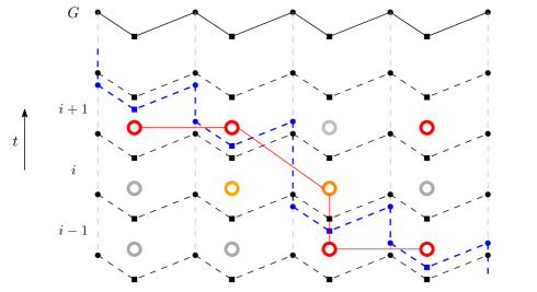
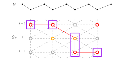
(a) The discrepancy sequence projected onto $\tilde{G}_{F}$.

(b) An open path in the site percolation on $\tilde{G}_{F}$

Figure 1. Discrepancy sequence and site percolation

Recall that $i(t)=\lfloor t/k\rfloor$ is the time interval $t$ belongs to. Naturally, we would like our path $\gamma$ to pass through sites $\{(a_{-\ell},i(t_{-\ell}))\}_{0\leq\ell\leq L}$, where the updates in $\zeta^{\circ}$ take place, and stays at each hyperedge until the next update happens at a nearby hyperedge. Let $\gamma_{\ell}$ denote the segment of $\gamma$ corresponding to the $\ell$’th update $(\nu_{{-\ell}},a_{-\ell},t_{-\ell})$ of $\zeta^{\circ}$. If the next (i.e., $(\ell-1)$’th) update happens at the same time interval as the $\ell$’th update, i.e., $i(t_{-\ell})=i(t_{-\ell+1})$, then we define $\gamma_{\ell}$ to be a singleton pair $((a_{-\ell},i(t_{-\ell})))$. Otherwise if $i(t_{-\ell})<i(t_{-\ell+1})$, we define $\gamma_{\ell}$ as the vertical line

$$\gamma_{\ell}\equiv\gamma_{\ell}(\zeta^{\circ})\equiv\left((a_{-\ell},j):i(t_{-\ell})\leq j<i(t_{-\ell+1})\right).$$

Let $\gamma\equiv\cup_{0\leq\ell\leq L}\gamma_{\ell}$ be the sequential concatenation of $(\gamma_{\ell})_{0\leq\ell\leq L}$. It is easy to observe that each $\gamma_{\ell}$ is a connected path in $\tilde{G}_{F}$, $\gamma_{0}$ intersects $F\times\{M\}$ at $(a_{0},i(t_{1})-1)=(a_{0},M)$, and $\gamma_{L}$ intersects $F\times\{0\}$ at $(a_{-L},0)$. To verify the rest of the requirements of Lemma 3.3, we first check that every site $(a,i)\in\gamma$ is bad, distinguishing three cases:

1. For $0\leq\ell\leq L$, if $\gamma_{\ell}$ is a singleton, then it must have the form $\gamma_{\ell}=\{(a,i)=(a_{-\ell},i(t_{-\ell}))\}$. By condition (4) $Y_{t_{-\ell}}(\partial a_{-\ell})=\underline{1}$ and hence also $Y_{T_{i-1},t_{-\ell}}(\partial a_{-\ell})=\underline{1}$, implying that $(a,i)$ is indeed active.

2. For $0\leq\ell<L$, if $\gamma_{\ell}$ consists of more than one site, then arguing as above we know that the first site $(a_{-\ell},i(t_{-\ell}))$ is active. For each of the remaining sites $(a,i)$ with $i(t_{-\ell})<i<i(t_{-(\ell-1)})$, rewriting the assumption gives

   $$t_{-\ell}<T_{i}<T_{i+1}\leq t_{-(\ell-1)},$$

   i.e., $v_{-\ell}\in\partial a_{-\ell}$ is not updated during the time interval ${[}T_{i},T_{i+1})$ and so $(a_{-\ell},i)\in\gamma_{\ell}$ is susceptible. Following the second case of Definition 3.2, $(a_{-\ell},i)$ is bad for all $i(t_{-\ell})<i<i(t_{-(\ell-1)})$.

3. For each $(a_{-L},i)\in\gamma_{L}$, recall from the definition of $\zeta^{\circ}$ that $a_{-L}=a_{-(L-1)}$ and that $t_{-}(v_{-L},t_{-(L-1)})=0$, i.e., $v_{-L}$ is never updated before $T_{i(t_{-(L-1)})}$. Hence all sites $(a_{-L},i)$ with $i<i(t_{-(L-1)})$ are susceptible. Their badness then follows from the fact that $(a_{-L},0)$ is bad (recall that $(a,0)$ is defined to be active for all $a\in F$).

All that is left is to check that $\gamma_{\ell}$ is connected to $\gamma_{\ell-1}$ for each $1\leq\ell\leq L$. The connectivity of $\gamma_{L}$ to $\gamma_{L-1}$ is trivial. For $1\leq\ell<L$, the first site in $\gamma_{\ell-1}$ is $(a_{-(\ell-1)},i^{\textup{start}}_{\ell-1}\equiv i(t_{-(\ell-1)}))$ and the last site in $\gamma_{\ell}$ is $(a_{-\ell},i^{\textup{end}}_{\ell})$ with

$$i^{\textup{end}}_{\ell}\equiv\begin{cases}i(t_{-(\ell-1)})-1&\textup{if }i(t_{-(\ell-1)})>i(t_{-\ell}),\\ i(t_{-\ell})&\textup{if }i(t_{-(\ell-1)})=i(t_{-\ell})\end{cases}.$$

In either case, site $(a_{-\ell},i^{\textup{end}}_{\ell})$ is connected to $(a_{-(\ell-1)},i^{\textup{start}}_{\ell-1})$ in $\tilde{G}_{F}$ since $\partial a_{-\ell}\cap\partial a_{-(\ell-1)}\supseteq\{v_{-\ell}\}\neq\varnothing$ and

$$i^{\textup{start}}_{\ell-1}-i^{\textup{end}}_{\ell}=1-\mathbf{1}\{i(t_{-(\ell-1)})=i(t_{-\ell})\}\in\{0,1\}.$$

∎

3.2. Proof of Theorem 3.1

By Proposition 2.1 and (2), we aim to show that under the assumptions of Theorems 3.1, there exists some constant $C$ such that for $M\equiv\lceil C\log n\rceil$, $\mathbb{P}[t_{\mathrm{coup}}>T_{M+1}]\leq 1/8$. In fact, as will be clear from the proof, once we find an $M$ for which our analysis yields that $\mathbb{P}[t_{\mathrm{coup}}>T_{M+1}]\leq 1/8$, doubling it gives $\mathbb{P}[t_{\mathrm{coup}}>T_{2(M+1)}]\leq O(n^{-1})$.

Using Lemma 3.3, it suffices to bound the probability that there exists an oriented path from $F\times\{0\}$ consisting of bad sites. We begin with some basic properties of the auxiliary percolation process.

Proposition 3.4.

Let $\mathsf{A}(a,i)$ (resp. $\mathsf{S}(a,i)$) be the event that site $(a,i)$ is active (resp. susceptible). Then for every distinct $(a,i),(b,j)\in\tilde{G}_{F}$ with $i\geq j\geq 1$,

$$\mathbb{P}(\mathsf{A}(a,i))\leq(k^{2}+1)2^{-k}+ke^{-k},\quad\mathbb{P}(\mathsf{S}(a,i+1))\leq ke^{-k}$$ (6)

$$\mathbb{P}(\mathsf{A}(a,i)\mid\mathsf{A}(b,j))\leq(k^{2}+1)2^{-k+|\partial a\cap\partial b|}+ke^{-k},$$ (7)

Moreover for every set of sites $S$ in $\tilde{G}_{F}$, if for all $(b,j)\in S$, $(a,i)$ and $(b,j)$ are not connected in $\tilde{E}_{F}$, then $\mathsf{A}(a,i),\mathsf{S}(a,i)$ are independent of the events $\{\mathsf{A}(b,j),\mathsf{S}(b,j):(b,j)\in S\}$.

Proof.

The second part of (6) is simply a union bound. To show the first part of (6), we notice that if $\mathsf{A}(a,i)$ happens then so does one of the following scenarios

• Some $v\in\partial a$ is not updated in ${[}T_{i-1},T_{i})$, namely $\mathsf{S}(a,i-1)$ happens.

• Case (a) fails but $a$ gets $T_{i-1}$-activated at some time $s\in{[}T_{i},T_{i+1})$.

Case (a) happens with probability at most $ke^{-k}$. Conditioned on the failure of case (a), namely every $v\in\partial a$ being updated in $[T_{i-1},T_{i})$, $(Y_{T_{i-1},s}(u))_{u\in\partial a}$ become $\mathrm{i.i.d.}$ Bernoulli($1/2$) r.v.’s for all $T_{i}\leq s<T_{i+1}$. For case (b) to happen, there must exist $u\in\partial a$ and $s\in{[}T_{i},T_{i+1})$ such that $(u,s,1)\in\xi$ and $Y_{T_{i-1},s}(\partial a)=\underline{1}$. Hence conditioned on the failure of case $a$, by Markov’s inequality the probability of case (b) is at most $k^{2}2^{-k}$, where the term $k^{2}$ represents the expected number of updates of the vertices in $\partial a$ during ${[}T_{i},T_{i+1})$ and $2^{-k}$ is the probability that $Y_{T_{i-1},s}(\partial a)=\underline{1}$ at the time of update. Combining the two cases gives the first half of (6). The proof of (7) is completely analogous, where the only difference is that we first argue that

$$\mathbb{P}(\mathsf{A}(a,i)\mid\mathsf{A}(b,j))\leq\mathbb{P}(\mathsf{A}(a,i)\mid Y_{T_{i-1},s}(\partial a\cap\partial b)=\underline{1}\text{ for all }s\in{[}T_{i},T_{i+1})).$$

and then apply the same reasoning as before to $\partial a\setminus\partial b$.

Finally, note that the events $\mathsf{A}(a,i)$ and $\mathsf{S}(a,i)$ depend on $\xi$ only through $\partial a\times(T_{i-1},T_{i+1})$. Hence the independency result follows from the independency of Poisson point process. ∎

In order to perform a first moment calculation in an efficient manner we restrict our attention to a special type of path.

Definition 3.5.

We say that an oriented path $((a_{0},i_{0}),(a_{1},i_{1}),\ldots,(a_{r},i_{r}))$ in $\tilde{G}_{F}$ is a minimal path if $i_{0}=0$, $i_{1}=1$ and for all $j_{1}\leq r-2$ and $j_{2}\in[j_{1}+2,r]$ we have that $((a_{j_{1}},i_{j_{1}}),(a_{j_{2}},i_{j_{2}}))\notin\tilde{E}_{F}$. Let $\Gamma_{\mathrm{min},r}$ be the collection of all minimal paths of length $r$.

Here we require $i_{1}=1$ because we are primarily interested in upperbounding the number of open paths connecting $F\times\{0\}$ to $F\times{M}$ for some $M\geq 1$ and additonal steps within $F\times\{0\}$ will not help. Observe that every oriented path in $\tilde{G}_{F}$ can be transformed into a minimal path by deleting some vertices from it.

Proof of Theorem 3.1, Part 1.

Fix $M\equiv\lceil C\log n\rceil$ where the constant $C$ shall be determined later. Note that by Lemma 3.3, if $t_{\mathrm{coup}}>T_{M+1}$, then there must be some minimal path

$$\gamma_{M}=((a_{0},i_{0}),(a_{1},i_{1}),\ldots,(a_{M},i_{M}))\in\Gamma_{\min,M}$$

consisting of bad sites. We now estimate the expected number of such paths. For brevity, we call a minimal path $\gamma$ bad if every site of $\gamma$ is bad.

Using the notations of Proposition 3.4, for every $\gamma\in\Gamma_{\min,2r}$, we can write

$$\mathbb{E}[\mathbf{1}\{\gamma\textup{ is bad}\}]\leq\mathbb{P}\Big{(}\bigcap_{\ell=0}^{2r}(\mathsf{A}(a_{\ell},i_{\ell})\cup\mathsf{S}(a_{\ell},i_{\ell}))\Big{)}\leq\mathbb{P}\Big{(}\bigcap_{\ell=1}^{r}(\mathsf{A}(a_{2\ell},i_{2\ell})\cup\mathsf{S}(a_{2\ell},i_{2\ell}))\Big{)},$$

where in the last step we discard all odd events in order to obtain the desirable independence. Indeed, by the definition of a minimal path, for all $j<\ell$, $(a_{2\ell},i_{2\ell})$ is not connected to $(a_{2j},i_{2j})$. Hence by Proposition 3.4, the events $\{\mathsf{A}(a_{2\ell},i_{2\ell})\cup\mathsf{S}(a_{2\ell},i_{2\ell})\}_{1\leq\ell\leq r}$ are mutually independent and

$$\mathbb{E}[\mathbf{1}\{\gamma\textup{ is bad}\}]\leq\prod_{\ell=1}^{r}\big{[}(k^{2}+1)2^{-k}+2ke^{-k}\big{]}\leq\big{(}2k^{2}2^{-k}\big{)}^{r}$$ (8)

To conclude the proof we note that

$$|\Gamma_{\mathrm{min},2r}|\leq n(2k(\Delta-1)+1)^{2r}\leq(4k^{2}\Delta^{2})^{r}n,$$ (9)

where the term $n$ accounts for the choice of the initial site of the path. By the above analysis the expected number of paths in $\Gamma_{\mathrm{min},2r}$ consisting of bad sites is at most $(4k^{2}\Delta^{2}\times 2k^{2}2^{-k})^{r}n$. By our assumption that $\Delta<2^{k/2}/(\sqrt{8}k^{2})$, we get that there exists some constant $C$ such that for $r=\lceil C\log n\rceil$ the last expectation is at most $1/8$. This concludes the proof of part 1 of Theorem 3.1. ∎

We now explain the necessary adaptations for the proof of part 2. In the new setup if $a\neq b$ and $\partial a\cap\partial b\neq\varnothing$, then $|\partial a\cap\partial b|=1$. Thus the event that $(a,i)$ is bad barely affects the probability that $(b,j)$ is bad (for $a\neq b$). However, it is more challenging to control the conditional probability that $(a,i+1)$ is bad, given that $(a,i)$ is bad. To overcome this difficulty we modify the underlying graph $\tilde{G}_{F}$ slightly.

Definition 3.6.

Let $\bar{G}_{F}$ be an oriented graph with vertex-set $F\times\mathbb{N}$ and edge-set $\bar{E}_{F}$ satisfying that for every pairs of hyperedges $a,b\in F$ and integers $i,j\in\mathbb{N}$, there is an (oriented) edge from site $(a,i)$ to site $(b,j)$ in $\bar{E}_{F}$ if and only if $a=b$ and $j=i+2$ or $a\neq b$ and

$$\partial a\cap\partial b\neq\varnothing\textup{ and }j-i\in\{0,1,2\}.$$ (10)

We say that an oriented path $((a_{0},i_{0}),(a_{1},i_{1}),\ldots,(a_{r},i_{r}))$ in $\bar{G}_{F}$ is a minimal path if $i_{0}=1$, $i_{1}>1$ and for all $j_{1}\leq r-2$ and $j_{2}\in[j_{1}+2,r]$ we have that $((a_{j_{1}},i_{j_{1}}),(a_{j_{2}},i_{j_{2}}))\notin\bar{E}_{F}$. Let $\bar{\Gamma}_{\mathrm{min},r}$ be the collection of all minimal paths of length $r$ in $\bar{G}_{F}$.

Observe that every path $\gamma$ in $\tilde{G}_{F}$ can be transformed into a path in $\bar{G}_{F}$ by deleting some of its vertices. Namely, whenever we have two consecutive steps in $\gamma$ such that $((a_{\ell},i_{\ell}),(a_{\ell+1},i_{\ell+1}))\in\tilde{E}_{F}\setminus\bar{E}_{F}$, it must satisfy that $(a_{\ell+1},i_{\ell+1})=(a_{\ell},i_{\ell}+1)$ and one can check that in this case $((a_{\ell},i_{\ell}),(a_{\ell+2},i_{\ell+2}))\in\bar{G}_{F}$. By repeatedly deleting $(a_{\ell+1},i_{\ell+1})$ from $\gamma$, where $\ell$ is the minimal index such that $(a_{\ell+1},i_{\ell+1})=(a_{\ell},i_{\ell}+1)$ and $(a_{\ell},i_{\ell})$ has not been deleted already, we obtain a path in $\bar{G}_{F}$. From there, one can further take a subpath such that it is a minimal path in $\bar{G}_{F}$.

Proof of Theorem 3.1, Part 2.

As before, if $t_{\mathrm{coup}}>T_{2(M+1)}$, then there must be some minimal path $((a_{0},i_{0}),(a_{1},i_{1}),\ldots,(a_{M},i_{M}))$ in $\bar{G}_{F}$ consisting of bad sites. We argue that the conditional probability that $(a_{\ell},i_{\ell})$ is bad, given that $(a_{0},i_{0}),(a_{1},i_{1}),\ldots(a_{\ell-1},i_{\ell-1})$ are all bad, is at most

$$(1+k^{2})2^{-(k-1)}+2ke^{-k}\leq 3k^{2}2^{-k}\quad\textup{(for $k>2$)}.$$

Indeed, by the linearity assumption we have that either $(a_{\ell-1},i_{\ell-1})=(a_{\ell},i_{\ell}-2)$ or $|\partial a_{\ell-1}\cap\partial a_{\ell}|=1$. In the first case, the same independency argument as before shows that the conditional probability that $(a_{\ell},i_{\ell})$ is also bad is at most $(1+k^{2})2^{-k}+2e^{-k}$. For the second case, $(a_{\ell},i_{\ell})$ must be active and the desired bound follows from (7).

As before, we conclude by noting that $|\bar{\Gamma}_{\mathrm{min},r}|\leq n(3k(\Delta-1)+1)^{r}\leq(3k\Delta)^{r}n$ and so the expected number of paths in $\bar{\Gamma}_{\mathrm{min},r}$ consisting of bad sites is at most

$$(3k\Delta\times 3k^{2}2^{-k})^{r}n=(9k^{3}\Delta 2^{-k})^{r}n\leq 1/8\color[rgb]{0,0,0},$$

provided that $r\geq C\log n$. ∎

4. General Hypergraphs

4.1. Minimal path

In this subsection we give the general setup for Theorem 1.1 and 1.3. The first improvement from Section 3 is based on the observation that although it takes time $k$ to update all vertices of a hyperedge at least once with high probability, on average it only takes $O(1)$ time to update each vertex. This motivates us to study the propagation of discrepancies on both vertices and hyperedges in continuous time.

Recall the definition of activation from Definition 2.4. Observe that, in order for a discrepancy to propagate from an active hyperedge to a nearby hyperedge, the latter hyperedge must be activated before every vertex in their intersection is updated at least once, erasing all possible dependence. Thus we define the following continuous time analog of the time block from the previous section.

Definition 4.1.

For each $v\in V$, $t\geq 0$, we define the deactivation time of $v$ (after time $t$) as the first time $v$ is updated after time $t$, namely,

$$T_{+}(v;t)\equiv\inf\left\{s>t:(v,s,1)\in\xi\text{ or }(v,s,0)\in\xi\right\},$$

For each $a,b\in F$ and $t\geq 0$, we define the relative deactivation time of $a$ w.r.t. $b$ (after time $t$) as the first time $s>t$ such that every vertex in the intersection $\partial a\cap\partial b$ is updated at least once by time $s$, namely,

$$T_{+}(a;b,t)\equiv\max_{v\in\partial a}T_{+}(v;b,t),\quad\textup{ where }T_{+}(v;b,t)\equiv\begin{cases}T_{+}(v;t)&v\in\partial b,\\ t&v\notin\partial b\end{cases}.$$

In particular, the deactivation time of $a$ is $T_{+}(a;t)\equiv T_{+}(a;a,t)=\max_{v\in\partial a}T_{+}(v;t)$.

Under the definition above, discrepancies can only pass from one hyperedge to another before the first hyperedge is relatively deactivated w.r.t. the latter hyperedge. In other word, (relative) deactivation time gives the time window of discrepancy propagation.

Let $\tilde{G}$ be the Cartesian product of $G$ and the time interval ${[}0,\infty)$. Namely for two sites $(w_{1},t_{1}),(w_{2},t_{2})\in\tilde{V}\equiv(V\cup F)\times{[}0,\infty)$, there exists an (oriented) edge connecting $(w_{1},t_{1})$ to $(w_{2},t_{2})$ in $\tilde{G}$ if and only if

$$w_{1}=w_{2},\ t_{1}\leq t_{2}\color[rgb]{0,0,0}\quad\textup{or}\quad w_{1}\in\partial w_{2},\ t_{1}=t_{2}.$$

The set $\tilde{G}$ can be viewed as the continuous version of the space-time slab.

Definition 4.2.

Given a sequence $\gamma_{L}\equiv\{(v_{\ell},a_{\ell},t_{\ell})\}_{0\leq\ell\leq L}$, we say that $\gamma_{L}$ is a path of length $L$ in $\tilde{G}$ if $t_{0}=0$, $v_{0}\in\partial a_{0},a_{0}=a_{1}$ and for each $1\leq\ell\leq L$ we have that $t_{\ell-1}<t_{\ell}$, $v_{\ell}\in\partial a_{\ell}$ and $\partial a_{\ell-1}\cap\partial a_{\ell}\neq\varnothing$. We further say that $\gamma_{L}$ is a path up to time $t$ to indicate that $t_{L}<t$. Let $\Gamma_{L}$ denote the set of paths of length $L$ and $\Gamma_{L}(t)$ denote the subset of paths up to time $t$.

In the previous section, we defined an auxiliary percolation on the discrete space-time slab such that every discrepancy sequence can be projected onto an open path in the percolation. Without a good analog of the percolation in continuous time, we look at the analog of “open paths” directly, i.e., paths of $\Gamma_{L}(t)$ that can be interpreted as the projections of discrepancy sequences.

Definition 4.3.

Fix an update sequence $\xi$ and a path $\gamma_{L}=\{(v_{\ell},a_{\ell},t_{\ell})_{0\leq\ell\leq L}\}\in\Gamma_{L}$. For each $1\leq\ell\leq L$, we say that $(v_{\ell},a_{\ell},t_{\ell})$, the $\ell$th step of $\gamma_{L}$, is a minimal step of $\gamma_{L}$ if all of the following six events hold:

$$\mathsf{A}_{\ell}\equiv\{(v_{\ell},t_{\ell},1)\in\xi\},\qquad\qquad\qquad\quad\ \,\mathsf{B}_{\ell}\equiv\{t_{\ell}\leq T_{+}(a_{\ell};a_{\ell-1},t_{\ell-1})\},\quad$$

$$\mathsf{C}_{\ell}\equiv\begin{cases}\{t_{\ell}>T_{+}(a_{\ell};a_{\ell},0)\}\cap(\cap_{r=1}^{\ell-2}\{t_{\ell}>T_{+}(a_{\ell};a_{r},t_{r})\})&\ell\geq 2\\ \varnothing^{c}&\ell=1\\ \end{cases},$$

$$\mathsf{D}^{1}_{\ell}\equiv\{Y_{t_{\ell}}((\partial a_{\ell}\cap\partial a^{c}_{\ell-1})\setminus\{v_{\ell}\})=\underline{1}\},\quad\mathsf{D}^{2}_{\ell}\equiv\{Y_{t_{\ell}}((\partial a_{\ell}\cap\partial a_{\ell-1})\setminus\{v_{\ell}\})=\underline{1}\},$$ (11)

$$\mathsf{E}_{\ell}\equiv\begin{cases}\{Y_{t_{\ell}}(\partial a_{\ell-1}\setminus\partial a_{\ell})\neq\underline{1}\}&v_{\ell}\in\partial a_{\ell-1}\cap\partial a_{\ell},a_{\ell-1}\neq a_{\ell}\\ \varnothing^{c}&\textup{otherwise}\end{cases}.$$

We say that $\gamma_{L}$ is a minimal path if $(v_{\ell},a_{\ell},t_{\ell})$ is a minimal step, for each $1\leq\ell\leq L$. We further say that $\gamma_{L}$ is a minimal path up to time $t$, if it is a minimal path and $t_{L}<t\leq T_{+}(v_{L};t_{L})$. Let $\Gamma_{\min,L}$ be the set of minimal paths of length $L$. Similarly, we define $\Gamma_{\min,L}(t)\equiv\{\gamma_{L}\in\Gamma_{\min,L}:\gamma_{L}\text{ is a minimal path up to time }t\}$. We note that both $\Gamma_{\min,L}$ and $\Gamma_{\min,L}(t)$ depend on the update sequence $\xi$.

Remark 4.4.

The six events above can be roughly explained as the following:

1. $\mathsf{A}_{\ell}$: There is an update to $1$ at vertex $v_{\ell}$ at time $t_{\ell}$.

2. $\mathsf{B}_{\ell}$: At time $t_{\ell}$, $a_{\ell}$ has not been deactivated from the step immedaitely before it (i.e., the activation of $a_{\ell-1}$ at time $t_{\ell-1}$).

3. $\mathsf{C}_{\ell}$: At time $t_{\ell}$, $a_{\ell}$ has been deactivated from all steps at least two steps ago (i.e., the activations of $a_{r}$ at time $t_{r}$ for $r\leq\ell-2$).

4. $\mathsf{D}^{1}_{\ell}\cap\mathsf{D}^{2}_{\ell}$: At time $t_{\ell}$, the configuration on $\partial a_{\ell}\setminus\{v_{\ell}\}$ is all $1$. Thus update at $v_{\ell}$ is prone to be blocked by $a_{\ell}$. Here we differentiate $\mathsf{D}^{1}_{\ell}$ and $\mathsf{D}^{2}_{\ell}$ because the conditional distribution of $Y_{t_{\ell}}$ on $\partial a_{\ell}\cap a_{\ell-1}$ and $\partial a_{\ell}\cap a_{\ell-1}^{c}$ are very different and are easier to be analysed separately.

5. $\mathsf{E}_{\ell}$: If consider the $\ell$’th step being $(v_{\ell},a_{\ell-1},t_{\ell})$ instead of $(v_{\ell},a_{\ell},t_{\ell})$, then the new tuple $(v_{\ell},a_{\ell-1},t_{\ell})$ does not satisfy the first five events because it violates $\mathsf{D}^{2}_{\ell}$. This requirement ensures that we stay at the same hyperedge whenever possible.

In the definition above, event $\mathsf{A}_{\ell}\cap\mathsf{D}^{1}_{\ell}\cap\mathsf{D}^{2}_{\ell}$ guarrantees that $(v_{\ell},a_{\ell})$ is activated at time $t_{\ell}$. The event $\mathsf{B}_{\ell}$ guarrantees that $a_{\ell}$ has not been deactivated w.r.t. $a_{\ell-1}$ after time $t_{\ell-1}$. Together, events $\{\mathsf{A}_{\ell},\mathsf{B}_{\ell},\mathsf{D}^{1}_{\ell},\mathsf{D}^{2}_{\ell}\}_{1\leq\ell\leq L}$ imply that $\gamma_{L}$ can potentially be the projection of some discrepancy sequence $\zeta$ (as will be proved in the lemma below).

Further, the events $\{\mathsf{C}_{\ell}\}_{1\leq\ell\leq L}$ imply that no subpath of $\gamma_{L}$ satisfies the same condition while $\{\mathsf{E}_{\ell}\}_{1\leq\ell\leq L}$ further require paths to stay at the same hyperedge whenever possible (this requirement is imposed to obtain a better control on the number of minimal paths), justifying the name “minimal”.

Lemma 4.5.

For each update sequence $\xi$, if $t_{\textup{coup}}>T$, then there exists a constant $L\geq 0$ and a minimal path $\gamma_{L}=((v_{\ell},a_{\ell},t_{\ell}))_{0\leq\ell\leq L}\in\Gamma_{\min,L}(T)$.

Proof.

Recall the construction of a discrepancy sequence $\zeta=\zeta(\xi)=((u_{i},b_{i},s_{i}))_{0\leq i\leq M}$ (here we use the representation moving forward in time, with $(b_{0},s_{0})=(b_{1},0)$). It satisfies for all $1\leq i\leq M$, that (a) $u_{i-1},u_{i}\in\partial b_{i}$, (b) $(u_{i},s_{i},1)\in\xi$, (c) $Y_{s_{i}}(b_{i})=\underline{1}$ and (d)

$$s_{i-1}<s_{i}\leq T_{+}(u_{i-1};s_{i-1}),\quad\text{hence in particular,}\quad s_{i-1}<s_{i}\leq T_{+}(b_{i};b_{i-1},s_{i-1}).$$ (12)

One can construct a minimal path based on $\zeta$ as follows:

1. Let $\gamma^{1}\equiv((v^{1}_{\ell},a^{1}_{\ell},t^{1}_{\ell}))_{0\leq\ell\leq 1}\equiv((u_{\ell},b_{\ell},s_{\ell}))_{0\leq\ell\leq 1}$. It follows from the construction of a discrepancy sequence, in particular from the fact that $b_{0}=b_{1}$, that $\gamma^{1}$ is a minimal path of length $L_{1}\equiv 1$ up to time $s_{2}$.

2. For $2\leq i\leq M$, suppose we have already constructed $\gamma^{i-1}=((v^{i-1}_{\ell},a^{i-1}_{\ell},t^{i-1}_{\ell}))_{0\leq\ell\leq L_{i-1}}\in\Gamma_{\min,L_{i-1}}(s_{i})$ with $L_{i-1}\leq i-1$ and

   $$(v^{i-1}_{L_{i-1}},t^{i-1}_{L_{i-1}})=(u_{i-1},t_{i-1}).$$ (13)

   To construct $\gamma^{i}$, let

   $$\ell_{\star}\equiv\ell_{\star}(i)\equiv\begin{cases}0&s_{i}\leq T_{+}(b_{i};b_{i},0)\\ \min_{1\leq\ell\leq L_{i-1}}\{\ell:s_{i}\leq T_{+}(b_{i};a^{i-1}_{\ell},t^{i-1}_{\ell})\}&\textup{otherwise}\end{cases}.$$

   Note that $\ell_{\star}$ is well-defined since by (12) and (13), the condition $\{\ell:s_{i}\leq T_{+}(b_{i};a^{i-1}_{\ell},t^{i-1}_{\ell})\}$ is satisfied by $\ell=L_{i-1}$. If $\ell_{\star}=0$, then there exists $v_{\star}\in\partial b_{i}$ such that $s_{i}\leq T_{+}(v_{\star};0)$. In this case, we define $L_{i}=1$ and

   $$\gamma^{i}\equiv((v^{i}_{\ell},a^{i}_{\ell},t^{i}_{\ell}))_{0\leq\ell\leq 1}\equiv((v_{\star},b_{i},0),(u_{i},b_{i},s_{i})).$$

   Otherwise, we define $L_{i}=\ell_{\star}+1$, $(v^{i}_{\ell},a^{i}_{\ell},t^{i}_{\ell})\equiv(v^{i-1}_{\ell},a^{i-1}_{\ell},t^{i-1}_{\ell}),0\leq\ell\leq\ell_{\star}$ and

   $$(v^{i}_{L_{i}},a^{i}_{L_{i}},t^{i}_{L_{i}})\equiv\begin{cases}(u_{i},a^{i-1}_{\ell_{\star}},s_{i})&\textup{if }u_{i}\in\partial a^{i-1}_{\ell_{\star}}\textup{ and $Y_{s_{i}}(\partial a^{i-1}_{\ell_{\star}})=\underline{1}$,}\\ (u_{i},b_{i},s_{i})&\textup{otherwise.}\end{cases}$$ (14)

   In either case, one can check that the six events defined in (11) are satisfied for $\ell=L_{i}$ and hence $(v^{i}_{L_{i}},a^{i}_{L_{i}},t^{i}_{L_{i}})$ is a minimal step of $\gamma^{i}$. Indeed, the occurrence of $\mathsf{A}_{L_{i}},\mathsf{B}_{L_{i}},\mathsf{D}^{1}_{L_{i}},\mathsf{D}^{2}_{L_{i}}$ follows from the construction of a discrepancy sequence, the occurrence of $\mathsf{C}_{L_{i}}$ follows from the minimality of $\ell_{\star}$ and that of $\mathsf{E}_{L_{i}}$ follows from (14). By construction, $((v^{i}_{r},a^{i}_{r},t^{i}_{r}))_{0\leq\ell\leq L_{i}-1}$ is a subpath of $\gamma^{i-1}\in\Gamma_{\min,L_{i-1}}(s_{i})$ and hence is minimal path itself. Therefore $\gamma^{i}$ is a minimal path of length $L_{i}$ up to $s_{i+1}$.

To conclude the proof, one can take $\gamma^{M}$ and note that $T_{+}(v_{L_{M}}^{M};t_{L_{M}}^{M})=T_{+}(u_{M};s_{M})\geq T$ by the definition of $\zeta$. ∎

Remark 4.6.

We will use $\Gamma_{\textup{proj},L}\subset\Gamma_{\min,L}$ to denote the set of minimal paths that are projected from some discrepancy sequences as in the proof above.

Lemma 4.5 implies that for every time $T\geq 0$ and integer $L\geq 1$,

$$\mathbb{P}(t_{\textup{coup}}\geq T) \leq\mathbb{P}(\Gamma_{\textup{proj},L-1}(T)\neq\varnothing)+\mathbb{P}(\Gamma_{\textup{proj},L}\neq\varnothing)$$ (15)

$$\leq\mathbb{P}(\Gamma_{\textup{proj},L-1}(T)\neq\varnothing)+\mathbb{P}(\Gamma_{\min,L}\neq\varnothing).$$ (16)

The next lemma bounds the first term on the right hand side.

Lemma 4.7.

Let $T\in\mathbb{N}$. Denote $L=\lfloor cT\rfloor$, where $c=\frac{1}{4\log(2k^{2}\Delta)}$. Then

$$\mathbb{P}(\Gamma_{\textup{proj},L-1}(T)\neq\varnothing)\leq n\exp(-T/4).$$

Proof.

Consider constructing a path in $\Gamma_{\textup{proj},L-1}(T)$ by first choosing the locations of “jumps” and then picking their times. The number of ways of choosing a sequence $\underline{w}\equiv(a_{\ell})_{0\leq\ell\leq L-1}$ such that $\partial a_{\ell}\cap\partial a_{\ell-1}\neq\varnothing$ for all $1\leq\ell\leq L-1$, is at most $n(\Delta k)^{L}$. For each fixed $\underline{w}$, recursively define $T_{0}\equiv 0$ and $T_{\ell+1}\equiv T_{+}(a_{\ell+1};a_{\ell},T_{\ell})$ for $0\leq\ell\leq L-2$. If there exists a sequences of times $\underline{s}\equiv(s_{\ell})_{0\leq\ell\leq L-1}$ and vertices $\underline{v}\equiv(v_{\ell})_{0\leq\ell\leq L-1}$ such that the path $\gamma_{L-1}\equiv((v_{\ell},a_{\ell},s_{\ell}))_{0\leq\ell\leq L-1}$ is a minimal path up to time $T$, then $s_{0}=T_{0}=0$, and one can show inductively that

$$s_{\ell}\leq T_{+}(a_{\ell};a_{\ell-1},s_{\ell-1})\leq T_{+}(a_{\ell};a_{\ell-1},T_{\ell-1})=T_{\ell},$$

using the induction step ($s_{\ell-1}\leq T_{\ell-1}$) and the monotonicity of $T_{+}(a;b,t)$ in $t$. The existence of $\underline{s}$ further implies that

$$T_{L}\equiv T_{+}(a_{L-1};a_{L-1},T_{L-1})\geq T_{+}(v_{L-1};s_{L-1})\geq T.$$

By construction, the joint law of $(T_{\ell}-T_{\ell-1})_{0\leq\ell\leq L}$ is stochastically dominated by that of $(Z_{\ell})_{0\leq\ell\leq L}$ where $Z_{\ell}:=\max(Z_{\ell,1},\ldots,Z_{\ell,k})$ and $(Z_{\ell,i})_{1\leq i\leq k,1\leq\ell\leq L}$ are i.i.d. exponential random variables with rate $1$. Note that using the order statistic of $Z_{\ell,1},\ldots,Z_{\ell,k}$, we can decompose $Z_{\ell}$ into a sum $\sum_{i=1}^{k}J_{\ell,i}$ of independent exponential r.v.’s with $\mathbb{E}[J_{\ell,i}]=i^{-1}$. Hence for all $\lambda\in(0,1/2)$ and $\ell\leq L$,

$$\mathbb{E}[e^{\lambda Z_{\ell}}]=\prod_{i=1}^{k}\mathbb{E}[e^{\lambda J_{\ell,i}}]=\prod_{i=1}^{k}\Big{(}1+\frac{\lambda}{i-\lambda}\Big{)}\leq\prod_{i=1}^{k}\Big{(}1+\frac{1}{i}\Big{)}\leq 2e^{\frac{1}{2}+\cdots+\frac{1}{k}}\leq e^{\log(2k)}.$$

By Markov’s inequality, independence of $Z_{\ell}$’s and the aforementioned stochastic domination,

$$\mathbb{P}(T_{L}\geq T)\leq\mathbb{E}[e^{(T_{L}-T)/2}]=e^{-T/2}e^{L\log(2k)}\leq e^{-[1-2c\log(2k)]T/2}.$$

Therefore by the arguments above together with the choice $c=\frac{1}{4\log(2k^{2}\Delta)}$,

$$\mathbb{P}(\Gamma_{\textup{proj},L-1}(T)\neq\varnothing)\leq n(\Delta k)^{cT}\mathbb{P}(T_{L}\geq T)\leq n(\Delta k)^{cT}e^{-[1-2c\log(2k)]T/2}=ne^{-T/4},$$

as desired. ∎

4.2. Redacted path

In the remainder of the section, we bound the size of $\Gamma_{\min,L}$. Our basic approach is to bound for each $\gamma_{L}\in\Gamma_{\min,L}$ the expected number of ways to extend $\gamma_{L}$ by two steps. However, the “vanilla-version” of this expectation can be much bigger than 1. Intuitively, for general hypergraphs, hyperedges may be highly overlapping with each other. Thus when one hyperedge is all $1$ in process $Y_{t}$, its neighbouring hyperedges may also be all $1$ with little extra cost. This phenomenon leads to numerous local “tangles” where multiple choices of the immediate next step exist for the same second-next step, blowing up the number of extensions significantly.

To overcome the aforementioned obstacle, we divide the steps of a minimal path into good branchings (i.e., small overlaps) and bad branchings (i.e., large overlaps) and skip the “tangles” by ignoring the first step of a bad branching and recording only the “key” step instead. More precisely, given a path $\gamma_{L}=\{(u_{\ell},b_{\ell},s_{\ell})\}_{0\leq\ell\leq L}\in\Gamma_{L}$, we classify each of the steps $1\leq\ell\leq L$ into one of the following three cases: (see also Figure 2)

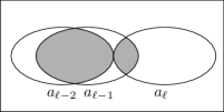
Figure 2. Good/Type-I/Type-II branching in redacted paths

1. We say that $(v_{\ell},a_{\ell},t_{\ell})$ is a good branching if $|\partial a_{\ell-1}\cap\partial a_{\ell}|\leq k/3$.

2. We say that $\{(v_{\ell-1},a_{\ell-1},t_{\ell-1}),(v_{\ell},a_{\ell},t_{\ell})\}$ is a type-I (bad) branching if

   $$|\partial a_{\ell-2}\cap\partial a_{\ell-1}|>k/3,\quad\partial a_{\ell-2}\cap\partial a_{\ell}=\varnothing.$$

3. We say that $\{(v_{\ell-1},a_{\ell-1},t_{\ell-1}),(v_{\ell},a_{\ell},t_{\ell})\}$ is a type-II (bad) branching if

   $$|\partial a_{\ell-2}\cap\partial a_{\ell-1}|>k/3,\quad\partial a_{\ell-2}\cap\partial a_{\ell}\neq\varnothing.$$

For each $\gamma_{L}=((v_{\ell},a_{\ell},t_{\ell}))_{0\leq\ell\leq L}\in\Gamma_{L}$, we use the following greedy algorithm to partition $\gamma_{L}$ into disjoint segments of size one or two such that all but (possibly) the last block satisfy one of the above three types of branchings (we assume $L>1$ to avoid triviality).

1. Observe that (by Definition 4.2) $a_{1}=a_{0}$ implies that $\partial a_{2}\cap\partial a_{0}\neq\varnothing$. Therefore $\{(v_{1},a_{1},t_{1}),(v_{2},a_{2},t_{2})\}$ forms a type-II branching and is taken as a block in the partition.

2. For each $\ell\leq L-2$, if after a certain number of iterations we have partitioned the first $\ell$ steps of $\gamma_{L}$ into one of the above three cases, then we look at the $(\ell+1)$’th step $(v_{\ell+1},a_{\ell+1},t_{\ell+1})$:

   • If $(v_{\ell+1},a_{\ell+1},t_{\ell+1})$ forms a good branching then we take $\{(v_{\ell+1},a_{\ell+1},t_{\ell+1})\}$ as a block of size 1 in the partition.

   • Otherwise, we take $\{(v_{\ell+1},a_{\ell+1},t_{\ell+1}),(v_{\ell+2},a_{\ell+2},t_{\ell+2})\}$ as a segment of size 2 in the partition. By definition, it must either form a type-I branching or a type-II branching.

3. If step 2 ends with a complete partition of the path (i.e., the last two steps form a type-I or type-II branching), then we are done. Otherwise, it must give a partition of the first $L-1$ steps of $\gamma_{L}$. To obtain a partition of the first $L$ steps we then let $(v_{L},a_{L},t_{L})$ form a block of size 1, and call it a half-branching if it is not a good-branching itself.

Given the unique partition defined above, we define $I_{\textup{g}},I_{\textup{1}},I_{\star},I_{\textup{2}}\subseteq\{1,\dots,L\}\equiv[L]$, each as a function of $\gamma_{L}\in\Gamma_{L}$, as the set of (the indices of) steps that belong to good branchings, type-I branchings, the first step of type-II branchings and the second step of type-II branchings, respectively, in the partition of $\gamma_{L}$ by the above procedure. The four sets $I_{\textup{g}},I_{\textup{1}},I_{\star},I_{\textup{2}}$ form a partition of $[L]$ or $[L-1]$. In particular, $1\in I_{\star}$, $2\in I_{2}$ and $L$ belongs to none of the four sets if the last step is a half-branching.

Definition 4.8.

Given a sequence $\tilde{\gamma}_{L}\equiv\{(v_{\ell},a_{\ell},t_{\ell})\}_{0\leq\ell\leq L}$, we say that $\tilde{\gamma}_{L}$ is a redacted path in $\tilde{G}$ of length $L$ if there exists path $\gamma_{L}=\{(u_{\ell},b_{\ell},s_{\ell})\}_{0\leq\ell\leq L}\in\Gamma_{L}$ such that for each $0\leq\ell\leq L$,

$$(v_{\ell},a_{\ell},t_{\ell})=\begin{cases}(u_{\ell},b_{\ell},t_{\ell}),&\ell\in\{0,L\}\cup I_{\textup{g}}(\gamma_{L})\cup I_{1}(\gamma_{L})\cup I_{2}(\gamma_{L})\\ (\star,\star,\star),&\ell\in I_{\star}(\gamma_{L})\end{cases}.$$ (17)

We will refer to steps equaling to $(\star,\star,\star)$ as redacted steps.

With some abuse of notation, we define $I_{\textup{g}}\equiv I_{\textup{g}}(\tilde{\gamma}_{L})\equiv I_{\textup{g}}(\gamma_{L})$ and define $I_{1},I_{2},I_{\star}$ similarly. Here we remark that for redacted path $\tilde{\gamma}_{L}$, the set $I_{\star}$ (resp. $I_{2}$) can be defined as the collection of redacted steps (resp. the collection of steps following a redacted step) and thus does not depend on the choice of $\gamma_{L}$. Let $M(\tilde{\gamma}_{L})\equiv|I_{\textup{g}}|+\frac{1}{2}|I_{1}|+|I_{2}|$ be the branching length of $\tilde{\gamma}_{L}$, where the factor $\frac{1}{2}$ is taken because we want each type-I branching to contribute $+1$ to $M(\tilde{\gamma}_{L})$. We define

$$\begin{array}[]{ll}\tilde{\Gamma}_{M}&\equiv\{\tilde{\gamma}_{L}\in\tilde{\Gamma}:M(\tilde{\gamma}_{L})=M,\quad L\in I_{\textup{g}}\cup I_{1}\cup I_{2}\},\\ \tilde{\Gamma}_{M+1/2}&\equiv\{\tilde{\gamma}_{L}\in\tilde{\Gamma}:M(\tilde{\gamma}_{L})=M,\quad L\notin I_{\textup{g}}\cup I_{1}\cup I_{2}\},\end{array}$$

to be the set of redacted paths of branching length $M$ that end with regular branchings or half-branchings respectively. We finally denote the set of all redacted paths by $\tilde{\Gamma}$.

In the definition above, redacted steps, i.e., steps equaling to $(\star,\star,\star)$, can never appear twice in a row, and the last step of $\tilde{\gamma}_{L}$ is never redacted. Let

$$I_{\textup{m}}\equiv I_{\textup{m}}(\tilde{\gamma}_{L})\equiv\{\ell:\ell,\ell-1\notin I_{\star}(\tilde{\gamma}_{L})\}=\begin{cases}I_{\textup{g}}\cup I_{1}&L\in I_{2}\\ I_{\textup{g}}\cup I_{1}\cup\{L\}&\textup{otherwise}\end{cases}.$$

Using the convention that $T_{+}(v;\star,\star)=T_{+}(a;\star,\star)=0$ for all $v\in V$ and $a\in F$, we can extend the definition of a minimal step to redacted paths.

Definition 4.9.

We say that $(v_{\ell},a_{\ell},t_{\ell})$ is a minimal step in $\tilde{\gamma}_{L}=((v_{i},a_{i},t_{i}))_{0\leq i\leq L}$ if and only if $\ell\in I_{\textup{m}}$ and $(v_{\ell},a_{\ell},t_{\ell})$ satisfies the six events of (11). For $\ell\in I_{2}$ we say that $(v_{\ell},a_{\ell},t_{\ell})$ is a minimal type-II step, if all of the following events hold:

$$\begin{array}[]{l}\mathsf{A}_{\ell}\equiv\{(v_{\ell},t_{\ell},1)\in\xi\},\quad\widetilde{\mathsf{B}}_{\ell}\equiv\{t_{\ell}\leq T_{+}(a_{\ell};T_{+}(a_{\ell-2};t_{\ell-2}))\},\vskip 3.0pt plus 1.0pt minus 1.0pt\\ \mathsf{C}_{\ell}\equiv\{t_{\ell}>T_{+}(a_{\ell};a_{\ell},0)\}\cap(\cap_{r=1}^{\ell-2}\{t_{\ell}>T_{+}(a_{\ell};a_{r},t_{r})\}),\vskip 3.0pt plus 1.0pt minus 1.0pt\\ \widetilde{\mathsf{D}}_{\ell}\equiv\{Y_{t_{\ell}}(\partial a_{\ell}\setminus\{v_{\ell}\})=\underline{1}\}.\end{array}$$ (18)

Definition 4.10.

Fix an update sequence $\xi$ and a redacted path $\tilde{\gamma}_{L}=((v_{\ell},a_{\ell},t_{\ell}))_{0\leq\ell\leq L}\in\tilde{\Gamma}$. We say that $\tilde{\gamma}_{L}\in\tilde{\Gamma}$ is a minimal redacted path if,

1. For each $\ell\in I_{\textup{m}}$, $(v_{\ell},a_{\ell},t_{\ell})$ is a minimal step of $\tilde{\gamma}_{L}$.

2. For each $\ell\in I_{2}$, $(v_{\ell},a_{\ell},t_{\ell})$ is a minimal type-II step of $\tilde{\gamma}_{L}$.

We denote the set of minimal redacted paths by $\tilde{\Gamma}_{\min}$ and define $\tilde{\Gamma}_{\min,M}\equiv\{\tilde{\gamma}\in\tilde{\Gamma}_{\min}:\tilde{\gamma}\text{ has branching length }M\}$ where $M$ takes value from $\frac{1}{2}\mathbb{N}$.

Lemma 4.11.

For every update sequence $\xi$ and length $L\geq 0$, if $\Gamma_{\min,L}\neq\varnothing$, then $\tilde{\Gamma}_{\min,M}\cup\tilde{\Gamma}_{\min,M+1/2}\neq\varnothing$ where $M=\lfloor(L-1)/2\rfloor$.

Proof.

For each $\gamma_{L}=((u_{\ell},b_{\ell},s_{\ell}))_{0\leq\ell\leq L}\in\Gamma_{\min,L}$, we can construct $\tilde{\gamma}_{L}=((v_{\ell},a_{\ell},t_{\ell}))_{0\leq\ell\leq L}$ according to (17). It is straight forward to check that $\tilde{\gamma}_{L}$ is a redacted path with branching length $M(\tilde{\gamma}_{L})\geq(L-1)/2$ and for all $\ell\in I_{\textup{m}}$ we have that $(v_{\ell},a_{\ell},t_{\ell})$ is a minimal step of $\tilde{\gamma}_{L}$. We now verify that for all $\ell\in I_{2}$ we have that $(v_{\ell},a_{\ell},t_{\ell})$ is a minimal type-II step of $\tilde{\gamma}_{L}$. To do so, it suffices to verify that if $\ell\in I_{2}$ then $\widetilde{\mathsf{B}}_{\ell}$ holds (the occurrence of $\mathsf{A}_{\ell},\mathsf{B}_{\ell}$ and $\widetilde{\mathsf{D}}_{\ell}$ follows from the fact that $\gamma_{L}\in\Gamma_{\min,L}$). Fix some $\gamma_{L}\in\Gamma_{\min,L}$ and $\ell\in I_{2}$. From (11) we know that events $\mathsf{B}_{\ell-1}$ and $\mathsf{B}_{\ell}$ hold. It follows that

$$\begin{array}[]{lll}t_{\ell-1}&\leq T_{+}(a_{\ell-1};a_{\ell-2},t_{\ell-2})&\leq T_{+}(a_{\ell-2};t_{\ell-2}),\\ t_{\ell}&\leq T_{+}(a_{\ell};a_{\ell-1},t_{\ell-1})&\leq T_{+}(a_{\ell};t_{\ell-1}).\end{array}$$

Combining the last two equations and using the monotonicity of $T_{+}(a;t)$ in $t$ yields that

$$t_{\ell}\leq T_{+}(a_{\ell};T_{+}(a_{\ell-2};t_{\ell-2})).$$

Consequently, $\tilde{\gamma}_{L}\in\tilde{\Gamma}_{\min}$. Truncating $\tilde{\gamma}_{L}$ such that $M=\lfloor(L-1)/2\rfloor$ concludes the proof. ∎

4.3. Recursion of two steps

In this subsection we complete the recursion on $\tilde{\Gamma}_{\min,M}$ and conclude the proof of Theorem 1.1. The main idea is to bound the expected number of ways of extending a redacted path by each one of the three types of branchings. Since every step of a good branching or a type-I branching is also a minimal step, we split the discussion according to minimal steps and minimal type-II steps. For each $a\in F$, let $\mathbb{N}(a)\equiv\{b\in F:\partial a\cap\partial b\neq\varnothing\}$ be the hyperedge-neighbourhood of $a$. Define

$$\mathbb{N}^{>}(a)\equiv\{b\in\mathbb{N}(a):|\partial a\cap\partial b|>k/3\},\quad\mathbb{N}^{\leq}(a)\equiv\mathbb{N}(a)\setminus\mathbb{N}^{>}(a).$$

Throughout the section, we will use $\tilde{\gamma}_{L}$ to denote the redacted paths of length $L$ (but varying branching length).

Fix a path $\tilde{\gamma}_{L}=((v_{\ell},a_{\ell},t_{\ell}))_{0\leq\ell\leq L}\in\tilde{\Gamma}$ and a vertex-hyperedge pair $(v,a)$ satisfying $a\in\mathbb{N}(a_{L})$, $v\in\partial a$. We denote by $\tilde{\gamma}^{\textup{m}}_{L+1}(v,a,t)=((v_{\ell},a_{\ell},t_{\ell}))_{0\leq\ell\leq L+1}$ the redacted path extended from $\tilde{\gamma}_{L}$ with $(v_{L+1},a_{L+1},t_{L+1})\equiv(v,a,t)$. We define

$$N^{\textup{m}}_{L}\equiv N^{\textup{m}}(\tilde{\gamma}_{L};v,a)\equiv|\{t:\tilde{\gamma}^{\textup{m}}_{L+1}(v,a,t)\in\tilde{\Gamma}_{\min},\,L+1\in I_{\textup{m}}(\tilde{\gamma}^{\textup{m}}_{L+1}(v,a,t))\}|$$ (19)

to count the number of possible minimal steps using $(v,a)$. Note that $N^{\textup{m}}_{L}$ is a.s. finite since it is bounded from above by the number of updates at $v$ between time $t_{L}$ and $T_{+}(a_{L+1};a_{L},t_{L})$, which in turn is a.s. finite. We further use $\tilde{\gamma}_{L+2}^{\textup{II}}(v,a,t)=((v_{\ell},a_{\ell},t_{\ell}))_{0\leq\ell\leq L+2}$ to denote the redacted path extended from $\tilde{\gamma}_{L}$ with

$$(v_{L+1},a_{L+1},t_{L+1})\equiv(\star,\star,\star),\quad(v_{L+2},a_{L+2},t_{L+2})\equiv(v,a,t)$$

and define

$$N^{\textup{II}}_{L}\equiv N^{\textup{II}}(\tilde{\gamma}_{L};v,a)\equiv|\{t:\gamma^{\textup{II}}_{L+2}(v,a,t)\in\tilde{\Gamma}_{\min,M+1},\ L+2\in I_{2}(\tilde{\gamma}_{L+2}^{\textup{II}}(v,a,t))\}|.$$

Finally, for each integer $M\geq M(\tilde{\gamma}_{L})$, we let $\tilde{\Gamma}_{\min,M}(\tilde{\gamma}_{L})$ be the collection of redacted paths in $\tilde{\Gamma}_{\min,M}$ that agree with $\tilde{\gamma}_{L}$ in their first $L$ steps and write $N_{\min,M}(\tilde{\gamma}_{L}):=|\tilde{\Gamma}_{\min,M}(\tilde{\gamma}_{L})|$.

Lemma 4.12.

For every integer $L\geq 1$, $\tilde{\gamma}_{L}\in\tilde{\Gamma}$, $a\in\mathbb{N}(a_{L})$ and $v\in\partial a$,

$$\mathbb{E}[N^{\textup{m}}(\tilde{\gamma}_{L};v,a)\mid\tilde{\gamma}_{L}\in\tilde{\Gamma}_{\min}]\leq{C_{\textup{m}}}\begin{cases}\frac{1}{k}&a=a_{L},\\ \frac{1}{m_{L+1}+1}2^{-(k-1-m_{L+1})}&a\neq a_{L},v\notin a_{L},\\ \frac{k-m_{L+1}}{k}\frac{1}{m_{L+1}+1}2^{-(k-1-m_{L+1})}&a\neq a_{L},v\in a_{L},\end{cases}$$

where $m_{L+1}\equiv|\partial a\cap\partial a_{L}\setminus\{v\}|$ and $C_{\textup{m}}$ is an absolute constant independent of $\Delta,k$.

Lemma 4.13.

For every integers $L\geq M\geq 1$, $\tilde{\gamma}_{L}\in\tilde{\Gamma}_{M}$, $a\in\mathbb{N}(a_{L})$ and $v\in\partial a$,

$$\mathbb{E}[N^{\textup{II}}(\tilde{\gamma}_{L};v,a)\mid\tilde{\gamma}_{L}\in\tilde{\Gamma}_{\min,M}]\leq 2^{-(k-1)}(1+\log k).$$

The proof of Lemma 4.12 and Lemma 4.13 is postponed to Section 4.4 and Section 4.5, respectively. We first apply both lemmas to derive the main result

Theorem 4.14.

For all integers $L\geq M\geq 1$, and redacted path $\tilde{\gamma}_{L}\in\tilde{\Gamma}_{M}$,

$$\mathbb{E}[N_{\min,M+1}(\tilde{\gamma}_{L})\mid\tilde{\gamma}_{L}\in\tilde{\Gamma}_{\min,M}]\leq C\begin{cases}\Delta k^{2}2^{-k}&G\textup{ is linear}\\ \Delta^{2}2^{-k}+\Delta k^{2}2^{-2k/3}&\textup{otherwise}\end{cases},$$

where $C$ is an absolute constant independent of $\Delta,k$.

Proof.

Fix some $\tilde{\gamma}_{L}=((v_{\ell},a_{\ell},t_{\ell}))_{0\leq\ell\leq L}\in\tilde{\Gamma}_{M}$. For brevity define $\tilde{\mathbb{E}}_{L}\equiv\mathbb{E}[\cdot\mid\tilde{\gamma}_{L}\in\tilde{\Gamma}_{\min,M}]=\mathbb{E}[\cdot\mid\tilde{\gamma}_{L}\in\tilde{\Gamma}_{\min}]$. Let $N^{\textup{g}}_{\min,M+1}(\tilde{\gamma}_{L})$ be the number of redacted paths in $\tilde{\Gamma}_{\min,M+1}(\gamma_{L})$ such that their last block is a good branching and define $N^{\textup{I}}_{\min,M+1}(\tilde{\gamma}_{L})$ and $N^{\textup{II}}_{\min,M+1}(\tilde{\gamma}_{L})$ similarly. By the construction of redacted paths,

$$N_{\min,M+1}(\tilde{\gamma}_{L})=N^{\textup{g}}_{\min,M+1}(\tilde{\gamma}_{L})+N^{\textup{I}}_{\min,M+1}(\tilde{\gamma}_{L})+N^{\textup{II}}_{\min,M+1}(\tilde{\gamma}_{L}).$$

We bound the three cases separately:

1. We first bound $\tilde{\mathbb{E}}_{L}[N^{\textup{g}}_{\min,M+1}(\tilde{\gamma}_{L})]$. For any two hyperedges $a,b\in F$, let $m(a,b)\equiv|\partial a\cap\partial b|$ be the size of their overlap. For each $a\in N^{\leq}(a_{L})$, applying Lemma 4.12 to $v\in\partial a\setminus\partial a_{L}$ and $v\in\partial a\cap\partial a_{L}$ separately yields that

   $$\sum_{v\in\partial a\setminus\partial a_{L}}\tilde{\mathbb{E}}_{L}N^{\textup{m}}(\tilde{\gamma}_{L};v,a) \leq C_{\textup{m}}\cdot\frac{|\partial a\setminus\partial a_{L}|}{m(a,a_{L})+1}2^{-(k-1-m(a,a_{L}))},$$

   $$\sum_{v\in\partial a\cap\partial a_{L}}\tilde{\mathbb{E}}_{L}N^{\textup{m}}(\tilde{\gamma}_{L};v,a) \leq C_{\textup{m}}\cdot|\partial a\cap\partial a_{L}|\cdot\frac{k+1-m(a,a_{L})}{km(a,a_{L})}2^{-(k-m(a,a_{L}))}.$$

   Combining the two estimates yields the following upper bound on the number of good branchings,

   $$\tilde{\mathbb{E}}_{L}[N^{\textup{g}}_{\min,M+1}(\tilde{\gamma}_{L})] =\sum_{a\in\mathbb{N}^{\leq}(a_{L})}\sum_{v\in\partial a}\tilde{\mathbb{E}}_{L}[N^{\textup{m}}(\tilde{\gamma}_{L};v,a)]$$

   $$\leq 3C_{\textup{m}}\sum_{a\in\mathbb{N}^{\leq}(a_{L})}\frac{k+1-m(a,a_{L})}{m(a,a_{L})}2^{-(k-m(a,a_{L}))}\leq 3C_{\textup{m}}(\Delta k)\cdot k2^{-2k/3}.$$ (20)

2. We now bound the expected number of type-I branchings. If $\tilde{\gamma}_{L+2}=((v_{\ell},a_{\ell},t_{\ell}))_{0\leq\ell\leq L+2}\in\tilde{\Gamma}_{\min,M+1}$ is extended from $\tilde{\gamma}_{L}$ via a type-I branching, then $\tilde{\gamma}_{L+1}$, defined as the first $(L+1)$ steps of $\tilde{\gamma}_{L+2}$, must have branching length $M+\frac{1}{2}$. We first enumerate the possible extensions of $\tilde{\gamma}_{L}$ (via a type-I branching) through some fixed redacted path $\tilde{\gamma}_{L+1}\equiv\tilde{\gamma}_{L+1}^{\textup{m}}(v_{L+1},a_{L+1},t_{L+1})$. Let

   $$A_{L+1}\equiv A_{L+1}(\tilde{\gamma}_{L+1})\equiv\mathbb{N}(a_{L+1})\setminus\mathbb{N}(a_{L})$$

   be the set of $a_{L+2}$’s that together with $a_{L+1}$ may form a type-I branching extended from $\tilde{\gamma}_{L}$. For each $a\in A_{L+1}$, we split the discussion into two cases, $v\in\partial a\setminus\partial a_{L+1}$ and $v\in\partial a\cap\partial a_{L+1}$. Define $\tilde{\mathbb{E}}_{L+1}\equiv\mathbb{E}[\cdot\mid\tilde{\gamma}_{L+1}\in\tilde{\Gamma}_{\min,M+1/2}]$. Applying similar reasonings as in the derivation of (20), we get that

   $$\tilde{\mathbb{E}}_{L+1}[N^{\textup{I}}_{\min,M+1}(\tilde{\gamma}_{L+1})] \leq 3C_{\textup{m}}\sum_{a\in A_{L+1}}\frac{k+1-m(a,a_{L+1})}{m(a,a_{L+1})}2^{-(k-m(a,a_{L+1}))}$$ (21)

   $$\equiv 3C_{\textup{m}}\sum_{a\in A_{L+1}}m(a,a_{L+1})f(m(a,a_{L+1})),$$

   where

   $$f(m)\equiv\frac{k+1-m}{m^{2}}2^{-(k-m)}.$$

   The function $f(m)$ is an increasing function on $3\leq m\leq k-1$ and $f(1),f(2)\leq 3f(3)$. Recall that $\partial a_{L+2}\cap\partial a_{L}=\varnothing$. Therefore the sizes of overlaps $\{m(a,a_{L})\}_{a\in A_{L+1}}$ satisfy that

   $$m(a,a_{L+1})\leq|\partial a_{L+1}\setminus\partial a_{L}|,\ \sum_{a\in A_{L+1}}m(a,a_{L+1})\leq\Delta|\partial a_{L+1}\setminus\partial a_{L}|=\Delta(k-m(a_{L},a_{L+1})).$$

   Therefore,

   $$\tilde{\mathbb{E}}_{L+1}[N^{\textup{I}}_{\min,M+1}(\tilde{\gamma}_{L+1})] \leq 9C_{\textup{m}}f(k-m(a_{L},a_{L+1}))\sum_{a\in A_{L+1}}m(a,a_{L+1})$$

   $$=9C_{\textup{m}}\Delta\frac{m(a_{L},a_{L+1})+1}{k-m(a_{L},a_{L+1})}2^{-m(a_{L},a_{L+1})}.$$

   Now we sum over all possible choices of $(v_{L+1},a_{L+1})$. Observe that if $a_{L+1}=a_{L}$, then $\partial a_{L}\cap\partial a_{L+2}\neq\varnothing$, leading to a type-II branching. Thus $A_{L}\equiv\mathbb{N}^{>}(a_{L})\setminus\{a_{L}\}$ is the set of possible $a_{L+1}$’s. Observe from Lemma 4.12 that the upper bound of $N^{\textup{m}}(\tilde{\gamma}_{L};v,a)$ does not depend on $t_{L+1}$. A similar calculation to (20) gives that

   $$\tilde{\mathbb{E}}_{L}[N^{\textup{I}}_{\min,M+1}(\tilde{\gamma}_{L})] =\sum_{a\in A_{L}}\sum_{v\in\partial a}\tilde{\mathbb{E}}_{L}\big{[}N^{\textup{m}}(\tilde{\gamma}_{L};v,a)\tilde{\mathbb{E}}_{L+1}[N^{\textup{I}}_{\min,M+1}(\tilde{\gamma}^{\textup{m}}_{L+1}(v,a,t))]\big{]}$$

   $$\leq 3{C_{\textup{m}}}\!\sum_{a\in A_{L}}\!\frac{k+1-m(a_{L},a)}{m(a_{L},a)}2^{-(k-m(a_{L},a))}\cdot 9{C_{\textup{m}}}\Delta\frac{m(a_{L},a)+1}{k-m(a_{L},a)}2^{-m(a_{L},a)}$$

   $$\leq{108C^{2}_{\textup{m}}}\Delta 2^{-k}|A_{L}|\leq{324C^{2}_{\textup{m}}}\Delta^{2}k2^{-k},$$

   where the last step uses the fact that

   $$|A_{L}|\leq\frac{\Delta k}{\min_{a\in\mathbb{N}^{>}(a_{L})}m(a,a_{L})}\leq 3\Delta.$$

3. Finally, using Lemma 4.13, we can bound the number of minimal type-II branchings:

   $$\tilde{\mathbb{E}}_{L}N^{\textup{II}}_{\min,M+1} \leq\sum_{a\in\mathbb{N}(a_{L})}\sum_{v\in\partial a}\tilde{\mathbb{E}}_{L}N^{\textup{II}}(\tilde{\gamma}_{L};v,a)\leq(\Delta k^{2})\cdot 2^{-(k-1)}(1+\log k).$$

Combining the three cases together completes the proof for general hypergraphs.

We now turn to linear hypergraphs. In this setup all branchings must be good (because $m(a,b)\leq 1$ for all $a,b\in F$). Therefore applying (20), we have

$$\tilde{\mathbb{E}}_{L}[N_{\min,M+1}(\tilde{\gamma}_{L})] =\tilde{\mathbb{E}}_{L}[N^{\textup{g}}_{\min,M+1}(\tilde{\gamma}_{L})]=\sum_{a\in\mathbb{N}(a_{L})}\sum_{v\in\partial a}\tilde{\mathbb{E}}_{L}[N^{\textup{m}}(\tilde{\gamma}_{L};v,a)]$$

$$\leq 3C_{\textup{m}}\sum_{a\in\mathbb{N}(a_{L})}\frac{k+1-m(a,a_{L})}{m(a,a_{L})}2^{-(k-m(a,a_{L}))}=6C_{\textup{m}}(\Delta k)\cdot k2^{-k}.$$

This concludes the proof for linear hypergraphs. ∎

Proof of Theorem 1.1.

The assertion of Theorem 1.1 follows by combining Lemma 4.5, (16), Lemma 4.7, Lemma 4.11 and Theorem 4.14. ∎

4.4. Number of minimal steps

In this subsection we prove Lemma 4.12. Throughout the section, we assume $\tilde{\gamma}_{L}\in\tilde{\Gamma},a\in\mathbb{N}(a_{L}),v\in\partial a$ and for brevity of notation write $\tilde{\gamma}_{L+1}(t)\equiv\tilde{\gamma}^{\textup{m}}_{L+1}(v,a,t)$ (recall that $\tilde{\gamma}^{\textup{m}}_{L+1}(v,a,t)=((v_{\ell},a_{\ell},t_{\ell}))_{0\leq\ell\leq L+1}$ is the redacted path extended from $\tilde{\gamma}_{L}$ with $(v_{L+1},a_{L+1},t_{L+1})=(v,a,t)$). Recall the definitions of minimal branching and minimal type-II branching in (11) and (18). We define

$$\mathsf{M}^{\textup{m}}_{\ell}(t)\equiv\mathsf{M}^{\textup{m}}_{\ell}(\tilde{\gamma}_{L+1}(t)) \equiv\mathsf{A}_{\ell}(t)\cap\mathsf{B}_{\ell}(t)\cap\mathsf{C}_{\ell}(t)\cap\mathsf{D}^{1}_{\ell}(t)\cap\mathsf{D}^{2}_{\ell}(t)\cap\mathsf{E}_{\ell}(t) \forall\ell\in I_{\textup{m}}(\tilde{\gamma}_{L+1}(t)),$$

$$\mathsf{M}^{\textup{II}}_{\ell}(t)\equiv\mathsf{M}^{\textup{II}}_{\ell}(\tilde{\gamma}_{L+1}(t)) \equiv\mathsf{A}_{\ell}(t)\cap\widetilde{\mathsf{B}}_{\ell}(t)\cap\mathsf{C}_{\ell}(t)\cap\widetilde{\mathsf{D}}_{\ell}(t) \forall\ell\in I_{2}(\tilde{\gamma}_{L+1}(t)).$$

The argument $t$, whose role is to indicate that $(v_{L+1},a_{L+1},t_{L+1})=(v,a,t)$, is included as we shall soon vary $t$. However, we henceforth omit $t$ from the notation for all events with $\ell\leq L$, as they do not depend on the value of $t$. We further write

$$\mathsf{N}_{L}\equiv\{\tilde{\gamma}_{L}\in\tilde{\Gamma}\}=\Big{[}\bigcap_{\ell\in I_{\textup{m}}}\mathsf{M}^{\textup{m}}_{\ell}\Big{]}\cap\Big{[}\bigcap_{\ell\in I_{2}}\mathsf{M}^{\textup{II}}_{\ell}\Big{]}.$$

By Campbell’s theorem,

$$\mathbb{E}[N^{\textup{m}}_{L}\mid\tilde{\gamma}_{L}\in\tilde{\Gamma}_{\min}] =\mathbb{E}\Big{[}\sum_{t:(v,t,1)\in\xi}\mathbf{1}\{\mathsf{M}^{\textup{m}}_{L+1}(t)\}\ \Big{|}\ \mathsf{N}_{L}\Big{]}=\frac{1}{2}\int_{t_{L}}^{\infty}\mathbb{P}(\mathsf{M}^{\textup{m}}_{L+1}(t)\mid\mathsf{N}_{L},\mathsf{A}_{L+1}(t))dt,$$

where $N^{\textup{m}}_{L}=N^{\textup{m}}(\tilde{\gamma}_{L};v,a)$ is defined in (19). This motivates the following lemma.

Lemma 4.15.

Under the above notation,

$$\mathbb{P}(\mathsf{M}^{\textup{m}}_{L+1}(t)\mid\mathsf{N}_{L},\mathsf{A}_{L+1}(t))\leq 2^{-|\partial a\cap\partial a_{L}^{c}\setminus\{v\}|}\cdot\mathbb{P}(\mathsf{B}_{L+1}(t),\mathsf{D}^{2}_{L+1}(t),\mathsf{E}_{L+1}(t)\mid Y_{t_{L}}(\partial a_{L})=\underline{1}).$$

Roughly speaking, the event $\mathsf{M}^{\textup{m}}_{L+1}(t)$ is contained in the intersection of two groups of events that are roughly independent: (1). the events $\mathsf{B}_{L+1}(t)$, $\mathsf{D}^{2}_{L+1}(t)$ and $\mathsf{E}_{L+1}(t)$ depending on $\partial a_{L}$. (2). the events $\mathsf{D}^{1}_{L+1}(t)$ and

$$\mathsf{C}^{\prime}_{L+1}(t)\equiv\bigcap_{u\in\partial a\setminus\partial a_{L}}\Big{[}\{T_{+}(u;0)\leq t\}\cap\big{(}\cap_{\ell=1}^{L-1}\big{\{}T_{+}(u;a_{\ell},t_{\ell})\leq t\big{\}}\big{)}\Big{]}\supseteq\mathsf{C}_{L+1}(t).$$ (22)

depending on $\partial a\setminus\partial a_{L}$. The first group depends on $\mathsf{N}_{L}$ only through $Y_{t_{L-1}}(\partial a_{L})=\underline{1}$, whereas for the second group, conditioning on $\mathsf{C}^{\prime}_{L+1}(t)$, namely that every $u\in\partial a\setminus\partial a_{L}$ has been updated at least once since time $0$ or its last apperance in $\tilde{\gamma}_{L}$, we intuitively expect that $\mathsf{D}^{1}_{L+1}(t)=\{Y_{t}(\partial a\cap\partial a_{L}^{c}\setminus\{v\})=\underline{1}\}$ is roughly independent of everything else and happens with probability at most $2^{-|\partial a\cap\partial a_{L}^{c}\setminus\{v\}|}$.

In light of the above discussion, we expect that (omitting $t$’s from the notation)

$$\mathbb{P}(\mathsf{M}^{\textup{m}}_{L+1}\mid\mathsf{N}_{L},\mathsf{A}_{L+1}) \lesssim\mathbb{P}(\mathsf{D}^{1}_{L+1}\mid\mathsf{C}^{\prime}_{L+1})\cdot\mathbb{P}(\mathsf{B}_{L+1},\mathsf{D}^{2}_{L+1},\mathsf{E}_{L+1}\mid Y_{t_{L}}(\partial a_{L})=\underline{1})$$

$$\approx 2^{-|\partial a\cap\partial a_{L}^{c}\setminus\{v\}|}\cdot\mathbb{P}(\mathsf{B}_{L+1},\mathsf{D}^{2}_{L+1},\mathsf{E}_{L+1}\mid Y_{t_{L}}(\partial a_{L})=\underline{1}).$$

However, the event $\mathsf{N}_{L}=\{\tilde{\gamma}_{L}\in\tilde{\Gamma}_{L}\}$ may depend, through events $\mathsf{E}_{\ell}$ and $\tilde{\mathsf{B}}_{\ell}$, on updates at a vertex after it last appears in some hyperedges of $\tilde{\gamma}_{L}$. While intuitively “additional updates” and also conditioning that the restriction of the configuration to certain hyperedges at certain times will not be all $1$, “can only help”, overcoming such dependencies is the main technical obstacle in the proof below. Through a subtle conditioning argument we will establish a positive correlation between the relevant events. For the sake of continuity of the argument, we postponed the proof of Lemma 4.15 to Section 4.6.

The last lemma we need before proving Lemma 4.12 concerns random walks on hypercubes. Its proof is also postponed to Section 4.6. Let $(Z_{i})_{i\in\mathbb{Z}_{+}}$ be the (discrete-time) lazy simple random walk on the $m$-dimensional hypercube $\{0,1\}^{m}$ where in each step, a coordinate is chosen uniformly at random and updated to $0$ or $1$ with equal probability. Let $H_{1}\equiv\inf\{i>0:Z_{i}=\underline{1}\}$ be the hitting time of $\underline{1}$ and let $T_{+}$ be the first time by which each coordinate which equals 1 at time 0 was updated at least once.

Lemma 4.16.

For every $m\geq 2$, the expected number of visits to $\underline{1}$ before $T_{+}$ satisfies

$$\mathbb{E}\bigg{[}\sum_{0\leq i<T_{+}}\mathbf{1}\{Z_{i}=\underline{1}\}\bigg{]} \leq\begin{cases}\frac{6}{m}&Z_{0}\neq(1,1,1,\dots,1)\\ 2+\frac{6}{m}&Z_{0}=(1,1,1,\dots,1)\end{cases}.$$ (23)

We now prove Lemma 4.12.

Proof of Lemma 4.12.

Recall that $m_{L+1}\equiv|\partial a\cap\partial a_{L}\setminus\{v\}|$. By Lemma 4.15 and the Campbell’s theorem,

$$2\mathbb{E}[N^{\textup{m}}(\tilde{\gamma}_{L};v,a)\mid\tilde{\gamma}_{L}\in\tilde{\Gamma}_{\min}]$$

$$\leq\int_{t_{L}}^{\infty}2^{-|\partial a\cap\partial a_{L}^{c}\setminus\{v\}|}\mathbb{P}(\mathsf{B}_{L+1}(t),\mathsf{D}^{2}_{L+1}(t)\cap\mathsf{E}_{L+1}(t)\mid Y_{t_{L}}(\partial a_{L})=\underline{1})dt$$

$$=2^{-(k-1-m_{L+1})}\mathbb{E}\Big{[}\int_{t_{L}}^{T_{+}(a;a_{L},t_{L})}\mathbf{1}\{Y_{t}(\partial a_{L})\in\Theta_{L+1}\}dt\ \Big{|}\ Y_{t_{L}}(\partial a_{L})=\underline{1}\Big{]},$$ (24)

where

$$\Theta_{L+1}\equiv\Theta_{L+1}(\tilde{\gamma}_{L};v,a)\equiv\begin{cases}\{\sigma\in\{0,1\}^{\partial a_{L}}:\sigma_{\partial a_{L}\cap\partial a}=\underline{1}\},&v\notin\partial a_{L}\\ \{\sigma\in\{0,1\}^{\partial a_{L}}:\sigma_{\partial a_{L}\cap\partial a\setminus\{v\}}=\underline{1},\sigma_{\partial a_{L}\cap\partial a^{c}}\neq\underline{1}\},&v\in\partial a_{L}\end{cases}$$

is the range of $Y_{t}(\partial a_{L})$ restricted on $\mathsf{D}^{2}_{L+1}(t)\cap\mathsf{E}_{L+1}(t)$. We now apply the result of Lemma 4.16, differentiating the three cases:

1. $v\notin\partial a_{L}$: Let $(\tilde{Y}_{i})_{i\in\mathbb{Z}_{+}}$ be the skeleton chain (i.e., the chain that records the configuration of $Y_{t}$ on $\partial a_{L}\cap\partial a$ after every time a vertex in $\partial a_{L}\cap\partial a$ is updated) of the continuous time Markov chain $Y_{t}(\partial a_{L}\cap\partial a)$ starting from time $t_{L}$. Note that $(\tilde{Y}_{i})_{i\in\mathbb{Z}_{+}}$ is a lazy simple random walk on the $m_{L+1}$-dimensional hypercube and that the time between two steps of $\tilde{Y}_{i}$ in $Y_{t}(\partial a_{L}\cap\partial a)$ are i.i.d. random variables with $\textup{Exp}(m_{L+1})$ distribution. Therefore, we can rewrite the expectation on the RHS of (24) in terms of $\tilde{Y}_{i}$, namely,

   $$\textup{RHS of }\eqref{e:Eint}=2^{-(k-1-m_{L+1})}\frac{1}{m_{L+1}}\mathbb{E}\Big{[}\sum_{0\leq i\leq\tilde{T}}\mathbf{1}\{\tilde{Y}_{i}=\underline{1}\}\ \Big{|}\ Y_{0}=\underline{1}\Big{]},$$

   where $\tilde{T}$ is the number of steps in $(\tilde{Y}_{i})_{i\in\mathbb{Z}_{+}}$ until every vertex of $\partial a_{L}\cap\partial a$ is updated at least once. Applying Lemma 4.16, we get that

   $$\textup{RHS of }\eqref{e:Eint}\leq 2^{-(k-1-m_{L+1})}\frac{6}{m_{L+1}}.$$

2. $v\in\partial a_{L},a\neq a_{L}$: Let $(\tilde{Z}_{i})_{i\in Z_{+}}$ be the skeleton chain of $Y_{t}(\partial a_{L})$ starting from $t_{L}$ with $\tilde{Z}_{0}=Y_{t_{L}}(\partial a_{L})=\underline{1}$ and $T_{0}\equiv\min\{i\geq 1:\tilde{Z}_{i}\neq\underline{1}\}$ be the time of the first $0$-update in $(\tilde{Z}_{i})_{i\in Z_{+}}$. By the construction of $\Theta_{L+1}$, for all $i\geq 1$, if $\tilde{Z}_{i}\in\Theta_{L+1}$ then we must have that $i\geq T_{0}$. For brevity of notation, let $A\equiv\partial a_{L}\cap\partial a\setminus\{v\}$ and define $\tilde{T}$ to be the number of steps in $(\tilde{Z}_{i})_{i\in\mathbb{Z}_{+}}$ until which every vertex in $\partial a_{L}\cap\partial a=A\cup\{v\}$ is updated at least once. Observe that $\tilde{T}$ corresponds to the deactivation time $T_{+}(a;a_{L},t_{L})$ in the original process. By the strong Markov property and the total probability formula,

   $$\textup{RHS of }\eqref{e:Eint} \leq 2^{-(k-1-m_{L+1})}\frac{1}{k}\mathbb{E}\Big{[}\sum_{T_{0}\leq i\leq\tilde{T}}\mathbf{1}\{\tilde{Z}_{i}(A)=\underline{1}\}\ \Big{|}\ \tilde{Z}_{0}=\underline{1}\Big{]}$$

   $$\leq 2^{-(k-1-m_{L+1})}\frac{1}{k}\mathbb{E}\Big{[}\mathbb{E}\Big{[}\sum_{T_{0}\leq i\leq\tilde{T}}\mathbf{1}\{\tilde{Z}_{i}(A)=\underline{1}\}\ \Big{|}\ \tilde{Z}_{T_{0}}(A)\Big{]}\ \Big{|}\ \tilde{Z}_{0}=\underline{1}\Big{]}.$$

   If $m_{L+1}=0$, meaning that $v$ is the only vertex in the intersection of $a_{L}$ and $a$, then $\tilde{T}$ simply follows the exponential distribution of rate $1$ and

   $$\textup{RHS of }\eqref{e:Eint}\leq 1\cdot 2^{-(k-1)}.$$

   For $m_{L+1}\geq 1$, one can bound $\tilde{T}$ from above by $T_{A}+T_{v}$, where $T_{A}$ is the number of steps until every vertex in $A$ is updated at least once and

   $$T_{v}\equiv\min\{i>T_{A}:v\textup{ is updated at step }i\}-T_{A}$$

   is the number of additional steps until $v$ is updated for the first time after time $T_{A}$. It follows that

   $$\sum_{T_{0}\leq i\leq\tilde{T}}\mathbf{1}\{\tilde{Z}_{i}(A)=\underline{1}\}\leq\sum_{T_{0}\leq i\leq T_{A}}\mathbf{1}\{\tilde{Z}_{i}(A)=\underline{1}\}+\sum_{T_{A}<i\leq T_{A}+T_{v}}\mathbf{1}\{\tilde{Z}_{i}(A)=\underline{1}\}.$$ (25)

   For the second summation of (25), observe that $T_{v}$ follows the Geometric$(1/k)$ distribution and for any value of $\tilde{Z}_{T_{0}}(A)$ and $i\geq T_{A}$, we have that $\tilde{Z}_{i}(A)$ is uniformly distributed on $\{0,1\}^{A}$ with $|A|=m_{L+1}$. Therefore for all $\underline{z}\in\{0,1\}^{A}$

   $$\mathbb{E}\Big{[}\sum_{T_{A}<i\leq T_{A}+T_{v}}\mathbf{1}\{\tilde{Z}_{i}(A)=\underline{1}\}\ \Big{|}\ \tilde{Z}_{T_{0}}(A)=\underline{z}\Big{]}\leq 2^{-m_{L+1}}\mathbb{E}T_{v}=k2^{-m_{L+1}}.$$

   For the first sum on the RHS of (25), we split the discussion according to whether $\tilde{Z}_{T_{0}}(A)=\underline{1}$ or not. By the symmetry of the $k$ vertices of $\partial a_{L}$, we get that

   $$\mathbb{P}(\tilde{Z}_{T_{0}}(A)=\underline{1})=(k-m_{L+1})/k.$$

   Applying Lemma 4.16 to the restriction of $\tilde{Z}_{i}$ to $A$ yields that

   $$\mathbb{E}\Big{[}\!\sum_{T_{0}<i\leq T_{A}}\!\mathbf{1}\{\tilde{Z}_{i}(A)=\underline{1}\}\,\Big{|}\,\tilde{Z}_{0}=\underline{1}\Big{]}\leq\Big{[}\frac{k-m_{L+1}}{k}\cdot{\Big{(}2+\frac{6}{m_{L+1}}\Big{)}}+\frac{m_{L+1}}{k}\cdot\frac{6}{m_{L+1}}\Big{]}\frac{k}{m_{L+1}},$$

   where the term $k/m_{L+1}$ is obtained via Wald’s equation, by noting that the time between two updates in $A$ has a Geometric($m_{L+1}/k$) distribution. Combining all pieces together, we have that for all $1\leq m_{L+1}\leq k-1$,

   RHS of (24) $$\leq 2^{-(k-1-m_{L+1})}\Big{(}\frac{1}{m_{L+1}}\frac{2(k-m_{L+1})+6}{k}+2^{-m_{L+1}}\Big{)}$$

   $$\leq 2^{-(k-1-m_{L+1})}\frac{k-m_{L+1}}{k}\frac{9}{m_{L+1}}.$$

3. $a_{L}=a$: This is similar to the second case and for $k\geq 3$

   $$\textup{RHS of }\eqref{e:Eint} \leq\frac{1}{k}\mathbb{E}\Big{[}\sum_{0\leq i\leq\tilde{T}}\mathbf{1}\{\tilde{Z}_{i}(A)=\underline{1}\}\ \Big{|}\ \tilde{Z}_{0}=\underline{1}\Big{]}\leq\frac{1}{k}\Big{[}2+\frac{6}{k}+k2^{-(k-1)}\Big{]}\leq\frac{5}{k},$$

   where the two terms in the third step are obtained from an argument similar to (25).

Those three cases conclude the proof with $C_{\textup{m}}\equiv 9$. ∎

4.5. Number of minimal type-II steps

In this section we prove Lemma 4.13. Fix $\tilde{\gamma}_{L}\in\tilde{\Gamma}_{M},a\in\mathbb{N}(a_{L}),v\in\partial a$ and write $\tilde{\gamma}_{L+2}(t)\equiv\tilde{\gamma}^{\textup{II}}_{L+2}(v,a,t)$. Recall the definition of $\mathsf{M}^{\textup{m}}_{\ell}$, $\mathsf{M}^{\textup{II}}_{\ell}$ and $\mathsf{N}_{L}$ from Section 4.4 and define $\mathsf{M}^{\textup{II}}_{L+2}(t)$ similarly. By Campbell’s theorem,

$$\mathbb{E}[N^{\textup{II}}_{L}\mid\tilde{\gamma}_{L}\in\tilde{\Gamma}_{\min,M}] =\mathbb{E}\Big{[}\sum_{t:(v,t,1)\in\xi}\mathbf{1}\{\mathsf{M}^{\textup{II}}_{L+2}(t)\}\ \Big{|}\ \mathsf{N}_{L}\Big{]}=\frac{1}{2}\int_{t_{L}}^{\infty}\mathbb{P}(\mathsf{M}^{\textup{II}}_{L+2}(t)\mid\mathsf{N}_{L},\mathsf{A}_{L+1}(t))dt.$$

The next lemma is the type-II analog of Lemma 4.15, the proof of which is postponed to Section 4.6, after the introduction of relevant notations in the proof of Lemma 4.15.

Lemma 4.17.

Under the notations above, for all $\tilde{\gamma}_{L}\in\tilde{\Gamma}_{M},v\in V,a\in F$ and $t>t_{L}$,

$$\mathbb{P}(\mathsf{M}^{\textup{II}}_{L+2}(t)\mid\mathsf{N}_{L},\mathsf{A}_{L+1}(t))\leq 2^{-(k-1)}\mathbb{P}(\tilde{\mathsf{B}}_{L+2}(t)).$$

Proof of Lemma 4.13.

By Lemma 4.13 and Campbell’s theorem,

$$\mathbb{E}[N^{\textup{II}}_{L}\mid\tilde{\gamma}_{L}\in\tilde{\Gamma}_{\min}] \leq 2^{-k}\int_{t_{L}}^{\infty}\mathbb{P}(\tilde{\mathsf{B}}_{L+2}(t))dt=2^{-k}\mathbb{E}[T_{+}(a;T_{+}(a_{L};t_{L}))-t_{L}]$$

$$=2^{-k}\cdot 2\mathbb{E}[T_{+}(a_{L};t_{L})-t_{L}]=2^{-(k-1)}\sum_{1=1}^{k}\frac{1}{i}\leq 2^{-(k-1)}(1+\log k),$$

where we have used the fact that the coupon collector time of $k$ coupons is $\sum_{1=1}^{k}\frac{1}{i}$.

∎

4.6. Remaining Lemmas

In this subsection we complete the proof of Lemmas 4.15,  4.16 and 4.17.

Proof of Lemma 4.15.

For each $u\in\partial a\cup\partial a_{L}$, let

$$\ell_{-}(u)\equiv 0\vee\max\{1\leq\ell\leq L:\ell\notin I_{\star},u\in\partial a_{\ell}\}$$

be the last step in $\tilde{\gamma}_{{L+1}}$ such that the corresponding hyperedge contains $u$ and let $t_{-}(u)\equiv t_{\ell_{-}(u)}$ be the time of that step. In particular, if $u$ has never appeared in the previous steps, then $t_{-}(u)=0$. We consider the set $S_{L+1}\equiv\cup_{u\in\partial a\cup\partial a_{L}}\{u\}\times{(}t_{-}(u),\infty),$ and (recalling $Y_{0}(V)=\underline{1}$) let

$$\mathcal{F}_{L+1}\equiv\mathcal{F}(\tilde{V}\setminus S_{L+1})\equiv\sigma(\xi(\tilde{V}\setminus S_{L+1}))$$

denote the sigma-field generated by each of the vertices in $\partial a_{L}\cup\partial a$ after time $0$ or its last appearance in $\tilde{\gamma}_{L+1}$ before $t$. Recall that $\mathsf{N}_{L}=\{\tilde{\gamma}_{L}\in\tilde{\Gamma}\}$. Let

$$\mathsf{N}^{\circ}_{L}\equiv\{Y_{t_{\ell}}(\partial a_{\ell})=\underline{1},\textup{ for all }\ell\in[L]\setminus I_{\star}\}\supseteq\mathsf{N}_{L}.$$

By the Markov property of process $Y_{t}$, the event $\mathsf{M}^{\prime}_{L+1}$, defined by substituting the event $\mathsf{C}_{L+1}$ in the definition of $\mathsf{M}^{\textup{m}}_{L+1}$ with $\mathsf{C}^{\prime}_{L+1}$ from (22), is independent of $\mathcal{F}_{{L+1}}$ given $\mathsf{N}^{\circ}_{L}$.

Meanwhile, for each $\ell\in I_{\textup{m}}$, the first five events in the definition of $\mathsf{M}^{\textup{m}}_{\ell}$ are measurable w.r.t. $\mathcal{F}_{L+1}$ while $\mathsf{E}_{\ell}$ might depend also on the updates of $\xi$ in $\partial a_{\ell-1}\times[t_{\ell-1},t_{\ell}]$. In particular, $\mathsf{E}_{\ell}$ is not $\mathcal{F}_{L+1}$-measurable if and only if

$$\ell\in I_{\mathsf{E}}\equiv\big{\{}\ell\in I_{\textup{m}}:\mathsf{E}_{\ell}\neq\varnothing^{c}\textup{ and }\exists u\in(\partial a\cap\partial a_{L}^{c})\setminus\{v\},\ell-1=\ell_{-}(u)\big{\}}.$$ (26)

For each $\ell\in I_{2}$, the events $\mathsf{A}_{\ell},\mathsf{C}_{\ell}$ and $\tilde{\mathsf{D}}_{\ell}$ are measurable w.r.t. $\mathcal{F}_{L+1}$ while $\tilde{B}_{\ell}$ might depend on the updates of $\xi$ in $\partial a_{\ell-2}\times[t_{\ell-2},t_{\ell}]$. More specifically, $\tilde{B}_{\ell}$ is not $\mathcal{F}_{L+1}$-measurable if and only if

$$\ell\in I_{\mathsf{B}}\equiv\big{\{}\ell\in I_{2}:\exists u\in(\partial a\cap\partial a_{L}^{c})\setminus\{v\},\ell-2=\ell_{-}(u)\big{\}}.$$ (27)

Let

$$\mathsf{M}^{\textup{m,F}}_{\ell}\equiv\begin{cases}\mathsf{M}^{\textup{m}}_{\ell}&\ell\in I_{\textup{m}}\setminus I_{\mathsf{E}},\\ \mathsf{A}_{\ell}\cap\mathsf{B}_{\ell}\cap\mathsf{C}_{\ell}\cap\mathsf{D}^{1}_{\ell}\cap\mathsf{D}^{2}_{\ell}&\ell\in I_{\mathsf{E}}\end{cases},\quad\mathsf{M}^{\textup{II,F}}_{\ell}\equiv\begin{cases}\mathsf{M}^{\textup{II}}_{\ell}&\ell\in I_{2}\setminus I_{\mathsf{B}},\\ \mathsf{A}_{\ell}\cap\mathsf{C}_{\ell}\cap\tilde{\mathsf{D}}_{\ell}&\ell\in I_{\mathsf{B}},\end{cases}.$$

be the $\mathcal{F}_{L+1}$-measurable part of $\mathsf{M}^{\textup{m}}_{\ell}$ and $\mathsf{M}^{\textup{II}}_{\ell}$ and let $\mathsf{N}^{\textup{F}}_{L}\equiv(\cap_{\ell\in I_{\textup{m}}}\mathsf{M}^{\textup{m,F}}_{\ell})\cap(\cap_{\ell\in I_{2}}\mathsf{M}^{\textup{II,F}}_{\ell}).$ We have

$$\mathbb{P}(\mathsf{M}^{\textup{m}}_{L+1}\mid\mathsf{N}_{L},\mathsf{A}_{L+1})\leq\mathbb{P}(\mathsf{M}^{\prime}_{L+1}\mid\mathsf{N}_{L},\mathsf{A}_{L+1})=\mathbb{P}(\mathsf{M}^{\prime}_{L+1}\mid\mathsf{N}^{\textup{F}}_{L},\mathsf{A}_{L+1},\cap_{\ell\in I_{\mathsf{E}}}\mathsf{E}_{\ell},\cap_{\ell\in I_{\mathsf{B}}}\mathsf{B}_{\ell}).$$

To further simplify the conditioning part of the probability, we partition the events $\{\mathsf{E}_{\ell}\}_{\ell\in I_{\mathsf{E}}}$ and $\{\tilde{\mathsf{B}}_{\ell}\}_{\ell\in I_{\mathsf{B}}}$ into subsets such that each subset can be represented as the intersection of some $\mathcal{F}_{L+1}$-measurable event and $\mathcal{F}_{L+1}$-conditionally-independent event:

1. For each $\ell\in I_{\mathsf{E}}$, we split $\partial a_{\ell-1}\cap\partial a_{\ell}^{c}$ into the non-intersecting union of

   $$W_{\ell}\equiv\{u\in\partial a_{\ell-1}\cap\partial a_{\ell}^{c}:u\in(\partial a\cap\partial a_{L}^{c})\setminus\{v\},\ell_{-}(u)=\ell-1\}$$

   and $V_{\ell}\equiv(\partial a_{\ell-1}\cap\partial a_{\ell}^{c})\setminus W_{\ell}$. It follows from the definition of $V_{\ell}$ that $Y_{t_{\ell}}(V_{\ell})$ is $\mathcal{F}_{L+1}$-measurable and $Y_{t_{\ell}}(W_{\ell})$ is independent of $\mathcal{F}_{L+1}$ conditioned on $\mathsf{N}^{\circ}_{L}$. Let $\mathsf{E}^{0}_{\ell}\equiv\{Y_{t_{\ell}}(V_{\ell})\neq\underline{1}\}$ and $\mathsf{E}^{1}_{\ell}\equiv\{Y_{t_{\ell}}(W_{\ell})\neq\underline{1}\}$. Then $\mathsf{E}_{\ell}$ can be partitioned into the events $\mathsf{E}^{0}_{\ell}$ and $\mathsf{E}^{1}_{\ell}\setminus\mathsf{E}^{0}_{\ell}=\mathsf{E}^{1}\cap(\mathsf{E}^{0})^{c}$.

2. For each $\ell\in I_{\mathsf{B}}$, we similarly split $\partial a_{\ell-2}\cup\partial a_{\ell}$ into the non-intersecting union of

   $$W_{\ell}\equiv\{u\in\partial a_{\ell-2}\cap\partial a_{\ell}^{c}:u\in(\partial a\cap\partial a_{L}^{c})\setminus\{v\},\ell_{-}(u)=\ell-2\}$$

   and $V_{\ell}\equiv(\partial a_{\ell-2}\cap\partial a_{\ell}^{c})\setminus W_{\ell}$, and define $\tilde{W}_{\ell}\equiv W_{\ell}\times(t_{\ell-2},t_{\ell})$, $\tilde{V}_{\ell}\equiv V_{\ell}\times(t_{\ell-2},t_{\ell})$. Recall that $\xi^{\circ}$ is the unmarked update sequence, i.e., $(v,t)\in\xi^{\circ}$ if and only if $(v,t,1)\in\xi$ or $(v,t,0)\in\xi$. The event $\tilde{\mathsf{B}}_{\ell}$ is measurable w.r.t. the sigma field generated by $\xi^{\circ}(\tilde{W}_{\ell}\cup\tilde{V}_{\ell})=\xi^{\circ}(\tilde{W}_{\ell})\times\xi^{\circ}(\tilde{V}_{\ell})$. More specifically, let $\Xi_{\ell}(\tilde{W}_{\ell})$ be the set of possible configurations of $\xi^{\circ}(\tilde{W}_{\ell})$ in event $\tilde{\mathsf{B}}_{\ell}$. Then $\tilde{\mathsf{B}}_{\ell}$ can be written as

   $$\tilde{\mathsf{B}}_{\ell}=\cup_{\xi^{\circ}(\tilde{W}_{\ell})\in\Xi_{\ell}(\tilde{W}_{\ell})}\{\xi^{\circ}(\tilde{W}_{\ell})\}\times\{\xi^{\circ}(\tilde{V}_{\ell}):\xi^{\circ}(\tilde{W}_{\ell}\cup\tilde{V}_{\ell})\in\tilde{\mathsf{B}}_{\ell}\},$$

   where $\xi^{\circ}(\tilde{W}_{\ell})$ is independent of $\mathcal{F}_{L+1}$ and $\xi^{\circ}(\tilde{V}_{\ell})$ is $\mathcal{F}_{L+1}$-measurable.

By the fundamental formula of total probability, for any two events $A,B$ and partition of $A$ into disjoint sets $A=\cup_{i=1}^{n}A_{i}$, we have

$$\mathbb{P}(B\mid A)=\sum_{i=1}^{n}\mathbb{P}(B\mid A_{i})\mathbb{P}(A_{i}\mid A)\leq\sup_{1\leq i\leq n}\mathbb{P}(B\mid A_{i}).$$

Applying the same argument to the aforementioned partitions of $\mathsf{E}_{\ell}$ and $\tilde{\mathsf{B}}_{\ell}$, we have

$$\mathbb{P}(\mathsf{M}^{\prime}_{L+1}\mid\mathsf{N}^{\textup{F}}_{L},\mathsf{A}_{L+1},\cap_{\ell\in I_{\mathsf{E}}}\mathsf{E}_{\ell},\cap_{\ell\in I_{\mathsf{B}}}\mathsf{B}_{\ell})$$

$$\leq\sup_{\begin{subarray}{c}\xi^{\circ}(\tilde{W}_{\ell}\cup\tilde{V}_{\ell})\in\tilde{\mathsf{B}}_{\ell},\\ \ell\in I_{\mathsf{B}};I^{\prime}_{\mathsf{E}}\subseteq I_{\mathsf{E}}\end{subarray}}\mathbb{P}\bigg{(}\mathsf{M}^{\prime}_{L+1}\,\bigg{|}\,\mathsf{N}^{\textup{F}}_{L},\mathsf{A}_{L+1},\bigcap_{\ell\in I^{\prime}_{\mathsf{E}}}[\mathsf{E}^{1}_{\ell}\cap(\mathsf{E}^{0}_{\ell})^{c}],\bigcap_{\ell\in I_{\mathsf{E}}\setminus I^{\prime}_{\mathsf{E}}}\mathsf{E}^{0}_{\ell},\big{\{}\xi^{\circ}(\tilde{W}_{\ell}),\xi^{\circ}(\tilde{V}_{\ell})\big{\}}_{\ell\in I_{\mathsf{B}}}\bigg{)}$$

$$=\sup_{\begin{subarray}{c}\xi^{\circ}(\tilde{W}_{\ell})\in\Xi_{\ell}(\tilde{W}_{\ell}),\\ \ell\in I_{\mathsf{B}};I^{\prime}_{\mathsf{E}}\subseteq I_{\mathsf{E}}\end{subarray}}\mathbb{P}(\mathsf{M}^{\prime}_{L+1}\mid\mathsf{N}^{\circ}_{L},\mathsf{A}_{L+1},\cap_{\ell\in I^{\prime}_{\mathsf{E}}}\mathsf{E}^{1}_{\ell},\{\xi^{\circ}(\tilde{W}_{\ell})\}_{\ell\in I_{\mathsf{B}}})$$

$$\leq\sup_{\begin{subarray}{c}\xi^{\circ}(\tilde{W}_{\ell})\in\Xi_{\ell}(\tilde{W}_{\ell}),\\ \ell\in I_{\mathsf{B}};I^{\prime}_{\mathsf{E}}\subseteq I_{\mathsf{E}}\end{subarray}}\mathbb{P}(\mathsf{D}^{1}_{L+1}\mid\mathsf{N}^{\circ}_{L},\mathsf{C}^{\prime}_{L+1},\cap_{\ell\in I^{\prime}_{\mathsf{E}}}\mathsf{E}^{1}_{\ell},\{\xi^{\circ}(\tilde{W}_{\ell})\}_{\ell\in I_{\mathsf{B}}})\cdot\mathbb{P}(\mathsf{B}_{L+1},\mathsf{D}^{2}_{L+1},\mathsf{E}_{L+1}\mid\mathsf{N}^{\circ}_{L}),$$ (28)

where the penultimate step uses the conditional independency of $\mathsf{M}^{\prime}_{L+1}$ and $\mathcal{F}_{L+1}$ given $\mathsf{N}^{\circ}_{L}$, and the last step uses the independence of updates on $\partial a_{L}\times(t_{L},\infty)$ and $\cup_{u\in\partial a\setminus\partial a_{L}}\{u\}\times(t_{-}(u),\infty)$.

To conclude the proof, we show that the first probability in (28) is uniformly bounded by $2^{-|\partial a\cap\partial a_{L}^{c}\setminus\{v\}|}$. Recall the definition of $W_{\ell}$ for each $\ell\in I_{\mathsf{E}}\cup I_{\mathsf{B}}$. For any $I^{\prime}_{\mathsf{E}}\subseteq I_{\mathsf{E}}$ and $\xi^{\circ}(\tilde{W}_{\ell})\in\Xi_{\ell}(\tilde{W}_{\ell}),\ell\in I_{\mathsf{B}}$, we define

$$W_{0}\equiv W_{0}(I^{\prime}_{\mathsf{E}})\equiv(\partial a\cap\partial a_{L}^{c}\setminus\{v\})\setminus(\cup_{\ell\in I^{\prime}_{\mathsf{E}}\cup I_{\mathsf{B}}}W_{\ell}).$$

The events $\{W_{\ell}\}_{\ell\in I^{\prime}_{\mathsf{E}}\cup I_{\mathsf{B}}\cup\{0\}}$ form a partition of set $\partial a\cap\partial a_{L}^{c}\setminus\{v\}$. It follows that

$$\mathbb{P}(\mathsf{D}^{1}_{L+1}\mid\mathsf{N}^{\circ}_{L},\mathsf{C}^{\prime}_{L+1},\cap_{\ell\in I^{\prime}_{\mathsf{E}}}\mathsf{E}^{1}_{\ell},\{\xi^{\circ}(\tilde{W}_{\ell})\}_{\ell\in I_{\mathsf{B}}})$$

$$=\prod_{\ell\in I^{\prime}_{\mathsf{E}}}\mathbb{P}(Y_{t}(W_{\ell})=\underline{1}\mid Y_{t_{\ell-1}}(W_{\ell})=\underline{1},Y_{t_{\ell}}(W_{\ell})\neq\underline{1},T_{+}(a;a_{\ell-1},t_{\ell-1})<t)$$

$$\cdot\ \ \prod_{\ell\in I_{\mathsf{B}}}\mathbb{P}(Y_{t}(W_{\ell})=\underline{1}\mid Y_{t_{\ell-2}}(W_{\ell})=\underline{1},\xi^{\circ}(\tilde{W}_{\ell}),T_{+}(a;a_{\ell-2},t_{\ell-2})<t)$$

$$\cdot\prod_{u\in W_{0}(I^{\prime}_{\mathsf{E}})}\mathbb{P}(Y_{t}(u)=\underline{1}\mid Y_{t_{-}(u)}(u)=\underline{1},T_{+}(u;t_{-}(u))<t).$$

For each probability in the first product, the monotonicity of the process $Y_{t}$ implies that removing the condition of $Y_{t}(W_{\ell})\neq\underline{1}$ will only increase its value. Thus

$$\mathbb{P}(\mathsf{D}^{1}_{L+1}\mid\mathsf{N}^{\circ}_{L},\mathsf{C}^{\prime}_{L+1},\cap_{\ell\in I^{\prime}_{\mathsf{E}}}\mathsf{E}^{1}_{\ell},\{\xi^{\circ}(\tilde{U}_{\ell})\}_{\ell\in I_{\mathsf{B}}})\leq\prod_{\ell\in I^{\prime}_{\mathsf{E}}\cup I_{\mathsf{B}}\cup\{0\}}2^{-|U_{\ell}|}=2^{-|\partial a\cap\partial a_{L}^{c}\setminus\{v\}|}.$$

Plugging the last equation back into (28) concludes the proof. ∎

Proof of Lemma 4.16.

Denote $\underline{1}\equiv(1,1,\ldots,1)$ and $z=(0,1,1,\ldots,1)$. We first explain how the case $Z_{0}=\underline{1}$ implies all other cases:

For each $v\in\{0,1\}^{m}$, let $\mathcal{E}_{v}\equiv\mathbb{E}_{v}[|\{0\leq t\leq T_{+}:Z_{t}=\underline{1}\}|]$ be the duration of time that the process $Z_{t}$, starting from $v$, stays at state $\underline{1}$ before $T_{+}$. By symmetry and monotonicity, $z$ achieves the maximum of $\mathcal{E}_{v}$ over $v\in\{0,1\}^{m}\setminus\{\underline{1}\}$ (along with other maximizers). Let $T_{+}^{\prime}$ be the first time by which every coordinate, apart perhaps from the first one, is updated. Denote $\mathcal{E}\equiv\mathcal{E}_{\underline{1}}$. Then by first step analysis and symmetry

$$\mathcal{E}=1+\frac{1}{2}\mathcal{E}_{z}+\frac{1}{2}\mathcal{E}^{\prime},\quad\text{where}\quad\mathcal{E}^{\prime}\equiv\mathbb{E}_{\underline{1}}[|\{0\leq t\leq T_{+}^{\prime}:Z_{t}=\underline{1}\}|].$$

Note that $\{T_{+}^{\prime}\neq T_{+}\}$ is precisely the event that the first coordinate is the last one to be updated. Given $T_{+}^{\prime}\neq T_{+}$ we have that $T_{+}^{\prime}-T_{+}$ has a Geometric($1/m$) distribution and that at each step $t$ between $T_{+}$ and $T_{+}^{\prime}$ the probability that $Z_{t}=\underline{1}$ is $2^{-(m-1)}$. Thus

$$\mathcal{E}=\mathcal{E}^{\prime}+\mathbb{P}_{\underline{1}}[\{T_{+}^{\prime}\neq T_{+}\}]m2^{-(m-1)}=\mathcal{E}^{\prime}+2^{-(m-1)}.$$

Plugging this identity above yields that $\mathcal{E}_{z}=\mathcal{E}-2+2^{-(m-1)}$.

We now treat the case $Z_{0}=(1,1,\ldots,1)$. Note that after precisely $i$ coordinates have already been updated, the probability that the chain is at $\underline{1}$ is $2^{-i}$. The number of such steps follows a Geometric distribution with parameter $(m-i)/m$. Thus the desired expectation is

$$\mathcal{E}=\sum_{i=0}^{m-1}\frac{2^{-i}m}{m-i}=m2^{-m}\sum_{i=1}^{m}\frac{2^{i}}{i}.$$

We now proceed to give an upper-bound on $\mathcal{E}$. Let $(c_{i})_{i\in\mathbb{Z_{+}}}$ be a sequence of real numbers and denote $d_{i}\equiv 2^{i}c_{i}$. Recall that by Abel’s summation by parts formula, using the fact that $2^{i+1}-2^{i}=2^{i}$, we get that for any integers $n_{2}\geq n_{1}\geq 0$,

$$\sum_{i=n_{1}}^{n_{2}}d_{i}=(d_{n_{1}}-d_{n_{1}+1})+2d_{n_{2}}+\sum_{i=n_{1}+1}^{n_{2}-1}2^{i+1}(c_{i}-c_{i+1}).$$

Applying the Abel’s summation formula repeatedly (and noting that at each iteration the first and second term cancel out) yields that

$$\sum_{i=1}^{m}\color[rgb]{0,0,0}\frac{2^{i}}{i} =\frac{2^{m+1}}{m}+\sum_{i=2}^{m-1}\frac{2^{i+1}}{i(i+1)}=\frac{2^{m+1}}{m}+\frac{2^{m+1}}{m(m-1)}+\sum_{i=3}^{m-2}\frac{2^{i+2}(2!)}{i(i+1)(i+2)}$$

$$=\cdots=\frac{2^{m}}{m}\sum_{j=0}^{\lceil m/2\rceil-1}\frac{2}{\binom{m-1}{j}}+\sum_{i=\lceil m/2\rceil}^{\lfloor m/2\rfloor+1}\frac{2^{i+\lceil m/2\rceil-1}[(\lceil m/2\rceil-1)!]}{i(i+1)\ldots(i+\lceil m/2\rceil-1)}$$

$$\leq\frac{2^{m}}{m}\bigg{(}2^{-\lceil m/2\rceil+1_{m\in 2\mathbb{N}}}+\sum_{j=0}^{\lceil m/2\rceil-1}2\binom{m-1}{j}^{-1}\bigg{)}.$$

This yields that $\mathcal{E}\leq 2\big{(}\sum_{j=0}^{\lceil m/2\rceil-1}\binom{m-1}{j}^{-1}\big{)}+2^{-\lceil m/2\rceil+1_{m\in 2\mathbb{N}}}$. Checking each case separately, it is not hard to to verify that for $m<7$ we have that $\mathcal{E}\leq 2+\frac{6}{m}-2^{-(m-1)}$, whereas if $m\geq 7$ we have that $\mathcal{E}\leq 2+\frac{2}{m-1}+\frac{10}{(m-1)(m-2)}+2^{-\lceil m/2\rceil+1_{m\in 2\mathbb{N}}}\leq 2+\frac{6}{m}-2^{-(m-1)}$. ∎

Proof of Lemma 4.17.

Recall that for $v\in V$, $b\in F$ and $s\geq 0$, we have that $T_{+}(v;b,s)=s+[T_{+}(v;s)-s]\cdot\mathbf{1}\{v\in\partial b\}$. Similarly to the construction of (22), we define

$$\mathsf{C}^{\prime}_{L+2}(t) \equiv\bigcap_{u\in\partial a\setminus\partial a_{L}}\Big{[}\{T_{+}(u;0)\leq t\}\cap\big{(}\cap_{\ell=1}^{L}\big{\{}T_{+}(u;a_{\ell},t_{\ell})\leq t\big{\}}\big{)}\Big{]},$$

$$\mathsf{C}^{\prime\prime}_{L+2}(t) \equiv\bigcap_{u\in\partial a\cap\partial a_{L}\setminus\{v\}}\big{(}\cap_{\ell=1}^{L}\{T_{+}(u;a_{\ell},t_{\ell})\leq t\}\big{)}$$

and

$$\tilde{\mathsf{D}}^{1}_{L+2}(t)\equiv\{Y_{t}(\partial a\cap\partial a_{L}^{c}\setminus\{v\})=\underline{1}\},\quad\tilde{\mathsf{D}}^{2}_{L+2}(t)\equiv\{Y_{t}(\partial a\cap\partial a_{L}\setminus\{v\})=\underline{1}\}.$$

For every $u\in\partial a\cap\partial a_{L}$, the event $\{T_{+}(u;0)\leq t\}$ is implied by $\{T_{+}(u;a_{L},t_{L})\leq t\}$. In particular, we have that $\mathsf{C}_{L+2}(t)\subseteq\mathsf{C}^{\prime}_{L+2}(t)\cap\mathsf{C}^{\prime\prime}_{L+2}(t)$. Fix the choice of $t$ and suppress it from the notation. Applying similar reasoning as in the proof of Lemma 4.15 (and using the notation from that proof), we get that

$$\mathbb{P}(\mathsf{M}^{\textup{II}}_{L+2}\mid\mathsf{N}_{L},\mathsf{A}_{L+1})$$

$$\leq\sup_{\begin{subarray}{c}\xi^{\circ}(\tilde{W}_{\ell})\in\Xi_{\ell}(\tilde{W}_{\ell}),\\ \ell\in I_{\mathsf{B}};I^{\prime}_{\mathsf{E}}\subseteq I_{\mathsf{E}}\end{subarray}}\mathbb{P}(\tilde{\mathsf{B}}_{L+2},\mathsf{C}_{L+2},\tilde{\mathsf{D}}^{1}_{L+2},\tilde{\mathsf{D}}^{2}_{L+2}\mid\mathsf{N}^{\circ}_{L},\cap_{\ell\in I^{\prime}_{\mathsf{E}}}\mathsf{E}^{1}_{\ell},\{\xi^{\circ}(\tilde{W}_{\ell})\}_{\ell\in I_{\mathsf{B}}})$$

$$\leq\mathbb{P}(\tilde{\mathsf{D}}^{1}_{L+2}\mid\tilde{\mathsf{B}}_{L+2},\mathsf{C}^{\prime}_{L+2})\cdot\mathbb{P}(\tilde{\mathsf{D}}^{2}_{L+2}\mid\tilde{\mathsf{B}}_{L+2},\mathsf{C}^{\prime\prime}_{L+2})\cdot\mathbb{P}(\tilde{\mathsf{B}}_{L+2})=2^{-(k-1)}\mathbb{P}(\tilde{\mathsf{B}}_{L+2}).$$

∎

5. Random regular hypergraph

In this section we exploit the locally tree-like geometry of random regular hypergraphs and prove Theorem 1.3. For two vertices $v,v^{\prime}\in V$, we define the distance $d(v,v^{\prime})$ as the number of hyperedges on the shortest path from $v$ to $v^{\prime}$. The property we will need is the following.

Definition 5.1.

For each $R\geq 1$, we say that $G$ is $R$-good if for every $v\in V$, the $R$-neighbourhood of $v$ (as a subgraph of the bipartite graph representation of $G$) contains at most one cycle.

A similar argument as the proof for random regular graph (i.e., $k=2$) in [8] yields the following.

Proposition 5.2 (cf. [8] Lemma 2.1).

For any constant $R\geq 0$ and $G\sim\mathcal{H}(n,d,k)$.

$$\lim_{n\to\infty}\mathbb{P}(\textup{$G$ is $R$-good})=1.$$

In the remainder of the section we are going to fix $R_{\star}=R_{\star}(\Delta,k)\geq 2$ to be a constant to be determined later and restrict our attention to the following subset of $n$-vertex hypergraphs:

$$\mathcal{G}\equiv\mathcal{G}_{n}(R_{\star})\equiv\{G:G\textup{ is $\Delta$-regular, $k$-uniform and $R_{\star}$-good}\}.$$

5.1. Projected path

We define for every $a\in F$ the subset

$$\mathsf{cyc}(a)\equiv\{v\in\partial a:\textup{$v$ is contained in a cycle shorter than }2R_{\star}\}\subseteq\partial a,$$

where the length of cycle is the number of vertices along the cycle. For each $G\in\mathcal{G}$, the definition of $R_{\star}$-good implies that $|\mathsf{cyc}(a)|\leq 2$ for all $a\in F$. In particular, for every $a\in F$ there is at most one $a^{\prime}\in F$ such that $|\partial a\cap\partial a^{\prime}|\geq 2$, in which case $\mathsf{cyc}(a)=\mathsf{cyc}(a^{\prime})=\partial a\cap\partial a^{\prime}$.

For each discrepancy sequence $\zeta=((u_{i},b_{i},s_{i}))_{0\leq i\leq M}$, let $\gamma_{L}\equiv\gamma_{L(\zeta)}(\zeta)\equiv((v_{\ell},a_{\ell},t_{\ell}))_{0\leq\ell\leq L}$ be the minimal path constructed according to the proof of Lemma 4.5 and for each $1\leq\ell\leq L$, let $i(\ell)$ be the step it corresponds to (via (14)). From the construction of Lemma 4.5, we can observe that for each $(v_{\ell},a_{\ell},t_{\ell})$, $1\leq\ell\leq L$, there exists an alternating sequence of vertices and hyperedges and an increasing subsequence of indices

$$(\tilde{a}_{0}\tilde{v}_{0}\tilde{a}_{1}\tilde{v}_{1}\cdots\tilde{a}_{m}\tilde{v}_{m}),\quad i(\ell-1)=j_{0}<j_{1}<\cdots<j_{m}=i(\ell)$$

that “represents” a subsequence in $\zeta$, i.e., it satisfies

$$\tilde{v}_{r}\in\partial\tilde{a}_{r}\cap\partial\tilde{a}_{r+1},\ 0\leq r\leq m-1,\quad(\tilde{v}_{r},\tilde{a}_{r})=(u_{j_{r}},b_{j_{r}}),\ 0\leq r\leq m.$$ (29)

For each $\ell$ such that $a_{\ell}\neq a_{\ell-1}$ and $\partial a_{\ell}\cap\mathsf{cyc}(a_{\ell-1})=\varnothing$, there must exist $v^{\prime}$ such that $\partial a_{\ell}\cap\partial a_{\ell-1}=\{v^{\prime}\}$. In order for $a_{\ell}$ to remain “active” with respect to $a_{\ell-1}$ by time $t_{\ell}$, namely $t_{\ell}\leq T_{+}(a_{\ell};a_{\ell-1},t_{\ell-1})$, there must not be any $1\leq i\leq m$ such that $\tilde{v}_{i}=v^{\prime}$. In particular, it implies that either $v_{\ell-1}=v^{\prime}$ or $(\tilde{a}_{0}\tilde{v}_{0}\tilde{a}_{1}\tilde{v}_{1}\cdots\tilde{a}_{m}v^{\prime})$ completes a cycle in $G$. For $v\in\partial a\in F$ we write $\mathsf{cyc}^{+}(a,v)\equiv\mathsf{cyc}(a)\cup\{v\}$. For each path $\gamma_{L}=((v_{\ell},a_{\ell},t_{\ell}))_{0\leq\ell\leq L}\in\Gamma_{L}$ we define (See Figure 3)

$$I_{\textup{c}}\equiv\{1\leq\ell\leq L:\partial a_{\ell}\cap\mathsf{cyc}^{+}(a_{\ell-1},v_{\ell-1})=\varnothing\}$$

be the set of cycle steps and define $I_{\textup{d}}\equiv\{1,\dots,L\}\setminus I_{\textup{c}}$ to be the set of direct steps. It follows that for given $(v_{\ell},a_{\ell},t_{\ell})$, there is at most $\Delta\cdot|\{v_{\ell}\}\cup\mathsf{cyc}(a_{\ell})|\leq 3\Delta$ ways to select $a_{\ell+1}$ such that the next step is a direct step.

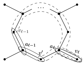
Figure 3. Direct step and cycle step

Definition 5.3.

For each path $\gamma_{L}\in\Gamma_{L}$, we say that $\gamma_{L}$ is a (relaxed) projected path if for each $1\leq\ell\in L$ it satisfies the five events $\mathsf{A}_{\ell},\mathsf{B}_{\ell},\mathsf{C}_{\ell},\mathsf{D}_{\ell}^{1},\mathsf{D}_{\ell}^{2}$ defined in (11) and for each $\ell\in I_{\textup{c}}$, it further satisfies

$$\textup{{G}}_{\ell}\equiv\left\{\begin{minipage}{260.17464pt} $\exists$ an alternating sequence $(\tilde{a}_{0}\tilde{v}_{0}\tilde{a}_{1}\tilde{v}_{1}\cdots\tilde{a}_{m}\tilde{v}_{m})$ such that: \begin{enumerate}[1.] \par\enumerate@item@$(\tilde{v}_{0},\tilde{a}_{0})=(v_{\ell-1},a_{\ell-1})$, $(\tilde{v}_{m},\tilde{a}_{m})=(v_{\ell},a_{\ell})$ \par\enumerate@item@$(\tilde{a}_{0}\tilde{v}_{0}\tilde{a}_{1}\tilde{v}_{1}\cdots\tilde{a}_{m}v^{\prime}_{\ell})$ completes a cycle in $G$. \par\enumerate@item@$\exists t_{\ell-1}=\tilde{t}_{0}\leq\tilde{t}_{1}<\cdots<\tilde{t}_{m-1}\leq\tilde{t}_{m}=t_{\ell}$, such that $(\tilde{v}_{r},\tilde{t}_{r})\in\xi^{\circ}$ for $1\leq r\leq m-2$. \par\end{enumerate} \end{minipage}\right\},$$

where $v^{\prime}_{\ell}$ is the vertex in $\partial a_{\ell}\cap\partial a_{\ell-1}$. Let $\tilde{\Gamma}_{\textup{proj},L}$ denotes the set of (relaxed) projected path.

Remark 5.4.

Recall the definition in Remark 4.6. The discussion preceding the definition implies that $\Gamma_{\textup{proj},L}\subseteq\tilde{\Gamma}_{\textup{proj},L}$. Meanwhile a path in $\tilde{\Gamma}_{\textup{proj},L}$ does not necessarily satisfy events $\{\mathsf{D}^{3}_{\ell}\}$. We also do not assume in the definition of $\textup{{G}}_{\ell}$ that the values of updates at $\{(\tilde{v}_{r},\tilde{t}_{r})\}$ are all ones (which turns out to be crucial in the proof). Hence the name relaxed.

Remark 5.5.

In the third requirement of the definition of $\textup{{G}}_{\ell}$, we require $(\tilde{v}_{r},\tilde{t}_{r})\in\xi^{\circ}$ for $1\leq r\leq m-2$ so that none of the $\tilde{v}_{r}$’s belong to $\partial a_{\ell-1}\cup\partial a_{\ell}$ and hence $\textup{{G}}_{\ell}$ and $\mathsf{B}_{\ell}$ depend on different vertices. In the proof, we shall condition on events of the form $\textup{{G}}_{\ell}$. While conditioning on updates with value one works against us, conditioning on having at earlier times updates with unspecified values can only work to our advantage.

We now outline the two-step recursion on $\tilde{\Gamma}_{\textup{proj},L}$ and the proof of Theorem 1.3. Most of the arguments are parallel to the corresponding parts in Section 4. With some abuse of notation, we occasionally override the notations in Section 4 with slightly different meanings.

Fix $\gamma_{L}=((v_{\ell},a_{\ell},t_{\ell}))_{0\leq\ell\leq L}\in\Gamma_{L}$ and vertex-hyperedge pair $(v,a)$ satisfying $a\in\mathbb{N}(a_{L}),v\in\partial a$, we let $\gamma_{L+1}(t)\equiv\gamma_{L+1}(v,a,t)$ be the path extended from $\gamma_{L}$ with $(v_{L+1},a_{L+1},t_{L+1})=(v,a,t)$ and define

$$N^{\textup{proj}}(v,a) \equiv N^{\textup{proj}}(v,a;\gamma_{L})\equiv|\{t:\gamma_{L+1}(v,a,t)\in\tilde{\Gamma}_{\textup{proj},L+1}\}|.$$

Lemma 5.6.

For any two neighbouring hyperedges $a\in F,b\in\mathbb{N}(a)$, let $R(a,b)$ be the length of the shortest cycle in $G$ that contains $a$ and $b$. There exists a constant $C_{1}>0$ such that for any integer $L\geq 1$, $\gamma_{L}\in\tilde{\Gamma}_{\textup{proj},L}$ and $a\in\mathbb{N}(a_{L})$, $v\in\partial a$,

$$\mathbb{E}[N^{\textup{proj}}(v,a)\mid\gamma_{L}\in\tilde{\Gamma}_{\textup{proj},L}]\leq{C_{1}}\begin{cases}1/k&a=a_{L},\\ 2^{-k}&a\neq a_{L},\partial a\cap\mathsf{cyc}^{+}(a_{L},v_{L})\neq\varnothing,\\ p_{\textup{c}}(R(a,a_{L}))&a\neq a_{L},\partial a\cap\mathsf{cyc}^{+}(a_{L},v_{L})=\varnothing,\end{cases}$$ (30)

where

$$p_{\textup{c}}(r)\equiv e^{-k}+k\sum_{m\geq r}(\Delta k)^{m}\mathbb{P}(\textup{Pois}(k)\geq m-2).$$

Proposition 5.7.

Denote $R_{\star}=R_{\star}(\Delta,k)\equiv\lceil e\Delta k^{2}\rceil+1$. Then that for all $\Delta\leq 2^{k}$, $\gamma_{L}\in\Gamma_{L}$, $r\geq 2R_{\star}$ and $1\leq\ell\leq L$,

$$p_{c}(r)\leq(1+2^{-e\Delta k^{2}})\cdot e^{-k}\leq 2e^{-k}.$$

Proof.

Let $R$ follows the Poisson$(k)$ distribution of parameter $k$. Using Stirling’s approximation, we have that $\mathbb{P}(R=m)\leq\frac{e^{-k}k^{m}}{m!}\leq\frac{e^{-k}}{\sqrt{2\pi m}}\left(\frac{ek}{m}\right)^{m}$. Hence $\mathbb{P}(R\geq m)\leq 2\mathbb{P}(R=m)$ for all $m\geq 2ek$. It follows that for all $r\geq\lceil 2e\Delta k^{2}\rceil+2$,

$$p_{c}(r)-e^{-k} =k\sum_{m\geq r}(\Delta k)^{m}\mathbb{P}(R\geq m-2)\leq 2\Delta k^{2}\sum_{m\geq r}\frac{e^{-k}}{\sqrt{2\pi(m-2)}}\left(\frac{e\Delta k^{2}}{m}\right)^{m-2}$$

$$\leq\frac{1}{2}\Delta ke^{-k}\sum_{i\geq r-2}2^{-i}\leq\Delta ke^{-k}2^{-(r-2)}\leq e^{-k}2^{-e\Delta k^{2}}.$$

This concludes the proof. ∎

Meanwhile, similarly to the definition of type-II branchings in redacted paths, special treatment is needed for paths staying at the same hyperedges three steps in a row. Fix $\gamma_{L}=((v_{\ell},a_{\ell},t_{\ell}))_{0\leq\ell\leq L}\in\Gamma_{L}$ and let vertices $v,v^{\prime}$ satisfy $v,v^{\prime}\in a_{L}$. Let $\gamma_{L+2}\equiv\gamma_{L+2}(v,v^{\prime},t,t^{\prime})=((v_{\ell},a_{\ell},t_{\ell}))_{0\leq\ell\leq L+2}\in\Gamma_{L+2}$ be the path extended from $\gamma_{L}$ with

$$(v_{L+2},a_{L+2},t_{L+2})=(v,a_{L},t),\quad(v_{L+1},a_{L+1},t_{L+1})=(v^{\prime},a_{L},t^{\prime}),$$

Observe that by construction, in order for $\gamma_{L+2}$ (as above) to be in $\tilde{\Gamma}_{\textup{proj},L+2}$, it must be the case that $a_{L}$ is deactivated w.r.t. itself by time $t$ (i.e., $t>T_{+}(a_{L};t_{L})$), making the event $Y_{t}(\partial a_{L})=\underline{1}$ unlikely (cf. the first case of Lemma 5.6). This is quantified in the following lemma. We define

$$N^{\textup{proj}}_{=}(v,v^{\prime})\equiv N^{\textup{proj}}_{=}(v,v^{\prime};\gamma_{L})\equiv|\{(t,t^{\prime}):\gamma_{L+2}(v,v^{\prime},t,t^{\prime})\in\tilde{\Gamma}_{\textup{proj},L+2}\}|.$$

Lemma 5.8.

Under the notations above, there exists an absolute constant $C_{2}>0$ such that

$$\mathbb{E}[N^{\textup{proj}}_{=}(v,v^{\prime};\gamma_{L})\mid\gamma_{L}\in\tilde{\Gamma}_{\textup{proj},L}]\leq{C_{2}}k^{2}2^{-k}.$$ (31)

For $r=1,2$, Let $N_{\textup{proj},L+r}(\gamma_{L})$ be the number of paths $\gamma_{L+r}\in\tilde{\Gamma}_{\textup{proj},L+r}$ that agree with $\gamma_{L}$ in the first $L$ steps and write $N^{\neq}_{\textup{proj},L+1}(\gamma_{L})$ (resp. $N^{=}_{\textup{proj},L+1}(\gamma_{L})$) for the number of paths $\gamma_{L+1}$’s counted in $N_{\textup{proj},L+1}(\gamma_{L})$ that further satisfies $a_{L+1}\neq a_{L}$ (resp. $a_{L+1}=a_{L}$). Lemma 5.6, Lemma 5.8 and Proposition 5.7 together imply the following theorem. The proof is presented for the sake of completeness.

Theorem 5.9.

Under the above notation, there exists an absolute constant $C_{\textup{proj}}>0$, such that for any $R_{\star}$-good hypergraph $G$, integer $L\geq 1$ and path $\gamma_{L}\in\Gamma_{L}$, we have that

$$\mathbb{E}[N^{=}_{\textup{proj},L+1}(\gamma_{L})\mid\gamma_{L}\in\tilde{\Gamma}_{\textup{proj},L}] \leq C_{\textup{proj}},$$ (32)

$$\mathbb{E}[N^{\neq}_{\textup{proj},L+1}(\gamma_{L})\mid\gamma_{L}\in\tilde{\Gamma}_{\textup{proj},L}] \leq C_{\textup{proj}}(\Delta k)2^{-k},$$ (33)

$$\mathbb{E}[N_{\textup{proj},L+2}(\gamma_{L})\mid\gamma_{L}\in\tilde{\Gamma}_{\textup{proj},L}] \leq C_{\textup{proj}}^{2}[(\Delta k2^{-k})+k^{4}2^{-k}].$$ (34)

Proof.

Fix $\gamma_{L}\equiv((v_{\ell},a_{\ell},t_{\ell}))_{1\leq\ell\leq L}\in\Gamma_{L}$ and for brevity define $\tilde{\mathbb{E}}_{L}\equiv\mathbb{E}[\,\cdot\mid\gamma_{L}\in\tilde{\Gamma}_{\textup{proj},L}]$. We first prove (32). By the first case of Lemma 5.6,

$$\tilde{\mathbb{E}}_{L}[N^{=}_{\textup{proj},L+1}(\gamma_{L})]=\sum_{v\in\partial a_{L}}\tilde{\mathbb{E}}_{L}[N^{\textup{proj}}(v,a_{L};\gamma_{L})]\leq k\cdot C_{1}k^{-1}.$$

We now prove (33), we define

$$A_{L+1}\equiv\{a\in\mathbb{N}(a_{L})\setminus{\{a_{L}\}}:\partial a\cap\mathsf{cyc}^{+}(a_{L},v_{L})=\varnothing\}$$

be the set of hyperedges that could form a direct branching from $(v_{L},a_{L},t_{L})$. It follows that

$$N^{\neq}_{\textup{proj},L+1}(\gamma_{L}) =\sum_{a\in A_{L+1}}\sum_{v\in\partial a}N^{\textup{proj}}(v,a;\gamma_{L})+\sum_{a\in\mathbb{N}(a_{L})\setminus(A_{L+1}\cup\{a_{L}\})}\sum_{v\in\partial a}N^{\textup{proj}}(v,a;\gamma_{L}).$$

Observe that every $a\in\mathbb{N}(a_{L})\setminus(A_{L+1}\cup\{a_{L}\})$ must satisfy $R(a,a_{L})\geq R_{\star}$. Applying the last two cases of Lemma 5.6 then yields

$$\tilde{\mathbb{E}}_{L}[N^{\neq}_{\textup{proj},L+1}(\gamma_{L})] \leq k|A_{L+1}|\cdot C_{1}2^{-k}+k|\mathbb{N}(a_{L})|\cdot C_{1}p_{c}(R_{\star})$$

$$\leq C_{1}[3k\Delta 2^{-k}+k\Delta\cdot kp_{c}(R^{\star})]\leq C_{\textup{proj}}\,\Delta k2^{-k}.$$

Finally, to prove (34), we note that the bound of Lemma 5.6 does not depend on $t_{L}$. Again we abbreviate $\tilde{\mathbb{E}}_{L+1}(\cdot)\equiv\mathbb{E}[\cdot\mid\gamma_{L+1}\in\tilde{\Gamma}_{\textup{proj},L+1}]$ and let $A_{L+1}$ be defined as in the previous case (with respect to the $(L+1)$’th step). There are three possible ways of extending $\gamma_{L}$ to $\gamma_{L+2}$:

$$a_{L}=a_{L+1}=a_{L+2}\textup{\quad or \quad}a_{L}=a_{L+1}\neq a_{L+2}\textup{\quad or \quad}a_{L}\neq a_{L+1}.$$

Following a similar argument as that of Theorem 4.14, we have that

$$\tilde{\mathbb{E}}[N_{\textup{proj},L+2}(\gamma_{L})] \leq\sum_{v,v^{\prime}\in a_{L}}\tilde{\mathbb{E}}_{L}[N^{\textup{proj}}_{=}(v,v^{\prime})]$$

$$+\sum_{a\neq a_{L}}\sum_{v\in\partial a}\tilde{\mathbb{E}}_{L}[N^{\textup{proj}}(v,a;\gamma_{L})]\cdot\tilde{\mathbb{E}}_{L+1}[N^{=}_{\textup{proj},L+2}(\gamma_{L+1}(v,a))]$$

$$+\sum_{v\in\partial a_{L}}\tilde{\mathbb{E}}_{L}[N^{\textup{proj}}(v,a_{L};\gamma_{L})]\cdot\tilde{\mathbb{E}}_{L+1}[N^{\neq}_{\textup{proj},L+2}(\gamma_{L+1}(v,a_{L}))].$$

Applying (32), (33) and Lemma 5.8 implies that

$$\tilde{\mathbb{E}}[N_{\textup{proj},L+2}(\gamma_{L})] \leq C_{2}k^{4}2^{-k}+\tilde{\mathbb{E}}_{L}[N^{\neq}_{\textup{proj},L+1}(\gamma_{L})]\max_{v,a:a\neq a_{L},v\in\partial a}\tilde{\mathbb{E}}_{L+1}[N^{=}_{\textup{proj},L+2}(\gamma_{L+1}(v,a))]$$

$$+\tilde{\mathbb{E}}_{L}[N^{=}_{\textup{proj},L+1}(\gamma_{L})]\max_{v\in\partial a_{L}}\tilde{\mathbb{E}}_{L+1}[N^{\neq}_{\textup{proj},L+2}(\gamma_{L+1}(v,a_{L}))]$$

$$\leq\textup{ RHS of \eqref{e:Nprojtwo},}$$

which concludes the proof. ∎

Proof of Theorem 1.3.

The assertion of Theorem 1.3 is obtained by combining Lemma 4.5, (15), Remark 5.4 and (34). ∎

5.2. Proof of Lemma 5.6 and Lemma 5.8

In this subsection we present the proofs of remaining lemmas. We begin with Lemma 5.6. Throughout the proof, we keep $\gamma_{L}\in\Gamma_{L},a\in\mathbb{N}(a_{L}),v\in\partial a$ fixed, and for brevity of notation write $\gamma_{L+1}(t)$ for the path extended from $\gamma_{L}$ with $(v_{L+1},a_{L+1},t_{L+1})=(v,a,t)$. We further define

$$\mathsf{M}^{\textup{c}}_{\ell}(t)\equiv\mathsf{M}^{\textup{c}}_{\ell}(\tilde{\gamma}_{L+1}(t)) \equiv\mathsf{A}_{\ell}(t)\cap\mathsf{B}_{\ell}(t)\cap\mathsf{C}_{\ell}(t)\cap\mathsf{D}^{1}_{\ell}(t)\cap\mathsf{D}^{2}_{\ell}(t)\cap\textup{{G}}_{\ell}(t) \forall\ell\in I_{\textup{c}}(\gamma_{L+1}(t)),$$

$$\mathsf{M}^{\textup{d}}_{\ell}(t)\equiv\mathsf{M}^{\textup{d}}_{\ell}(\tilde{\gamma}_{L+1}(t)) \equiv\mathsf{A}_{\ell}(t)\cap\mathsf{B}_{\ell}(t)\cap\mathsf{C}_{\ell}(t)\cap\mathsf{D}^{1}_{\ell}(t)\cap\mathsf{D}^{2}_{\ell}(t) \forall\ell\in I_{\textup{d}}(\gamma_{L+1}(t)),$$

where we henceforth omit $t$ from the notation for all events with $\ell\leq L$, as they do not depend on the value of $t$. We further write (overriding any conflicting definitions from Section 4)

$$\mathsf{N}_{L}\equiv\{\gamma_{L}\in\tilde{\Gamma}_{\textup{proj},L}\}=\Big{[}\cap_{\ell\in I_{\textup{c}}}\mathsf{M}^{\textup{c}}_{\ell}\Big{]}\bigcap\Big{[}\cap_{\ell\in I_{\textup{d}}}\mathsf{M}^{\textup{d}}_{\ell}\Big{]}.$$

By Campbell’s theorem,

$$\mathbb{E}[N^{\textup{proj}}(v,a)\,|\,\gamma_{L}\in\tilde{\Gamma}_{\textup{proj},L}] =\mathbb{E}\Big{[}\!\sum_{t:(v,t,1)\in\xi}\!\!\mathbf{1}\{\mathsf{M}^{\bullet}_{L+1}(t)\}\,\Big{|}\,\mathsf{N}_{L}\Big{]}=\frac{1}{2}\int_{t_{L}}^{\infty}\mathbb{P}(\mathsf{M}^{\bullet}_{L+1}(t)\,|\,\mathsf{N}_{L},\mathsf{A}_{L+1}(t))dt.$$

where $\bullet=\textup{c}$ if $L+1\in I_{\textup{c}}$ and $\bullet=\textup{d}$ otherwise.

Lemma 5.10.

Under the notations above,

$$\mathbb{P}(\mathsf{M}^{\textup{d}}_{L+1}(t)\mid\mathsf{N}_{L},\mathsf{A}_{L+1}(t))\leq\begin{cases}2^{2-k}\mathbb{P}(\mathsf{B}_{L+1}(t))&a\neq a_{L}\\ \mathbb{P}(\mathsf{B}_{L+1}(t))&a=a_{L}\end{cases}.$$

Moreover if $L+1\in I_{\textup{c}}(\gamma_{L+1}(t))$, then

$$\mathbb{P}(\mathsf{M}^{\textup{c}}_{L+1}(t)\mid\mathsf{N}_{L},\mathsf{A}_{L+1}(t))\leq 2^{1-k}\mathbb{P}(\textup{{G}}_{L+1}(t))\mathbb{P}(\mathsf{B}_{L+1}(t)).$$

Proof.

Recall the definition of $\ell_{-}(u),\mathcal{F}_{L+1},\mathsf{N}^{\circ}_{L},\mathsf{C}^{\prime}_{L+1}$ from the proof of Lemma 4.15 and omit $t$ from the notation. By the Markov property of the process $Y_{t}$, the events $\mathsf{A}_{L+1}$, $\mathsf{B}_{L+1}$, $\mathsf{C}^{\prime}_{L+1}$, $\mathsf{D}^{1}_{L+1}$, $\mathsf{D}^{2}_{L+1}$ and (in the case of $L+1\in I_{\textup{c}}$) $\textup{{G}}_{L+1}$ are independent of $\mathcal{F}_{L+1}$ given $\mathsf{N}^{\circ}_{L}$. Meanwhile, for each $1\leq\ell\leq L$, we have that $\mathsf{M}^{\textup{d}}_{\ell}$ is measurable w.r.t. $\mathcal{F}_{L+1}$. It is left to treat $\{\textup{{G}}_{\ell}\}_{\ell\in I_{\textup{c}}}$.

Observe that for each $\ell\in I_{\textup{c}}$, we have that $\textup{{G}}_{\ell}$ is a measurable function of $\xi^{\circ}(V\times{[}t_{\ell-1},t_{\ell}))$, the time and locations of all updates between $t_{\ell-1}$ and $t_{\ell}$ without the value of the updates. Following a similar argument of Lemma 4.15, we define

$$W_{\ell}\equiv\{u\in\partial a_{\ell-1}\cap\partial a_{\ell}^{c}:u\in(\partial a\cap\partial a_{L}^{c})\setminus\{v\},\ell_{-}(u)=\ell-1\}$$

and (overriding the definition in Lemma 4.15)

$$\tilde{W}_{\ell}\equiv W_{\ell}\times{[}t_{\ell-1},t_{\ell}),\quad\tilde{V}_{\ell}\equiv W_{\ell}^{c}\times{[}t_{\ell-1},t_{\ell}).$$

Let $\Xi_{\ell}(\tilde{W}_{\ell})$ be the range of the unmarked update process $\xi^{\circ}(\tilde{W}_{\ell})$ over $\textup{{G}}_{\ell}$ (i.e., the collection of all possible values of $\xi^{\circ}(\tilde{W}_{\ell})$, provided that $\textup{{G}}_{\ell}$ occurs). It follows that

$$\textup{{G}}_{\ell}=\cup_{\xi^{\circ}(\tilde{W}_{\ell})\in\Xi_{\ell}(\tilde{W}_{\ell})}\{\xi^{\circ}(\tilde{W}_{\ell})\}\times\{\xi^{\circ}(\tilde{V}_{\ell}):\xi^{\circ}(\tilde{W}_{\ell}\cup\tilde{V}_{\ell})\in\textup{{G}}_{\ell}\},$$

where $\xi^{\circ}(\tilde{W}_{\ell})$ is independent of $\mathcal{F}_{L+1}$ and $\xi^{\circ}(\tilde{V}_{\ell})$ is $\mathcal{F}_{L+1}$-measurable. Therefore following a similar calculation to (28), we have

$$\mathbb{P}(\mathsf{M}^{\textup{d}}_{L+1}(t)\mid\mathsf{N}_{L},A_{L+1}(t))$$

$$\leq\sup_{\xi^{\circ}(\tilde{W}_{\ell})\in\Xi_{\ell}(\tilde{W}_{\ell})}\mathbb{P}(\mathsf{D}^{1}_{L+1}\mid\mathsf{N}^{\circ}_{L},\mathsf{C}^{\prime}_{L+1},\{\xi^{\circ}(\tilde{W}_{\ell})\}_{\ell\in I_{\textup{c}}})\cdot\mathbb{P}(\mathsf{B}_{L+1},\mathsf{D}^{2}_{L+1}\mid\mathsf{N}^{\circ}_{L})$$

$$\leq 2^{-(k-2)\mathbf{1}\{a\neq a_{L}\}}\mathbb{P}(\mathsf{B}_{L+1}),$$ (35)

where for the last step, we note that for $G\in\mathcal{G}$, we have that $|\partial a\cap\partial a_{L}|\leq 2$ if $a\neq a_{L}$.

Recall that the definition of $\textup{{G}}_{L+1}$ does not involve the updates on $\partial a_{L}\cup\partial a$. The result for $\mathsf{M}^{\textup{c}}_{L+1}$ follows a similar argument to that of (35). ∎

Proof of Lemma 5.6.

The first two cases follow from a similar argument to that of Lemma 4.12 with overlap $m_{L+1}=k$ and $m_{L+1}\leq 2$, respectively. Here we only present the proof of the third case, leaving the first two as an exercise. Fix $(v,a)$ such that $a\neq a_{L}$ and $\partial a\cap\mathsf{cyc}^{+}(a_{L},v_{L})=\varnothing$. Let $\gamma_{L+1}=\gamma_{L+1}(v,a;\gamma_{L})$. We can write

$$\int_{t_{L}}^{\infty}\mathbb{P}(\textup{{G}}_{L+1}(t))\mathbb{P}(\mathsf{B}_{L+1}(t))dt \leq\int_{t_{L}}^{t_{L}+k}\mathbb{P}(\textup{{G}}_{L+1}(t))dt+\int_{t_{L}+k}^{\infty}\mathbb{P}(\mathsf{B}_{L+1}(t))dt.$$

$$\leq k\mathbb{P}(\textup{{G}}_{L+1}(t_{L}+k))+\mathbb{P}(T_{+}(a_{L+1};a_{L},t_{L})>t_{L}+k)$$ (36)

Since in a cycle step $|\partial a_{L}\cap\partial a_{L+1}|=1$, the second term on the RHS of (36) can be bounded by $e^{-k}$. For the first term, we enumerate over all possible cycles containing $a_{L},a_{L+1}$. Fix some cycle $(\tilde{a}_{0}\tilde{v}_{0}\tilde{a}_{1}\dots\tilde{a}_{m}\tilde{v}_{m})$ with $\tilde{a}_{0}=a_{L}$ and $\tilde{a}_{m}=a_{L+1}$. Let $s_{0}\equiv t_{L}$ and inductively define $s_{i}=T(\tilde{v}_{i};s_{i-1})$, for all $1\leq i\leq m-2$. Denote $\delta_{i}\equiv s_{i}-s_{i-1}$ and $S\equiv\sum_{i=1}^{m-2}\delta_{i}$. Then $\delta_{1},\ldots,\delta_{m-2}$ are i.i.d. Exp($1$) r.v.’s. In particular, interpreting the $\delta_{i}$’s as spacings between arrivals of a rate 1 Poisson process, we get that $\mathbb{P}(S\leq k)=\mathbb{P}(N_{k}\geq m-2)$, where $N_{k}$ has a Poisson distribution of parameter $k$. In conclusion,

$$\mathbb{P}(\tilde{v}_{1},\dots,\tilde{v}_{m-2}\textup{ are sequentially updated during }(t_{L},t_{L}+k))=\mathbb{P}(S\leq k)=\mathbb{P}(N_{k}\geq m-2).$$

Noting that there are at most $(\Delta k)^{m}$ cycles of length $m$ containing $a_{L}$ finishes the proof. ∎

We now prove Lemma 5.8. Fix $\gamma_{L}\in\Gamma_{L}$ and $v,v^{\prime}\in a_{L}$. We define the events $\mathsf{M}^{\textup{d}}_{\ell}$, $\mathsf{M}^{\textup{d}}_{L+1}(t^{\prime})$ and $\mathsf{M}^{\textup{d}}_{L+2}(t)$ in a similar fashion as $\mathsf{M}^{\textup{d}}_{\ell}$, $\mathsf{M}^{\textup{d}}_{L+1}(t)$ in the proof of Lemma 5.6. Observe that any $\gamma_{L+2}\equiv\gamma_{L+2}(v,v^{\prime},t,t^{\prime})$, must satisfy that $L+1,L+2\in I_{\textup{d}}$. By Campbell’s theorem,

$$\mathbb{E}[N^{\textup{proj}}_{2}\mid\gamma_{L}\in\tilde{\Gamma}_{\textup{proj},L}] =\mathbb{E}\Big{[}\sum_{\begin{subarray}{c}t>t^{\prime}:(v,t,1),(v^{\prime},t^{\prime},1)\in\xi\end{subarray}}\mathbf{1}\{\mathsf{M}^{\textup{d}}_{L+1}(t^{\prime})\}\cdot\mathbf{1}\{\mathsf{M}^{\textup{d}}_{L+2}(t)\}\ \Big{|}\ \mathsf{N}_{L}\Big{]}$$

$$=\frac{1}{4}\int_{t_{L}}^{\infty}\int_{t_{L}}^{t}\mathbb{P}(\mathsf{M}^{\textup{d}}_{L+2}(t),\mathsf{M}^{\textup{d}}_{L+1}(t^{\prime})\mid\mathsf{N}_{L},\mathsf{A}_{L+1}(t^{\prime}),\mathsf{A}_{L+2}(t))dtdt^{\prime}.$$

Proof of Lemma 5.8.

Following a similar argument of Lemma 5.10 we can show that for each $\gamma_{L+2}(v,v^{\prime},t,t^{\prime})\in\Gamma_{L+2}$,

$$\mathbb{P}(\mathsf{M}^{\textup{d}}_{L+2}(t),\mathsf{M}^{\textup{d}}_{L+1}(t^{\prime})\mid\mathsf{N}_{L},\mathsf{A}_{L+1}(t^{\prime}),\mathsf{A}_{L+2}(t))$$

$$\leq\mathbb{P}(\mathsf{B}_{L+1}(t^{\prime}),\mathsf{B}_{L+2}(t))\cdot\mathbb{P}(\mathsf{D}^{2}_{L+2}(t)\mid\mathsf{N}^{\circ}_{L},\mathsf{C}^{\prime}_{L+2}(t),\mathsf{B}_{L+1}(t^{\prime}),\mathsf{B}_{L+2}(t)))$$

$$\leq 2^{1-k}\mathbb{P}(\mathsf{B}_{L+1}(t^{\prime}),\mathsf{B}_{L+2}(t)),$$ (37)

where in the second step we ignored the event $\mathsf{D}^{2}_{L+1}(t^{\prime})$ and in the last step we used the independency between $Y_{t}(a_{L})$ and $Y_{t_{L}}(a_{L})$ given $\mathsf{C}^{\prime}_{L+2}(t)$.

Now let $T_{1}\equiv T_{+}(a_{L};a_{L},t_{L})$ and $T_{2}\equiv T_{+}(a_{L};a_{L},T_{1})$. By monotonicity of deactivation time, event $\mathsf{B}_{L+2}(t)\subseteq\{T_{2}>t\}$. Integrating the RHS of (37) over $t,t^{\prime}$, we have

$$\mathbb{E}[N^{\textup{proj}}_{2}\mid\gamma_{L}\in\tilde{\Gamma}_{\textup{proj},L}]\leq 2^{-(k+1)}\int_{t_{L}}^{\infty}(t-t_{L})\mathbb{P}(T_{2}>t)dt=2^{-(k+1)}\mathbb{E}(T_{2}-t_{L})^{2}.$$

Both $(T_{1}-t_{L})$ and $(T_{2}-T_{1})$ are distributed as the maximum of $k$ i.i.d. Exp(1) random variables and they are independent with each other. Therefore a very crude bound gives

$$\mathbb{E}(T_{2}-t_{L})^{2}\leq 4\mathbb{E}(T_{1}-t_{L})^{2}\leq 4k^{2}\mathbb{E}_{X\sim\textup{Exp}(1)}[X^{2}]\leq 8k^{2}.$$

Plugging the last inequality into (37) concludes the proof. ∎

6. From sampling to counting

In this section we derive Corollary 1.2 from our main result. The corollary follows from the rapid mixing of the Markov chain and following lemma, which is an analog of [7, Appendix A] and [1, Lemma 5]. Let $\mathcal{G}(k,\Delta)$ be the set of $k$-uniform hypergraphs of maximal degree $\Delta$.

Lemma 6.1.

Let $k$ and $\Delta$ be positive integers and $\mathcal{G}\subseteq\mathcal{G}(k,\Delta)$ be a subset of $\mathcal{G}(k,\Delta)$ that is closed under removal of hyperedges. Suppose that for each $\Delta,k$, there is a polynomial-time algorithm (in $n$ and $1/\epsilon$) that takes a hypergraph $G=(V,F,E)\in\mathcal{G}$ with at most $n$ vertices, a vertex $v\in V$ and an $\epsilon>0$ and outputs a quantity $p(v;G)$ satisfying

$$\left|\frac{p(v;G)}{\mathbb{P}_{G}(\sigma_{v}=0)}-1\right|<\epsilon.$$

with probability $1-\epsilon/n$, where $\sigma$ is a uniformly sampled independent set on $G$. Then there exists an FPRAS which approximates $Z(G)$ for all hypergraphs in $\mathcal{G}$.

Proof.

The proof is a slight modification from the argument in [1, Lemma 5] which we only include here for the sake of completeness. Fix $\epsilon>0$ and $G=(V,F,E)\in\mathcal{G}\subseteq\mathcal{G}(k,\Delta)$. Without loss of generality, we suppose $V\equiv[n]\equiv\{1,\dots,n\}$. Let $G_{0}\equiv G$ and for each $1\leq i\leq n-1$, let $G_{i}$ be the remaining hypergraph after removing the first $i$ vertices $[i]\equiv\{1,\dots,i\}$ along with all hyperedges containing at least one vertex in $[i]$. The set of independent sets on $G_{i}$ can be naturally identified with the subset of independent sets on $G$ satisfying $\sigma|_{\{1,\dots,i\}}=\underline{0}$. We have

$$\frac{1}{Z(G)} =\mathbb{P}_{G}(\underline{\sigma}=\underline{0})=\mathbb{P}(\sigma_{1}=0)\prod_{i=2}^{n}\mathbb{P}_{G}(\sigma_{i}=0\mid\sigma_{[i-1]}=0)=\prod_{i=1}^{n}\mathbb{P}_{G_{i-1}}(\sigma_{i}=0).$$

By assumption, the set $\mathcal{G}$ is closed under the removal of hyperedges, thus if $G\in\mathcal{G}$, then so is every $G_{i}$, for all $1\leq i\leq n-1$. Consequently, we can compute (in $\textup{poly}(n,1/\epsilon)$ time) quantities $p_{i}\equiv p(i;G_{i-1})$ such that

$$\left|\frac{p(i;G_{i-1})}{\mathbb{P}_{G_{i-1}}(\sigma_{i}=0)}-1\right|<\frac{\epsilon}{2n},$$

with probability $1-\epsilon/n$. Letting $\hat{Z}(G)\equiv\prod_{i=1}^{n}p(i;G_{i-1})$ be the output concludes the proof. ∎

Proof of Corollary 1.2.

Following the statement of Lemma 6.1, we set $\mathcal{G}=\mathcal{G}(k,\Delta)$ and describe the $p(v,G)$-outputting algorithm as follows: Given hypergraph $G$ and $n,\epsilon>0$, let $t_{\textup{mix}}=O(n\log n)$ be the mixing time of the Glauber dynamics of hypergraph independent set on $G$ and let $N,M$ be two large integers to be determined shortly. We run the Glauber dynamics $N$ times for $M\cdot t_{\textup{mix}}$ steps, starting from the all zeros configuration, and record the configuration at time $M\cdot t_{\textup{mix}}$ of the $r$’th sample by $\sigma^{(r)}$. We set $M\equiv 1+2\lceil|\log\epsilon|/\log 2\rceil$. By the submultiplicity property $t_{\textup{mix}}(2^{-i})\leq it_{\textup{mix}}$ [6, page 55] we have that

$$\big{|}\mathbb{P}(\sigma^{(1)}_{v}=0)-\mathbb{P}_{G}(\sigma_{v}=0)\big{|}\leq 2\|\mathbb{P}(\sigma^{(1)}=\cdot)-\mathbb{P}_{G}(\sigma=\cdot)\|_{\mathrm{TV}}\leq 2^{-(M-1)}\leq\epsilon^{2}<\epsilon/4,$$

where $\sigma$ is a uniformly chosen independent set. We set $N\equiv 32\lceil|\log\epsilon|\rceil/\epsilon^{2}$ and $p(v;G)\equiv\frac{1}{N}\sum_{r=1}^{N}\mathbf{1}\{\sigma^{(r)}_{v}=0\}.$ By Azuma-Hoeffding’s inequality,

$$\mathbb{P}\big{(}|p(v;G)-\mathbb{P}(\sigma^{(1)}_{v}=0)|>\epsilon/4\big{)}\leq e^{-N\epsilon^{2}/32}\leq\epsilon.$$

Note that $\mathbb{P}_{G}(\sigma_{v}=0)\geq 1/2$ for any hypergraph $G=(V,F)$ and all $v\in V$. Combining the last two displays then guarantees that $|p(v;G)/\mathbb{P}(\sigma_{v}=0)-1|<\epsilon$ with probability $1-\epsilon$. The total running time of our algorithm is $N\cdot M\cdot t_{\textup{mix}}$, which by Theorem 1.1 is $\textup{poly}(n,1/\epsilon)$. ∎

References

- [1] Ivona Bezáková, Andreas Galanis, Leslie Ann Goldberg, Heng Guo, and Daniel Štefankovič. Approximation via correlation decay when strong spatial mixing fails. In 43rd International Colloquium on Automata, Languages, and Programming, ICALP 2016, July 11-15, 2016, Rome, Italy, pages 45:1–45:13, 2016.
- [2] Magnus Bordewich, Martin Dyer, and Marek Karpinski. Stopping times, metrics and approximate counting. In International Colloquium on Automata, Languages, and Programming, pages 108–119. Springer, 2006.
- [3] Magnus Bordewich, Martin Dyer, and Marek Karpinski. Path coupling using stopping times and counting independent sets and colorings in hypergraphs. Random Structures & Algorithms, 32(3):375–399, 2008.
- [4] Heng Guo, Mark Jerrum, and Jingcheng Liu. Uniform sampling through the Lovász Local Lemma. arXiv preprint arXiv:1611.01647, 2016.
- [5] Mark Jerrum and Alistair Sinclair. Polynomial-time approximation algorithms for the Ising model. SIAM Journal on computing, 22(5):1087–1116, 1993.
- [6] David Asher Levin, Yuval Peres, and Elizabeth Lee Wilmer. Markov chains and mixing times. American Mathematical Soc., 2009.
- [7] Jingcheng Liu and Pinyan Lu. FPTAS for counting monotone CNF. In Proceedings of the Twenty-Sixth Annual ACM-SIAM Symposium on Discrete Algorithms, pages 1531–1548. SIAM, 2015.
- [8] Eyal Lubetzky and Allan Sly. Cutoff phenomena for random walks on random regular graphs. Duke Mathematical Journal, 153(3):475–510, 2010.
- [9] Eyal Lubetzky and Allan Sly. Information percolation and cutoff for the stochastic Ising model. Journal of the American Mathematical Society, 2015.
- [10] Ankur Moitra. Approximate counting, the Lovasz Local Lemma and inference in graphical models. arXiv preprint arXiv:1610.04317, 2016.
- [11] Robin A Moser. A constructive proof of the lovász local lemma. In Proceedings of the forty-first annual ACM symposium on Theory of computing, pages 343–350. ACM, 2009.
- [12] Alistair Sinclair, Piyush Srivastava, and Marc Thurley. Approximation algorithms for two-state anti-ferromagnetic spin systems on bounded degree graphs. Journal of Statistical Physics, 155(4):666–686, 2014.
- [13] Allan Sly. Computational transition at the uniqueness threshold. In Foundations of Computer Science (FOCS), 2010 51st Annual IEEE Symposium on, pages 287–296. IEEE, 2010.
- [14] Allan Sly and Nike Sun. The computational hardness of counting in two-spin models on d-regular graphs. In Foundations of Computer Science (FOCS), 2012 IEEE 53rd Annual Symposium on, pages 361–369. IEEE, 2012.
- [15] Dror Weitz. Counting independent sets up to the tree threshold. In Proceedings of the thirty-eighth annual ACM symposium on Theory of computing, pages 140–149. ACM, 2006.