Quantum electrodynamic approach to the conductivity of gapped graphene

Abstract

The electrical conductivity of graphene with a nonzero mass-gap parameter is investigated starting from the first principles of quantum electrodynamics in (2+1)-dimensional space-time at any temperature. The formalism of the polarization tensor defined over the entire plane of complex frequency is used. At zero temperature we reproduce the results for both real and imaginary parts of the conductivity, obtained previously in the local approximation, and generalize them taking into account the effects of nonlocality. At nonzero temperature the exact analytic expressions for real and imaginary parts of the longitudinal and transverse conductivities of gapped graphene are derived, as well as their local limits and approximate expressions in several asymptotic regimes. Specifically, a simple local result for the real part of conductivity of gapped graphene valid at any temperature is obtained. According to our results, the real part of the conductivity is not equal to zero for frequencies exceeding the width of the gap and goes to the universal conductivity with increasing frequency. The imaginary part of conductivity of gapped graphene varies from infinity at zero frequency to minus infinity at the frequency defined by the gap parameter and then goes to zero with further increase of frequency. The analytic expressions are accompanied by the results of numerical computations. Possible future generalization of the used formalism is discussed.

I Introduction

During the last few years, a two-dimensional hexagonal lattice of carbon atoms known as graphene has attracted widespread attention owing to its unusual physical properties and promising applications 1 . Unlike conventional condensed matter systems, the quasiparticles in graphene are massless or very light particles which at low energies obey the relativistic Dirac equation, where the speed of light $c$ is replaced with the Fermi velocity $v_{F}\approx c/300$ (see the monograph 1 and review papers 2 ; 3 ; 4 ). This makes the electronic properties of graphene highly nontrivial, and, specifically, results in the existence 5 of a universal (up to small nonlocal corrections) frequency-independent conductivity $\sigma_{0}$ in the limit of zero temperature.

The electrical conductivity of graphene was investigated in many theoretical papers using the current-current correlation functions in the random phase approximation, the two-dimensional Drude model, the quasiclassical approach, the Kubo formula, and Boltzmann’s transport theory (see, e.g., Refs. 6 ; 7 ; 8 ; 9 ; 10 ; 11 ; 12 ; 13 ; 14 ; 15 ; 16 ; 17 ; 18 ; 19 ; 20 ; 21 ; 22 ; 23 ; 24 ; 25 ; 26 ; 27 ; 28 ; 29 ; 30 ). At first, a few distinct values for the universal conductivity $\sigma_{0}$ have been obtained by different authors (see Refs. 4 ; 9 ; 10 ; 21 for a review) depending on the order of limiting transitions in the used theoretical approach. At a later time, a consensus was achieved on the value $\sigma_{0}=e^{2}/(4\hbar)$ 5 ; 6 ; 13 ; 18 ; 21 ; 27 ; 30 . However, up to now there is no complete agreement between the results of the different approximate and phenomenological approaches to the conductivity of graphene at nonzero temperature, in the presence of nonzero mass-gap parameter and chemical potential. In doing so, the experimental results 31 ; 32 ; 33 ; 34 ; 35 are not of sufficient precision for a clear discrimination between the various theoretical predictions.

Quantum electrodynamics at nonzero temperature provides a regular way for describing the response of a physical system to the electromagnetic field by means of polarization tensor. For graphene with an arbitrary mass-gap parameter $\Delta$ an explicit expression for the polarization tensor in (2+1)-dimensional space-time was found in Ref. 36 at zero temperature. The temperature correction to the polarization tensor of graphene was derived in Ref. 37 at the pure imaginary Matsubara frequencies. The results of Refs. 36 ; 37 have been used to calculate the Casimir and Casimir-Polder forces 37a ; 37b in many real physical systems incorporating graphene sheets 38 ; 39 ; 40 ; 41 ; 42 ; 43 ; 44 ; 45 (previously such calculations were performed by means of the density-density correlation functions of graphene, the spatially nonlocal dielectric permittivities, phenomenological Drude model, etc. 46 ; 47 ; 48 ; 49 ; 50 ; 51 ). The polarization tensor of graphene was also used 41 ; 52 to compare with theory the experimental data on measuring the Casimir interaction in graphene systems 53 , and very good agreement was obtained.

Another representation for the polarization tensor of graphene valid over the entire plane of complex frequency was derived in Ref. 54 . It was applied to investigate the origin of large thermal effect in the Casimir interaction between two graphene sheets 55 ; 55a and to calculate the reflectivity properties of gapless graphene 54 . In Ref. 57 the same polarization tensor allowed calculation of the reflectivity properties of graphene-coated substrates.

The derivation of the polarization tensor valid along the real frequency axis made it possible to investigate the electrical conductivity of graphene on the basis of first principles of quantum electrodynamics at nonzero temperature. Note that in Ref. 54 explicit expressions for the polarization tensor at real frequencies were obtained only for a pure (pristine) graphene having a zero mass-gap parameter, whereas for a gapped graphene the respective expressions were presented in an implicit form. Because of this, as the starting point, the conductivity of pure graphene was investigated 58 . In doing so, a few results obtained previously using different theoretical approaches have been reproduced, and several novel analytic asymptotic expressions and numerical results (especially for the imaginary part of conductivity) have been obtained.

In this paper we apply the formalism of the polarization tensor to systematically investigate the electrical conductivity of gapped graphene on the solid foundation of quantum electrodynamics. For this purpose, an explicit form of the results of Ref. 54 related to the case of nonzero mass-gap parameter is employed, which was found in Ref. 56 . It is known that quasiparticles in graphene may acquire some small mass $m$ under the influence of impurities, electron-electron interactions, and in the presence of substrates 2 ; 59 ; 60 ; 61 . The conductivity of gapped graphene was studied in Ref. 20 using the two-band model and in Ref. 29 using the static polarization function. At zero temperature some analytic expressions for the conductivity of gapped graphene were obtained in Refs. 16 ; 17 , whereas Ref. 27 contains the final results for both real and imaginary parts of conductivity in the local approximation. We reproduce the zero-temperature analytic results of Ref. 27 within the formalism of the polarization tensor and generalize them taking into account the effects of nonlocality. Specifically, it is shown that at zero temperature the real part of the conductivity of gapped graphene is equal to zero in the frequency region from zero to the characteristic frequency, which is slightly larger than $\Delta/\hbar$ due to nonlocal effects. With increasing frequency the real part of conductivity decreases monotonously from $2\sigma_{0}$ to $\sigma_{0}$.

According to our results, nonzero temperature has a dramatic impact on the conductivity of gapped graphene. Thus, the real part of conductivity for frequencies larger than the characteristic frequency may be either decreasing or increasing function depending on the relationship between the mass-gap parameter and the temperature. The imaginary part of the conductivity of gapped graphene varies from plus to minus infinity when frequency increases from zero to the characteristic frequency (at zero temperature it varies from zero to minus infinity in the same frequency region). We obtain the analytic asymptotic expressions and perform numerical computations for both real and imaginary parts of the conductivity of gapped graphene at nonzero temperature.

The paper is organized as follows. In Sec. II, we present explicit expressions for the polarization tensor of gapped graphene along the real frequency axis. In Sec. III, both real and imaginary parts of the conductivity of gapped graphene are derived at zero temperature. Sections IV and V investigate the impact of nonzero temperature on real and imaginary parts of the conductivity of gapped graphene, respectively. Our conclusions and discussion are contained in Sec. VI.

II Polarization tensor of gapped graphene

Here, we present analytic results for the polarization tensor of gapped graphene along the real frequency axis derived in Refs. 54 ; 56 . We also demonstrate how real and imaginary parts of the conductivity of graphene are expressed via imaginary and real parts of the polarization tensor, respectively. Both the longitudinal (along the graphene surface) and transverse (normal to the graphene surface) conductivities are considered.

The description of graphene using the polarization tensor in the one-loop approximation and the density-density correlation functions in the random phase approximation are equivalent 42 . The former method is, however, somewhat advantageous because it relies on well understood formalism of quantum field theory at nonzero temperature. This allowed complete derivation of the polarization tensor of gapped graphene valid over the entire plane of complex frequency 54 . In Ref. 56 a more convenient form of this tensor especially along the real frequency axis has been obtained for a gapped graphene.

As usual, we notate the polarization tensor as $\Pi_{\mu\nu}(\omega,k,T)$, where $\mu,\,\nu=0,\,1,\,2$, $\omega$ is the frequency of an electromagnetic wave, $k$ is the magnitude of the wave vector component parallel to graphene, and $T$ is the temperature. We assume real photons on a mass-shell, so that the inequality $k\leq\omega/c$ is satisfied. It has been shown 36 ; 37 that only the two components of the polarization tensor of graphene are independent. It is conventional to use $\Pi_{00}$ and $\Pi_{\rm tr}\equiv\Pi_{\mu}^{\,\mu}$ as the two independent quantities. For our purposes, however, it is more convenient to use the following combination

$$\Pi(\omega,k,T)\equiv k^{2}\Pi_{\rm tr}(\omega,k,T)+\left(\frac{\omega^{2}}{c^{2}}-k^{2}\right)\Pi_{00}(\omega,k,T)$$ (1)

as the second quantity.

We present $\Pi_{00}$ and $\Pi$ as the sums of zero-temperature contributions and temperature corrections

$$\Pi_{00}(\omega,k,T)=\Pi_{00}^{(0)}(\omega,k)+\Delta_{T}\Pi_{00}(\omega,k,T),$$

$$\Pi(\omega,k,T)=\Pi^{(0)}(\omega,k)+\Delta_{T}\Pi(\omega,k,T).$$ (2)

The thermal corrections $\Delta_{T}\Pi_{00}$ and $\Delta_{T}\Pi$ vanish in the limit of zero temperature.

The analytic expressions for the polarization tensor of gapped graphene at $T=0$ were derived in Ref. 36 . They result in

$$\Pi_{00}^{(0)}(\omega,k)=-\frac{\alpha k^{2}c^{2}}{\omega^{2}\eta^{2}}\Phi(\omega,k),$$

$$\Pi^{(0)}(\omega,k)=\alpha k^{2}\Phi(\omega,k),$$ (3)

where $\alpha=e^{2}/(\hbar c)$ is the fine structure constant, the quantity $\eta$ is defined as

$$\eta\equiv\eta(\omega,k)=\sqrt{1-\frac{v_{F}^{2}k^{2}}{\omega^{2}}}$$ (4)

and the function $\Phi$ along the real frequency axis is given by 54

$$\Phi(\omega,k)=\left\{\begin{array}[]{ll}\frac{2\Delta}{c}-\frac{2\hbar\omega\eta}{c}\left[1+\left(\frac{\Delta}{\hbar\omega\eta}\right)^{2}\right]{\rm arctanh}\frac{\hbar\omega\eta}{\Delta},&\hbar\omega<\frac{\Delta}{\eta},\\[8.53581pt] \frac{2\Delta}{c}-\frac{2\hbar\omega\eta}{c}\left[1+\left(\frac{\Delta}{\hbar\omega\eta}\right)^{2}\right]\left({\rm arctanh}\frac{\Delta}{\hbar\omega\eta}+i\frac{\pi}{2}\right),&\hbar\omega\geq\frac{\Delta}{\eta}.\end{array}\right.$$ (5)

Here, the energy gap $\Delta=2mc^{2}$ and $m$ is the mass of a quasiparticle (according to some estimations 36 $mc^{2}$ may achieve 0.1 eV).

As is seen from Eqs. (3)–(5), under the condition $\hbar\omega\eta<\Delta$ the quantities $\Pi_{00}^{(0)}$ and $\Pi^{(0)}$ are real. If the condition $\hbar\omega\eta\geq\Delta$ is satisfied, they have both real and imaginary parts.

We now continue by considering the thermal corrections in Eq. (2). The imaginary parts of both $\Delta_{T}\Pi_{00}$ and $\Delta_{T}\Pi$ are also different from zero only under the condition $\hbar\omega\eta\geq\Delta$ 54 ; 56 . The explicit forms are the following 54 ; 56 :

$${\rm Im}\Delta_{T}\Pi_{00}(\omega,k,T)=\frac{8\alpha\hbar c^{2}}{v_{F}^{2}}\int_{u^{(-)}}^{u^{(+)}}\!\!\!\frac{du}{e^{\beta u}+1}\frac{(2cu-\omega)^{2}-v_{F}^{2}k^{2}}{\omega\eta\sqrt{v_{F}^{2}k^{2}A(\omega,k)-(2cu-\omega)^{2}}},$$

(6)

$${\rm Im}\Delta_{T}\Pi(\omega,k,T)=\frac{8\alpha\hbar\eta\omega}{v_{F}^{2}}\int_{u^{(-)}}^{u^{(+)}}\!\!\!\frac{du}{e^{\beta u}+1}\frac{(2cu-\omega)^{2}+v_{F}^{2}k^{2}[1-A(\omega,k)]}{\sqrt{v_{F}^{2}k^{2}A(\omega,k)-(2cu-\omega)^{2}}},$$

where

$$\beta\equiv\frac{\hbar c}{k_{B}T},\quad A(\omega,k)\equiv 1-\left(\frac{\Delta}{\hbar\omega\eta}\right)^{2}$$ (7)

and the integration limits are

$$u^{(\pm)}\equiv u^{(\pm)}(\omega,k)=\frac{1}{2c}[\omega\pm v_{F}k\sqrt{A(\omega,k)}].$$ (8)

The real parts of thermal corrections in Eq. (2) are different from zero at all frequencies. For the frequencies satisfying the condition $\hbar\omega\eta<\Delta$ the results are 56

$${\rm Re}\Delta_{T}\Pi_{00}(\omega,k,T)=\frac{16\alpha\hbar c^{2}}{v_{F}^{2}}\int_{\Delta/(2\hbar c)}^{\infty}\frac{du}{e^{\beta u}+1}\left\{1-\frac{1}{2\omega\eta}\left[\frac{(2cu+\omega)^{2}-v_{F}^{2}k^{2}}{\sqrt{(2cu+\omega)^{2}-v_{F}^{2}k^{2}A(\omega,k)}}\right.\right.$$

$$~{}~{}~{}~{}~{}~{}~{}\left.\left.-\frac{(2cu-\omega)^{2}-v_{F}^{2}k^{2}}{\sqrt{(2cu-\omega)^{2}-v_{F}^{2}k^{2}A(\omega,k)}}\right]\right\},$$

(9)

$${\rm Re}\Delta_{T}\Pi(\omega,k,T)=\frac{16\alpha\hbar\omega^{2}}{v_{F}^{2}}\int_{\Delta/(2\hbar c)}^{\infty}\frac{du}{e^{\beta u}+1}\left\{1-\frac{\eta}{2\omega}\left[\frac{(2cu+\omega)^{2}+v_{F}^{2}k^{2}[1-A(\omega,k)]}{\sqrt{(2cu+\omega)^{2}-v_{F}^{2}k^{2}A(\omega,k)}}\right.\right.$$

$$~{}~{}~{}~{}~{}~{}~{}\left.\left.-\frac{(2cu-\omega)^{2}+v_{F}^{2}k^{2}[1-A(\omega,k)]}{\sqrt{(2cu-\omega)^{2}-v_{F}^{2}k^{2}A(\omega,k)}}\right]\right\}.$$

Within the frequency region $\hbar\omega\eta\geq\Delta$ explicit representations for the quantities ${\rm Re}\Delta_{T}\Pi_{00}$ and ${\rm Re}\Delta_{T}\Pi$ are somewhat more complicated. Thus, according to Ref. 56 , the most convenient expression for ${\rm Re}\Delta_{T}\Pi_{00}$ in this region is the following:

$${\rm Re}\Delta_{T}\Pi_{00}(\omega,k,T)=\frac{16\alpha\hbar c^{2}}{v_{F}^{2}}(I_{1}+I_{2}+I_{3}),$$ (10)

where the integrals $I_{1,2,3}$ are defined as

$$I_{1}\equiv\int_{\Delta/(2\hbar c)}^{u^{(-)}}\frac{du}{e^{\beta u}+1}\left\{1-\frac{1}{2\omega\eta}\left[\frac{(2cu+\omega)^{2}-v_{F}^{2}k^{2}}{\sqrt{(2cu+\omega)^{2}-v_{F}^{2}k^{2}A(\omega,k)}}\right.\right.$$

$$~{}~{}~{}~{}~{}~{}~{}\left.\left.+\frac{(2cu-\omega)^{2}-v_{F}^{2}k^{2}}{\sqrt{(2cu-\omega)^{2}-v_{F}^{2}k^{2}A(\omega,k)}}\right]\right\},$$

(11)

$$I_{2}\equiv\int_{u^{(-)}}^{u^{(+)}}\frac{du}{e^{\beta u}+1}\left[1-\frac{1}{2\omega\eta}\frac{(2cu+\omega)^{2}-v_{F}^{2}k^{2}}{\sqrt{(2cu+\omega)^{2}-v_{F}^{2}k^{2}A(\omega,k)}}\right],$$

$$I_{3}\equiv\int_{u^{(+)}}^{\infty}\frac{du}{e^{\beta u}+1}\left\{1-\frac{1}{2\omega\eta}\left[\frac{(2cu+\omega)^{2}-v_{F}^{2}k^{2}}{\sqrt{(2cu+\omega)^{2}-v_{F}^{2}k^{2}A(\omega,k)}}\right.\right.$$

$$~{}~{}~{}~{}~{}~{}~{}\left.\left.-\frac{(2cu-\omega)^{2}-v_{F}^{2}k^{2}}{\sqrt{(2cu-\omega)^{2}-v_{F}^{2}k^{2}A(\omega,k)}}\right]\right\}.$$

In a similar way, the most convenient expression for ${\rm Re}\Delta_{T}\Pi$ in the frequency region $\hbar\omega\eta\geq\Delta$ is given by 56

$${\rm Re}\Delta_{T}\Pi(\omega,k,T)=\frac{16\alpha\hbar\omega^{2}}{v_{F}^{2}}(J_{1}+J_{2}+J_{3}),$$ (12)

where the integrals $J_{1,2,3}$ are the following

$$J_{1}\equiv\int_{\Delta/(2\hbar c)}^{u^{(-)}}\frac{du}{e^{\beta u}+1}\left\{1-\frac{\eta}{2\omega}\left[\frac{(2cu+\omega)^{2}+v_{F}^{2}k^{2}[1-A(\omega,k)]}{\sqrt{(2cu+\omega)^{2}-v_{F}^{2}k^{2}A(\omega,k)}}\right.\right.$$

$$~{}~{}~{}~{}~{}~{}~{}\left.\left.+\frac{(2cu-\omega)^{2}+v_{F}^{2}k^{2}[1-A(\omega,k)]}{\sqrt{(2cu-\omega)^{2}-v_{F}^{2}k^{2}A(\omega,k)}}\right]\right\},$$

(13)

$$J_{2}\equiv\int_{u^{(-)}}^{u^{(+)}}\frac{du}{e^{\beta u}+1}\left[1-\frac{\eta}{2\omega}\frac{(2cu+\omega)^{2}+v_{F}^{2}k^{2}[1-A(\omega,k)]}{\sqrt{(2cu+\omega)^{2}-v_{F}^{2}k^{2}A(\omega,k)}}\right],$$

$$J_{3}\equiv\int_{u^{(+)}}^{\infty}\frac{du}{e^{\beta u}+1}\left\{1-\frac{\eta}{2\omega}\left[\frac{(2cu+\omega)^{2}+v_{F}^{2}k^{2}[1-A(\omega,k)]}{\sqrt{(2cu+\omega)^{2}-v_{F}^{2}k^{2}A(\omega,k)}}\right.\right.$$

$$~{}~{}~{}~{}~{}~{}~{}\left.\left.-\frac{(2cu-\omega)^{2}+v_{F}^{2}k^{2}[1-A(\omega,k)]}{\sqrt{(2cu-\omega)^{2}-v_{F}^{2}k^{2}A(\omega,k)}}\right]\right\}.$$

The above expressions (2)–(13) provide an exact representation for the polarization tensor of graphene at arbitrary frequency, wave vector, temperature and mass-gap parameter in the application region of the Dirac model. This opens up possibility for a comprehensive investigation of the conductivity of gapped graphene on the basis of first principles of quantum electrodynamics. The point is that the longitudinal and transverse conductivities of graphene are directly connected with the respective density-density correlation functions 50 ; 62 . The latter are expressed via the components of the polarization tensor 42 . As a result, the longitudinal and transverse conductivities of graphene take the form 58 ; 56

$$\sigma_{\|}(\omega,k,T)=-i\frac{\omega}{4\pi\hbar k^{2}}\Pi_{00}(\omega,k,T),$$ (14)

$$\sigma_{\bot}(\omega,k,T)=i\frac{c^{2}}{4\pi\hbar k^{2}\omega}\Pi(\omega,k,T).$$

In the next sections, using these equations, the conductivities of gapped graphene are treated at both zero and nonzero temperature.

III Conductivity of gapped graphene at zero temperature

At $T=0$ the polarization tensor of gapped graphene is characterized by the quantities $\Pi_{00}^{(0)}$ and $\Pi^{(0)}$ which are presented in Eqs. (3)–(5). We consider separately the real and imaginary parts of the conductivity.

III.1 Real part of conductivity

According to Eq. (14), the real parts of graphene conductivities at zero temperature are given by

$${\rm Re}\sigma_{\|}^{(0)}(\omega,k)=\frac{\omega}{4\pi\hbar k^{2}}{\rm Im}\Pi_{00}^{(0)}(\omega,k),$$ (15)

$${\rm Re}\sigma_{\bot}^{(0)}(\omega,k)=-\frac{c^{2}}{4\pi\hbar k^{2}\omega}{\rm Im}\Pi^{(0)}(\omega,k).$$

From Eqs. (3)–(5) one obtains

$${\rm Im}\Pi_{00}^{(0)}(\omega,k)=\frac{\alpha\pi\hbar ck^{2}}{\omega\eta}\left[1+\left(\frac{\Delta}{\hbar\omega\eta}\right)^{\!\!2}\right]\theta(\hbar\omega\eta-\Delta),$$

(16)

$${\rm Im}\Pi^{(0)}(\omega,k)=-\frac{\alpha\pi\hbar k^{2}\omega\eta}{c}\left[1+\left(\frac{\Delta}{\hbar\omega\eta}\right)^{\!\!2}\right]\theta(\hbar\omega\eta-\Delta),$$

where $\theta(z)$ is the step function.

Substituting Eq. (16) in Eq. (15) and taking into account that $\alpha=e^{2}/(\hbar c)$, one arrives at

$${\rm Re}\sigma_{\|}^{(0)}(\omega,k)=\frac{\sigma_{0}}{\eta}\left[1+\left(\frac{\Delta}{\hbar\omega\eta}\right)^{\!\!2}\right]\theta(\hbar\omega\eta-\Delta),$$ (17)

$${\rm Re}\sigma_{\bot}^{(0)}(\omega,k)={\sigma_{0}}{\eta}\left[1+\left(\frac{\Delta}{\hbar\omega\eta}\right)^{\!\!2}\right]\theta(\hbar\omega\eta-\Delta),$$

where the universal conductivity of graphene is

$$\sigma_{0}=\frac{e^{2}}{4\hbar}.$$ (18)

As is seen from Eq. (17), in the frequency region satisfying the condition $\hbar\omega\eta<\Delta$ the real parts of the conductivities of gapped graphene are equal to zero. Note that the vanishing of the conductivity of gapped graphene at low frequencies was noted in many papers using various formalisms (see, for instance, Refs. 17 ; 20 ; 27 ).

Taking into account that $k\leq\omega/c$, one obtains

$$\frac{v_{F}^{2}k^{2}}{\omega^{2}}\leq\frac{v_{F}^{2}}{c^{2}}\approx 1.1\times 10^{-5}.$$ (19)

Using Eq. (4), we expand Eq. (17) in powers of the small parameter (19) and in the lowest order find

$${\rm Re}\sigma_{\|}^{(0)}(\omega,k)={\sigma_{0}}\left\{1+\left(\frac{\Delta}{\hbar\omega}\right)^{\!\!2}+\frac{1}{2}\left(\frac{v_{F}k}{\omega}\right)^{\!\!2}\left[1+3\left(\frac{\Delta}{\hbar\omega}\right)^{\!\!2}\right]\right\}\theta(\hbar\omega\eta-\Delta),$$

(20)

$${\rm Re}\sigma_{\bot}^{(0)}(\omega,k)={\sigma_{0}}\left\{1+\left(\frac{\Delta}{\hbar\omega}\right)^{\!\!2}-\frac{1}{2}\left(\frac{v_{F}k}{\omega}\right)^{\!\!2}\left[1-\left(\frac{\Delta}{\hbar\omega}\right)^{\!\!2}\right]\right\}\theta(\hbar\omega\eta-\Delta).$$

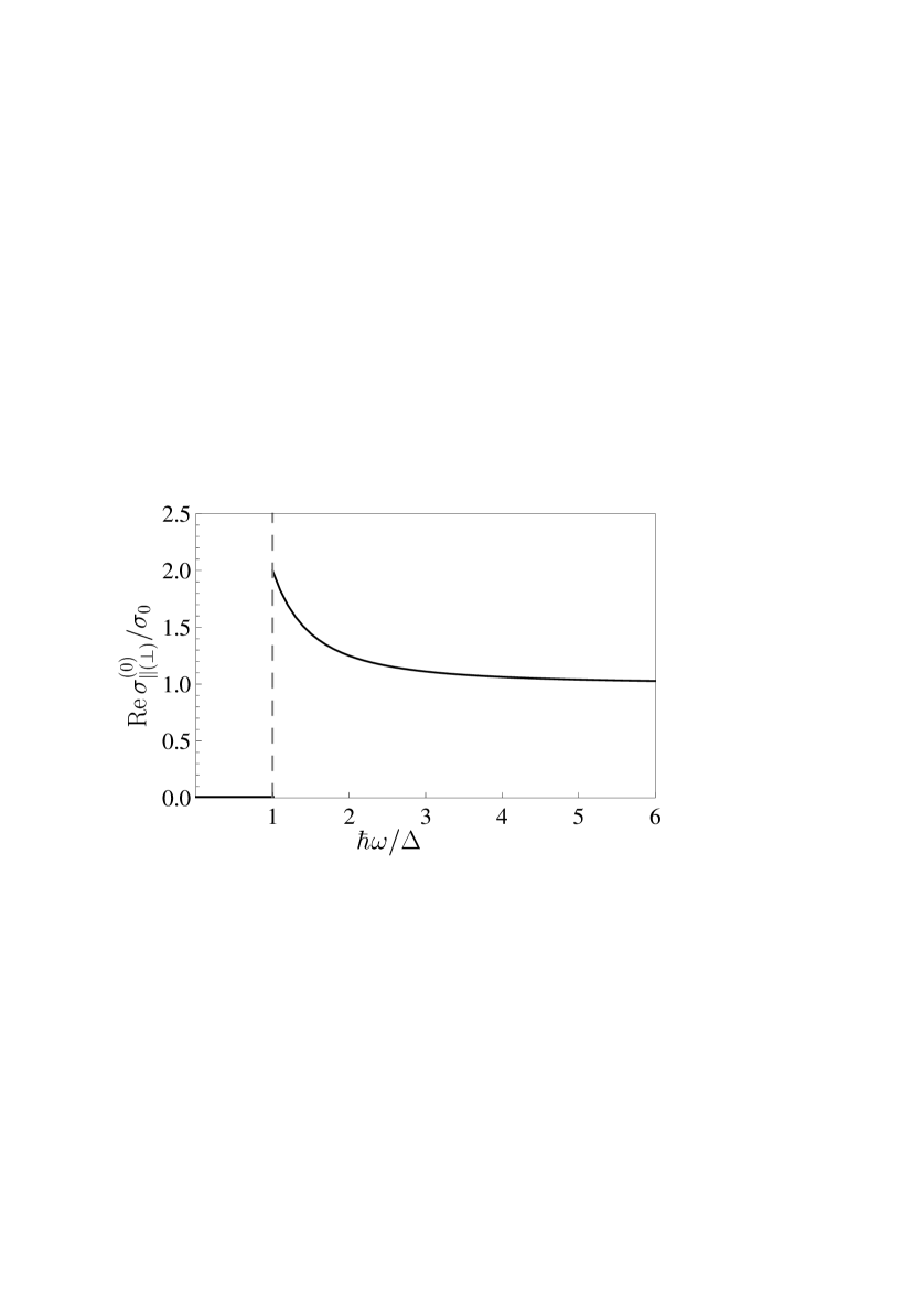
Figure 1: The real part of the conductivity of gapped graphene at zero temperature normalized to $\sigma_{0}$ is shown by the solid line as a function of frequency divided by the width of the gap. The dashed line illustrates the condition $\hbar\omega=\Delta$.

As is seen from Eq. (20), ${\rm Re}\sigma_{\|}$ and ${\rm Re}\sigma_{\bot}$ differ only in the first perturbation order in the small parameter (19) and, thus, can be considered as equal for all practical purposes. They are normalized to $\sigma_{0}$ and plotted in Fig. 1 as functions of $\hbar\omega/\Delta$. Note that in this and all the following figures computational results for the longitudinal and transverse conductivities are indistinguishable in the used scales. Because of this, they are always presented by a single line. In the region $\hbar\omega\geq\Delta$ the conductivities of graphene are the monotonous functions decreasing from $2\sigma_{0}$ to $\sigma_{0}$ when the frequency increases from $\Delta/\hbar$ to infinity.

In the local limit, where the results are independent on the wave vector, Eq. (20) leads to

$${\rm Re}\sigma_{\|}^{(0)}(\omega,0)={\rm Re}\sigma_{\bot}^{(0)}(\omega,0)=\sigma_{0}\frac{(\hbar\omega)^{2}+\Delta^{2}}{(\hbar\omega)^{2}}\theta(\hbar\omega-\Delta).$$ (21)

Note that in our case the same results are obtained from Eq. (20) taken at $k=0$. They coincide with the results presented in Ref. 27 obtained in the framework of another approach.

III.2 Imaginary part of conductivity

Using Eq. (14), for the imaginary part of conductivity of graphene at zero temperature we obtain

$${\rm Im}\sigma_{\|}^{(0)}(\omega,k)=-\frac{\omega}{4\pi\hbar k^{2}}{\rm Re}\Pi_{00}^{(0)}(\omega,k),$$ (22)

$${\rm Im}\sigma_{\bot}^{(0)}(\omega,k)=\frac{c^{2}}{4\pi\hbar k^{2}\omega}{\rm Re}\Pi^{(0)}(\omega,k).$$

For the real part of the polarization tensor from Eqs. (3)–(5) one finds

$${\rm Re}\Pi_{00}^{(0)}(\omega,k)=-\frac{\alpha k^{2}c^{2}}{\omega^{2}\eta^{2}}{\rm Re}\Phi(\omega,k),$$

$${\rm Re}\Pi^{(0)}(\omega,k)=\alpha k^{2}{\rm Re}\Phi(\omega,k),$$ (23)

where

$${\rm Re}\Phi(\omega,k)=\frac{2\Delta}{c}-\frac{2\hbar\omega\eta}{c}\left[1+\left(\frac{\Delta}{\hbar\omega\eta}\right)^{\!\!2}\right]\left\{\begin{array}[]{ll}{\rm arctanh}\frac{\hbar\omega\eta}{\Delta},&\hbar\omega\eta<\Delta,\\ {\rm arctanh}\frac{\Delta}{\hbar\omega\eta},&\hbar\omega\eta\geq\Delta.\end{array}\right.$$ (24)

Using the identity 63

$${\rm arctanh}z=\frac{1}{2}\ln\frac{1+z}{1-z},$$ (25)

Eq. (24) can be rewritten in the form

$${\rm Re}\Phi(\omega,k)=\frac{2\Delta}{c}-\frac{\hbar\omega\eta}{c}\left[1+\left(\frac{\Delta}{\hbar\omega\eta}\right)^{\!\!2}\right]\ln\left|\frac{\Delta+\hbar\omega\eta}{\Delta-\hbar\omega\eta}\right|.$$ (26)

Substituting Eqs. (23) and (26) in Eq. (22), one arrives at

$${\rm Im}\sigma_{\|}^{(0)}(\omega,k)=\frac{\sigma_{0}}{\pi\eta}\left[\frac{2\Delta}{\hbar\omega\eta}-\frac{(\hbar\omega\eta)^{2}+\Delta^{2}}{(\hbar\omega\eta)^{2}}\ln\left|\frac{\Delta+\hbar\omega\eta}{\Delta-\hbar\omega\eta}\right|\right],$$

(27)

$${\rm Im}\sigma_{\bot}^{(0)}(\omega,k)=\frac{\sigma_{0}\eta}{\pi}\left[\frac{2\Delta}{\hbar\omega\eta}-\frac{(\hbar\omega\eta)^{2}+\Delta^{2}}{(\hbar\omega\eta)^{2}}\ln\left|\frac{\Delta+\hbar\omega\eta}{\Delta-\hbar\omega\eta}\right|\right].$$

From Eq. (27) it is seen that the nonlocal effects play equally small role in the imaginary parts of conductivity of graphene as in its real part. In the local limit we have $\eta(\omega,0)=1$ and Eq. (27) reduces to

$${\rm Im}\sigma_{\|}^{(0)}(\omega,0)={\rm Im}\sigma_{\bot}^{(0)}(\omega,0)=\frac{\sigma_{0}}{\pi}\left[\frac{2\Delta}{\hbar\omega}-\frac{(\hbar\omega)^{2}+\Delta^{2}}{(\hbar\omega)^{2}}\ln\left|\frac{\Delta+\hbar\omega}{\Delta-\hbar\omega}\right|\right].$$ (28)

This coincides with the result presented in Ref. 27 .

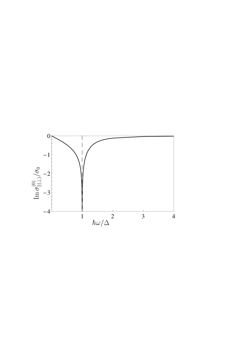
Figure 2: The imaginary part of the conductivity of gapped graphene at zero temperature normalized to $\sigma_{0}$ is shown by the solid line as a function of frequency divided by the width of the gap. The dashed line illustrates the condition $\hbar\omega=\Delta$.

In Fig. 2 we plot the imaginary part of the conductivity of graphene normalized to $\sigma_{0}$ at $T=0$ as a function of the ratio of $\hbar\omega$ to the width of the gap $\Delta$. As is seen in Fig. 2, for any fixed $\Delta$ the imaginary part of conductivity decreases monotonously from zero to minus infinity when frequency increases from 0 to $\Delta/\hbar$ and then increases to zero with further increase of frequency.

IV Real part of conductivity of gapped graphene at nonzero temperature

We start from the real parts of thermal corrections to the conductivities of graphene. According to Eqs. (2) and (14), they are given by

$${\rm Re}\Delta_{T}\sigma_{\|}(\omega,k,T)=\frac{\omega}{4\pi\hbar k^{2}}{\rm Im}\Delta_{T}\Pi_{00}(\omega,k,T),$$ (29)

$${\rm Re}\Delta_{T}\sigma_{\bot}(\omega,k,T)=-\frac{c^{2}}{4\pi\hbar k^{2}\omega}{\rm Im}\Delta_{T}\Pi(\omega,k,T).$$

Recall that the quantities ${\rm Im}\Delta_{T}\Pi_{00}$ and ${\rm Im}\Delta_{T}\Pi$ (and, thus, ${\rm Re}\Delta_{T}\sigma_{\|}$ and ${\rm Re}\Delta_{T}\sigma_{\bot}$) are equal to zero under the condition $\hbar\omega\eta<\Delta$. Under the opposite condition $\hbar\omega\eta\geq\Delta$ they are given by Eq. (6).

It is convenient to introduce another integration variable in Eq. (6)

$$\tau=\frac{2cu-\omega}{v_{F}k\sqrt{A(\omega,k)}},$$ (30)

where $A$ is defined in Eq. (7). Then Eq. (6) takes the form

$${\rm Im}\Delta_{T}\Pi_{00}(\omega,k,T)=-4\alpha\hbar\frac{ck^{2}}{\omega\eta}\int_{-1}^{1}\frac{d\tau}{\exp\left(\frac{\hbar\omega}{2k_{B}T}+\gamma\tau\right)+1}\left[\frac{1-A(\omega,k)}{\sqrt{1-\tau^{2}}}+A(\omega,k)\sqrt{1-\tau^{2}}\right],$$

(31)

$${\rm Im}\Delta_{T}\Pi(\omega,k,T)=4\alpha\hbar\omega\eta\frac{k^{2}}{c}\int_{-1}^{1}\frac{d\tau}{\exp\left(\frac{\hbar\omega}{2k_{B}T}+\gamma\tau\right)+1}\left[\frac{1}{\sqrt{1-\tau^{2}}}-A(\omega,k)\sqrt{1-\tau^{2}}\right].$$

Here, the parameter $\gamma$ is defined as

$$\gamma\equiv\gamma(\omega,k,T)=\frac{v_{F}k}{\omega}\,\frac{\hbar\omega}{2k_{B}T}\sqrt{A(\omega,k)}.$$ (32)

It is equal to zero in the local limit.

Expanding the exponent-containing fraction in the first formula of Eq. (31) in a series and calculating the integrals 63 one obtains

$${\rm Im}\Delta_{T}\Pi_{00}(\omega,k,T)=-4\alpha\hbar\frac{ck^{2}}{\omega\eta}\sum_{n=1}^{\infty}(-1)^{n-1}e^{-\frac{n\hbar\omega}{2k_{B}T}}\int_{-1}^{1}d\tau e^{-n\gamma\tau}\left[\frac{1-A(\omega,k)}{\sqrt{1-\tau^{2}}}+A(\omega,k)\sqrt{1-\tau^{2}}\right]$$

(33)

$$~{}~{}=-4\alpha\hbar\frac{ck^{2}}{\omega\eta}\sum_{n=1}^{\infty}(-1)^{n-1}e^{-\frac{n\hbar\omega}{2k_{B}T}}\left\{\left[1-A(\omega,k)\right]{I}_{0}(n\gamma)+\frac{A(\omega,k)}{n\gamma}{I}_{1}(n\gamma)\right\},$$

where ${I}_{k}(z)$ are the Bessel functions of an imaginary argument.

In a similar manner, the second formula of Eq. (31) can be rewritten as

$${\rm Im}\Delta_{T}\Pi(\omega,k,T)=4\alpha\hbar\omega\eta\frac{k^{2}}{c}\sum_{n=1}^{\infty}(-1)^{n-1}e^{-\frac{n\hbar\omega}{2k_{B}T}}\int_{-1}^{1}d\tau e^{-n\gamma\tau}\left[\frac{1}{\sqrt{1-\tau^{2}}}-A(\omega,k)\sqrt{1-\tau^{2}}\right]$$

(34)

$$~{}~{}~{}~{}~{}~{}=4\alpha\hbar\omega\eta\frac{k^{2}}{c}\sum_{n=1}^{\infty}(-1)^{n-1}e^{-\frac{n\hbar\omega}{2k_{B}T}}\left[{I}_{0}(n\gamma)-\frac{A(\omega,k)}{n\gamma}{I}_{1}(n\gamma)\right].$$

Substituting Eqs. (33) and (34) with added $\theta$-functions in Eq. (29), we obtain the exact expressions for the real parts of thermal corrections to longitudinal and transverse conductivities of gapped graphene at nonzero temperature

$${\rm Re}\Delta_{T}\sigma_{\|}(\omega,k,T)=-\frac{4\sigma_{0}}{\eta}\theta(\hbar\omega\eta-\Delta)\sum_{n=1}^{\infty}(-1)^{n-1}e^{-\frac{n\hbar\omega}{2k_{B}T}}\left\{\left[1-A(\omega,k)\right]{I}_{0}(n\gamma)+\frac{A(\omega,k)}{n\gamma}{I}_{1}(n\gamma)\right\},$$

(35)

$${\rm Re}\Delta_{T}\sigma_{\bot}(\omega,k,T)=-{4\sigma_{0}}{\eta}\theta(\hbar\omega\eta-\Delta)\sum_{n=1}^{\infty}(-1)^{n-1}e^{-\frac{n\hbar\omega}{2k_{B}T}}\left[{I}_{0}(n\gamma)-\frac{A(\omega,k)}{n\gamma}{I}_{1}(n\gamma)\right].$$

To determinate the role of nonlocal effects we expand the right-hand sides of both expressions in Eq. (35) up to the first order in the small parameter (19) and find

$${\rm Re}\Delta_{T}\sigma_{\|}(\omega,k,T)=-\sigma_{0}\theta(\hbar\omega\eta-\Delta)$$

$$\times\left\{2\left[1+\left(\frac{\Delta}{\hbar\omega}\right)^{\!\!2}\right]+\left(\frac{v_{F}k}{\omega}\right)^{\!\!2}\!\left[1+3\left(\frac{\Delta}{\hbar\omega}\right)^{\!\!2}\right]\sum_{n=1}^{\infty}(-1)^{n-1}e^{-\frac{n\hbar\omega}{2k_{B}T}}\right.$$

$$~{}~{}~{}\left.+\frac{1}{4}\left[1-\left(\frac{\Delta}{\hbar\omega}\right)^{\!\!2}\right]\!\left[1+3\left(\frac{\Delta}{\hbar\omega}\right)^{\!\!2}\right]\!\left(\frac{v_{F}k}{\omega}\right)^{\!\!2}\!\left(\frac{\hbar\omega}{2k_{B}T}\right)^{\!\!2}\sum_{n=1}^{\infty}(-1)^{n-1}n^{2}e^{-\frac{n\hbar\omega}{2k_{B}T}}\right\},$$

(36)

$${\rm Re}\Delta_{T}\sigma_{\bot}(\omega,k,T)=-\sigma_{0}\theta(\hbar\omega\eta-\Delta)$$

$$\times\left\{2\left[1+\left(\frac{\Delta}{\hbar\omega}\right)^{\!\!2}\right]-\frac{1}{2}\left(\frac{v_{F}k}{\omega}\right)^{\!\!2}\!\left[1-\left(\frac{\Delta}{\hbar\omega}\right)^{\!\!2}\right]\sum_{n=1}^{\infty}(-1)^{n-1}e^{-\frac{n\hbar\omega}{2k_{B}T}}\right.$$

$$~{}~{}~{}\left.+\frac{1}{4}\left[1-\left(\frac{\Delta}{\hbar\omega}\right)^{\!\!2}\right]\!\left[3+\left(\frac{\Delta}{\hbar\omega}\right)^{\!\!2}\right]\!\left(\frac{v_{F}k}{\omega}\right)^{\!\!2}\!\left(\frac{\hbar\omega}{2k_{B}T}\right)^{\!\!2}\sum_{n=1}^{\infty}(-1)^{n-1}n^{2}e^{-\frac{n\hbar\omega}{2k_{B}T}}\right\}.$$

Performing the summation according to Ref. 63

$$\sum_{n=1}^{\infty}(-1)^{n-1}e^{-\frac{n\hbar\omega}{2k_{B}T}}=\frac{1}{e^{\frac{\hbar\omega}{2k_{B}T}}+1},$$ (37)

$$\sum_{n=1}^{\infty}(-1)^{n-1}n^{2}e^{-\frac{n\hbar\omega}{2k_{B}T}}=\frac{e^{\frac{\hbar\omega}{2k_{B}T}}(e^{\frac{\hbar\omega}{2k_{B}T}}-1)}{(e^{\frac{\hbar\omega}{2k_{B}T}}+1)^{3}},$$

after identical transformations Eq. (36) can be written in the following form:

$${\rm Re}\Delta_{T}\sigma_{\|}(\omega,k,T)=-\frac{2\sigma_{0}\theta(\hbar\omega\eta-\Delta)}{e^{\frac{\hbar\omega}{2k_{B}T}}+1}\left\{\vphantom{\left[\frac{{\rm tanh}\frac{\hbar\omega}{4k_{B}T}}{1+e^{-\frac{\hbar\omega}{2k_{B}T}}}\right]}1+\left(\frac{\Delta}{\hbar\omega}\right)^{\!\!2}+\frac{1}{2}\left(\frac{v_{F}k}{\omega}\right)^{\!\!2}\right.$$

$$~{}~{}~{}\left.\times\left[1+3\left(\frac{\Delta}{\hbar\omega}\right)^{\!\!2}\right]\!\left[1+\frac{(\hbar\omega)^{2}-\Delta^{2}}{16(k_{B}T)^{2}}\frac{{\rm tanh}\frac{\hbar\omega}{4k_{B}T}}{1+e^{-\frac{\hbar\omega}{2k_{B}T}}}\right]\right\},$$

(38)

$${\rm Re}\Delta_{T}\sigma_{\bot}(\omega,k,T)=-\frac{2\sigma_{0}\theta(\hbar\omega\eta-\Delta)}{e^{\frac{\hbar\omega}{2k_{B}T}}+1}\left\{\vphantom{\left[\frac{{\rm tanh}\frac{\hbar\omega}{4k_{B}T}}{1+e^{-\frac{\hbar\omega}{2k_{B}T}}}\right]}1+\left(\frac{\Delta}{\hbar\omega}\right)^{\!\!2}-\frac{1}{2}\left(\frac{v_{F}k}{\omega}\right)^{\!\!2}\right.$$

$$~{}~{}~{}\left.\times\left[1-\left(\frac{\Delta}{\hbar\omega}\right)^{\!\!2}\right]\!\left[1-\frac{3(\hbar\omega)^{2}+\Delta^{2}}{16(k_{B}T)^{2}}\frac{{\rm tanh}\frac{\hbar\omega}{4k_{B}T}}{1+e^{-\frac{\hbar\omega}{2k_{B}T}}}\right]\right\}.$$

As is seen from Eq. (38), the real parts of thermal corrections to the conductivity of gapped graphene are mostly determined by the local contributions

$${\rm Re}\Delta_{T}\sigma_{\|}(\omega,0,T)={\rm Re}\Delta_{T}\sigma_{\bot}(\omega,0,T)=-\frac{2\sigma_{0}}{e^{\frac{\hbar\omega}{2k_{B}T}}+1}\frac{(\hbar\omega)^{2}+\Delta^{2}}{(\hbar\omega)^{2}}\theta(\hbar\omega-\Delta).$$ (39)

The nonlocal contributions in Eq. (38) become dominant only at very low temperature when the complete thermal correction is exponentially small.

By adding Eqs. (21) and (39), one arrives at the final expression for the real part of conductivity of gapped graphene at nonzero temperature in the local approximation

$${\rm Re}\sigma_{\|(\bot)}(\omega,0,T)=\sigma_{0}{\rm tanh}\frac{\hbar\omega}{4k_{B}T}\frac{(\hbar\omega)^{2}+\Delta^{2}}{(\hbar\omega)^{2}}\theta(\hbar\omega\eta-\Delta).$$ (40)

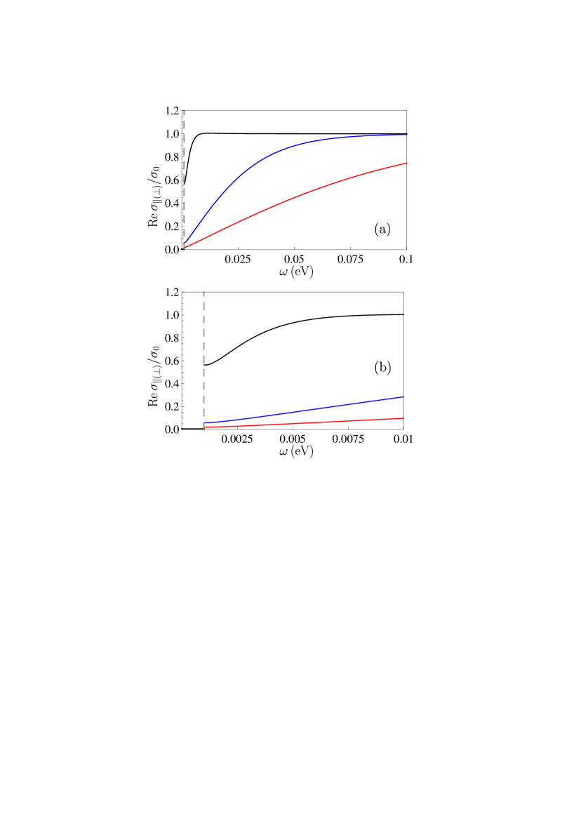
Figure 3: (a) The normalized to $\sigma_{0}$ real part of the conductivity of graphene with the gap parameter $\Delta=0.001\,$eV is shown as a function of frequency by the three lines plotted from top to bottom at temperature $T=10$, 100, and 300 K, respectively. The dashed line illustrates the condition $\hbar\omega=\Delta$. (b) The same is shown on an enlarged scale at low frequencies.

In Fig. 3(a) we plot the real part of the normalized to $\sigma_{0}$ longitudinal and transverse conductivities of graphene with the gap parameter $\Delta=0.001\,$eV as a function of frequency (measured in eV) at different temperatures. The lines from top to bottom correspond to $T=10$, 100, and 300 K, respectively (note that $T=300\,$K corresponds to $k_{B}T\approx 0.025\,$eV). To gain a better understanding, the region of very low frequencies is shown in Fig. 3(b) on an enlarged scale. According to Fig. 3(a,b), the real part of conductivity decreases with increasing $T$. This is because the thermal correction to conductivity presented in Eq. (39) is negative. As is seen in Fig. 3(a,b), the real part of the conductivity of graphene increases with increasing frequency and goes to $\sigma_{0}$. This is, however, not a universal property, but is determined by chosen (small) value of the gap parameter.

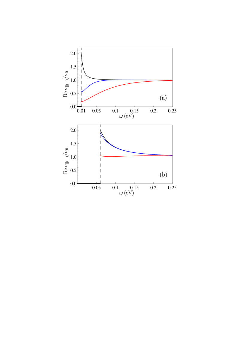
Figure 4: The normalized to $\sigma_{0}$ real part of the conductivity of graphene with the gap parameter (a) $\Delta=0.01\,$eV and (b) $\Delta=0.06\,$eV is shown as a function of frequency by the three lines plotted from top to bottom at temperature $T=10$, 100, and 300 K, respectively. The dashed line illustrates the condition $\hbar\omega=\Delta$.

To illustrate the latter statement, In Fig. 4 we plot the real parts of the conductivities of graphene with the larger gap parameters equal to (a) $\Delta=0.01\,$eV and (b) $\Delta=0.06\,$eV as the functions of frequency. The lines from top to bottom are plotted for $T=10$, 100, and 300 K, respectively. As is seen in Fig. 4(a), at $T=300$ and 100 K the real part of conductivity increases, but at $T=10\,$K it decreases with increasing frequency. Figure 4(b) illustrates what is happening with an increase of the gap parameter to $\Delta=0.06\,$eV. In this case the real part of conductivity at $T=10$ and 100 K decreases with increasing frequency, whereas at $T=300\,$K it becomes nonmonotonous due to an interplay of two factors in Eq. (40). With further increase of the gap parameter (up to $\Delta=0.1\,$eV or larger) the real part of conductivity becomes monotonously decreasing at all considered temperatures, whereas the values of ${\rm Re}\sigma_{\|(\bot)}$ at $T=10$ and 100 K become indistinguishable.

V Imaginary part of conductivity of gapped graphene at nonzero temperature

The imaginary parts of thermal corrections to the conductivity of graphene are obtained from Eqs. (2) and (14)

$${\rm Im}\Delta_{T}\sigma_{\|}(\omega,k,T)=-\frac{\omega}{4\pi\hbar k^{2}}{\rm Re}\Delta_{T}\Pi_{00}(\omega,k,T),$$ (41)

$${\rm Im}\Delta_{T}\sigma_{\bot}(\omega,k,T)=\frac{c^{2}}{4\pi\hbar k^{2}\omega}{\rm Re}\Delta_{T}\Pi(\omega,k,T).$$

At first we consider the frequency region $\hbar\omega\eta<\Delta$. Here, the real parts of the temperature corrections to the polarization tensor are presented by Eq. (9). Thus, the exact expressions for ${\rm Im}\Delta_{T}\sigma_{\|}$ and ${\rm Im}\Delta_{T}\sigma_{\bot}$ in this region are given by Eqs. (9) and (41). The total imaginary part of the conductivity is given by

$${\rm Im}\sigma_{\|(\bot)}(\omega,k,T)={\rm Im}\sigma_{\|(\bot)}^{(0)}(\omega,k)+{\rm Im}\Delta_{T}\sigma_{\|(\bot)}(\omega,k,T),$$ (42)

where ${\rm Im}\sigma_{\|(\bot)}^{(0)}$ is defined in Eq. (27).

We expand Eq. (9) up to the first order in a small parameter (19) and find

$${\rm Re}\Delta_{T}\Pi_{00}(\omega,k,T)=-\frac{8\alpha\hbar c^{2}k^{2}}{\omega^{2}}\int_{\Delta/(2\hbar c)}^{\infty}\frac{du}{e^{\beta u}+1}\left[1+\frac{\Delta^{2}+(\hbar\omega)^{2}}{4(\hbar cu)^{2}-(\hbar\omega)^{2}}\right],$$

(43)

$${\rm Re}\Delta_{T}\Pi(\omega,k,T)=8\alpha\hbar k^{2}\int_{\Delta/(2\hbar c)}^{\infty}\frac{du}{e^{\beta u}+1}\left[1+\frac{\Delta^{2}+(\hbar\omega)^{2}}{4(\hbar cu)^{2}-(\hbar\omega)^{2}}\right].$$

Substituting these equations in Eq. (41), one arrives at equal results for ${\rm Im}\Delta_{T}\sigma_{\|}$ and ${\rm Im}\Delta_{T}\sigma_{\bot}$ in the local approximation

$${\rm Im}\Delta_{T}\sigma_{\|(\bot)}(\omega,0,T)=\frac{8\sigma_{0}c}{\pi\omega}\int_{\Delta/(2\hbar c)}^{\infty}\frac{du}{e^{\beta u}+1}\left[1+\frac{\Delta^{2}+(\hbar\omega)^{2}}{4(\hbar cu)^{2}-(\hbar\omega)^{2}}\right].$$ (44)

Similar to Sec. IV, it can be shown that the nonlocal corrections to ${\rm Im}\Delta_{T}\sigma_{\|(\bot)}(\omega,0,T)$ are negligibly small.

The total imaginary part of the conductivity of graphene in the local approximation is given by

$${\rm Im}\sigma_{\|(\bot)}(\omega,0,T)={\rm Im}\sigma_{\|(\bot)}^{(0)}(\omega,0)+{\rm Im}\Delta_{T}\sigma_{\|(\bot)}(\omega,0,T),$$ (45)

where ${\rm Im}\sigma_{\|(\bot)}^{(0)}$ and ${\rm Im}\Delta_{T}\sigma_{\|(\bot)}$ are given by Eqs. (28) and (44), respectively.

Note that under the condition $\Delta\ll k_{B}T$ we can obtain simple asymptotic expression for ${\rm Im}\Delta_{T}\sigma_{\|(\bot)}$ in Eq. (44). For this purpose we take into account that the main contribution to the integral is given by $u\approx 1/\beta=k_{B}T/(\hbar c)$ and that the condition $\Delta\ll k_{B}T$ in the frequency region under consideration leads to $\hbar\omega<\Delta\ll k_{B}T$ as well. Then, one can neglect by the second term in square brackets of Eq. (44) as compared to unity and, after the integration, arrive at

$${\rm Im}\Delta_{T}\sigma_{\|(\bot)}(\omega,0,T)\approx 8\sigma_{0}\frac{k_{B}T}{\pi\hbar\omega}\ln\left(1+e^{-\frac{\Delta}{2k_{B}T}}\right)\approx 8\sigma_{0}\frac{k_{B}T}{\pi\hbar\omega}\ln 2.$$ (46)

As is seen from Eqs. (28) and (44), the imaginary part of the conductivity of gapped graphene is negative, whereas the thermal correction to it is positive. This means that the total imaginary part of the conductivity may change its sign at some frequency. Numerical computations confirm this conclusion.

We have computed ${\rm Im}\sigma_{\|(\bot)}$ normalized to $\sigma_{0}$ as a function of $\omega$ in the region $\hbar\omega<\Delta$ at room temperature $T=300\,$K in two ways: by Eqs. (9), (27), (41), and (42), i.e., using the exact polarization tensor with several selected values of $k$, and by Eqs. (28), (44), and (45), i.e., in the local approximation, with nearly coincident results. In Fig. 5(a) the normalized imaginary part of conductivity of graphene with the gap parameter $\Delta=0.02\,$eV is shown as a function of frequency in the region $\hbar\omega<\Delta$ (the latter is marked by the vertical dashed line). As is seen in Fig. 5(a), ${\rm Im}\sigma_{\|(\bot)}$ varies from infinity at zero frequency to minus infinity when $\hbar\omega\to\Delta$. It has a root at some $\hbar\omega$ close to $\Delta$. For better vizualization, in Fig. 5(b) we show an immediate vicinity of the frequency $\omega=\Delta/\hbar$ on an enlarged scale. The root of ${\rm Im}\sigma_{\|(\bot)}$ is $\hbar\omega_{0}=0.019525\,$eV. The behavior of ${\rm Im}\Delta_{T}\sigma_{\|(\bot)}$ at $\omega=0$ is determined by the thermal correction ${\rm Im}\Delta_{T}\sigma_{\|(\bot)}$, whereas the behavior in the limiting case $\hbar\omega\to\Delta$ is caused by the imaginary part of conductivity at zero temperature ${\rm Im}\sigma_{\|(\bot)}^{(0)}$ (compare with Fig. 2).

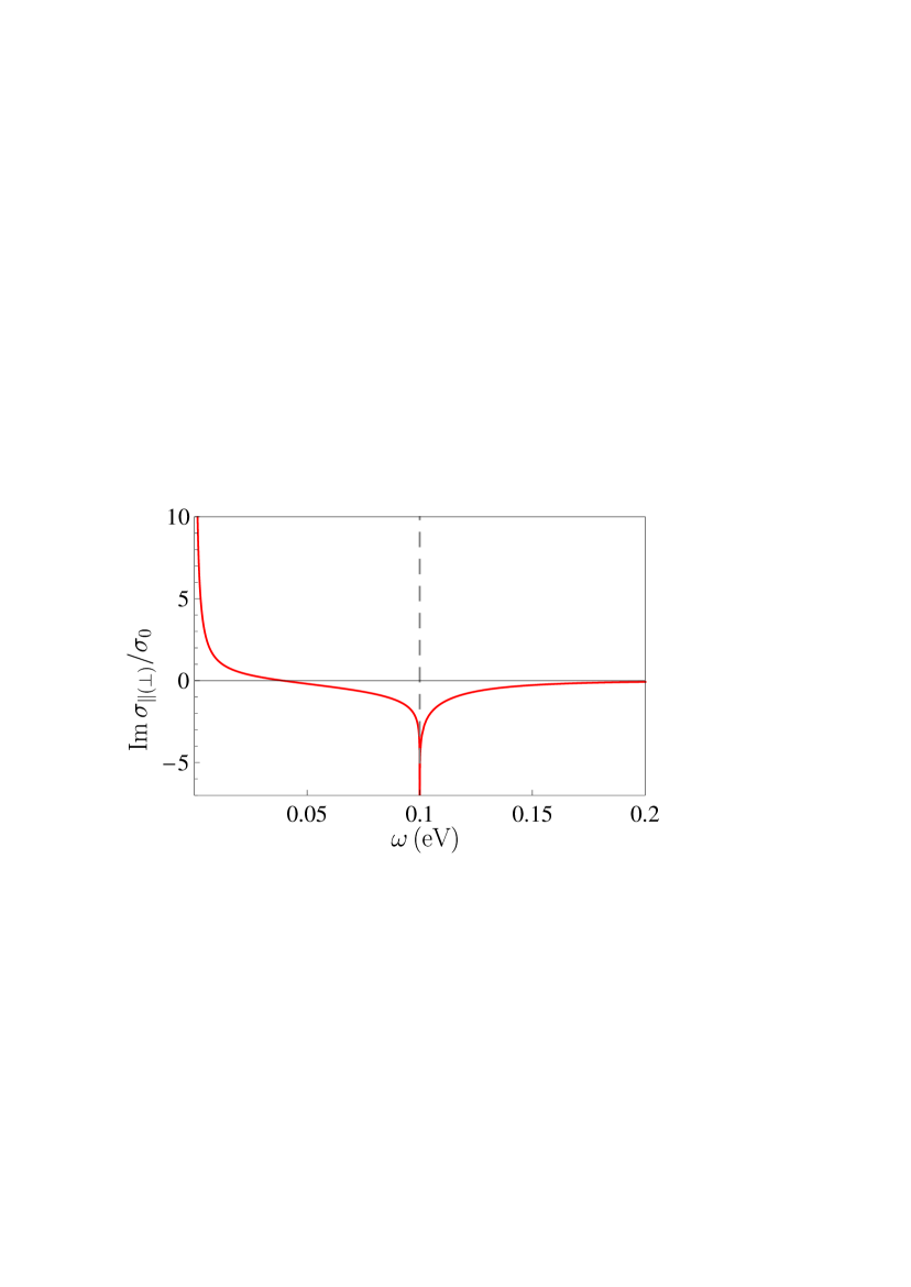
Figure 6: The normalized to $\sigma_{0}$ imaginary part of the conductivity of graphene with the gap parameter $\Delta=0.1\,$eV is shown as a function of frequency by the solid line plotted at temperature $T=300\,$K. The dashed line illustrates the condition $\hbar\omega=\Delta$.

For comparison purposes, in Fig. 6 the computational results for ${\rm Im}\sigma_{\|(\bot)}$ at $T=300\,$K, $\hbar\omega<\Delta$ are shown also for a larger gap $\Delta=0.1\,$eV. As is seen in Fig. 6, in this case the root of ${\rm Im}\sigma_{\|(\bot)}$, $\hbar\omega_{0}=0.03923\,$eV, is much more separated from the border frequency $\hbar\omega=\Delta$ than in Fig. 5 (see below for the discussion of the frequency region $\hbar\omega\geq\Delta$).

We are coming now to the imaginary parts of the conductivities of graphene ${\rm Im}\sigma_{\|(\bot)}$ under the condition $\hbar\omega\geq\Delta$. The imaginary parts of the thermal corrections, ${\rm Im}\Delta_{T}\sigma_{\|(\bot)}$, are again given by Eq. (41) where, however, the quantities ${\rm Re}\Delta_{T}\Pi_{00}$ and ${\rm Re}\Delta_{T}\Pi$ are expressed by Eqs. (10)–(13). These expressions, together with the contribution at zero temperature in Eq. (27), are used below in numerical computations.

It is possible also to obtain the asymptotic expressions valid under certain additional conditions. Thus, according to Ref. 56 , at relatively high frequencies satisfying the condition $\hbar\omega\gg k_{B}T\gg\Delta$ one obtains

$${\rm Re}\Delta_{T}\Pi_{00}(\omega,k,T)\approx 48\alpha k^{2}\frac{(k_{B}T)^{3}}{(\hbar\omega)^{2}}\,\frac{c}{\omega^{2}}\zeta(3),$$

$${\rm Re}\Delta_{T}\Pi(\omega,k,T)\approx-48\alpha\frac{k^{2}}{c}\,\frac{(k_{B}T)^{3}}{(\hbar\omega)^{2}}\zeta(3),$$ (47)

where $\zeta(z)$ is the Riemann zeta function.

Substituting these equations in Eq. (41), we have

$${\rm Im}\Delta_{T}\sigma_{\|(\bot)}(\omega,0,T)\approx-\frac{48\zeta(3)}{\pi}\sigma_{0}\left(\frac{k_{B}T}{\hbar\omega}\right)^{3}.$$ (48)

If $\hbar\omega\gg k_{B}T$ and $\Delta\gg k_{B}T$ the following asymptotic expressions are valid 56

$${\rm Re}\Delta_{T}\Pi_{00}(\omega,k,T)\approx 24\alpha\frac{k_{B}T}{(\hbar\omega)^{2}}\,\frac{k^{2}c\Delta^{2}}{\omega^{2}}e^{-\frac{\Delta}{2k_{B}T}},$$

$${\rm Re}\Delta_{T}\Pi(\omega,k,T)\approx-24\alpha\frac{k_{B}T}{(\hbar\omega)^{2}}\,\frac{k^{2}\Delta^{2}}{c}e^{-\frac{\Delta}{2k_{B}T}}.$$ (49)

Then from Eq. (41) one arrives at

$${\rm Im}\Delta_{T}\sigma_{\|(\bot)}(\omega,0,T)\approx-\frac{24}{\pi}\sigma_{0}\frac{k_{B}T}{(\hbar\omega)^{3}}\Delta^{2}e^{-\frac{\Delta}{2k_{B}T}}.$$ (50)

The complete imaginary part of the conductivity of gapped graphene under respective conditions is obtained by summing Eqs. (48) and (50) with Eq. (28).

Now we present the results of numerical computations using the exact formulas (10)–(13), (27), and (41). In Figs. 5(a) and 5(b) the computational results for ${\rm Im}\sigma_{\|(\bot)}$ normalized to $\sigma_{0}$ are presented in the frequency region $\hbar\omega>\Delta=0.02\,$eV at room temperature $T=300\,$K. In Fig. 6 similar results are shown for graphene with the gap parameter $\Delta=0.1\,$eV. As is seen in Figs. 5(a,b) and 6, in the frequency region $\hbar\omega>\Delta$ the imaginary part of $\sigma_{\|(\bot)}$ varies from minus infinity to zero with increasing frequency, i.e., qualitatively in the same way as at zero temperature. By comparing Figs. 5(a) and 6 it is seen that for a larger gap parameter ${\rm Im}\sigma_{\|(\bot)}$ faster approaches to zero with increasing frequency. It can be seen that Fig. 6 in the frequency region $\hbar\omega>\Delta$ is in a rather good agreement with the asymptotic expression (50) added to the zero-temperature contribution (28). This is in accordance with the application conditions of Eq. (50).

VI Conclusions and discussion

In the foregoing, we have investigated the conductivity of gapped graphene described by the Dirac model on the basis of first principles of quantum electrodynamics. In doing so, no input parameter has been used. Both cases of zero and nonzero temperature have been considered. The longitudinal and transverse conductivities of graphene were expressed via the components of the polarization tensor in (2+1)-dimensional space-time valid over the entire plane of complex frequency 54 . This is a microscopic description in the sense that the polarization tensor eventually represents the response of individual electronic excitations to the electromagnetic field.

At zero temperature, we have confirmed the analytic expressions (21) and (28) for both real and imaginary parts of the conductivity of graphene obtained earlier in the local approximation 27 . We have also generalized these expressions in Eqs. (17) and (27) taking into account nonlocal effects.

The exact expressions for the real parts of thermal corrections to the real parts of conductivities of gapped graphene at zero temperature are defined in Eq. (35). The small role of nonlocal effects is demonstrated in Eq. (38). Finally, simple analytic expression for the real part of the total conductivity of gapped graphene at any temperature is given by Eq. (40). According to our results, the real part of conductivity is equal to zero for $\hbar\omega<\Delta$. In the frequency region $\hbar\omega\geq\Delta$ the real part of conductivity takes some value $\sigma^{\ast}$ belonging to the interval $(0,2\sigma_{0})$ at $\hbar\omega=\Delta$ and goes to $\sigma_{0}$ with increasing frequency. The value $\sigma^{\ast}$ depends on the values of the temperature and gap parameter.

For the imaginary parts of thermal corrections to the imaginary parts of conductivities of gapped graphene at zero temperature, the exact expressions are obtained in Eqs. (41) and (9) in the frequency region $\hbar\omega\eta<\Delta$. In the local approximation, the simple Eq. (44) is obtained, as well as the asymptotic expression (46). The most important impact of temperature on the imaginary part of conductivity of gapped graphene is that it goes to infinity when the frequency vanishes (at $T=0$ the imaginary part of conductivity goes to zero with vanishing frequency).

In the frequency region $\hbar\omega\eta\geq\Delta$ the exact expressions for the imaginary parts of thermal corrections are given by Eqs. (41) and (10)–(13). The simple asymptotic expressions in this case are given in Eqs. (48) and (50). In all cases, the results of numerical computations performed using the exact formulas are in a very good agreement with that using the local approximation and with the asymptotic expansions in their areas of application. In the limiting case $\Delta\to 0$ all the results of this paper smoothly transform into the previously obtained ones for pure graphene 58 .

Finally, we conclude that the description of graphene by means of the polarization tensor calculated using the first principles of quantum electrodynamics at nonzero temperature in (2+1)-dimensional space-time turns out to be very fruitful not only in the Casimir effect, but also for a better understanding of more conventional physical phenomena, such as the reflectivity and conductivity properties of graphene. In this respect it would be interesting to apply the results of the recent Ref. 64 for theoretical description of electrical conductivity of graphene with nonzero chemical potential using the formalism of the polarization tensor.

                      

     

                      

                      

                      

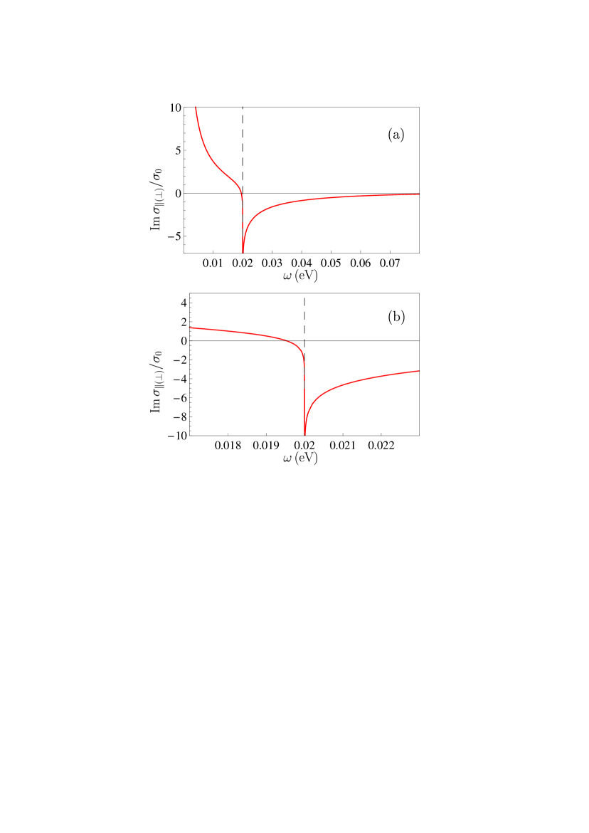
Figure 5: (a) The normalized to $\sigma_{0}$ imaginary part of the conductivity of graphene with the gap parameter $\Delta=0.02\,$eV is shown as a function of frequency by the solid line plotted at temperature $T=300\,$K. The dashed line illustrates the condition $\hbar\omega=\Delta$. (b) The same is shown on an enlarged scale in the vicinity of $\hbar\omega=\Delta$.

References

- (1) M. I. Katsnelson, Graphene: Carbon in Two Dimensions (Cambridge University Press, Cambridge, 2012).
- (2) A. H. Castro Neto, F. Guinea, N. M. R. Peres, K. S. Novoselov, and A. K. Geim, Rev. Mod. Phys. 81, 109 (2009).
- (3) N. M. R. Peres, Rev. Mod. Phys. 82, 2673 (2010).
- (4) S. Das Sarma, S. Adam, E. H. Hwang, and E. Rossi, Rev. Mod. Phys. 83, 407 (2011).
- (5) A. W. W. Ludwig, M. P. A. Fisher, R. Shankar, and G. Grinstein, Phys. Rev. B 50, 7526 (1994).
- (6) T. Ando, Y. Zheng, and H. Suzuura, J. Phys. Soc. Jpn. 71, 1318 (2002).
- (7) V. P. Gusynin and S. G. Sharapov, Phys. Rev. B 73, 245411 (2006).
- (8) M. I. Katsnelson, Eur. Phys. J. B 51, 157 (2006).
- (9) K. Ziegler, Phys. Rev. Lett. 97, 266802 (2006).
- (10) K. Ziegler, Phys. Rev. B 75, 233407 (2007).
- (11) V. P. Gusynin, S. G. Sharapov, and J. P. Carbotte, Phys. Rev. Lett. 98, 157402 (2007).
- (12) M. Trushin and J. Schliemann, Phys. Rev. Lett. 99, 216602 (2007).
- (13) L. A. Falkovsky and A. A. Varlamov, Eur. Phys. J. B 56, 281 (2007).
- (14) L. A. Falkovsky and S. S. Pershoguba, Phys. Rev. B 76, 153410 (2007).
- (15) M. Auslender and M. I. Katsnelson, Phys. Rev. B 76, 235425 (2007).
- (16) V. P. Gusynin and S. G. Sharapov, J. Phys.: Condens. Matter 19, 026222 (2007).
- (17) V. P. Gusynin, S. G. Sharapov, and J. P. Carbotte, Int. J. Mod. Phys. B 21, 4611 (2007).
- (18) T. Stauber, N. M. R. Peres, and A. K. Geim, Phys. Rev. B 78, 085432 (2008).
- (19) N. M. R. Peres and T. Stauber, Int. J. Mod. Phys. B 22, 2529 (2008).
- (20) T. G. Pedersen, A.-P. Jauho, and K. Pedersen, Phys. Rev. B 79, 113406 (2009).
- (21) M. Lewkowicz and B. Rosenstein, Phys. Rev. Lett. 102, 106802 (2009).
- (22) J. J. Palacios, Phys. Rev. B 82, 165439 (2010).
- (23) L. Moriconi and D. Niemeyer, Phys. Rev. B 84, 193401 (2011).
- (24) P. V. Buividovich, E. V. Luschevskaya, O. V. Pavlovsky, M. I. Polikarpov, and M. V. Ulybyshev, Phys. Rev. B 86, 045107 (2012).
- (25) Á. Bácsi and A. Virosztek, Phys. Rev. B 87, 125425 (2013).
- (26) C. A. Dartora and G. G. Cabrera, Phys. Rev. B 87, 165416 (2013).
- (27) T. Stauber, J. Phys.: Condens. Matter 26, 123201 (2014).
- (28) T. Louvet, P. Delplace, A. A. Fedorenko, and D. Carpentier, Phys. Rev. B 92, 155116 (2015).
- (29) D. K. Patel, A. C. Sharma, and S. S. Z. Ashraf, Phys. Status Solidi 252, 282 (2015).
- (30) M. Merano, Phys. Rev. A 93, 013832 (2016).
- (31) Y.-W. Tan, Y. Zhang, K. Bolotin, Y. Zhao, S. Adam, E. H. Hwang, S. Das Sarma, H. L. Stormer, and P. Kim, Phys. Rev. Lett. 99, 246803 (2007).
- (32) R. R. Nair, P. Blake, A. N. Grigorenko, K. S. Novoselov, T. J. Booth, T. Stauber, N. M. R. Peres, and A. K. Geim, Science 320, 1308 (2008).
- (33) Z. Li, E. Henriksen, Z. Jiang, Z. Hao, M. Martin, P. Kim, H. Stormer, and D. Basov, Nature Phys. 4, 532 (2008).
- (34) K. F. Mak, M. Y. Sfeir, Y. Wu, C. H. Lui, J. A. Misewich, and T. F. Heinz, Phys. Rev. Lett. 101, 196405 (2008).
- (35) J. Horng, C.-F. Chen, B. Geng et al., Phys. Rev. B 83, 165113 (2011).
- (36) M. Bordag, I. V. Fialkovsky, D. M. Gitman, and D. V. Vassilevich, Phys. Rev. B 80, 245406 (2009).
- (37) I. V. Fialkovsky, V. N. Marachevsky, and D. V. Vassilevich, Phys. Rev. B 84, 035446 (2011).
- (38) G. L. Klimchitskaya, U. Mohideen, and V. M. Mostepanenko, Rev. Mod. Phys. 81, 1827 (2009).
- (39) M. Bordag, G. L. Klimchitskaya, U. Mohideen, and V. M. Mostepanenko, Advances in the Casimir Effect (Oxford University Press, Oxford, 2015).
- (40) M. Bordag, G. L. Klimchitskaya, and V. M. Mostepanenko, Phys. Rev. B 86, 165429 (2012).
- (41) M. Chaichian, G. L. Klimchitskaya, V. M. Mostepanenko, and A. Tureanu, Phys. Rev. A 86, 012515 (2012).
- (42) G. L. Klimchitskaya and V. M. Mostepanenko, Phys. Rev. B 87, 075439 (2013).
- (43) G. L. Klimchitskaya, U. Mohideen, and V. M. Mostepanenko, Phys. Rev B 89, 115419 (2014).
- (44) G. L. Klimchitskaya, V. M. Mostepanenko, and Bo E. Sernelius, Phys. Rev. B 89, 125407 (2014).
- (45) B. Arora, H. Kaur, and B. K. Sahoo, J. Phys. B 47, 155002 (2014).
- (46) K. Kaur, J. Kaur, B. Arora, and B. K. Sahoo, Phys. Rev. B 90, 245405 (2014).
- (47) G. L. Klimchitskaya and V. M. Mostepanenko, Phys. Rev. B 91, 045412 (2015).
- (48) G. Gómez-Santos, Phys. Rev. B 80, 245424 (2009).
- (49) D. Drosdoff and L. M. Woods, Phys. Rev. B 82, 155459 (2010).
- (50) D. Drosdoff and L. M. Woods, Phys. Rev. A 84, 062501 (2011).
- (51) Bo E. Sernelius, Europhys. Lett. 95, 57003 (2011).
- (52) Bo E. Sernelius, Phys. Rev. B 85, 195427 (2012).
- (53) A. D. Phan, L. M. Woods, D. Drosdoff, I. V. Bondarev, and N. A. Viet, Appl. Phys. Lett. 101, 113118 (2012).
- (54) G. L. Klimchitskaya and V. M. Mostepanenko, Phys. Rev A 89, 052512 (2014).
- (55) A. A. Banishev, H. Wen, J. Xu, R. K. Kawakami, G. L. Klimchitskaya, V. M. Mostepanenko, and U. Mohideen, Phys. Rev. B 87, 205433 (2013).
- (56) M. Bordag, G. L. Klimchitskaya, V. M. Mostepanenko, and V. M. Petrov, Phys. Rev. D 91, 045037 (2015); 93, 089907(E) (2016).
- (57) G. L. Klimchitskaya and V. M. Mostepanenko, Phys. Rev B 91, 174501 (2015).
- (58) G. L. Klimchitskaya, Int. J. Mod. Phys. A 31, 1641026 (2016).
- (59) G. L. Klimchitskaya, C. C. Korikov, and V. M. Petrov, Phys. Rev. B 92, 125419 (2015); 93, 159906(E) (2016).
- (60) G. L. Klimchitskaya and V. M. Mostepanenko, Phys. Rev B 93, 245419 (2016).
- (61) G. L. Klimchitskaya and V. M. Mostepanenko, Phys. Rev A 93, 052106 (2016).
- (62) P. K. Pyatkovsky, J. Phys.: Condens. Matter 21, 025506 (2009).
- (63) V. P. Gusynin, S. G. Sharapov, and J. P. Carbotte, New J. Phys. 11, 095013 (2009).
- (64) S. A. Jafari, J. Phys.: Condens. Matter 24, 205802 (2012).
- (65) Bo E. Sernelius, J. Phys.: Condens. Matter 27, 214017 (2015).
- (66) I. S. Gradshtein and I. M. Ryzhik, Table of Integrals, Series and Products (Academic Press, New York, 1980).
- (67) M. Bordag, I. Fialkovsky, and D. Vassilevich, Phys. Rev. B 93, 075414 (2016).