Thermodynamics and Superradiant Phase Transitions in a three-level Dicke Model

Abstract

We analyse the thermodynamic properties of a generalised Dicke model, i. e. a collection of three-level systems interacting with two bosonic modes. We show that at finite temperatures the system undergoes first-order phase transitions only, which is in contrast to the zero-temperature case where a second-order phase transition exist as well. We discuss the free energy and prominent expectation values. The limit of vanishing temperature is discussed as well.

I Introduction

The Dicke superradiance model Dicke (1954) as a test-bed for mean-field like phase transitions Hepp and Lieb (1973a) has received renewed attention recently, in particular due to its successful implementation in cold-atom experiments Baumann et al. (2010, 2011); Ritsch et al. (2013); Hamner et al. (2014); Klinder et al. (2015) and optical setups of cavities and lasers Dimer et al. (2007); Baden et al. (2014). Much progress has been made towards a realistic description of non-equilibrium and dissipation Keeling et al. (2010); Nagy et al. (2011); Öztop et al. (2012); Bhaseen et al. (2012); Kónya et al. (2012); Torre et al. (2013); Kopylov et al. (2013); Genway et al. (2014); Dalla Torre et al. (2016); Gelhausen et al. (2016), multi-mode effects Konya et al. (2011), the interplay of the superradiant phase transitions and Bose–Einstein Condensation Piazza et al. (2013), spin glasses Strack and Sachdev (2011), the analysis of interactions Inoue (2012), inhomogeneous couplings Goto and Ichimura (2008); Tsyplyatyev and Loss (2009), finite size effects Vidal and Dusuel (2006), or the adiabatic limit Liberti et al. (2006); Bakemeier et al. (2012). Further extensions of the model have appeared allowing for driving Bastidas et al. (2012); Francica et al. (2016), the creation of Goldstone modes Brandes (2013); Yi-Xiang et al. (2013); Baksic and Ciuti (2014), feedback control Grimsmo et al. (2014); Kopylov et al. (2015), or the transfer to other platforms such as solid-state systems Nataf and Ciuti (2010a, b).

In its simplest version, the Dicke model hosts a mean-field type ground state phase transition (‘quantum bifurcation’) at zero temperature Hepp and Lieb (1973a); Emary and Brandes (2003a, b) between a field-free (normal) phase with unpolarised atoms, and a superradiant phase with macroscopic occupation of the field mode and polarisation of the atoms. Above a critical coupling strength, the superradiant phase also persists at finite temperatures below a critical temperature which defines the corresponding thermal second order phase transition Wang and Hioe (1973); Hepp and Lieb (1973b); Carmichael et al. (1973); Brandes (2005).

Thermal aspects of the Dicke-Hepp-Lieb superradiance phase transition have found recent interest again in the analysis of thermodynamic aspects like work extraction Paraan and Silva (2009); Fusco et al. (2016), and the discussion of van-Hove type singularities in the microcanonical density of states at large excitation energies Pérez-Fernández et al. (2011a, b); Brandes (2013); Puebla et al. (2013); Puebla and Relaño (2013); Bastarrachea-Magnani et al. (2014, 2015); Lóbez and Relaño (2016); Bastarrachea-Magnani et al. (2016); Kloc et al. (2016) (excited state quantum phase transitions). This is our motivation to extend our previous studies Hayn et al. (2011, 2012) of an extended Dicke model towards finite temperatures in this paper.

In the original Dicke model Dicke (1954), the atoms are approximated by two-level systems and the light field by a single (bosonic) mode of a resonator. Naturally, the questions arises what happens to the phases and phase transitions when the Dicke model is generalised by having more than just two (atomic) energy levels and one bosonic mode. In our previous study at zero temperature, we found an additional superradiant phase as well as phase transitions of first and second order in a three-level Dicke model interacting with two bosonic modes in Lambda-configuration. These finding where also of interest in the context of the discussion of the no-go theorem Rzażewski et al. (1975, 1976); Rzażewski and Wódkiewicz (1976); Knight et al. (1978); Bialynicki-Birula and Rza¸żewski (1979); Slyusarev and Yankelevich (1979) for superradiant phase transitions in this and other generalised Dicke models Nataf and Ciuti (2010a); Viehmann et al. (2011); Ciuti and Nataf (2012); Viehmann et al. (2012); Hayn et al. (2012); Baksic et al. (2013).

Our paper is organised as follows: first, we give a short review of the model and previous findings for zero temperature Hayn et al. (2011). Then, the partition sum of the model is calculated in the thermodynamic limit from which we identify the thermodynamic phases relevant expectation values. We discuss the properties of the phases and the phase transitions and finally recover the zero-temperature results as a limiting case of our theory.

II Finite-Temperature Phase Transition in the Lambda-Model

II.1 The Model

Figure 1: Single-particle energy levels in Lambda-configuration: The excited state $\ket{3}$ is coupled via the two bosonic modes with frequencies $\omega_{1}$ and $\omega_{2}$ to either of the two ground-states $\ket{1}$ and $\ket{2}$, respectively. The corresponding coupling strengths are given by $g_{1}$ and $g_{2}$.

We consider a system of $\mathcal{N}$ three-level systems (the particles) in Lambda-configuration (cf. Fig. 1): two ground-states $\ket{1}$, $\ket{2}$ with energies $E_{1}$, $E_{2}$, respectively, are coupled via two bosonic modes to the excited state $\ket{3}$ with energy $E_{3}$. The two bosonic modes have frequencies $\omega_{1}$, $\omega_{2}$, respectively. The Hamiltonian is given by (cf. Ref. Hayn et al. (2011))

$$\hat{H}=\delta\hat{A}_{2}^{\ 2}+\Delta\hat{A}_{3}^{\ 3}+\hbar\omega_{1}\hat{a}^{{\dagger}}_{1}\hat{a}_{1}+\hbar\omega_{2}\hat{a}^{{\dagger}}_{2}\hat{a}_{2}\\ +\frac{g_{1}}{\sqrt{\mathcal{N}}}\bigl{(}\hat{a}^{{\dagger}}_{1}+\hat{a}_{1}\bigr{)}\bigl{(}\hat{A}_{1}^{\ 3}+\hat{A}_{3}^{\ 1}\bigr{)}+\frac{g_{2}}{\sqrt{\mathcal{N}}}\bigl{(}\hat{a}^{{\dagger}}_{2}+\hat{a}_{2}\bigr{)}\bigl{(}\hat{A}_{2}^{\ 3}+\hat{A}_{3}^{\ 2}\bigr{)}.$$ (1)

Here, $\delta=E_{2}-E_{1}$, $\Delta=E_{3}-E_{1}$ and $g_{n}$ is the coupling strength of $n^{\text{th}}$ bosonic mode. The operators $\hat{A}_{n}^{\ m},n,m\in\{1,2,3\}$ are collective particle operators and can be written in terms of single-particle operators $\hat{a}_{n,m}^{(k)}$,

$$\hat{A}_{n}^{\ m}=\sum_{k=1}^{\mathcal{N}}\hat{a}_{n,m}^{(k)}.$$ (2)

The operator $\hat{a}_{n,m}^{(k)}$ acts on the degrees of freedom of the $k^{\text{th}}$ particle only and can be represented by $\hat{a}_{n,m}^{(k)}=\ket{n}^{(k)}\bra{m}$, where $\ket{n}^{(k)}$ is the $n^{\mathrm{th}}$ state of the $k^{\mathrm{th}}$ three-level system.

We call the single-particle energy levels $\ket{1}$ ($\ket{2}$) and $\ket{3}$ together with the first (second) bosonic mode, the left (right) branch of the Lambda-model.

In a previous work Hayn et al. (2011), we have studied the ground-state properties of the Hamiltonian, Eq. (1), as well as collective excitations above the ground-state. The model shows three phases: a normal phase and two superradiant phases. Both types of phases show their distinctive features as in the original Dicke model Emary and Brandes (2003a). The normal phase has zero occupation of the bosonic modes and all three-level systems occupy their respective single-particle ground-state $\ket{1}$. In contrast, the superradiant phases are characterised by a macroscopic occupation of the bosonic modes and the three-level systems. The superradiant phases are divided into a so-called blue and red superradiant phase. For the blue superradiant phase, the left branch of the Lambda-model is macroscopically occupied, whereas for the red superradiant phase it is the right branch which shows macroscopic occupation. The phase diagram features phase transitions of different order; the phase transition between the blue superradiant phase and the normal phase is continuous. In contrast, for finite $\delta$, the phase transition between the normal and the red superradiant phase is of first order. Eventually, in the limit $\delta\rightarrow 0$ this phase transition becomes continuous as well. The two superradiant phases are separated by a first order phase transition, irrespective of the parameters of the model.

II.2 Evaluation of the Partition Sum

All thermodynamic information of the equilibrium system is contained in the partition sum Feynman (1972), $\mathcal{Z}=\mathcal{Z}(\mathcal{N},T)=\text{Tr}\{\mathrm{\exp}[-\beta\hat{H}]\}$. Here, $T$ is the temperature and $\beta=1/(k_{\mathrm{B}}T)$, with Boltzmann’s constant $k_{\mathrm{B}}$.

In order to evaluate the trace, we represent the bosonic degrees of freedom by coherent states Glauber (1963); Arecchi et al. (1972) with respect to the $\hat{a}_{n}$ and the trace of the particle degrees of freedom are split into single-particle traces $\mathrm{Tr}_{n}$,

$$\mathcal{Z}=\int_{\mathbb{C}}\frac{\mathrm{d}^{2}\alpha_{1}}{\pi}\int_{\mathbb{C}}\frac{\mathrm{d}^{2}\alpha_{2}}{\pi}\braket{\alpha_{1},\alpha_{2}}{\Bigl{(}\prod_{n=1}^{\mathcal{N}}\mathrm{Tr}_{n}\Bigr{)}\mathrm{e}^{-\beta\hat{H}}}{\alpha_{1},\alpha_{2}}.$$ (3)

Both integrals extend over the complex plane, respectively. Due to the coherent states, the bosonic part of the trace is easily computed. For the particle part of the trace, we observe that the $\mathcal{N}$ single-particle traces are all identical. In addition, we decompose both $\alpha_{1}$ and $\alpha_{2}$ in its real and imaginary part and scale them with $\sqrt{\mathcal{N}}$,

$$\alpha_{n}=\sqrt{\mathcal{N}\,}y_{n}+i\sqrt{\mathcal{N}\,}z_{n},\;n=1,2.$$ (4)

Considering the thermodynamic limit $\mathcal{N}\rightarrow\infty$, the partition sum eventually reads

$$\mathcal{Z}=\frac{\mathcal{N}^{2}}{\pi^{2}}\int_{\mathbb{R}^{4}}\mathrm{d}y_{1}\mathrm{d}z_{1}\mathrm{d}y_{2}\mathrm{d}z_{2}\,\mathrm{e}^{-\beta\mathcal{N}\sum_{n=1}^{2}\hbar\omega_{n}(y_{n}^{2}+z_{n}^{2})}\mathrm{Tr}\Bigl{\{}\mathrm{e}^{-\beta\hat{h}}\Bigr{\}}^{\mathcal{N}}.$$ (5)

Here, the single-particle Hamiltonian $\hat{h}=\hat{h}(y_{1},y_{2})$ is given by

$$\hat{h}(y_{1},y_{2})=\delta\hat{a}_{2,2}+\Delta\hat{a}_{3,3}\\ +2g_{1}y_{1}\bigl{(}\hat{a}_{1,3}+\hat{a}_{3,1}\bigr{)}+2g_{2}y_{2}\bigl{(}\hat{a}_{2,3}+\hat{a}_{3,2}\bigr{)}.$$ (6)

Since all particles are identical, we have omitted the superindex $k$ at the single-particle operators $\hat{a}_{n,m}^{(k)}$.

The remaining single-particle trace is evaluated in the eigenbasis of the single-particle Hamiltonian,

$$\hat{h}=\begin{pmatrix}0&0&2g_{1}y_{1}\\ 0&\delta&2g_{2}y_{2}\\ 2g_{1}y_{1}&2g_{2}y_{2}&\Delta\end{pmatrix},$$ (7)

where we have chosen a convenient basis for the matrix representation of $\hat{a}_{n,m}$.

By virtue of Cardano’s formula, the eigenvalues of $\hat{h}$ can be calculated exactly. However, the discussion of whether there is a phase transition or not and the analysis of the phase transition, is not very transparent. Therefore, we will pass the general case to a numerical computation and first consider the special case with $\delta=0$ only, which is amenable to analytical calculations.

For $\delta=0$, the partition sum can be written in compact form as (again in the thermodynamic limit $\mathcal{N}\rightarrow\infty$)

$$\mathcal{Z}=\frac{\mathcal{N}^{2}}{\pi^{2}}\int_{\mathbb{R}^{2}}\mathrm{d}y_{1}\mathrm{d}z_{1}\int_{\mathbb{R}^{2}}\mathrm{d}y_{2}\mathrm{d}z_{2}\,\mathrm{e}^{-\mathcal{N}f},$$ (8)

with

$$f=f(y_{1},y_{2},z_{1},z_{2})=\beta\hbar\omega_{1}y_{1}^{2}+\beta\hbar\omega_{2}y_{2}^{2}+\beta\hbar\omega_{1}z_{1}^{2}\\ +\beta\hbar\omega_{2}z_{2}^{2}-\ln\Bigl{[}1+2\mathrm{e}^{-\beta\Delta/2}\,\cosh\Bigl{(}\frac{\beta\Delta}{2}\Omega\Bigr{)}\Bigr{]}$$ (9)

and a corresponding $\Omega$ given by

$$\Omega=\Omega(y_{1},y_{2})=\sqrt{1+16g_{1}^{2}y_{1}^{2}/\Delta^{2}+16g_{2}^{2}y_{2}^{2}/\Delta^{2}\,}.$$ (10)

The remaining integrals cannot be done exactly. However, we can approximate them for large $\mathcal{N}$ by Laplace’s method Bender and Orszag (1999). Since large values of $f$ are exponential suppressed, the main contribution to the integral is given by the global minimum of $f$. Given the minimum, the partition sum is proportional to

$$\mathcal{Z}\propto\mathrm{e}^{-\mathcal{N}f_{0}},$$ (11)

where $f_{0}=f(y_{1,0},y_{2,0})$ with the position the minimum $(y_{1,0},y_{2,0})$. We anticipate that both $z_{n}$ are identical zero at the minimum. This will be shown below. Hence, the leading contribution to the free energy $F$ Feynman (1972) is given by $F=\mathcal{N}k_{\mathrm{B}}Tf_{0}$.

Before we determine the minimum of $f$, we will first compute expectation values of observables using the same approximations as above.

II.3 Expectation Values

In order to identify the phases and phase transitions, we discuss several observables. Of interest are the occupations of the bosonic modes, $\braket{\hat{a}^{\dagger}_{m}\hat{a}_{m}},(m=1,2)$, and the three-level systems, $\braket{\hat{A}_{n}^{\ n}},(n=1,2,3)$. In addition, the quantities $\braket{\hat{A}_{1}^{\ 3}}$ and $\braket{\hat{A}_{2}^{\ 3}}$ are considered. The real part of these give the macroscopic polarisations of the three-level systems of the left and the right branch of the Lambda-model, respectively. They are generalisations of the polarisation in the Dicke model. There, the polarisation is proportional to the expectation value of the $x$ component of the atomic pseudo spin operator.

For functions $G$ of operators of the two bosonic modes, the expectation value is given by (the calculation can be found in the appendix VI.1)

$$\braket{G(\hat{a}^{\dagger}_{1},\hat{a}_{1},\hat{a}^{\dagger}_{2},\hat{a}_{2})}\\ =G(\sqrt{\mathcal{N}\,}y_{1,0},\sqrt{\mathcal{N}\,}y_{1,0},\sqrt{\mathcal{N}\,}y_{2,0},\sqrt{\mathcal{N}\,}y_{2,0}).$$ (12)

With that, we obtain for the occupation of both modes

$$\braket{\hat{a}^{\dagger}_{n}\hat{a}_{n}}=\mathcal{N}\,y_{n,0}^{2}.$$ (13)

Expectation values of collective operators of the three-level systems can be calculated in a similar manner. Let $\hat{M}$ be a collective operator and $\hat{m}^{(n)}$ the corresponding single-particle operator for the $n^{\mathrm{th}}$ three-level system, such that

$$\hat{M}=\sum_{n=1}^{\mathcal{N}}\hat{m}^{(n)}.$$ (14)

Then, the mean value of $\hat{M}$ is given by (the calculation can be found in the appendix VI.2)

$$\braket{\hat{M}}=\mathcal{N}\braket{\hat{m}}_{0}.$$ (15)

Here, $\braket{\cdot}_{0}$ is the single-particle expectation value for a thermal state with the single-particle Hamiltonian $\hat{h}$ evaluated at the minimum $(y_{1,0},y_{2,0})$ of $f$. Thus, the expectation values for the collective atomic operators $\hat{A}_{n}^{\ m}$ can be traced back to the single-particle operators $\hat{a}_{n,m}$,

$$\braket{\hat{A}_{n}^{\ m}}=\mathcal{N}\braket{\hat{a}_{n,m}}_{0}.$$ (16)

This derivation and the following calculation holds even for non-zero $\delta$.

Let $\varepsilon_{n}$ be the eigenvalues and $\bm{w}_{n}$ the corresponding eigenvectors of $\hat{h}_{0}$. Then we evaluate the traces in Eq. (16) in this eigenbasis and the expectation values can be written as

$$\braket{\hat{A}_{n}^{\ m}}=\mathcal{N}\frac{1}{z}\sum_{k=1}^{3}(\bm{w}_{k}^{*})_{n}(\bm{w}_{k})_{m}\,\mathrm{e}^{-\beta\varepsilon_{k}}.$$ (17)

Here $z=\mathrm{Tr}\{\exp[-\beta\hat{h}_{0}]\}$ is the partition sum of the single-particle Hamiltonian $\hat{h}_{0}$ and we have used that the matrix elements of $\hat{a}_{n,m}$ are given by zeros, except for the entry of the $n^{\mathrm{th}}$ row and $m^{\mathrm{th}}$ column which is one.

II.4 Partition Sum

We continue with the calculation of the partition sum, Eq. (8). Therefore, we need to find the minimum of $f$, Eq. (9). This analysis will be done in the following.

The variable $z_{n}$ enters only quadratically in $f$, such that upon minimising $f$, both $z_{n}$ need to be zero. Minimising $f$ with respect to $y_{n}$ yields the two equations ($n=1,2$)

$$0=y_{n}\Biggl{[}\Bigl{(}\frac{g_{n,c}}{g_{n}^{2}}\Bigr{)}^{2}\Omega-q(\Omega)\Biggr{]},$$ (18)

with

$$q(\Omega)=\frac{2\mathrm{e}^{-\beta\Delta/2}\sinh\bigl{[}\frac{\beta\Delta}{2}\Omega\bigr{]}}{1+2\mathrm{e}^{-\beta\Delta/2}\cosh\bigl{[}\frac{\beta\Delta}{2}\Omega\bigr{]}},$$ (19)

and

$$g_{n,c}=\frac{\sqrt{\Delta\hbar\omega_{n}\,}}{2}.$$ (20)

Of course, Eqs. (18) are always solved by the trivial solutions $y_{1}=y_{2}=0$. But do non-trivial solutions exist, and for which parameter values?

We first observe that the Eqs. (18) do not support solutions where both $y_{1}$ and $y_{2}$ are non-zero. For given $y_{1}$ and $y_{2}$, the parameter $\Omega=\Omega(y_{1},y_{2})$ is fixed. Then the squared bracket cannot be zero for both equations. Hence, the non-trivial solutions are given by one $y_{n}$ being zero and the other being finite. In the following, the non-zero solution will be called $y_{n,0}$.

To check whether a non-zero $y_{n,0}$ really exists, we have to analyse the equation

$$0=\Bigl{(}\frac{g_{n,c}}{g_{n}}\Bigr{)}^{2}\Omega_{n,0}-q\bigl{(}\Omega_{n,0}\bigr{)},$$ (21)

with

$$\Omega_{n,0}=\sqrt{1+4\frac{\hbar\omega_{n}}{\Delta}\Bigl{(}\frac{g_{n}}{g_{n,c}}\Bigr{)}^{2}y_{n,0}^{2}}.$$ (22)

The function $q(\Omega)$ is bounded by one (see left panel of Fig. 2) and $\Omega$ itself is always greater or equal one. Therefore, for $g_{n}<g_{n,c}$, Eq. (21) has no solution and $y_{n}$ has to be zero as well.

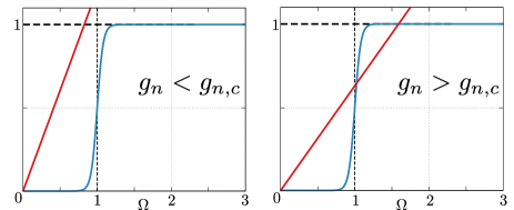
Figure 2: (Color online) Graphical analysis of Eq. (21) for $g_{n}<g_{n,c}$ (left) and $g_{n}>g_{n,c}$ (right) for a certain $n$ and fixed temperature. The red straight line corresponds to the first term, $\bigr{(}\frac{g_{n}}{g_{n,c}}\bigr{)}^{2}\Omega$, the other blue curved line corresponds to $q(\Omega)$ of Eq. (21) involving the hyperbolic functions. Of physical relevance is the region $\Omega>1$ only. Thus, for $g<g_{n,c}$ no physical solution is possible, whereas for $g_{n}>g_{n,c}$ a physical solution might exist.

On the other hand, for $g_{n}>g_{n,c}$, non-trivial solutions of Eq. (21) can exist. In the right panel of Fig. 2, both terms of Eq. (21) are drawn. We see that for every finite temperature, the two curves always intersect twice, so that Eq. (21) always has two solutions. Of course, for a differentiable $f$, the two solutions cannot both correspond to minima of $f$. Hence, one solution stems from a maximum and the other from a minimum. Since the right side of Eq. (21) is the derivative of $f$, its sign-change signals whether a maximum (plus-minus sign change) or a minimum (minus-plus sign change) is passed when $\Omega$ is increased. Therefore, the first solution corresponds to a maximum and the second to a minimum.

We gain additional insight, if we directly analyse $f(y_{n})$ for different coupling strengths [$f(y_{n})\equiv f(y_{1},0,0,0)$ from Eq. (9), w.l.o.g. $n=1$]. This is shown in Fig. 3. We see that for small coupling strengths, $f(y_{n})$ has one local minimum only which is located at $y_{n}=0$, the trivial solution. If the coupling strength is increased, a maximum-minimum pair forms at finite values of $y_{n}$. In general, this local minimum at $y_{n}>0$ is energetically higher than the local minimum of the trivial solution at $y_{n}=0$, cf. Fig. 3. Hence, the trivial solution still minimises $f(y_{n})$ globally. However, if the coupling strength is increased even further, the local minimum at $y_{n}>0$ becomes the global minimum. So we see that the position $y_{n,0}$ of the global minimum jumps at a certain value of the coupling strength from zero to a finite value.

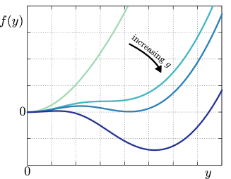
Figure 3: (Color online) The function $f$ of Eq. (9) with $z_{n}=0=y_{2}$, and $y_{1}=y$ for fixed temperature. The coupling strength $g$ increases from the upper to the lower curves. The units are arbitrary and $f$ has been rescaled for comparison, such that $f(0)=0$ for all coupling strengths $g$. On increasing $g$, a local minimum forms distant from the origin. For large $g$ this minimum eventually becomes a global minimum.

The above discussion refers to the case $\delta=0$. However, for finite $\delta$, the results are qualitatively the same. We discuss the properties of the phase transition for finite $\delta$ below.

III The Phase Transition

In the above analysis, we have shown the existence of three different minima of $f$ appearing in the exponent of the integrand of the partition sum. We have also shown that for a given temperature $T$, we find coupling strengths $g_{1,c}(T),g_{2,c}(T)$, below which the trivial solution $y_{1,0}=y_{2,0}=0$ minimises $f$. In Eq. (13), $y_{n,0}$ measures the macroscopic occupation of the bosonic modes and can therefore serve as an order parameter of the phase transition. Hence, in the parameter regime where the trivial solution minimises $f$, the system is in the normal phase.

In addition, above the coupling strengths $g_{1,c}(T),g_{2,c}(T)$, $f$ is minimised by non-zero values of either $y_{1,0}$ or $y_{2,0}$. The first corresponds to the red superradiant phase, the latter to the blue superradiant phase of Ref. Hayn et al. (2011). The two superradiant phases at non-zero temperatures show only one macroscopically occupied bosonic mode as well; mode one for the blue superradiant phase and mode two for the red superradiant phase, while the occupation of the other mode is zero.

As we have seen in the previous section, the location of the global minimum $y_{n,0}$ jumps from the trivial solution to non-zero solutions. A jump of the order parameter defines a first-order phase transition. Therefore, the finite-temperature superradiant phase transition in the Lambda-model is a first-order phase transition. Hence, the continuous phase transition at zero temperature of Ref. Hayn et al. (2011) transforms into a first order phase transition at finite temperatures.

So far, we have identified the phases and phase transitions using the occupation of the bosonic modes. In the following, we will further characterise the phases using observables of the three-level systems.

III.1 Normal Phase

In the normal phase with $y_{1,0}=y_{2,0}=0$, the Hamiltonian $\hat{h}_{0}$ is diagonal and the eigenvectors $\bm{w}_{k}$ are given by Cartesian unit vectors. Hence, the expectation value of all collective operators $\hat{A}_{n}^{\ m}$ with $n\neq m$ vanish. Conversely for the diagonal operators $\hat{A}_{n}^{\ n}$, the occupations; their expectation values are given by

$$\braket{\hat{A}_{1}^{\ 1}} =\mathcal{N}\,\frac{1}{1+\mathrm{e}^{-\beta\delta}+\mathrm{e}^{-\beta\Delta}},$$ (23)

$$\braket{\hat{A}_{2}^{\ 2}} =\mathcal{N}\,\frac{\mathrm{e}^{-\beta\delta}}{1+\mathrm{e}^{-\beta\delta}+\mathrm{e}^{-\beta\Delta}},$$ (24)

and

$$\braket{\hat{A}_{3}^{\ 3}} =\mathcal{N}\,\frac{\mathrm{e}^{-\beta\Delta}}{1+\mathrm{e}^{-\beta\delta}+\mathrm{e}^{-\beta\Delta}}.$$ (25)

Here, we explicitly see that in the normal phase the expectation values are independent of the coupling strengths $g_{1}$ and $g_{2}$. Furthermore we note that for finite temperatures, in addition to the single-particle ground state $\ket{1}$, the energetically higher lying single-particle states $\ket{2}$ and $\ket{3}$ are macroscopically excited as well. Hence in contrast to the bosonic modes, the particle part of the system gets thermally excited. From that point of view, i. e. concerning the populations of the single-particle energy levels, the particle system in the normal phase behaves like a normal thermodynamical system.

III.2 Superradiant Phases

For the superradiant phases, we cannot give explicit expressions for the expectation values, neither for finite or vanishing $\delta$. That is because we need to compute the minimum of $f$ numerically. Though for $\delta=0$, we can say that some expectation values are exactly zero. This will be done next, separately for the red and the blue superradiant phases.

Red Superradiant Phase

First consider the red superradiant phase with $y_{1,0}\equiv y_{0}\neq 0$ and $y_{2,0}=0$. Then, the single-particle Hamiltonian $\hat{h}(y_{0},0)$ reads [cf. Eq. (7)]

$$\hat{h}(y_{0},0)=\begin{pmatrix}0&0&2g_{1}y_{0}\\ 0&0&0\\ 2g_{1}y_{1}&0&\Delta\end{pmatrix},$$ (26)

and its exponential has the form

$$\mathrm{e}^{-\beta\hat{h}(y_{0},0)}=\begin{pmatrix}a_{+}&0&b_{1}\\ 0&1&0\\ b_{1}&0&a_{-}\end{pmatrix}.$$ (27)

The matrix elements $a_{\pm}$ and $b_{n}$ are given by (the matrix element $b_{2}$ is needed below).

$$a_{\pm} =\mathrm{e}^{-\frac{\beta\Delta}{2}}\left(\cosh\Bigl{[}\frac{\beta\Delta\Omega}{2}\Bigr{]}\pm\frac{\sinh\Bigl{[}\frac{\beta\Delta\Omega}{2}\Bigr{]}}{\Omega}\right),$$ (28)

$$b_{n} =-\frac{4g_{n}y_{n}}{\Delta\Omega}\mathrm{e}^{-\frac{\beta\Delta}{2}}\,\sinh\Bigl{[}\frac{\beta\Delta\Omega}{2}\Bigr{]},\quad n=(1,2).$$ (29)

The product of the exponential operator, Eq. (27), with matrices of the form

$$\begin{pmatrix}0&M_{12}&0\\ M_{21}&0&M_{23}\\ 0&M_{32}&0\end{pmatrix}$$ (30)

is traceless. Therefore, the expectation values of the collective operators $\hat{A}_{1}^{\ 2}$, $\hat{A}_{2}^{\ 3}$ and their Hermitian conjugates are zero, i. e. there is no spontaneous polarisation between both the single-particle states $\ket{1}$ and $\ket{2}$, and the single-particle states $\ket{2}$ and $\ket{3}$. Contrary, the polarisation in the left branch of the Lambda-model, i. e. between the states $\ket{1}$ and $\ket{3}$, is finite and macroscopic.

Blue Superradiant Phase

For the blue superradiant case, the discussion is similar. Here we have $y_{2,0}\equiv y_{0}\neq 0$ and $y_{1,0}=0$, and the exponential of the single-particle Hamiltonian reads

$$\mathrm{e}^{-\beta\hat{h}(0,y_{0})}=\begin{pmatrix}1&0&0\\ 0&a_{+}&b_{2}\\ 0&b_{2}&a_{-}\end{pmatrix}.$$ (31)

The matrix elements are given above, Eqs (28), (29). Now, the product of the exponential operator, Eq. (31), with matrices of the form

$$\begin{pmatrix}0&M_{12}&M_{13}\\ M_{21}&0&0\\ M_{31}&0&0\end{pmatrix}$$ (32)

is traceless and thus expectation values of the collective operators $\hat{A}_{1}^{\ 2}$, $\hat{A}_{1}^{\ 3}$ and their Hermitian conjugates are zero. On the other hand, the expectation value of the operators $\hat{A}_{2}^{\ 3}$, $\hat{A}_{3}^{\ 2}$ is finite and macroscopic. Hence, only the transition in the right branch of the Lambda-model is spontaneously polarised.

In conclusion, we find that in the superradiant phases at finite temperature, only the corresponding branch of the Lambda-model shows spontaneous polarisation; the left branch in the red superradiant phase and the right branch in the blue superradiant phase. In the normal phase, the polarisation is completely absent. Hence, in contrast to the populations of the atomic system, the polarisations are not thermally excited and show a genuine quantum character. Thus, both the polarisations and the occupations of the two resonator modes show a similar behaviour in the three phases. Therefore we have two sets of observables, the polarisations for the three-level systems and the occupations of the bosonic modes, to detect the superradiant phase transition at finite temperatures.

III.3 Numerical evaluation of the Partition Sum

The above analysis for vanishing $\delta$ already shows that the phase transition in the Lambda-model for finite temperatures is a first-order phase transition. This fact renders the calculation of the exact location of the phase transition with our methods impossible. This can be understood with the help of the free energy as follows. In the thermodynamic limit, the global minimum of the free energy defines the thermodynamic phase of the system. We explicitly saw this when we have computed the partition sum. In a phase transition, the system changes from one thermodynamic state to another thermodynamic state. This new state corresponds to a different, now global minimum of the free energy.

For continuous phase transitions, the new minimum evolves continuously from the first minimum and the first minimum changes its character to a maximum. Hence, the continuous phase transition is characterised by a sign-change of the curvature of the free energy at the position of the minimum of the state describing the normal phase. Often, this is tractable analytically.

In contrast in the case of first-order phase transitions, the new global minimum of the free energy appears distant from the old global minimum of the free energy, cf. Fig. 3. There are still two minima and we cannot detect the phase transition by the curvature of the free energy. Thus to find the phase transition for first-order phase transitions, we first need to find all minima of the free energy and then find the global minima of these. This has to be done numerically here.

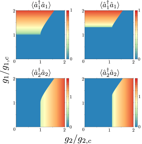
Figure 4: (Color online) Numerical computation of the scaled occupations $\braket{\hat{a}_{n}^{\dagger}\hat{a}_{n}}/\mathcal{N}$ of the two bosonic modes for $k_{\mathrm{B}}T=0.001\,\Delta$ (left) and $k_{\mathrm{B}}T=0.25\,\Delta$ (right). The parameters are set to $\Delta=1$, $\delta=0.1$, $\omega_{1}=1.1$, and $\omega_{2}=0.8$. The computation has been done in the thermodynamic limit using Laplace’s method.

For the numerical computation, we do not solve Eq. (18), but we test for the minima of $f(y_{1},y_{2})$, Eq. (9), directly. Therefore, we apply a brute-force method, i. e. we look for the smallest value of $f(y_{1},y_{2})$ on a $y_{1}$–$y_{2}$ grid. Due to the reflection symmetry of $f(y_{1},y_{2})$, we can confine the grid to positive values for $y_{1}$ and $y_{2}$. This yields the position of the minimum $(y_{1,0},y_{2,0})$. Then we compute the eigenvalues and eigenvectors of the Hamiltonian $\hat{h}$, at this point and obtain via Eq. (39) the expectation values for the operators of the bosonic modes, and via Eq. (17) the corresponding expectation values for the three-level systems.

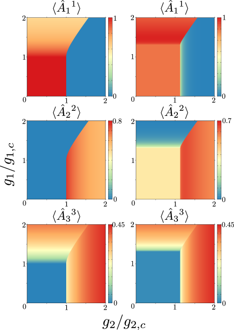
Figure 5: (Color online) Numerical computation of the scaled occupations $\braket{\hat{A}_{n}^{\ n}}\mathcal{N}$ of the single-particle energy levels of the three-level systems for $k_{\mathrm{B}}T=0.001\,\Delta$ (left) and $k_{\mathrm{B}}T=0.25\,\Delta$ (right). Parameters as in Fig. 4.

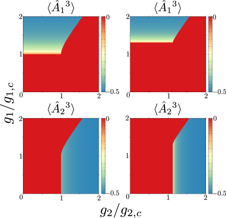
Figure 6: (Color online) Numerical computation of the scaled polarisations $\braket{\hat{A}_{1}^{\ 3}}/\mathcal{N}$, $\braket{\hat{A}_{2}^{\ 3}}/\mathcal{N}$ of the three-level systems for $k_{\mathrm{B}}T=0.001\,\Delta$ (left) and $k_{\mathrm{B}}T=0.25\,\Delta$ (right). Parameters as in Fig. 4.

Fig. 4, 5, 6 show the occupation $\braket{\hat{a}^{\dagger}_{n}\hat{a}_{n}}$ of the modes of the resonator, the occupation $\hat{A}_{n}^{\ n}$ of the single-particle levels of the atoms, and the polarisations $\hat{A}_{1}^{\ 3}$, $\hat{A}_{2}^{\ 3}$ of the atoms for low and high temperatures, respectively. All plots have been generated numerically for finite values of $\delta$.

These figures corroborate our findings from the analytical discussion of the partition sum for vanishing $\delta$. We see three phases: a normal phase for coupling strengths $g_{1}$ and $g_{2}$ below the critical coupling strengths $g_{1,c}$ and $g_{2,c}$, a red superradiant phase for large coupling strengths $g_{1}$ above the critical coupling strength $g_{1,c}$, and a blue superradiant phase for coupling strengths $g_{2}$ above the critical coupling strength $g_{2,c}$.

The normal phase is characterised by a zero occupation of both bosonic modes (Fig. 4) In addition, the polarisation, or coherence, of the three-level systems is zero in the normal phase (Fig. 6).

In contrast, to the normal phase, the two superradiant phases are characterised by a macroscopic occupation of only one of the two bosonic modes; mode one in the red superradiant phase and mode two in the blue superradiant phase. In addition, the red (blue) superradiant phase shows a spontaneous polarisation $\braket{\hat{A}_{1}^{\ 3}}$ ($\braket{\hat{A}_{2}^{\ 3}}$).

We see that these defining properties remain for increasing temperature (right part of Figs. 4-6). As discussed in Sec. III.1, we see that the population $\braket{\hat{A}_{2}^{\ 2}}$ of the single-particle energy level $\ket{2}$ increases for rising temperature. The same is true for the occupation $\braket{\hat{A}_{3}^{\ 3}}$, though this is not visible in the right part of Fig. 5 due to the fact that the temperature is yet too small.

From the Figs. 4-6 we also see that the shape of the phase boundary remains a straight line between the normal and the two superradiant phases. Between the red and the blue superradiant phases, the form of the phase boundary seems to persist as well. The only effect of the rising temperature is a shift of the phase boundary towards higher values of the coupling strengths $g_{1}$ and $g_{2}$. This is visualised in Fig. 7 where the polarisation $\braket{\hat{A}_{1}^{\ 3}}$ of the transition $\ket{1}\leftrightarrow\ket{3}$ of the three-level systems is shown for variable coupling strength $g_{1}$ and temperature $T$. The coupling strength of the second mode is fixed to $g_{2}=0.2\,g_{2,c}$. We see that for increasing temperature, the superradiant phase diminishes.

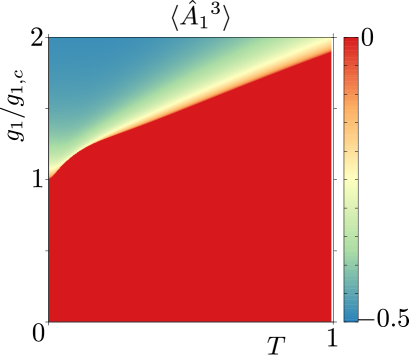
Figure 7: (Color online) Numerical computation of the scaled polarisation $\braket{\hat{A}_{1}^{\ 3}}/\mathcal{N}$ of the transition $\ket{1}\leftrightarrow\ket{3}$ of the three-level system. Parameters as in Fig. 4 and $g_{2}=0.2\,g_{2,c}$.

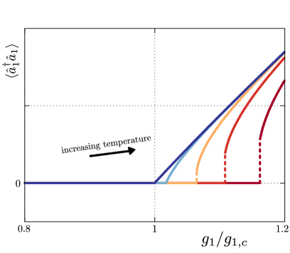
Figure 8: (Color online) Occupations $\braket{\hat{a}_{1}^{\dagger}\hat{a}_{1}}$ of the first bosonic mode as a function of the coupling strength $g_{1}$ for fixed coupling strength $g_{2}=0.2g_{2,c}$ and rising temperature (left to right, blue to red, respectively). The other parameters are set to $\Delta=1$, $\delta=0.1$, $\omega_{1}=1.1$, and $\omega_{2}=0.8$.

In addition to the shift of the phase boundary, the jump in the observables at this first-order phase transition increases. This is shown in Fig. 8 for the occupation $\braket{\hat{a}_{1}^{\dagger}\hat{a}_{1}}$ of the first bosonic mode. Of course, numerically, jumps are hard to detect since we get a discrete set of points as an output anyway. However, the dotted lines in Fig. 8 connect two largely separated points; each of the lines consists of 1000 data points. Thus we can really speak of jumps in the observables and thus of a first-order phase transition.

III.4 Zero-Temperature Limit

Lastly, we analyse the zero-temperature limit of the Lambda-model for $\delta=0$. For decreasing temperature, the function $q(\Omega)$, Eq. (19), becomes more and more step function like. Indeed, for $\beta\Delta\gg 1$, $q(\Omega)$ can be written as a Fermi function, and eventually in the limit $\beta\Delta\rightarrow\infty$, $q(\Omega)$ is given by

$$q(\Omega)=\begin{cases}0&,\quad\Omega<1\\ 1&,\quad\Omega>1.\end{cases}$$ (33)

Hence at zero temperature, Eq. (21) has always a unique solution for coupling strengths $g_{n}>g_{n,c}$. In addition, since $f(y)$ shows no additional maximum, we have a continuous phase transition in this quantum limit.

Furthermore, we can also compute the position of the minimum of $f$. In the limit $T\rightarrow 0$, Eq. (21) reads

$$0=\Bigl{(}\frac{g_{n,c}}{g_{n}}\Bigr{)}^{2}\sqrt{1+\frac{4\hbar\omega_{n}}{\Delta}\Bigl{(}\frac{g_{n}}{g_{n,c}}\Bigr{)}^{2}y_{n}^{2}\;}-1.$$ (34)

Solving for $y_{n}$, we obtain

$$y_{n}=\pm\frac{g}{\hbar\omega_{n}}\sqrt{1-\Bigl{(}\frac{g_{n,c}}{g_{n}}\Bigr{)}^{4}\,}.$$ (35)

If we identify $y_{n}$ with the mean-fields $\varphi_{n}$ of Ref. Hayn et al. (2011), we reproduce our results Hayn et al. (2011) for the superradiant phases of the quantum phase transition of the Lambda-model.

The mean-fields $\Psi_{n}$ of Ref. Hayn et al. (2011) can be reproduced as well. Consider for instance $\Psi_{3}$ which is related to $\braket{\hat{A}_{3}^{\ 3}}$ through $\braket{\hat{A}_{3}^{\ 3}}=\mathcal{N}\Psi_{3}^{2}$, except for a possible phase. Using the results for the Boltzmann operator in the red superradiant phase, Eq. (31), plus the above expression for $y_{1}$, Eq. (35), and finally insert everything into the expectation value of Eq. (16), we obtain

$$\braket{\hat{A}_{3}^{\ 3}}=\frac{\mathcal{N}}{2}\frac{1-\mathrm{e}^{\beta\Delta\Omega}+\Bigl{(}1+\mathrm{e}^{\beta\Delta\Omega}\Bigr{)}\Omega}{\bigl{[}1+\mathrm{e}^{\beta\Delta\Omega}+\mathrm{e}^{\frac{\beta\Delta}{2}(\Omega+1)}\bigr{]}\Omega},$$ (36)

which in the zero-temperature limit $\beta\Delta\rightarrow\infty$ reduces to

$$\braket{\hat{A}_{3}^{\ 3}}=\frac{\mathcal{N}}{2}\frac{\Omega-1}{\Omega}.$$ (37)

Here, $\Omega=\Omega(y_{1})$ from Eq. (22). If we finally insert the position $y_{1}$ of the minimum of the free energy, Eq. (35), the population of the third single-particle energy level in the zero-temperature limit is given by

$$\braket{\hat{A}_{3}^{\ 3}}=\frac{\mathcal{N}}{2}\Bigl{[}1-\Bigl{(}\frac{g_{1,c}}{g_{1}}\Bigr{)}^{2}\Bigr{]}$$ (38)

which agrees with the findings of Ref. Hayn et al. (2011) for $\Psi_{3}$. Applying the same technique, we can obtain the expectation values of all other collective atomic operators $\hat{A}_{n}^{\ m}$ in both superradiant phases. This again coincides with the results of Ref. Hayn et al. (2011).

IV Conclusion

We have analysed the Lambda-model in the thermodynamic limit at finite temperatures using the partition sum of the Hamiltonian. Compared to the quantum phase transition of this model Hayn et al. (2011), we found that at finite temperatures the properties of the phases and phase transition partially persist. Namely, we found three phases: a normal and two superradiant phases. These have the same properties as in the quantum limit. For small couplings and/or at high temperatures, the system is in the normal phase where all particles are in their respective single-particle ground-state and both bosonic modes are in their vacuum state. If one of the coupling strengths is increased above a temperature-dependent critical coupling strength, the system undergoes a phase transition into a superradiant phase wich is characterised by a macroscopic occupation of one of the bosonic modes only and a spontaneaous polarisation of the corresponding branch of the three-level system.

A new characteristic of the phase transition at finite temperatures is the appearance of first-order phase transitions only. For the quantum phase transition we already found first-order phase transitions between the normal and the red superradiant phase and between the two superradiant phases. Here, at finite temperatures, the phase transition from the normal to the blue superradiant phase becomes a first-order phase transition as well. This change of the order of the phase transition would appear for a single bosonic mode as well. Hence, it is due to the additional single-particle energy level that first-order phase transitions show up. In addition, we emphasise that even in the degenerate limit, $\delta\rightarrow 0$, the phase transitions from the normal to both superradiant phases are of first order.

It is remarkable that in contrast to the original Dicke model, the mean-field phase transitions at finite temperatures are not continuous. This facet becomes significant if real atoms and photons are considered. Here, for the original Dicke model with its continuous phase transition, there exists a no-go theorem Rzażewski et al. (1975, 1976); Rzażewski and Wódkiewicz (1976); Knight et al. (1978); Bialynicki-Birula and Rza¸żewski (1979); Slyusarev and Yankelevich (1979); Nataf and Ciuti (2010a); Viehmann et al. (2011). However for first-order mean-field quantum phase transitions, it is known Hayn et al. (2012); Baksic et al. (2013) that this no-go theorem does not apply and superradiant phase transitions occur. We expect an identical conclusion for the Lambda-model at finite temperatures.

V Acknowledgements

This work was supported by the Deutsche Forschungsgemeinschaft within the SFB 910, the GRK 1558, and the projects BR 1528/82 and 1528/9.

VI Appendix

VI.1 Expectation Values of Bosonic Mode Operators

We calculate the expectation value of functions $G$ of operators of the two bosonic modes as,

$$\braket{G(\hat{a}^{\dagger}_{1},\hat{a}_{1},\hat{a}^{\dagger}_{2},\hat{a}_{2})}=\frac{1}{\mathcal{Z}}\mathrm{Tr}\{G(\hat{a}^{\dagger}_{1},\hat{a}_{1},\hat{a}^{\dagger}_{2},\hat{a}_{2})\mathrm{e}^{-\beta\hat{H}}\}$$ (39)

$$=\frac{1}{\mathcal{Z}}\int_{\mathbb{C}^{2}}\frac{\mathrm{d}^{2}\alpha_{1}\mathrm{d}^{2}\alpha_{2}}{\pi^{2}}G(\alpha_{1}^{*},\alpha_{1},\alpha_{2}^{*},\alpha_{2})$$ (40)

$$\qquad\times\mathrm{e}^{-\beta\sum_{n=1}^{2}\hbar\omega_{n}\lvert\alpha_{n}\rvert^{2}}\mathrm{Tr}\{\mathrm{e}^{-\beta\hat{h}}\}^{\mathcal{N}}$$ (41)

$$=\frac{1}{\mathcal{Z}}\frac{\mathcal{N}^{2}}{\pi^{2}}\int_{\mathbb{R}^{2}}\mathrm{d}y_{1}\mathrm{d}y_{2}G(\sqrt{\mathcal{N}}y_{1},\sqrt{\mathcal{N}}y_{1},\sqrt{\mathcal{N}}y_{2},\sqrt{\mathcal{N}}y_{2})$$ (42)

$$\qquad\times\mathrm{e}^{-\beta f}$$ (43)

$$=G(\sqrt{\mathcal{N}\,}y_{1,0},\sqrt{\mathcal{N}\,}y_{1,0},\sqrt{\mathcal{N}\,}y_{2,0},\sqrt{\mathcal{N}\,}y_{2,0}).$$ (44)

In the last step we used that the exponential dominates for large $\mathcal{N}$. Hence, the function $G$ can be considered constant and the remaining integral plus the prefactor is equal to the partition sum.

VI.2 Expectation Values of Operators of the Three-Level Systems

For mean values of collective operators $\hat{M}$ (cf. II.3) of the three-level systems we have,

$$\braket{\hat{M}} =\frac{1}{\mathcal{Z}}\mathrm{Tr}\{\hat{M}\mathrm{e}^{-\beta\hat{H}}\}$$ (45)

$$=\frac{1}{\mathcal{Z}}\int_{\mathbb{C}^{2}}\frac{\mathrm{d}^{2}\alpha_{1}\mathrm{d}^{2}\alpha_{2}}{\pi^{2}}\mathrm{e}^{-\beta\sum_{n=1}^{2}\hbar\omega_{n}\lvert\alpha_{n}\rvert^{2}}$$ (46)

$$\qquad\times\sum_{k=1}^{\mathcal{N}}\mathrm{Tr}\Bigl{\{}\hat{m}^{(k)}\mathrm{e}^{-\beta\hat{h}^{(1)}}\cdot\ldots\cdot\mathrm{e}^{-\beta\hat{h}^{(\mathcal{N})}}\Bigr{\}}$$ (47)

$$=\frac{1}{\mathcal{Z}}\int_{\mathbb{C}^{2}}\frac{\mathrm{d}^{2}\alpha_{1}\mathrm{d}^{2}\alpha_{2}}{\pi^{2}}\mathrm{e}^{-\beta\sum_{n=1}^{2}\hbar\omega_{n}\lvert\alpha_{n}\rvert^{2}}$$ (48)

$$\qquad\times\mathrm{Tr}\{\mathrm{e}^{-\beta\hat{h}}\}^{\mathcal{N}}\mathcal{N}\frac{\mathrm{Tr}\Bigl{\{}\hat{m}\mathrm{e}^{-\beta\hat{h}}\Bigr{\}}}{\mathrm{Tr}\{\mathrm{e}^{-\beta\hat{h}}\}}$$ (49)

$$=\mathcal{N}\frac{\mathrm{Tr}\Bigl{\{}\hat{m}\,\mathrm{e}^{-\beta\hat{h}_{0}}\Bigr{\}}}{\mathrm{Tr}\{\mathrm{e}^{-\beta\hat{h}_{0}}\}}$$ (50)

$$\equiv\mathcal{N}\braket{\hat{m}}_{0},$$ (51)

with $\hat{h}_{0}=\hat{h}(y_{1,0},y_{2,0})$.

References

- Dicke (1954) R. H. Dicke, Phys. Rev. 93, 99 (1954).
- Hepp and Lieb (1973a) K. Hepp and E. H. Lieb, Ann. Phys. 76, 360 (1973a).
- Baumann et al. (2010) K. Baumann, C. Guerlin, F. Brennecke, and T. Esslinger, Nature (London) 464, 1301 (2010).
- Baumann et al. (2011) K. Baumann, R. Mottl, F. Brennecke, and T. Esslinger, Phys. Rev. Lett. 107, 140402 (2011).
- Ritsch et al. (2013) H. Ritsch, P. Domokos, F. Brennecke, and T. Esslinger, Rev. Mod. Phys. 85, 553 (2013).
- Hamner et al. (2014) C. Hamner, C. Qu, Y. Zhang, J. Chang, M. Gong, C. Zhang, and P. Engels, Nature Communications 5, 4023 (2014).
- Klinder et al. (2015) J. Klinder, H. Keßler, M. R. Bakhtiari, M. Thorwart, and A. Hemmerich, Phys. Rev. Lett. 115, 230403 (2015).
- Dimer et al. (2007) F. Dimer, B. Estienne, A. S. Parkins, and H. J. Carmichael, Phys. Rev. A 75, 013804 (2007).
- Baden et al. (2014) M. P. Baden, K. J. Arnold, A. L. Grimsmo, S. Parkins, and M. D. Barrett, Phys. Rev. Lett. 113, 020408 (2014).
- Keeling et al. (2010) J. Keeling, M. J. Bhaseen, and B. D. Simons, Phys. Rev. Lett. 105, 043001 (2010).
- Nagy et al. (2011) D. Nagy, G. Szirmai, and P. Domokos, Phys. Rev. A 84, 043637 (2011).
- Öztop et al. (2012) B. Öztop, M. Bordyuh, O. E. Müstecaplioglu, and H. E. Türeci, New Journal of Physics 14, 085011 (2012).
- Bhaseen et al. (2012) M. J. Bhaseen, J. Mayoh, B. D. Simons, and J. Keeling, Phys. Rev. A 85, 013817 (2012).
- Kónya et al. (2012) G. Kónya, D. Nagy, G. Szirmai, and P. Domokos, Phys. Rev. A 86, 013641 (2012).
- Torre et al. (2013) E. G. D. Torre, S. Diehl, M. D. Lukin, S. Sachdev, and P. Strack, Phys. Rev. A 87, 023831 (2013).
- Kopylov et al. (2013) W. Kopylov, C. Emary, and T. Brandes, Phys. Rev. A 87, 043840 (2013).
- Genway et al. (2014) S. Genway, W. Li, C. Ates, B. P. Lanyon, and I. Lesanovsky, Phys. Rev. Lett. 112, 023603 (2014).
- Dalla Torre et al. (2016) E. G. Dalla Torre, Y. Shchadilova, E. Y. Wilner, M. D. Lukin, and E. Demler (2016), eprint arXiv:1608.06293.
- Gelhausen et al. (2016) J. Gelhausen, M. Buchhold, and P. Strack (2016), eprint arXiv:1605.07637.
- Konya et al. (2011) G. Konya, G. Szirmai, and P. Domokos, The European Physical Journal D 65, 33 (2011).
- Piazza et al. (2013) F. Piazza, P. Strack, and W. Zwerger, Annals of Physics 339, 135 (2013).
- Strack and Sachdev (2011) P. Strack and S. Sachdev, Phys. Rev. Lett. 107, 277202 (2011).
- Inoue (2012) J.-i. Inoue, Journal of Physics A: Mathematical and Theoretical 45, 305003 (2012).
- Goto and Ichimura (2008) H. Goto and K. Ichimura, Phys. Rev. A 77, 053811 (2008).
- Tsyplyatyev and Loss (2009) O. Tsyplyatyev and D. Loss, Phys. Rev. A 80, 023803 (2009).
- Vidal and Dusuel (2006) J. Vidal and S. Dusuel, Europhys. Lett. 74, 817 (2006).
- Liberti et al. (2006) G. Liberti, F. Plastina, and F. Piperno, Phys. Rev. A 74, 022324 (2006).
- Bakemeier et al. (2012) L. Bakemeier, A. Alvermann, and H. Fehske, Phys. Rev. A 85, 043821 (2012).
- Bastidas et al. (2012) V. M. Bastidas, C. Emary, B. Regler, and T. Brandes, Phys. Rev. Lett. 108, 043003 (2012).
- Francica et al. (2016) G. Francica, S. Montangero, M. Paternostro, and F. Plastina (2016), eprint arXiv:1608.05049.
- Brandes (2013) T. Brandes, Phys. Rev. E 88, 032133 (2013).
- Yi-Xiang et al. (2013) Y. Yi-Xiang, J. Ye, and W.-M. Liu, Scientific Reports 3, 3476 (2013).
- Baksic and Ciuti (2014) A. Baksic and C. Ciuti, Phys. Rev. Lett. 112, 173601 (2014).
- Grimsmo et al. (2014) A. L. Grimsmo, A. S. Parkins, and B.-S. Skagerstam, New Journal of Physics 16, 065004 (2014).
- Kopylov et al. (2015) W. Kopylov, C. Emary, E. Schöll, and T. Brandes, New Journal of Physics 17, 013040 (2015).
- Nataf and Ciuti (2010a) P. Nataf and C. Ciuti, Nat. Commun. 1, 72 (2010a).
- Nataf and Ciuti (2010b) P. Nataf and C. Ciuti, Phys. Rev. Lett. 104, 023601 (2010b).
- Emary and Brandes (2003a) C. Emary and T. Brandes, Phys. Rev. E 67, 066203 (2003a).
- Emary and Brandes (2003b) C. Emary and T. Brandes, Phys. Rev. Lett. 90, 044101 (2003b).
- Wang and Hioe (1973) Y. K. Wang and F. T. Hioe, Phys. Rev. A 7, 831 (1973).
- Hepp and Lieb (1973b) K. Hepp and E. H. Lieb, Phys. Rev. A 8, 2517 (1973b).
- Carmichael et al. (1973) H. J. Carmichael, C. W. Gardiner, and D. F. Walls, Physics Letters A 46, 47 (1973).
- Brandes (2005) T. Brandes, Phys. Rep. 408, 315 (2005).
- Paraan and Silva (2009) F. N. C. Paraan and A. Silva, Phys. Rev. E 80, 061130 (2009).
- Fusco et al. (2016) L. Fusco, M. Paternostro, and G. De Chiara (2016), eprint arXiv:1605.06286.
- Pérez-Fernández et al. (2011a) P. Pérez-Fernández, P. Cejnar, J. M. Arias, J. Dukelsky, J. E. García-Ramos, and A. Relaño, Phys. Rev. A 83, 033802 (2011a).
- Pérez-Fernández et al. (2011b) P. Pérez-Fernández, A. Relaño, J. M. Arias, P. Cejnar, J. Dukelsky, and J. E. García-Ramos, Phys. Rev. E 83, 046208 (2011b).
- Puebla et al. (2013) R. Puebla, A. Relaño, and J. Retamosa, Phys. Rev. A 87, 023819 (2013).
- Puebla and Relaño (2013) R. Puebla and A. Relaño, EPL 104, 50007 (2013).
- Bastarrachea-Magnani et al. (2014) M. A. Bastarrachea-Magnani, S. Lerma-Hernández, and J. G. Hirsch, Phys. Rev. A 89, 032101 (2014).
- Bastarrachea-Magnani et al. (2015) M. A. Bastarrachea-Magnani, B. López-del Carpio, S. Lerma-Hernández, and J. G. Hirsch, Physica Scripta 90, 068015 (2015).
- Lóbez and Relaño (2016) C. M. Lóbez and A. Relaño, Phys. Rev. E 94, 012140 (2016).
- Bastarrachea-Magnani et al. (2016) M. A. Bastarrachea-Magnani, S. Lerma-Hernández, and J. G. Hirsch (2016), eprint arXiv:1605.05357.
- Kloc et al. (2016) M. Kloc, P. Stransky, and P. Cejnar (2016), eprint arXiv:1609.02758.
- Hayn et al. (2011) M. Hayn, C. Emary, and T. Brandes, Phys. Rev. A 84, 053856 (2011).
- Hayn et al. (2012) M. Hayn, C. Emary, and T. Brandes, Phys. Rev. A 86, 063822 (2012).
- Rzażewski et al. (1975) K. Rzażewski, K. Wódkiewicz, and W. Żakowicz, Phys. Rev. Lett. 35, 432 (1975).
- Rzażewski et al. (1976) K. Rzażewski, K. Wódkiewicz, and W. Żakowicz, Physics Letters A 58, 211 (1976).
- Rzażewski and Wódkiewicz (1976) K. Rzażewski and K. Wódkiewicz, Phys. Rev. A 13, 1967 (1976).
- Knight et al. (1978) J. M. Knight, Y. Aharonov, and G. T. C. Hsieh, Phys. Rev. A 17, 1454 (1978).
- Bialynicki-Birula and Rza¸żewski (1979) I. Bialynicki-Birula and K. Rza¸żewski, Phys. Rev. A 19, 301 (1979).
- Slyusarev and Yankelevich (1979) V. A. Slyusarev and R. P. Yankelevich, Theoretical and Mathematical Physics 40, 641 (1979).
- Viehmann et al. (2011) O. Viehmann, J. von Delft, and F. Marquardt, Phys. Rev. Lett. 107, 113602 (2011).
- Ciuti and Nataf (2012) C. Ciuti and P. Nataf, Phys. Rev. Lett. 109, 179301 (2012).
- Viehmann et al. (2012) O. Viehmann, J. von Delft, and F. Marquardt (2012), eprint arXiv:1202.2916.
- Baksic et al. (2013) A. Baksic, P. Nataf, and C. Ciuti, Phys. Rev. A 87, 023813 (2013).
- Feynman (1972) R. P. Feynman, Statistical Mechanics — A Set of Lectures, Frontiers in Physics (W. A. Benjamin, Inc., Reading, Massachusetts, 1972), ISBN 0-805-32509-3.
- Glauber (1963) R. J. Glauber, Phys. Rev. 131, 2766 (1963).
- Arecchi et al. (1972) F. T. Arecchi, E. Courtens, R. Gilmore, and H. Thomas, Phys. Rev. A 6, 2211 (1972).
- Bender and Orszag (1999) C. M. Bender and S. A. Orszag, Advanced Mathematical Methods for Scientists and Engineers (Springer, New York [u.a.], 1999), ISBN 0-387-98931-5.