Abstract

We study the quantum correlations between the two remote qubits (sender and receiver) connected by the transmission line (homogeneous spin-1/2 chain) depending on the parameters of the sender’s and receiver’s initial states (control parameters). We consider two different measures of quantum correlations: the entanglement (a traditional measure) and the informational correlation (based on the parameter exchange between the sender and receiver). We find the domain in the control parameter space yielding (i) zero entanglement between the sender and receiver during the whole evolution period and (ii) non-vanishing informational correlation between the sender and receiver, thus showing that the informational correlation is responsible for the remote state creation. Among the control parameters, there are the strong parameters (which strongly effect the values of studied measures) and the weak ones (whose effect is negligible), therewith the eigenvalues of the initial state are given a privileged role. We also show that the problem of small entanglement (concurrence) in quantum information processing is similar (in certain sense) to the problem of small determinants in linear algebra. A particular model of 40-node spin-1/2 communication line is presented.

I Introduction

The formation and evolution of quantum correlations is one of the central problems of quantum information. Although quantum correlations are necessary to provide advantages of quantum information devices in comparison with their classical counterparts, the appropriate measure of these correlations is not well-established yet. For a long time, quantum entanglement HW ; Wootters was considered as a suitable measure, but recently quantum non-locality BDFMRSSW ; HHHOSS ; NC and speedup Meyer ; DSC ; DFC ; DV ; LBAW were observed in systems with minor entanglement. Therefore, the quantum discord was introduces as an alternative measure Z0 ; HV ; OZ ; Z . Still it is not clear whether the above mentioned quantum entanglement (even if its value is minor) captures all those quantum correlations that provide the advantages of any quantum device, or other types of correlations (which are captured, for instance, by discord rather then by entanglement) become more important in certain cases.

We may assume that the quantum correlations can be classified (with possible overlaps among different classes) so that a given quantum process is governed by a certain class of quantum correlations rather then by all of them. In this paper we are aimed on revealing those quantum correlations that are responsible for remote state creation ZZHE ; BPMEWZ ; BBMHP ; PBGWK2 ; PBGWK ; DLMRKBPVZBW ; XLYG ; LH , which is the further development of the problem of end-to-end quantum state transfer along a spin chain Bose ; CDEL ; ACDE ; KS ; GKMT ; WLKGGB ; NJ ; SAOZ ; CS ; BOWB ; ABCVV .

We consider a model of two remote one-qubit subsystems (called the sender ($S$) and the receiver ($R$)) connected to each other through the homogeneous spin-1/2 chain (called the transmission line ($TL$)). The initial state of the whole system is separated one with the both sender and receiver are in mixed states. Therefore, there is no quantum correlations between the sender and receiver initially. After the initial state is installed, the state of the whole system evolves under some Hamiltonian giving rise to mutual quantum correlations between the sender and receiver.

Our study is based on the comparative analysis of two classes of quantum correlations. The first class is captured by the sender-receiver entanglement (SR-entanglement), while the second class is captured by the so-called informational correlation which has been recently introduced Z_inf0 ; Z_inf . The latter quantity counts the number of parameters of the local unitary transformation initially applied to the sender (which are called eigenvector control-parameters below) that can be detected at the receiver. Informational correlation is discrete by its definition and it is directly related to the associated system of linear algebraic equations whose solvability turns into the appropriate determinant condition Z_inf .

We study the dependence of both the SR-entanglement and informational correlation on the parameters of the sender’s and receiver’s initial state which we call the control parameters naturally separated into eigenvalue and eigenvector parameters. In turn, we separate the eigenvector control-parameters into the strong control parameters (whose values strongly effect the quantum correlations) and weak control parameters (whose effect is negligible).

In addition, our study shows that there is a domain in the control parameters space which yields zero SR-entanglement during, at least, the considered evolution period. However, the parameters from this domain can also be transfered from the sender to the receiver (or vise-versa); therefore the informational correlation is non-zero and remote state creation is possible. Thus, the informational correlation serves as a measure selecting the quantum correlations responsible for the state transfer/creation, while the SR-entanglement doesn’t capture the required correlations.

At last, we show that the states with small SR-entanglement have the same pre-image in the control-parameter space as the states with small determinants. Therefore, the case of small determinants is likely to be the case when the advantage of quantumness disappears. In addition, this situation has something in common with so called fluctuations of entanglement FY ; Y showing that the value of these fluctuations can reach the value of entanglement itself, so that the calculated value of entanglement is not reliable in that case.

The paper is organized as follows. In Sec.II, we discuss the initial state of the communication line and classify the control parameters associated with this state. The SR-entanglement (SR-concurrence) and informational correlation as two different measures of quantum correlations are discussed in Sec.III. A particular model of quantum communication line based on the nearest-neighbor XY Hamiltonian is considered in Sec.IV. Both sender and receiver are one-qubit subsystems in our case. The brief comparative analysis of SR-concurrence and informational correlation is represented in Sec.V. Finally, the basic results are discussed in Sec.VI. Some additional details concerning the permanent characteristics of communication line, explicit form of the receiver’s density matrix, properties of determinants, the time instant for state registration are given in Appendix, Sec.VII.

II Classification of control parameters

II.1 Initial state

We consider a homogeneous spin-1/2 chain whose evolution is governed by some Hamiltonian commuting with the $z$-projection of the total spin momentum (the external magnetic field is $z$-directed). The whole $N$-spin communication line consists of three interacting subsystems: the one-qubit sender $S$ (the first qubit of the chain), the one-qubit receiver $R$ (the last qubit of the chain) and the transmission line $TL$ (a spin-chain connecting the sender and receiver). For the sake of simplicity, we consider the tensor-product initial state

$$\rho_{0}=\rho^{S}_{0}\otimes\rho^{TL}_{0}\otimes\rho^{R}_{0},$$ (1)

where $\rho^{S}_{0}$, $\rho^{TL}_{0}$ and $\rho^{S}_{0}$ are, respectively, the initial density matrices of the sender, transmission line and receiver, therewith $\rho^{TL}_{0}$ is the density matrix of the ground state,

$$\rho^{TL}={\mbox{diag}}(1,0,0,\dots),$$ (2)

and

$$\rho^{S}_{0}=U^{S}\Lambda^{S}(U^{S})^{+},\;\;\rho^{R}_{0}=U^{R}\Lambda^{R}(U^{R})^{+}.$$ (3)

Here the eigenvalue and eigenvector matrices read, respectively,

$$\Lambda^{S}={\mbox{diag}}(\lambda^{S},1-\lambda^{S}),\;\;\;\Lambda^{R}={\mbox{diag}}(\lambda^{R},1-\lambda^{R}),$$ (4)

and

$$U^{S}=\left(\begin{array}[]{cc}\cos\frac{\pi\alpha_{1}}{2}&-e^{-2i\pi\alpha_{2}}\sin\frac{\pi\alpha_{1}}{2}\cr e^{2i\pi\alpha_{2}}\sin\frac{\pi\alpha_{1}}{2}&\cos\frac{\pi\alpha_{1}}{2}\end{array}\right),$$ (7)

$$U^{R}=\left(\begin{array}[]{cc}\cos\frac{\pi\beta_{1}}{2}&-e^{-2i\pi\beta_{2}}\sin\frac{\pi\beta_{1}}{2}\cr e^{2i\pi\beta_{2}}\sin\frac{\pi\beta_{1}}{2}&\cos\frac{\pi\beta_{1}}{2}\end{array}\right).$$ (10)

The parameters $\lambda^{S}$, $\lambda^{R}$ are referred to as the eigenvalue control-parameters, while the parameters $\alpha_{i}$, $\beta_{i}$ ($i=1,2$) are called the eigenvector control-parameters. Their variation intervals are following:

$$\begin{array}[]{ll}0\leq\alpha_{i}\leq 1,&0\leq\beta_{i}\leq 1,\;i=1,2,\cr 0\leq\lambda^{S}\leq 1,&0\leq\lambda^{R}\leq 1.\end{array}$$ (13)

Studying the correlations between the sender and the receiver we need the density matrix of the subsystem $SR$, which reads

$$\rho^{SR}(t)={\mbox{Tr}}_{TL}\Big{(}V(t)\rho_{0}V^{+}(t)\Big{)},\;\;\;V(t)=e^{-iHt},$$ (14)

where the trace is taken over the transmission line.

II.2 Three types of control parameters

The control parameters $\lambda^{S},\;\lambda^{R}$, $\alpha_{i}$, $\beta_{i}$ ($i=1,2$) introduced in formulas (4-10) can be separated into three following groups.

1. The two eigenvalue parameters $\lambda^{S}$ and $\lambda^{R}$.

2. The two parameters $\alpha_{1}$ and $\beta_{1}$, characterizing the absolute values of the independent eigenvector components of the sender’s and receiver’s initial states (they are called strong parameters in Sec.IV.1.2).

3. The two phase-parameters $\alpha_{2}$ and $\beta_{2}$ of the sender’s and receiver’s initial states (they are called weak parameters in Sec.IV.1.2).

Studying the effects of different parameters on the measure of quantum correlations $F$ (either SR-entanglement or informational correlation), we, first of all, consider the mean value, $\bar{F}$, of this quantity with respect to all the eigenvector parameters $\tilde{\Gamma}$,

$$\tilde{\Gamma}=\{\alpha_{1},\alpha_{2},\beta_{1},\beta_{2}\},$$ (15)

selecting the eigenvalues $\lambda^{S}$ and $\lambda^{R}$ as the most important control parameters. The mean value of a function $F$ with respect to some parameter $\gamma$ is defined as follows:

$$\left\langle F\right\rangle_{\gamma}=\int_{0}^{1}d\gamma F(\gamma),$$ (16)

where we take into account that all the parameters $\alpha_{i}$ and $\beta_{i}$ have the same variation interval from 0 to 1, as given in (13). Thus, the resulting mean value $\bar{F}$ as a function of the eigenvalues $\lambda^{S}$ and $\lambda^{R}$ reads:

$$\bar{F}(\lambda^{S},\lambda^{R})=\left\langle F\right\rangle_{\tilde{\Gamma}}\equiv\left\langle\left\langle\left\langle\left\langle F\right\rangle_{\alpha_{1}}\right\rangle_{\beta_{1}}\right\rangle_{\alpha_{2}}\right\rangle_{\beta_{2}}.$$ (17)

Next, to estimate the effect of different eigenvector parameters, we introduce the so-called standard deviation with respect to the particular parameter $\gamma\in\tilde{\Gamma}$. This deviation is also a function of the eigenvalues $\lambda^{S}$ and $\lambda^{R}$:

$$\delta^{(F)}_{\gamma}(\lambda^{S},\lambda^{R})=\sqrt{\Big{\langle}\Big{(}\bar{F}(\lambda^{S},\lambda^{R})-\langle F\rangle_{\tilde{\Gamma}_{\gamma}}\Big{)}^{2}\Big{\rangle}_{\gamma}},$$ (18)

where $\tilde{\Gamma}_{\gamma}$ is the list $\tilde{\Gamma}$ without the parameter $\gamma$, for instance $\tilde{\Gamma}_{\alpha_{1}}=\{\alpha_{2},\beta_{1},\beta_{2}\}$.

The two measures of quantum correlations (denoted by $F$ in the above formulas) are briefly described in Sec. III.

III Two measures of quantum correlations

As has been already mentioned, the two measures of quantum correlations of our interest are the SR-entanglement (the traditional measure HW ; Wootters ) and the informational correlation Z_inf (the measure responsible for eigenvector-parameters transfer). Before proceed to the subject of this section we note the two features of the informational correlation: (i) it is discrete-valued and (ii) its existence depends on the set of determinant conditions responsible for solvability of the associated linear system of algebraic equations. These determinant conditions are shown to be appropriate objects to compare with SR-entanglement.

III.1 SR-entanglement as a traditional measure of quantum correlations

We consider the SR-entanglement using the Wootters criterion HW ; Wootters taking the initial state of the sender and receiver in form (3-10) and the initial state of the transmission line $\rho^{TL}$ in ground state (2).

Since the entanglement $E$ is a monotonic function of so-called concurrence $C$, $E=-\frac{1+\sqrt{1-C^{2}}}{2}\log_{2}\frac{1+\sqrt{1-C^{2}}}{2}-\frac{1-\sqrt{1-C^{2}}}{2}\log_{2}\frac{1-\sqrt{1-C^{2}}}{2}$, we base our consideration on this quantity, which can be calculated as follows:

$$C=\max(0,2\lambda_{max}-\sum_{i=1}^{4}\lambda_{i}),\;\;\lambda_{max}=\max(\lambda_{1},\lambda_{2},\lambda_{3},\lambda_{4}),$$ (19)

where $\lambda_{i}$ are the eigenvalues of the following matrix

$$\tilde{\rho}^{(SR)}=\sqrt{\rho^{SR}(\sigma_{y}\otimes\sigma_{y})(\rho^{SR})^{*}(\sigma_{y}\otimes\sigma_{y})},\;\;\sigma_{y}=\left(\begin{array}[]{cc}0&-i\cr i&0\end{array}\right).$$ (22)

III.2 Informational correlation

The informational correlation defined in Z_inf is the number of independent eigenvector-parameters of the sender’s initial density matrix which can be registered at the receiver at some time instant $t$. We briefly recall its features. The sender’s initial density matrix $\rho^{S}_{0}$ and the receiver’s density matrix $\rho^{R}$ at some time instant $t$ can be written, respectively, as follows:

$$\rho^{S}_{0}=\left(\begin{array}[]{cc}1-x_{1}&x_{2}+ix_{3}\cr x_{2}-ix_{3}&x_{1}\end{array}\right),$$ (25)

$$\rho^{R}(t,x)={{\mbox{Tr}}_{S,TL}\rho(t,x)}=\left(\begin{array}[]{cc}1-y_{1}(t,x)&y_{2}(t,x)+iy_{3}(t,x)\cr y_{2}(t,x)-iy_{3}(t,x)&y_{1}(t,x)\end{array}\right),$$ (28)

where $x=(x_{1},x_{2},x_{3})$ and the trace is taken over the nodes of sender $S$ and transmission line $TL$ (i.e., over all the nodes except for the $N$th one). Here, in view of formulas (3) - (7),

$$x_{1}=\frac{1}{2}\left(1+(1-2\lambda^{S})\cos(\alpha_{1}\pi)\right),\;\;x_{2}=-\frac{1}{2}(1-2\lambda^{S})\sin(\alpha_{1}\pi)\cos(2\alpha_{2}\pi),\;\;$$ (29)

$$x_{3}=\frac{1}{2}(1-2\lambda^{S})\sin(\alpha_{1}\pi)\sin(2\alpha_{2}\pi),$$

and $y_{i}$ depend explicitly on $x_{i}$, $i=1,2,3$ (see Appendix, Sec.VII.2, for details):

$$y_{1} = \rho^{R}_{1;1}=T_{10;10}+(T_{11;11}-T_{10;10})x_{1}+2Re(T_{10;11})x_{2}-2Im(T_{10;11})x_{3},$$ (30)

$$y_{2} = Re(\rho^{R}_{0;1})=Re(T_{00;10})+Re(T_{01;11}-T_{00;10})x_{1}+Re(T_{00;11}+T_{01;10})x_{2}-$$

$$Im(T_{00;11}-T_{01;10})x_{3},$$

$$y_{3} = Im(\rho^{R}_{0;1})=Im(T_{00;10})+Im(T_{01;11}-T_{00;10})x_{1}+Im(T_{00;11}+T_{01;10})x_{2}+$$

$$Re(T_{00;11}-T_{01;10})x_{3},$$

where $T$-parameters are defined by the interaction Hamiltonian, which is shown in Appendix, Secs.VII.1 and VII.2. Remember, that the senders’ and receiver’s initial density matrices $\rho^{S}_{0}$, $\rho^{R}_{0}$ have the forms given in (3) – (10). Therefore the functions $y_{i}$ depend on $\alpha_{j}$ (through $x_{i}$, $i=1,2,3$) and also on $\beta_{j}$, $j=1,2$, that will be used in Sec.IV.2.

III.2.1 Determinant conditions quantifying informational correlation

In our case, there are two eigenvector control-parameters of the sender: $\alpha_{i}$, $i=1,2$. To extract the parameters $\alpha_{i}$ from the receiver’s density matrix $\rho^{R}$, we have to solve system (30), where $x_{i}$, $i=1,2,3$, are related with $\alpha_{i}$, $i=1,2$, by formulas (29). Obviously, the informational correlation $E^{SR}$ can take three values: 0, 1, or 2.

$\mathbf{E^{SR}=2.}$ In this case system (30) must be solvable for both parameters $\alpha_{1}$ and $\alpha_{2}$, so that the following determinant condition must be satisfied:

$$\Delta^{(2)}=\frac{1}{\Delta^{(2)}_{0}}\sum_{{n,m=1}\atop{m>n}}^{3}\sum_{{i,j=1}\atop{j>i}}^{3}\left|\frac{\partial(y_{i},y_{j})}{\partial(x_{n},x_{m})}\right|\left|\frac{\partial(x_{n},x_{m})}{\partial(\alpha_{1},\alpha_{2})}\right|\neq 0.$$ (31)

$\mathbf{E^{SR}=1.}$ In this case system (30) must be solvable for one of the parameters, either $\alpha_{1}$ or $\alpha_{2}$, so that the following determinant condition must be satisfied:

$$\Delta^{(1)}=\frac{1}{\Delta^{(1)}_{0}}\sum_{i,n=1}^{3}\left|\frac{\partial y_{i}}{\partial x_{n}}\right|\left(\left|\frac{\partial x_{n}}{\partial\alpha_{1}}\right|+\left|\frac{\partial x_{n}}{\partial\alpha_{2}}\right|\right)\neq 0.$$ (32)

$\mathbf{E^{SR}=0.}$ The both determinants $\Delta^{(i)}$, $i=1,2$, in (31) and (32) are identical to zero, so that no parameters can be registered at the receiver.

In eqs.(31) and (32), the normalizations factors $\Delta^{(i)}_{0}$, $i=1,2$, are defined by the condition that $\langle\Delta^{(i)}\rangle_{\Gamma}=1$ if $y_{j}=x_{j}$, $j=1,2,3$ (in this case the receiver’s density matrix $\rho^{R}$ coincides with the sender’s initial density matrix). Here $\Gamma$ is the list of all the parameters of the initial state,

$$\Gamma=\{\lambda^{S},\lambda^{R},\alpha_{1},\alpha_{2},\beta_{1},\beta_{2}\}.$$ (33)

Thus,

$$\Delta^{(2)}_{0}=\left\langle\sum_{{n,m=1}\atop{m>n}}^{3}\left|\frac{\partial(x_{n},x_{m})}{\partial(\alpha_{1},\alpha_{2})}\right|\right\rangle_{\lambda^{S},\alpha_{1},\alpha_{2}}=\frac{\pi}{2},$$ (34)

$$\Delta^{(1)}_{0}=\left\langle\sum_{n=1}^{3}\left(\left|\frac{\partial x_{n}}{\partial\alpha_{1}}\right|+\left|\frac{\partial x_{n}}{\partial\alpha_{2}}\right|\right)\right\rangle_{\lambda^{S},\alpha_{1},\alpha_{2}}=\frac{1}{4}+\frac{3}{\pi},$$

In expressions (34), we take into account that all the parameters $\Gamma$ have the same variation interval from 0 to 1 and the receiver’s control parameters $\lambda^{R}$, $\beta_{i}$, $i=1,2$ do not appear in expressions (34), according to definitions of $x_{i}$ (29).

Although the informational correlation $E^{(SR)}$ takes discrete values, it is directly related to the determinants $\Delta^{(i)}$ which, in turn, are the usual continuous functions of the time and the control parameters. These determinants $\Delta^{(i)}$ are the functions which we deal with hereafter. Some useful properties of the determinants are given in Appendix, Sec.VII.3.

IV A particular model of communication line based on spin-1/2 chain of $N=40$ nodes

We consider the evolution of a homogeneous spin-1/2 chain of $N=40$ nodes governed by the nearest neighbor XY-Hamiltonian

$$H=\sum_{i=1}^{39}D(I_{ix}I_{(i+1)x}+I_{iy}I_{(i+1)y}),$$ (35)

where $D$ is the coupling constant between the nearest neighbors, $I_{j\alpha}$ ($j=1,\dots,40$, $\alpha=x,y,z$) is the $j$th spin projection on the $\alpha$-axis. In our model, we use the dimensionless time $Dt$ formally setting $D=1$. Studying the correlations among the sender and receiver, it is natural to consider the time instant $t$ such that the SR-concurrence $C$ and/or the determinants $\Delta^{(i)}$ averaged over the initial conditions (i.e., $\langle\bar{C}\rangle_{\lambda^{S},\lambda^{R}}$ and/or $\langle\bar{\Delta}^{(i)}\rangle_{\lambda^{S},\lambda^{R}}$) are maximal. For $N=40$, this time instant $t=43.442$ is found in Appendix, Sec.VII.4.

IV.1 SR-concurrence as a function of control parameters

In this section we represent the detailed analysis of the SR-concurrence as a function of control parameters. First of all, we calculate the SR-concurrence averaged over all the eigenvector parameters $\tilde{\Gamma}$ and represent such mean SR-concurrence as a function of the eigenvalues $\lambda^{S}$ and $\lambda^{R}$ in Sec.IV.1.1. After that, the effects of the control parameters $\tilde{\Gamma}$ on the SR-concurrence will be demonstrated in terms of the standard deviations with respect to these parameters in Sec.IV.1.2. Additional details are discussed in Secs.IV.1.3-IV.1.6.

IV.1.1 Mean SR-concurrence $\bar{C}$ in dependence on initial eigenvalues

To calculate the mean SR-concurrence $\bar{C}$ averaged over the parameters $\tilde{\Gamma}$ we use formula (17) with the substitution $F=C$. Therewith, $C$ is defined in eq.(19). The mean SR-concurrence $\bar{C}$ as a function of $\lambda^{S}$ and $\lambda^{R}$ is depicted in Fig. 1. In this figure, each curve corresponds to a particular value of $\lambda^{S}=\frac{1}{2},\frac{2}{3},\frac{5}{6},1$, while $\lambda^{R}$ is along the abscissa axis (remember the symmetry $S\leftrightarrow R$).

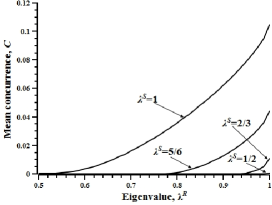
Figure 1: The mean SR-concurrence $\bar{C}$ as a function of $\lambda^{S}$ and $\lambda^{R}$. Each line corresponds to the particular value of $\lambda^{S}=\frac{1}{2},\frac{2}{3},\frac{5}{6},1$ increasing from the bottom to the top of figure. The gridding for averaging: $\alpha_{i},\beta_{i}=0.05n$, $n=0,1,\dots,20$. The same gridding is used in Fig.2. We show only the region $\frac{1}{2}\leq\lambda^{S}\leq 1$, $\frac{1}{2}\leq\lambda^{R}\leq 1$ because of the symmetry $\lambda\leftrightarrow 1-\lambda$.

First of all we shell note that the mean SR-concurrence decreases with an increase in the chain length. It is also an increasing function of both $\lambda^{R}$ and $\lambda^{S}$ reaching its maximal value $\bar{C}_{max}$ at $\lambda^{S}=\lambda^{R}=1$. For the chain of $N=40$ nodes, this maximum is $\bar{C}_{max}=1.15\times 10^{-1}$. Next, the value of $\bar{C}$ tends to zero as $\lambda_{S}\to\frac{1}{2}$ (or $\lambda_{R}\to\frac{1}{2}$) with $\bar{C}|_{\lambda_{S}=\frac{1}{2},\lambda_{R}=1}=\bar{C}|_{\lambda_{S}=1,\lambda_{R}=\frac{1}{2}}=1.87\times 10^{-4}$.

We also observe that all the curves (except the curve $\lambda^{S}=1$) start from some $\lambda^{R}>\frac{1}{2}$. This means that there is a region on the plane of the control parameters $(\lambda^{R},\lambda^{S})$, which maps into the states of the subsystem $SR$ with zero SR-entanglement regardless of the eigenvector control parameters $\tilde{\Gamma}$. This property of our model will be discussed in Sec.IV.1.3 in more details.

IV.1.2 Effect of eigenvector initial parameters $\tilde{\Gamma}$

The effect of $\alpha_{i}$ on $\bar{C}$ is quite similar to that of $\beta_{i}$, $i=1,2$, owing to the symmetry $S\leftrightarrow R$ of the system. Therefore, hereafter in this section we consider only two standard deviations of the SR-concurrence with respect to the parameters $\beta_{i}$, $i=1,2$, using formula (18) with the substitutions $F=C$ and $\gamma=\beta_{i}$:

$$\delta^{(C)}_{\beta_{i}}=\sqrt{\Big{\langle}\Big{(}\bar{C}-\langle C\rangle_{\tilde{\Gamma}_{\beta_{i}}}\Big{)}^{2}\big{\rangle}_{\beta_{i}}},\;\;i=1,2.$$ (36)

These standard deviations are shown in Fig.2. Fig.2a and Fig.2b demonstrate, respectively, that $\bar{C}$ is sensitive to the parameter $\beta_{1}$, and $\bar{C}$ is not sensitive to the parameter $\beta_{2}$. For this reason, the parameters $\alpha_{1}$, $\beta_{1}$ and $\alpha_{2}$, $\beta_{2}$ are referred to as, respectively, strong and weak parameters. We can neglect the effect of $\beta_{2}$ and $\alpha_{2}$ putting $\beta_{2}=\alpha_{2}=0$ in most calculations.

The $\lambda$-dependence of standard deviations $\delta^{(C)}_{\beta_{1}}$ is quite similar to that of the mean concurrence. The function $\delta^{(C)}_{\beta_{2}}$ is different and it is not monotonic with respect to $\lambda^{R}$ and $\lambda^{S}$, which is shown in Fig. 2b. Therewith, unlike the mean concurrence, both $\delta^{(C)}_{\beta_{1}}$ and $\delta^{(C)}_{\beta_{2}}$ vanish at $\lambda^{R}=\frac{1}{2}$, because in this case the receiver’s initial density matrix is proportional to the identity matrix and therefore does not depend on the parameters $\beta_{i}$.

Similar to the mean concurrence, each of the curves in Fig.2a and Fig.2b starts from some $\lambda^{R}>\frac{1}{2}$ (while the curve $\lambda^{S}=1$ starts from $\lambda^{R}=\frac{1}{2}$), which means that there is a region on the $(\lambda^{R},\lambda^{S})$-plane corresponding to the states of the subsystem $SR$ with zero $\delta^{(C)}_{\beta_{1}}$ and $\delta^{(C)}_{\beta_{2}}$. Of cause, the standard deviations are zero in the domain of the $(\lambda^{R},\lambda^{S})$-plane where $\bar{C}=0$, see Sec.IV.1.1. The pre-image of non-entangled states in the control parameter space together with its boundary deserves the special consideration which is given in the next subsection.

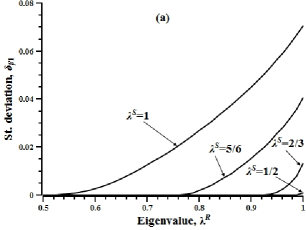
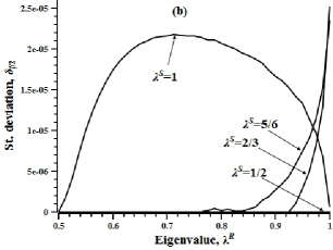
Figure 2: The standard deviations $\delta^{(C)}_{\beta_{i}}$, $i=1,2$, as functions of $\lambda^{S}$ and $\lambda^{R}$. Each line corresponds to the particular value of $\lambda^{S}=\frac{1}{2},\frac{2}{3},\frac{5}{6},1$ increasing from the bottom to the top of figure. Both standard deviations vanish at $\lambda^{R}=\frac{1}{2}$. (a) $\delta^{(C)}_{\beta_{1}}$ with the maximal value $\delta^{(C)}_{\beta_{1}}|_{\lambda^{S}=\lambda^{R}=1}=7.05\times 10^{-2}$. (b) $\delta^{(C)}_{\beta_{2}}$ with the maximal value $\delta^{(C)}_{\beta_{2}}|_{{\lambda^{R}=0.75}\atop{\lambda^{S}=1}}=2.16\times 10^{-5}$,

IV.1.3 Pre-image of non-entangled states $\rho^{SR}$ in control-parameter space and its boundary

In this subsection we disregard the effect of weak control parameters setting $\alpha_{2}=\beta_{2}=0$, which significantly simplifies the numerical calculations.

According to Figs.1 and 2, the SR-concurrence $C$ strongly depends on the control parameters $\lambda^{S}$, $\lambda^{R}$, $\alpha_{1}$ and $\beta_{1}$ and vanishes inside of a large domain of these parameters. In particular, its mean value $\bar{C}$ vanishes if the initial eigenvalues $\lambda^{S}$ and $\lambda^{R}$ are inside of certain domain on the plane $(\lambda^{R},\lambda^{S})$. This domain at $t=43.442$ is shown in Fig.3 and is called the pre-image of non-entangled states $\rho^{SR}$ ($C\equiv 0$) on the plane $(\lambda^{R},\lambda^{S})$.

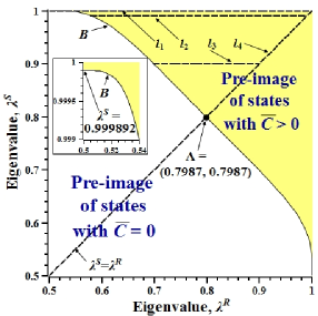
Figure 3: The pre-images of states $\rho^{SR}$ with $\bar{C}=0$ and $\bar{C}>0$ separated by the boundary $B$ on the plane $(\lambda^{R},\lambda^{S})$ at $t=43.442$. The inset represents the boundary $B$ in the close neighborhood of $\lambda^{R}=\frac{1}{2}$ showing the limiting value $\lambda^{S}_{min}=0.999892$ such that, if $\lambda^{S}>\lambda^{S}_{min}$, then $\bar{C}>0$ for all $\lambda^{R}$, $0\leq\lambda^{R}\leq 1$. The boundary $B$ is symmetrical with respect to the bisectrix $\lambda^{S}=\lambda^{R}$, which crosses the boundary at the point $\Lambda=(0.7987,0.7987)$. The pairs of parameters $(\lambda^{R},\lambda^{S})$ along the dashed lines $l_{1}$ – $l_{4}$ (including the bisectrix) will be used for constructing the pre-images of entangled states on the $(\beta_{1},\alpha_{1})$-plane in Fig.6.

We see that there is a well defined boundary (the line $B$) separating the pre-images of the states with $\bar{C}=0$ and $\bar{C}>0$. Furthermore, the inset in this figure shows that there is the limiting value $\lambda^{S}_{min}=0.999892$, such that if $\lambda>\lambda^{S}_{min}$, then the mean SR-concurrence $\bar{C}>0$ for all $\lambda^{R}$, $0\leq\lambda^{R}\leq 1$.

Obviously, the boundary $B$ on the $(\lambda^{R},\lambda^{S})$-plane evolves in time keeping the symmetry with respect to the line $\lambda^{S}=\lambda^{R}$ which is shown in Fig.3. To demonstrate this evolution we take a boundary point $\Lambda$ with the coordinates $\lambda^{S}=\lambda^{R}=0.7987$ (marked in Fig.3) and show its evolution along the bisectrix $\lambda^{S}=\lambda^{R}$ in Fig.4. We see that this point reaches its minimal position at $t=43.442$ (the pre-image of entangled states is above the evolution curve), i.e., exactly at the time instant found for state registration. Therefore, if the initial eigenvalues are taken inside of the domain below the boundary $B$ in Fig.3, then evolution can not create the entangled states irrespective of the values of the eigenvector control-parameters $\alpha_{i}$ and $\beta_{i}$.

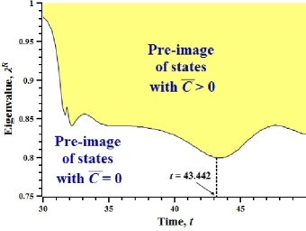
Figure 4: The evolution of the point $\Lambda$ of the boundary $B$ (see Fig.3) along the bisectrix $\lambda^{S}=\lambda^{R}$. The position of $\Lambda$ on the bisectrix is defined by the parameter $\lambda^{R}$ (ordinate axis).

IV.1.4 Witness of SR-entanglement

The numerical simulations show that even if the initial eigenvalues are inside of the pre-image of states with $\bar{C}>0$, the SR-concurrence equals zero in large domain of the control parameters $\alpha_{i}$ and $\beta_{i}$, $i=1,2$. For clarity, we introduce the following witness of SR-entanglement

$$W(\lambda^{S},\lambda^{R})=\int\theta(\lambda^{S},\lambda^{R},\alpha_{1},\beta_{1})d\alpha_{1}d\beta_{1},$$ (37)

where

$$\theta(\Gamma)=\left\{\begin{array}[]{ll}1,&C(\lambda^{S},\lambda^{R},\alpha_{1},\beta_{1})>0\cr 0,&C(\lambda^{S},\lambda^{R},\alpha_{1},\beta_{1})=0\end{array}\right.,$$ (40)

and we take into account that all parameters $\tilde{\Gamma}$ vary inside of the unit interval (13), see Fig.5.

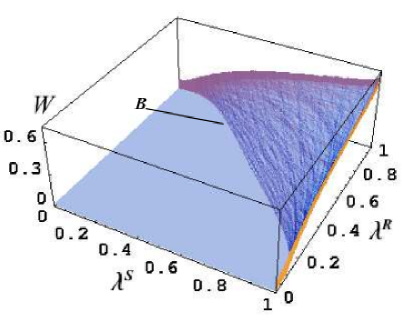
Figure 5: The witness of SR-entanglement $W$ as a function of $\lambda^{R}$ and $\lambda^{S}$ at $t=43.442$.

If the RS-concurrence were nonzero for all values of $\alpha_{1}$ and $\beta_{1}$, then the graph would be horizontal plane with $z$-coordinate equal 1. However, our surface is different and it is always below the above mentioned plane. This means that the SR-concurrence is zero inside of large domain on the plane $(\alpha_{1},\beta_{1})$ and this domain depends on $\lambda^{S}$ and $\lambda^{R}$. Moreover, the slope of the surface in Fig.5 shows that the area of the pre-image of the entangled states on the plane of the parameters $\alpha_{1},\beta_{1}$ increases with the distance from the boundary curve.

IV.1.5 Pre-image of entangled states on $(\beta_{1},\alpha_{1})$-plane

From Fig.5 it follows that the pre-image of entangled states on the plane $(\beta_{1},\alpha_{1})$ depends on the particular values of $\lambda^{S}$ and $\lambda^{R}$. To demonstrate this dependence, we consider the pre-images of the entangled states on the plane $(\beta_{1},\alpha_{1})$, corresponding to different pairs $(\lambda^{R},\lambda^{S})$ taken along the four lines $l_{1}\;-\;l_{4}$ in Fig.3 with

$$\lambda^{S}|_{l_{1}}=1,\;\;\lambda^{S}|_{l_{2}}=0.99,\;\;\lambda^{S}|_{l_{3}}=0.9,\;\;\lambda^{S}|_{l_{4}}=\lambda^{R}.$$ (41)

The results are depicted in Fig.6, where each closed contour is the boundary of the pre-image of entangled states associated with a particular value of the pair $(\lambda^{R},\lambda^{S})$. The smallest central contour (which almost shrinks to a point) in each of Figs. 6b-d corresponds to the point on the appropriate line approaching the boundary $B$ from the right.

The line $l_{1}$ (see Fig.6a) corresponds to the maximal eigenvalue $\lambda^{S}=1$, so that $\lambda^{R}$ runs all the values, $0\leq\lambda^{R}\leq 1$. This figure shows us that there is a rectangular subregion of the pre-image of entangled states for any $\lambda^{R}$ ($0\leq\lambda^{R}\leq 1$): $0\leq\beta_{1}\leq 1,\;\;0\leq\alpha_{1}\leq 0.0763$. If, in addition, $\lambda^{R}=1$, then there are two rectangular subregions of the pre-image of the entangled states:

$${\mbox{1st subregion}}:\;\;0\leq\beta_{1}\leq 1,\;\;0\leq\alpha_{1}\leq 0.0763,$$ (42)

$${\mbox{2nd subregion}}:\;\;0\leq\beta_{1}\leq 0.0763,\;\;0\leq\alpha_{1}<1.$$

The 1st rectangular subregion is the pre-image of states with $\bar{C}>0$ corresponding to $\lambda^{R}=\frac{1}{2}$, i.e., the initial state of the receiver is proportional to the identity matrix and, consequently, doesn’t depend on the parameters $\beta_{i}$. In this case, the SR-entanglement disappears if $\alpha_{1}>0.0763$. Similarly, the 2nd rectangular subregion is the pre-image of states with $\bar{C}>0$ corresponding to $\lambda^{S}=\frac{1}{2}$, the SR-entanglement disappears if $\beta_{1}>0.0763$. Figs.6b-d clearly demonstrate that the area of the pre-image of the entangled states increases with the distance from the boundary $B$ which agrees with Fig.5. Remark that the line, corresponding to $\lambda^{R}=\lambda^{S}=1$, appears in two figures: Fig.6a and Fig.6d.

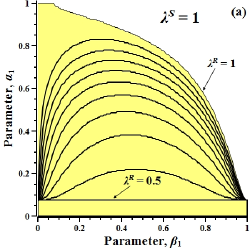
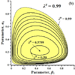
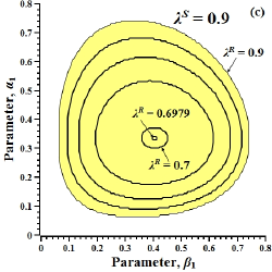
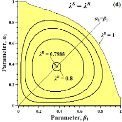
Figure 6: The pre-image of entangled states on the plane $(\beta_{1},\alpha_{1})$ for the eigenvalues $(\lambda^{R},\lambda^{S})$ along the lines $l_{1}$, $l_{2}$, $l_{3}$, $l_{4}$ (see Fig.3). Each curve represents the boundary of the pre-image of entangled states associated with the particular value of $\lambda^{R}$ on the appropriate line $l_{k}$; the $\lambda^{R}$-interval between the neighboring curves is $\Delta\lambda^{R}=0.05$ except the central smallest curves which are specified. All pre-images of the entangled states are simply-connected domains. (a) $\lambda^{S}=1$, $\frac{1}{2}\leq\lambda^{R}\leq 1$ (the line $l_{1}$ in Fig.3). The lower rectangular curve corresponds to $\lambda^{R}=\frac{1}{2}$, the largest curve corresponds to $\lambda^{R}=1$. (b) $\lambda^{S}=0.99$, $0.5799\leq\lambda^{R}\leq 0.99$ (the line $l_{2}$ in Fig.3), the central curve corresponds to $\lambda^{R}=0.5799$, the next one corresponds to $\lambda^{R}=0.59$, the largest curve corresponds to $\lambda^{R}=0.99$. (c) $\lambda^{S}=0.9$, $0.6979\leq\lambda^{R}\leq 0.9$ (the line $l_{3}$ in Fig.3), the central curve corresponds to $\lambda^{R}=0.6979$, the next curve corresponds to $\lambda^{R}=0.7$, the largest curve corresponds to $\lambda^{R}=0.9$, (d) $\lambda^{R}=\lambda^{S}$, $0.7988\leq\lambda^{R}\leq 1$ (the line $l_{4}$ in Fig.3), the central curve corresponds to $\lambda^{R}=0.7988$, the next one corresponds to $\lambda^{R}=0.8$, the largest curve corresponds to $\lambda^{R}=1$.

IV.1.6 Neighborhood of boundary $B$

Finally, we represent the nearest neighborhood of the boundary $B$ on the plane $(\alpha_{1},\beta_{1})$ in Fig.7. This neighborhood corresponds to the line which defers from the boundary line $B$ by the shift $T=0.0001$ along the positive direction of the bisectrix $\lambda^{S}=\lambda^{R}$. This shifted line can be considered as a line of formation of entanglement.

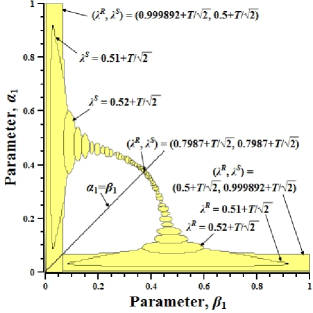
Figure 7: The formation of SR-entanglement on the line neighboring the boundary $B$ in Fig.3. This neighboring line is obtained by shifting the boundary $B$ along the bisectrix $\lambda^{S}=\lambda^{R}$ over $T=0.0001$. Thus, the rectangular contours above the abscissa axis and near the ordinate axis correspond, respectively, to the points $(\lambda^{R},\lambda^{S})=(0.5+\frac{T}{\sqrt{2}},0.999892+\frac{T}{\sqrt{2}})$ and $(\lambda^{R},\lambda^{S})=(0.999892+\frac{T}{\sqrt{2}},0.5+\frac{T}{\sqrt{2}})$. The crosspoint with the bisectrix is $(\lambda^{R},\lambda^{S})=(0.7987+\frac{T}{\sqrt{2}},0.7987+\frac{T}{\sqrt{2}})$. For the two neighboring curves $i$th and $(i+1)$th above and below the bisectrix $\alpha_{1}=\beta_{1}$, we have, respectively, $|\lambda^{S}_{i+1}-\lambda^{S}_{i}|=0.01$, and $|\lambda^{R}_{i+1}-\lambda^{R}_{i}|=0.01$.

IV.2 Informational correlation as function of control parameters

Analyzing the results of Sec.IV.1 we conclude that the SR-concurrence is ”selective” to the values of control parameters and vanishes in large domain of their space. In this section, we show that the informational correlation behaves quite differently.

We study the informational correlation $E^{SR}$ following the strategy of Sec.III.1 and base our consideration on the determinants $\Delta^{(i)}$ instead of $E^{SR}$ itself because they are responsible for the registration of the sender’s control parameters $\alpha_{i}$, $i=1,2$, at the receiver. First, we consider the mean determinants as the functions of eigenvalues $\lambda^{S}$ and $\lambda^{R}$, Sec.IV.2.1, and then we turn to the effects of the eigenvector control parameters in Sec.IV.2.2.

IV.2.1 Mean determinants in dependence on initial eigenvalues

To calculate the mean determinants $\bar{\Delta}^{(i)}$ we use formula (17) with substitutions $F=\Delta^{(i)}$, $i=1,2$. Therewith, $\Delta^{(2)}$ and $\Delta^{(1)}$ are defined, respectively, in eqs. (31) and (32).

Calculating $\bar{\Delta}^{(i)}$, we have to take into account that the dependence of determinants on $\alpha^{(i)}$, $\lambda^{S}$ is separated from their dependence on $\beta^{(i)}$, $\lambda^{R}$ in formulas (31) and (32) (see Appendix, Sec.VII.3 for details). Consequently, formula (17) for the mean determinants $\Delta^{(i)}$ yields:

$$\bar{\Delta}^{(2)}(\lambda^{S},\lambda^{R})=\frac{1}{\Delta^{(2)}_{0}}\sum_{{n,m=1}\atop{m>n}}^{3}\sum_{{i,j=1}\atop{j>i}}^{3}\left\langle\left|\frac{\partial(y_{i},y_{j})}{\partial(x_{n},x_{m})}\right|\right\rangle_{\beta_{1},\beta_{2}}\left\langle\left|\frac{\partial(x_{n},x_{m})}{\partial(\alpha_{1},\alpha_{2})}\right|\right\rangle_{\alpha_{1},\alpha_{2}},$$ (43)

and

$$\bar{\Delta}^{(1)}(\lambda^{S},\lambda^{R})=\frac{1}{\Delta^{(1)}_{0}}\sum_{i,n=1}^{3}\left\langle\left|\frac{\partial y_{i}}{\partial x_{n}}\right|\right\rangle_{\beta_{1},\beta_{2}}\left\langle\left(\left|\frac{\partial x_{n}}{\partial\alpha_{1}}\right|+\left|\frac{\partial x_{n}}{\partial\alpha_{2}}\right|\right)\right\rangle_{\alpha_{1},\alpha_{2}}$$ (44)

Moreover, the averaging over $\alpha_{i}$ can be simply done analytically, i.e.,

$$\left\langle\left|\frac{\partial(x_{n},x_{m})}{\partial(\alpha_{1},\alpha_{2})}\right|\right\rangle_{\alpha_{1},\alpha_{2}}=\frac{\pi}{2}(1-2\lambda^{S})^{2},\;\;(n,m)=(1,2),(1,3),(2,3)$$ (45)

and

$$\left\langle\left(\left|\frac{\partial x_{n}}{\partial\alpha_{1}}\right|+\left|\frac{\partial x_{n}}{\partial\alpha_{2}}\right|\right)\right\rangle_{\alpha_{1},\alpha_{2}}=\left\{\begin{array}[]{ll}|1-2\lambda^{S}|,&n=1\cr\frac{6}{\pi}|1-2\lambda^{S}|,&n=2,3.\end{array}\right.$$ (48)

The mean determinants $\bar{\Delta}^{(i)}$, $i=1,2$, as functions of $\lambda^{S}$ and $\lambda^{R}$ are depicted in Fig. 8

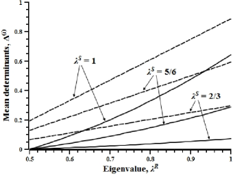
Figure 8: The mean determinants $\bar{\Delta}^{(2)}$ (solid line) and $\bar{\Delta}^{(1)}$ (dashed line) as functions of $\lambda^{S}$ and $\lambda^{R}$. Each line corresponds to the particular value of $\lambda^{S}=\frac{1}{2},\frac{2}{3},\frac{5}{6},1$ increasing from the bottom to the top of the figure with $\bar{\Delta}^{2}|_{\lambda^{S}=\frac{1}{2}}=\bar{\Delta}^{1}|_{\lambda^{S}=\frac{1}{2}}=0$. Each function $\bar{\Delta}^{(2)}$ and $\bar{\Delta}^{(1)}$ takes its maximal value at the boundary point $\lambda^{S}=\lambda^{R}=1$: $\bar{\Delta}^{(2)}_{\max}=0.6413$ and $\bar{\Delta}^{(1)}_{\max}=0.8869$. Therewith, $\bar{\Delta}^{(2)}$ turns to zero at $\lambda^{R}=\frac{1}{2}$ for all $\lambda^{S}$. On the contrary, $\bar{\Delta}^{(1)}$ doesn’t vanish at $\lambda^{R}=\frac{1}{2}$, its maximal value in this case is at $\lambda^{S}=1$: $\bar{\Delta}^{(1)}|_{{\lambda^{S}=1}\atop{\lambda^{R}=\frac{1}{2}}}=0.1929$.

We see that, unlike the concurrence, there is no domain on the plane $(\lambda^{R},\lambda^{S})$ resulting in the zero mean determinants. Both of them vanish on the line $\lambda^{S}=\frac{1}{2}$ (any $\lambda^{R}$), and in addition $\bar{\Delta}^{(2)}$ vanishes on the line $\lambda^{R}=\frac{1}{2}$ (any $\lambda^{S}$). Moreover, there is no domain on the plane $(\alpha_{1},\beta_{1})$ leading to the vanishing determinants. There are only two lines $\alpha_{1}=0$ and $\alpha_{1}=1$ (any $\beta_{1}$, $\alpha_{2}$ and $\beta_{2}$ ) yielding the zero determinant $\Delta^{(2)}$, while $\Delta^{1}\neq 0$ for any initial parameters $\alpha_{i}$ and $\beta_{i}$ (if $\lambda^{S}\neq\frac{1}{2}$).

IV.2.2 Effect of eigenvector initial parameters $\tilde{\Gamma}$

Unlike the concurrence, the informational correlation is not symmetrical with respect to the replacement $S\leftrightarrow R$, and so do the determinants $\Delta^{(i)}$ ($i=1,2$). Therefore, we consider the four standard deviations for each determinant $\Delta^{(i)}$:

$$\delta^{\Delta^{(i)}k}_{\beta_{i}}\equiv\delta^{(k)}_{\beta_{i}}=\sqrt{\Big{\langle}\Big{(}\bar{\Delta}^{(k)}-\langle\Delta^{(k)}\rangle_{\tilde{\Gamma}_{\beta_{i}}}\Big{)}^{2}\big{\rangle}_{\beta_{i}}},\;\;i,k=1,2,$$ (49)

$$\delta^{\Delta^{(i)}k}_{\alpha_{i}}\equiv\delta^{(k)}_{\alpha_{i}}=\sqrt{\Big{\langle}\Big{(}\bar{\Delta}^{(k)}-\langle\Delta^{(k)}\rangle_{\tilde{\Gamma}_{\alpha_{i}}}\Big{)}^{2}\big{\rangle}_{\alpha_{i}}},\;\;i,k=1,2.$$ (50)

The standard deviations $\delta^{(k)}_{\beta_{i}}$ are shown in Fig.9. We see similarity in their behavior. Fig.9a demonstrates that determinants $\bar{\Delta}^{(i)}$ ($i=1,2$) are sensitive to the parameter $\beta_{1}$ (strong parameter), while, according to Fig.9b, they are non-sensitive to the parameter $\beta_{2}$ (weak parameter).

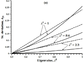
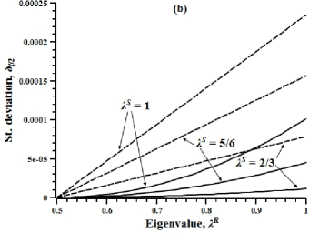
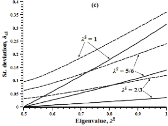
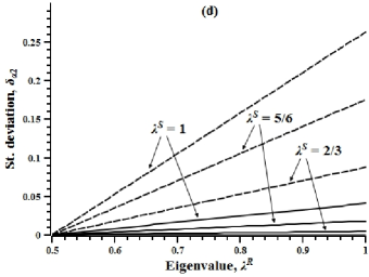
Figure 9: The standard deviations $\delta^{(2)}_{\beta_{i}}$, $\delta^{(2)}_{\alpha_{i}}$ (solid lines) and $\delta^{(1)}_{\beta_{i}}$, $\delta^{(1)}_{\alpha_{i}}$ (dashed lines), $i=1,2$, as functions of $\lambda^{R}$ and $\lambda^{S}$. Each line corresponds to the particular value of $\lambda^{S}=\frac{1}{2},\frac{2}{3},\frac{5}{6},1$ increasing from the bottom to the top of the figure with ${\delta}^{2}_{\gamma}|_{\lambda^{S}=\frac{1}{2}}\equiv{\delta}^{1}_{\gamma}|_{\lambda^{S}=\frac{1}{2}}=0$ ($\gamma=\alpha_{i},\beta_{i}$). In addition, all the standard deviations vanish at $\lambda^{R}=\frac{1}{2}$ except $\delta^{(1)}_{\alpha_{1}}$. (a) $\delta^{(k)}_{\beta_{1}}$, $k=1,2$, with their maximal values $\delta^{(2)}_{\beta_{1}}|_{\lambda^{S}=\lambda^{R}=1}=0.3584$, $\delta^{(1)}_{\beta_{1}}|_{\lambda^{S}=\lambda^{R}=1}=0.3322$. (b) $\delta^{(k)}_{\beta_{2}}$, $k=1,2$, with their maximal values $\delta^{(2)}_{\beta_{2}}|_{\lambda^{S}=\lambda^{R}=1}=1.008\times 10^{-4}$, $\delta^{(1)}_{\beta_{2}}|_{\lambda^{S}=\lambda^{R}=1}=2.344\times 10^{-4}$. (c) $\delta^{(k)}_{\alpha_{1}}$, $k=1,2$, with their maximal values $\delta^{(2)}_{\alpha_{1}}|_{\lambda^{S}=\lambda^{R}=1}=0.3137$, $\delta^{(1)}_{\alpha_{1}}|_{\lambda^{S}=\lambda^{R}=1}=0.3601$. In addition, $\delta^{(1)}_{\alpha_{1}}|_{{\lambda^{R}=\frac{1}{2}}\atop{\lambda^{S}=1}}=9.477\times 10^{-2}$. (d) $\delta^{(k)}_{\alpha_{2}}$, $k=1,2$, with their maximal values $\delta^{(2)}_{\alpha_{2}}|_{\lambda^{S}=\lambda^{R}=1}=4.067\times 10^{-2}$, $\delta^{(1)}_{\alpha_{2}}|_{\lambda^{S}=\lambda^{R}=1}=0.2630$.

As shown in Fig.9c,d, both $\alpha_{1}$ and $\alpha_{2}$ are strong parameters (i.e., they significantly effect the determinants), contrary to the case of SR-entanglement.

Remark, that all the standard deviations vanish at $\lambda^{R}=\frac{1}{2}$, except $\delta^{(1)}_{\alpha_{1}}$. Therefore, the control parameter $\alpha_{1}$ of the sender can be considered as the strongest one.

Remember that the informational correlation $E^{SR}$ discussed above depends on the direction of the information transfer (from the sender to the receiver). Reversing this direction, we change the strong and weak eigenvector parameters. Thus, in $E^{SR}$, the strong parameters are $\alpha_{i}$, $i=1,2$, and $\beta_{1}$, while $\beta_{2}$ is a weak one. On the contrary, in $E^{RS}$, the strong parameters are $\beta_{i}$, $i=1,2$, and $\alpha_{1}$, while $\alpha_{2}$ is a weak one.

V Comparative analysis of SR-entanglement and informational correlation

Now we compare the SR-concurrence and determinants as functions of control parameters. As was clearly demonstrated in Sec.IV.1.3, if the initial eigenvalues $\lambda^{S}$ and $\lambda^{R}$ are below the boundary $B$ (see Fig.3), then the SR-entanglement can not appear during the evolution regardless of the values of the control parameters $\alpha_{i}$ and $\beta_{i}$. Moreover, if the initial eigenvalues $\lambda^{S}$ and $\lambda^{R}$ are above the boundary $B$, then the SR-entanglement can still be zero at the registration instant unless we take the proper values of the control parameters $\alpha_{1}$ and $\beta_{1}$. In the case of perfect state transfer, the boundary $B$ shrinks to the point $(\lambda^{R},\lambda^{S})=(\frac{1}{2},\frac{1}{2})$.

Meanwhile, the mean determinants $\bar{\Delta}^{(i)}$ do not vanish both above and below the boundary $B$ (except the particular lines found in Sec. IV.2); therefore the eigenvector parameters $\alpha_{i}$ of the sender’s state can be transferred to the receiver even if there is no entanglement between these subsystems during the evolution. All this demonstrates that the SR-entanglement is not responsible for information propagation and remote state creation because it vanishes in large domain of the control parameters. On the contrary, the informational correlation is more suitable measure of quantum correlations in this case.

Comparing Fig. 1 with Fig. 8 at $\lambda^{R}=\frac{1}{2}$, we see that $\bar{C}$ doesn’t vanish, although its value is very small with the maximum $\bar{C}|_{\lambda^{S}=1}=1.87\times 10^{-4}$. Meanwhile, $\Delta^{(2)}=0$ and $\Delta^{(1)}\neq 0$ with the maximal value $\bar{\Delta}^{(1)}|_{\lambda^{S}=1}=0.1929.$ Thus we can say that the mean SR-entanglement is non-zero identically if at least one of the eigenvector parameters can be transferred from the sender to the receiver.

We also see that the mean values of both SR-concurrence and determinants are small in the neighborhood of $\lambda^{R}=\frac{1}{2}$. This means that the problem of small concurrence appearing in our model, in certain sense, is equivalent to the problem of small determinants in linear algebra.

VI Conclusions

We study the dependence of entanglement and informational correlation between the two remote one-qubit subsystems $S$ and $R$ on the control parameters (which are the parameters of the sender and receiver initial states). The entanglement is the well known measure responsible for many advantages of quantum information devices in comparison with their classical counterparts. The informational correlation, being based on the parameter exchange between the sender and receiver, is closely related to the remote mixed state creation. Our basic results are are following.

1. There are strong eigenvector control-parameters which can significantly change the quantum correlations. In the case of concurrence, these are $\alpha_{1}$ and $\beta_{1}$. In the case of informational correlation, there are three such parameters: $\alpha_{1}$, $\alpha_{2}$ and $\beta_{1}$ for $E^{SR}$ and $\beta_{1}$, $\beta_{2}$ and $\alpha_{1}$ for $E^{RS}$. Other eigenvector control-parameters are weak, they do not essentially effect the quantum correlations. These are parameters $\alpha_{2}$ and $\beta_{2}$ in the case of concurrence. As for the informational correlation, there is only one weak parameter: $\beta_{2}$ for $E^{SR}$ and $\alpha_{2}$ for $E^{RS}$.

2. The eigenvalues are most important parameters which strongly effect the quantum correlations and, in principle, they might be joined to the above strong control parameters. However, we keep them in a different group to emphasize the difference between the eigenvector- and eigenvalue control parameters.

3. In certain sense, there is an equivalence between the problem of vanishing entanglement and the problem of vanishing determinants in linear algebra.

4. There is a large domain in the control parameter space mapped into the non-entangled states. On the contrary, there is no domain in the control-parameter space leading to zero determinants. The determinants vanish only for exceptional values of the control parameters. This fact promotes the informational correlation for a suitable quantity describing the quantum correlations responsible for the state transfer/creation.

5. It is remarkable that the weak parameters not only slightly effect on the SR-entanglement and determinants, but have a distinguished feature in the problem of remote state creation. Namely, according to Z_2014 ; BZ_2015 , any value of the weak parameter can be created in the receiver’s state using the proper value of the weak parameter of the sender. Therefore, the weak parameters can be used for organization of the effective information transfer without changing the value of SR-entanglement.

Authors thank Prof. E.B.Fel’dman for useful discussion. This work is partially supported by the Program of the Presidium of RAS ”Element base of quantum computers”(No. 0089-2015-0220) and by the Russian Foundation for Basic Research, grant No.15-07-07928.

VII Appendix

VII.1 Permanent characteristics of communication line

Writing $\rho^{SR}$ (14) in components, we have

$$\rho^{SR}_{i_{1}i_{N};j_{1}j_{N}}=T_{i_{1}i_{N}l_{1}l_{N};j_{1}j_{N}k_{1}k_{N}}(\rho^{S}_{0})_{l_{1};k_{1}}(\rho^{R}_{0})_{l_{N};k_{N}}.$$ (51)

Here all the indexes take two values $0$ and $1$, the parameters $T_{i_{1}i_{N}l_{1}l_{N};j_{1}j_{N}k_{1}k_{N}}$ in this formula depend on the Hamiltonian as follows:

$$T_{i_{1}i_{N}l_{1}l_{N};j_{1}j_{N}k_{1}k_{N}}=\sum_{i_{TL},l_{TL},k_{TL}}V_{i_{1}i_{TL}i_{N};l_{1}l_{TL}l_{N}}\rho^{TL}_{l_{TL};k_{TL}}V^{+}_{k_{1}k_{TL}k_{N};j_{1}i_{TL}j_{N}},$$ (52)

where the indexes with the subscript $TL$ are the vector indexes of $(N-2)$ scalar binary indexes, for instance: $i_{TL}=\{i_{2}\dots i_{N-1}\}$. We refer to these parameters as $T$-parameters. In formulas (51) and (52), we write the components of both the density matrices and the operator $V$, where both rows and columns are enumerated by the vector subscripts consisting of the binary indexes. For instance,

$$\rho^{SR}_{i_{1}i_{N};j_{1}j_{N}}\;\;{\mbox{is the element at the intersection of row}}\;\;\{i_{1}i_{N}\}\;\;{\mbox{and column}}\;\;\{j_{1}j_{N}\},$$

and similar for the components of the operator $V$.

If the transmission line is in ground state (2), then the expression for the $T$-parameters is simpler:

$$T_{i_{1}i_{N}l_{1}l_{N};j_{1}j_{N}k_{1}k_{N}}=\sum_{i_{TL}}V_{i_{1}i_{TL}i_{N};l_{1}0_{TL}l_{N}}V^{+}_{k_{1}0_{TL}k_{N};j_{1}i_{TL}j_{N}},$$ (53)

where $0_{TL}=(\underbrace{0,\dots,0}_{N-2})$. The number of $T$-parameters is independent on the length of a transmission line and is completely defied by the dimensionality of the sender and receiver.

The $T$-parameters have two obvious symmetries. The first one follows from the Hermitian property of the density matrix (51), $(\rho^{SR})^{+}=\rho^{SR}$:

$$T_{i_{1}i_{N}l_{1}l_{N};j_{1}j_{N}k_{1}k_{N}}=T_{j_{1}j_{N}k_{1}k_{N};i_{1}i_{N}l_{1}l_{N}}^{*}\;\;\Rightarrow\;\;{\mbox{Im}}\;T_{j_{1}j_{N}k_{1}k_{N};j_{1}j_{N}k_{1}k_{N}}=0.$$ (54)

The second symmetry follows from the fact that these parameters must be symmetrical with respect to the exchange $S\leftrightarrow R$:

$$T_{i_{1}i_{N}l_{1}l_{N};j_{1}j_{N}k_{1}k_{N}}=T_{i_{N}i_{1}l_{N}l_{1};j_{N}j_{1}k_{N}k_{1}}.$$ (55)

Finally, the set of $T$-parameters equals zero as a consequence of the fact that the Hamiltonian commutes with the $z$-projection of the total momentum $I_{z}$; therefore the nonzero elements $V_{I,J}$ of the evolution operator are those, whose $N$-dimensional vector indexes $I$ and $J$ have equal number of units. Consequently (if the transmission line $TL$ is in ground state (2) initially),

$$T_{i_{1}i_{N}l_{1}l_{N};j_{1}j_{N}k_{1}k_{N}}=0\;\;{\mbox{if}}\;\;\left\{\begin{array}[]{l}i_{1}+i_{N}>l_{1}+l_{N}\cr j_{1}+j_{N}>k_{1}+k_{N}\cr i_{1}+i_{N}<l_{1}+l_{N}\;\;{\mbox{and}}\;\;i_{1}+i_{N}-(j_{1}+j_{N})\neq l_{1}+l_{N}-(k_{1}+k_{N})\end{array}\right..$$ (59)

In other words, the following $T$-parameters are nonzero:

$$T_{i_{1}i_{N}l_{1}l_{N};j_{1}j_{N}k_{1}k_{N}}\neq 0\;\;{\mbox{if}}\;\;$$ (60)

$$(i_{1}+i_{N}\leq l_{1}+l_{N})\wedge(j_{1}+j_{N}\leq k_{1}+k_{N})\wedge(i_{1}+i_{N}-j_{1}-j_{N}=l_{1}+l_{N}-k_{1}-k_{N}).$$

The $T$-parameters are permanent characteristics of the communication line which do not change during its operation.

VII.2 Explicit form for elements of receiver’s density matrix

We obtain the element of the receiver’s density matrix $\rho^{R}(t)$ calculating the trace of the matrix $\rho^{SR}$ (51) over the sender’s node:

$$\rho^{R}_{i_{N};j_{N}}=\sum_{i_{1},j_{1}}\rho^{SR}_{i_{1}i_{N};j_{1}j_{N}}=T_{i_{N}l_{1};j_{N}k_{1}}(\rho^{S}_{0})_{l_{1};k_{1}},$$ (61)

where

$$T_{i_{N}l_{1};j_{N}k_{1}}=\sum_{l_{N},k_{N},i_{1}}T_{i_{1}i_{N}l_{1}l_{N};i_{1}j_{N}k_{1}k_{N}}(\rho^{R}_{0})_{l_{N};k_{N}},$$ (62)

and $T_{i_{N}l_{1};j_{N}k_{1}}$ satisfies the symmetry following from symmetry (54):

$$T_{i_{N}l_{1};j_{N}k_{1}}=T_{j_{N}k_{1};i_{N}l_{1}}^{*}\;\;\Rightarrow\;\;{\mbox{Im}}\;T_{i_{N}l_{1};i_{N}l_{1}}=0.$$ (63)

In result, the independent elements of $\rho^{R}$ read as follows:

$$\rho^{R}_{1;1}=T_{10;10}+(T_{11;11}-T_{10;10})x_{1}+(T_{10;11}+T_{11;10})x_{2}+i(T_{10;11}-T_{11;10})x_{3},$$ (64)

$$\rho^{R}_{0;1}=T_{00;10}+(T_{01;11}-T_{00;10})x_{1}+(T_{00;11}+T_{01;10})x_{2}+i(T_{00;11}-T_{01;10})x_{3},$$ (65)

which is a system of linear algebraic equations allowing us to determine the initial parameters $x_{i}$ knowing the registered density matrix of the receiver’s state. We can conveniently rewrite system (64) separating the real and imaginary parts to get three independent real equations (30).

VII.3 Some properties of determinants

The both determinants $\Delta^{(1)}$ and $\Delta^{(2)}$ depend on the parameters of the initial states of the sender and receiver: $\lambda^{S}$, $\lambda^{R}$, $\alpha_{i}$, $\beta_{i}$, $i=1,2$. But this dependence is partially separated, which has been already used in eqs.(34): expressions $\left|\frac{\partial(y_{i},y_{j})}{\partial(x_{n},x_{m})}\right|$ and $\left|\frac{\partial y_{i}}{\partial x_{n}}\right|$ in, respectively, eqs.(31) and (32) depend on $\lambda^{R}$, $\beta_{i}$, $i=1,2$, while expressions $\left|\frac{\partial(x_{n},x_{m})}{\partial(\alpha_{1},\alpha_{2})}\right|$ and $\left(\left|\frac{\partial x_{n}}{\partial\alpha_{1}}\right|+\left|\frac{\partial x_{n}}{\partial\alpha_{2}}\right|\right)$ in, respectively, eqs.(31) and (32) depend on $\lambda^{S}$, $\alpha_{i}$, $i=1,2$. All this immediately follows from the definitions of $x_{i}$ (29) and elements of $\rho^{R}$ (30).

Notice that each term in definitions (32) and (31) is the independent determinant condition for solvability of system (30) for, respectively, two parameters $\alpha_{i}$, $i=1,2$, or one of them. In other words, if there are $k$ nonzero terms in these formulas, then we can find parameters $\alpha_{i}$ ($i=1,2$) in $k$ different ways. In principle, if each term is small in eq.(31) (or (32)), then the parameters $\alpha_{1}$ and $\alpha_{2}$ (or one of them) can be found from system (30) with restricted accuracy. However, if there are $k$ small but nonzero terms in (32) (or (31)), then the accuracy can be improved by calculating the transferred parameters $k$ times and comparing the results. For this reason we do not divide the sums in both formulas (32) and (31) by the number of terms in them.

VII.4 Choice of time instant for state registration

Now we show that $C$ and the determinants $\Delta^{(i)}$ averaged over the initial conditions are maximal at the time instant of the maximum of $\langle\bar{P}\rangle_{\lambda^{S},\lambda^{R}}(t)=\bar{P}(t)$, where

$$\bar{P}(t) \equiv \langle P\rangle_{\tilde{\Gamma}}=\frac{1}{P_{0}}\left\langle\rho^{(SR)}_{01;01}(t)+\rho^{(SR)}_{10;10}(t)+\rho^{(SR)}_{11;11}(t)\right\rangle_{\tilde{\Gamma}}=$$

$$\frac{2}{3}\left(T_{0110;0110}(t)+T_{1010;1010}(t)+T_{1011;1011}(t)+\frac{1}{2}T_{1111;1111}(t)\right).$$

Here $P_{0}=\frac{3}{4}$ is the normalization fixed by the requirement $\bar{P}|_{t=0}=1$ and we take into account that $\bar{P}$ doesn’t depend on the initial eigenvalues $\lambda^{S}$ and $\lambda^{R}$. The function $P$ can be viewed as a probability of registration of the excitation at the nodes of the subsystem $SR$. The numerical calculations show that its maximum coincides with the maximum of fidelity of a one-qubit pure state transfer:

$$\bar{P}^{R}(t)=\rho^{(SR)}_{01;01}(t)|_{\Gamma=\{0,1,0,0,0,0\}}=T_{0110;0110}(t).$$ (67)

This fact simplifies our calculations.

The time-dependences of the functions $\langle\bar{P}\rangle_{\lambda^{S},\lambda^{R}}\equiv\bar{P}$, $\langle\bar{\Delta}^{(i)}\rangle_{\lambda^{S},\lambda^{R}}$ and $\langle\bar{C}\rangle_{\lambda^{S},\lambda^{R}}$ are shown in Fig. 10 for the chain of $N=40$ nodes (for convenience, we normalize them by their maxima over the considered long enough interval, $0\leq t\leq 50$ , i.e., we show the ratios

$$\langle{P}\rangle_{n}=\frac{\langle\bar{P}\rangle_{\lambda^{S},\lambda^{R}}}{\langle\bar{P}\rangle_{\lambda^{S},\lambda^{R}}^{max}},\;\;\langle{C}\rangle_{n}=\frac{\langle\bar{C}\rangle_{\lambda^{S},\lambda^{R}}}{\langle\bar{C}\rangle_{\lambda^{S},\lambda^{R}}^{max}},\;\;\langle{\Delta}^{(i)}\rangle_{n}=\frac{\langle\bar{\Delta}^{(i)}\rangle_{\lambda^{S},\lambda^{R}}}{\langle\bar{\Delta}^{(i)}\rangle_{\lambda^{S},\lambda^{R}}^{max}},$$ (68)

where

$$\langle\bar{P}\rangle_{\lambda^{S},\lambda^{R}}^{max}=\langle\bar{P}\rangle_{\lambda^{S},\lambda^{R}}|_{t=43.442}=0.5476,\;\;\langle\bar{C}\rangle_{\lambda^{S},\lambda^{R}}^{max}=\langle\bar{C}\rangle_{\lambda^{S},\lambda^{R}}|_{t=43.442}=9.584\times 10^{-3},$$ (69)

$$\langle\bar{\Delta}^{(2)}\rangle_{\lambda^{S},\lambda^{R}}^{max}=\langle\bar{\Delta}^{(2)}\rangle_{\lambda^{S},\lambda^{R}}|_{t=43.442}=9.846\times 10^{-2},\;\;\langle\bar{\Delta}^{(1)}\rangle_{\lambda^{S},\lambda^{R}}^{max}=\langle\bar{\Delta}^{(1)}\rangle_{\lambda^{S},\lambda^{R}}|_{t=43.442}=0.2765.$$

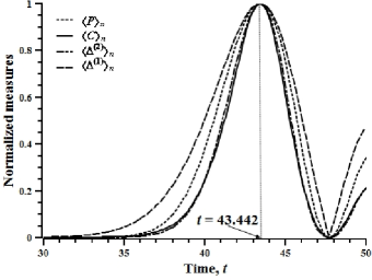
Figure 10: The time-dependence of the normalized mean probability $\langle\bar{P}\rangle_{n}$ (dotted line), mean SR-concurrence $\langle\bar{C}\rangle_{n}$ (solid line), mean determinants $\langle\bar{\Delta}^{(2)}\rangle_{n}$ (dash-dotted line) and $\langle\bar{\Delta}^{(1)}\rangle_{n}$ (dashed line) defined in eq.(68) with normalizations given in (69). All four curves have the maximum at the same time instant $t=43.442$ (we use the values of $T$-parameters found in Appendix, Sec.VII.5).

We see that the time instant of the maxima is the same for all four functions and equals $t=43.442$. Namely this optimized time instant is taken for our calculations.

VII.5 Numerical values of $T$-parameters for $N=40$ at optimized time instant.

For the case $N=40$, we have calculated the $T$-parameters at the optimized time instant $t=43.442$ found in Sec.VII.4. Similar to SZ_2016 , the $T$-parameters can be separated into three families by their absolute values. We give the list of these families up to symmetries (54,55).

1st family: There are two different parameters with the absolute values gapped in the interval $[6.817\times 10^{-1},1]$:

$$T_{0000;0000}=1,T_{0000;0110}=-6.817i\times 10^{-1}.$$ (70)

2nd family: There are 8 different parameters with the absolute values gapped in the interval $[2.160\times 10^{-1},5.353\times 10^{-1}]$:

$$T_{0001;0001}=5.352\times 10^{-1},\;\;T_{0011;0011}=2.865\times 10^{-1},\;\;$$ (71)

$$T_{0001;0111}=3.649i\times 10^{-1},\;\;T_{0000;1111}=4.648\times 10^{-1},\;\;$$

$$T_{0110;0110}=4.648\times 10^{-1},\;\;T_{0111;0111}=2.488\times 10^{-1},\;\;$$

$$T_{0110;1111}=3.169i\times 10^{-1},\;\;T_{1111;1111}=2.160\times 10^{-1}.$$

3rd family: There are 5 different parameters with the absolute values gapped in the interval $[0,5.396\times 10^{-3}]$:

$$T_{0000;0101}=-5.395\times 10^{-3},\;\;T_{0010;0111}=-2.888\times 10^{-3},$$ (72)

$$T_{0101;0101}=2.911\times 10^{-5},\;\;T_{0101;0110}=3.678i\times 10^{-3},$$

$$T_{0101;1111}=-2.508\times 10^{-3}.$$

Notice that the parameter $T_{0001;0010}$ vanishes only due to the nearest-neighbor interaction model and/or even $N$. It becomes non-vanishing if at least one of these conditions is destroyed.

We see that there are certain gaps between the neighboring families, which is most significant ($\sim 10^{2}$) between the 2nd and the 3rd families. In addition, the parameters from the 3rd family are smallest ones. Similar to ref.SZ_2016 , this difference in absolute values of the $T$-parameters is due to the symmetries of transitions among the different nodes of the chain. The obtained values of the $T$-parameters are used in Sec.IV.2.

References

- (1) S.Hill and W.K.Wootters, Phys. Rev. Lett. 78, 5022 (1997)
- (2) W.K. Wootters, Phys. Rev. Lett. 80, 2245 (1998)
- (3) Bennett, C.H., DiVincenzo, D.P., Fuchs, C.A., Mor, T., Rains, E., Shor, P.W., Smolin, J.A., Wootters, W.K., Phys. Rev. A 59, 1070 (1999)
- (4) Horodecki, M., Horodecki, P., Horodecki, R., Oppenheim, J., Sen, A., Sen, U., Synak-Radtke, B., Phys. Rev. A 71, 062307 (2005)
- (5) Niset, J., Cerf, N.J., Phys. Rev. A 74, 052103 (2006)
- (6) Meyer, D.A. Phys. Rev. Lett. 85, 2014 (2000)
- (7) A.Datta, A.Shaji, C.M.Caves, Phys.Rev.Lett. 100, 050502 (2008)
- (8) Datta, A., Flammia, S.T., Caves, C.M., Phys. Rev. A 72, 042316 (2005)
- (9) Datta, A., Vidal, G., Phys. Rev. A 75, 042310 (2007)
- (10) B.P.Lanyon, M.Barbieri, M.P.Almeida, A.G.White, Phys.Rev.Lett. 101, 200501 (2008)
- (11) W. H. Zurek, Ann. Phys.(Leipzig), 9, 855 (2000)
- (12) L.Henderson and V.Vedral J.Phys.A:Math.Gen. 34, 6899 (2001)
- (13) H.Ollivier, W.H.Zurek, Phys. Rev. Lett. 88, 017901 (2001)
- (14) W. H. Zurek, Rev. Mod. Phys. 75, 715 (2003)
- (15) M.Zukowski, A.Zeilinger, M.A.Horne, A.K.Ekert, Phys. Rev. Lett. 71, 4287 (1993)
- (16) D.Bouwmeester, J.-W. Pan, K.Mattle, M.Eibl, H.Weinfurter, and A. Zeilinger, Nature 390, 575 (1997)
- (17) D. Boschi, S. Branca, F. De Martini, L. Hardy, and S. Popescu, Phys. Rev. Lett. 80, 1121 (1998)
- (18) N.A.Peters, J.T.Barreiro, M.E.Goggin, T.-C.Wei, and P.G.Kwiat, Phys.Rev.Lett. 94, 150502 (2005)
- (19) N.A.Peters, J.T.Barreiro, M.E.Goggin, T.-C.Wei, and P.G.Kwiat in Quantum Communications and Quantum Imaging III, ed. R.E.Meyers, Ya.Shih, Proc. of SPIE 5893 (SPIE, Bellingham, WA, 2005)
- (20) B.Dakic, Ya.O.Lipp, X.Ma, M.Ringbauer, S.Kropatschek, S.Barz, T.Paterek, V.Vedral, A.Zeilinger, C.Brukner, and P.Walther, Nat. Phys. 8, 666 (2012).
- (21) G.Y. Xiang, J.Li, B.Yu, and G.C.Guo Phys. Rev. A 72, 012315 (2005)
- (22) L.L.Liu, T. Hwang, Quantum Inf. Process. 13, 1639 (2014)
- (23) S. Bose, Phys. Rev. Lett. 91, 207901 (2003)
- (24) M.Christandl, N.Datta, A.Ekert and A.J.Landahl, Phys.Rev.Lett. 92, 187902 (2004)
- (25) C.Albanese, M.Christandl, N.Datta and A.Ekert, Phys.Rev.Lett. 93, 230502 (2004)
- (26) P.Karbach and J.Stolze, Phys.Rev.A 72, 030301(R) (2005)
- (27) G.Gualdi, V.Kostak, I.Marzoli and P.Tombesi, Phys.Rev. A 78, 022325 (2008)
- (28) A.Wójcik, T.Luczak, P.Kurzyński, A.Grudka, T.Gdala, and M.Bednarska Phys. Rev. A 72, 034303 (2005)
- (29) G.M.Nikolopoulos and I.Jex, eds., Quantum State Transfer and Network Engineering, Series in Quantum Science and Technology, Springer, Berlin Heidelberg (2014)
- (30) J.Stolze, G. A. Álvarez, O. Osenda, A. Zwick in Quantum State Transfer and Network Engineering. Quantum Science and Technology, ed. by G.M.Nikolopoulos and I.Jex, Springer Berlin Heidelberg, Berlin, p.149 (2014)
- (31) B. Chen and Zh. Song, Sci. China-Phys., Mech.Astron. 53, 1266 (2010).
- (32) C. A. Bishop, Yo.-Ch. Ou, Zh.-M. Wang, and M. S. Byrd, Phys. Rev. A 81, 042313 (2010)
- (33) T. J. G. Apollaro, L. Banchi, A. Cuccoli, R. Vaia, and P. Verrucchi, Phys. Rev. A 85, 052319 (2012)
- (34) A.I.Zenchuk, J. Phys. A: Math. Theor. 45 (2012) 115306
- (35) A.I.Zenchuk, Quant. Inf. Proc. 13, 2667-2711 (2014)
- (36) E. B. Fel’dman , M. A. Yurishchev, JETP Letters 90, 70 (2009)
- (37) M. A. Yurishchev, JETP 111, 525 (2010)
- (38) J.Stolze, A.I.Zenchuk, to appear in Quant.Inf.Proc. 15, 3347-3366 (2016) arXiv:1512.04309
- (39) A.I.Zenchuk, Phys. Rev. A 90, 052302(13) (2014)
- (40) G. A. Bochkin and A. I. Zenchuk, Phys.Rev.A 91, 062326(11) (2015)