Assessing Percolation Threshold Based on High-Order Non-Backtracking Matrices

Abstract

Percolation threshold of a network is the critical value such that when nodes or edges are randomly selected with probability below the value, the network is fragmented but when the probability is above the value, a giant component connecting a large portion of the network would emerge. Assessing the percolation threshold of networks has wide applications in network reliability, information spread, epidemic control, etc. The theoretical approach so far to assess the percolation threshold is mainly based on spectral radius of adjacency matrix or non-backtracking matrix, which is limited to dense graphs or locally treelike graphs, and is less effective for sparse networks with non-negligible amount of triangles and loops. In this paper, we study high-order non-backtracking matrices and their application to assessing percolation threshold. We first define high-order non-backtracking matrices and study the properties of their spectral radii. Then we focus on the 2nd-order non-backtracking matrix and demonstrate analytically that the reciprocal of its spectral radius gives a tighter lower bound than those of adjacency and standard non-backtracking matrices. We further build a smaller size matrix with the same largest eigenvalue as the 2nd-order non-backtracking matrix to improve computation efficiency. Finally, we use both synthetic networks and 42 real networks to illustrate that the use of the 2nd-order non-backtracking matrix does give better lower bound for assessing percolation threshold than adjacency and standard non-backtracking matrices.

1 Introduction

Percolation theory is a powerful statistical physics tool to describe information and viral spreading in social environment [29, 16, 14], robustness and fragility of infrastructural or technological networks [5, 11, 8], among other things, and thus its impact spreads well beyond statistical physics and reaches computer science, network science and related areas. Percolation is a random process independently occupying sites (a.k.a. nodes) or bonds (a.k.a. edges) in a network with probability $p$ (with probability $1-p$ the site or bond is removed). In particular, the bond percolation can be identified to a special case of independent cascade model [23, 16]. In this paper, our discussion focuses on bond percolation, although similar approach applies to site percolation as well. As probability $p$ increases from $0$ to $1$, the network is expected to experience a phase transition from a large number of small connected components to the emergence of a giant connected component, with the size proportional to the size of the network. The value $p$ at this transition point is referred to as the percolation threshold.

The percolation threshold can be used to assess the spreading power of a network from a topological point of view. For example, in studying epidemics in a social network, a small percolation threshold means that a virus is easy to spread in the network and infects a large portion of the network. Thus, many applications rely on the concept of percolation threshold, such as finding influential nodes in a social network [21, 18], facilitating or curbing propagations [7, 6], and determining transmission rates in wireless networking [10, 1]. Therefore, it is crucial to have an accurate understanding of the percolation threshold in networks.

However, since the exact percolation threshold for a general network is analytically difficult to obtain, these applications rely on some theoretical estimates of the actual percolation threshold. A commonly used theoretical estimate is the reciprocal of the largest eigenvalue $\lambda_{A}$ (same as the spectral radius) of the network’s adjacency matrix $A$ (e.g. in [28, 3, 7, 6]). In particular, Bollobás et al. show that this estimate is accurate for dense networks [3]. However, in sparse networks, it could be far off. For example, in a ring network (Fig. 1a), the real percolation threshold is $1$, but its adjacency matrix has the largest eigenvalue $2$, predicting the percolation threshold is $0.5$.

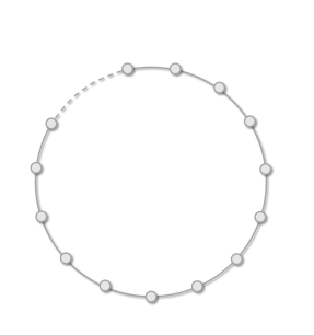
(a) ring network

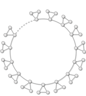
(b) triangle ring network

Figure 1: Illustrations of the ring network and the triangle ring network.

Recently, the reciprocal of the largest eigenvalue of the network’s non-backtracking matrix [15, 12] is introduced as a better theoretical estimate of the percolation threshold. We defer its technical definition to Section 2, and give an intuitive explanation on the issue of the adjacency matrix that is addressed by the non-backtracking matrix. Let $\pi$ be a vector, with $\pi_{i}$ representing the probability that node $i$ is in the giant connected component, when every edge has a probability of $p$ to be occupied. Let $A$ be the adjacency matrix of the graph, and ${\cal N}_{i}$ be the set of neighbors of $i$. The $i$-th entry of $pA\pi$ satisfies $[pA\pi]_{i}=\sum_{j\in{\cal N}_{i}}p\pi_{j}$, which approximately represents that $i$ could connect to the giant component through one of its neighbors $j$ (with probability $p\pi_{j}$). Thus it should be the same as $\pi_{i}$, and in matrix form, we have $pA\pi=\pi$. This suggests that $1/p$ should be at most $\lambda_{A}$, i.e. $1/\lambda_{A}$ is a lower bound of the percolation threshold. However, for every edge $(i,j)$ in the network, the above approximation considers both that $i$ may rely on $j$ to connect to the giant component and $j$ may rely on $i$, but the two cases should not jointly occur. Therefore, the estimate by $1/\lambda_{A}$ inflates the probability that a giant component emerges and underestimates the percolation threshold. The non-backtracking matrix addresses this issue by disallowing such directed circular dependency between a pair of nodes on an edge.

However, non-backtracking matrix only works well in locally treelike graphs. In non-treelike graphs, it provides a lower bound, bot not as close as the true percolation threshold. As suggested by the famous small-world network study [30], a significant amount of triangles exist in many real networks. The non-backtracking matrix does not eliminate the circular dependency through triangles or other local structures, and thus it may still underestimate the percolation threshold. For example, in the triangle ring network in Fig. 1b, the real percolation threshold is $1$, but the theoretical estimates by the adjacency and non-backtracking matrices are $0.3333$ and $0.5523$, respectively.

In this paper, we extend the idea of the non-backtracking matrix to define high-order non-backtracking matrices. We first define the high-order non-backtracking matrices and study the evolution of their largest eigenvalue with respect to order (Section 3). Then, we propose that the reciprocal of the largest eigenvalue of the 2nd-order non-backtracking matrix can provide a better estimate for the percolation threshold in an arbitrary network, because it eliminates the circular dependency from triangles (Section 3). We further provide an alternative matrix sharing the same largest eigenvalue but with substantially smaller size to improve computation efficiency. Finally, we conduct extensively experiments on both the forest fire model and 42 real networks to demonstrate the effectiveness of our method (Section 5).

To summarize, our contributions include: (i) proposing the high-order non-backtracking matrices and studying their eigenvalue properties; (ii) establishing a more precise theoretical estimation for bond percolation threshold and finding a faster approach to evaluate it; and (iii) supporting our analysis by empirical evaluations on synthetic and real networks.

1.1 Related Work

For random degree-uncorrelated network models, the percolation threshold can be approximated as $\langle d\rangle/(\langle d^{2}\rangle-\langle d\rangle)$ [9, 5]. Here, $\langle d\rangle$ and $\langle d^{2}\rangle$ are separately the first and the second moments of the degree distribution. This estimation is less predictive for real networks where degree correlations appear.

Bollobás et al. [3] show that the percolation threshold of dense graph is reciprocal of the largest eigenvalue of the adjacency matrix. However, the conclusion requires restrictive conditions for the networks. Especially for sparse networks, this estimation can be only regarded as providing a lower bound for the true percolation threshold.

Since a lot of realistic networks are sparse, Karrer et al. [15] and Hamilton et al. [12] simultaneously propose that the reciprocal of the largest eigenvalue of the non-backtracking matrix is a tighter lower bound for bond and site percolation threshold, respectively, on sparse networks. This prediction is based on a message passing technique and obtained by heuristic equations and approximations on locally treelike structures. Radicchi [25] further presents a mapping between the site and bond percolation to mathematically verify the predicted bond and site percolation thresholds are identical in this method. Although the estimation based on the non-backtracking matrix is more precise than that based on the adjacency matrix, it is still not close enough to the true percolation threshold on many real networks [26], since it suffers from the limitation of the treelike assumption. Radicchi et al. [27] also derives an alternative matrix of the non-backtracking matrix based on triangle elimination to improve the estimate for the site percolation threshold. However, this alternative matrix would overshoot on bond percolation. That means this estimate may overestimate the percolation threshold, leading it no longer provides a lower bound for the bond percolation threshold.

2 Preliminaries

We consider a finite connected undirected graph $\mathcal{G}=(\mathcal{V},\mathcal{E})$ with $N$ nodes and $E$ edges, where $\mathcal{V}=\{1,2,\cdots,N\}$ is the set of $N$ nodes and $\mathcal{E}=\{(i,j)\mid i,j\in\mathcal{V}\}$ is the set of $E$ edges. The connectivity between nodes in $\mathcal{G}$ is described by an adjacency matrix ${A}$, in which the element $a_{ij}=1$ if $(i,j)\in\mathcal{E}$, and $a_{ij}=0$ otherwise. We assume that $\cal G$ has no self-loops, i.e. $a_{ii}=0$ for all $i\in{\cal V}$. Henceforth, the adjacency and non-backtracking matrices are all refer to this graph $\cal G$, when the context is clear.

The bond percolation model is only controlled by one parameter, bond occupation probability $p$. That means, in a network $\mathcal{G}$, each edge is independently occupied with probability $p$. The percolation clusters are sets of nodes connected only by occupied edges. For $p=0$, no edge is occupied so that there are $N$ isolated clusters of size one. For $p=1$, all edges are occupied and all nodes compose a single cluster of size $N$. At intermediate values of $p$, the network undergoes two different phases: the non-percolating phase, where all clusters have microscopic size; the percolating phase, where a single macroscopic cluster (the giant component), whose size is comparable to the entire network, is present. The percolation threshold $p_{c}$ is the value above which the giant cluster appears; below $p_{c}$ there are only small clusters.

The transition can be monitored through two primary quantities of interest, the relative sizes of the first and second largest clusters with respect to the size of the network, denoted by $S_{1}(p)$ and $S_{2}(p)$, respectively. In order to evaluate percolation threshold numerically, there are many different estimates for $p_{c}$ being proposed, such as the occupation probability corresponding to the maximal value of $S_{2}(p)$, the peak position of the empirical variance of $S_{1}(p)$ and the average size of clusters except the largest one [26]. In this paper, we determine the best empirical estimate for percolation threshold as the value of $p$ where the second largest cluster reaches its maximum, namely

$$p_{c}=\arg\{\max_{p}S_{2}(p)\}.$$ (1)

In the following, we will compare it with theoretical approaches to check their validity.

The first theoretical estimate is based on the adjacency matrix. Bollobás et al. [3] show that for percolation on dense networks, the percolation threshold can be given by

$$p_{c}=\frac{1}{\lambda_{A}},$$

where $\lambda_{A}$ is the largest eigenvalue of matrix ${A}$, which is also the spectral radius of $A$. Although this estimate provides a good prediction for percolation threshold on networks with high density of connections, it becomes less precise on sparse networks.

Since a lot of realistic networks are sparse, a new estimate based on non-backtracking matrix [13, 17] is proposed to give a better prediction. For any undirected network $\mathcal{G}$, we can transform it to a directed one through replacing each undirected edge $(i,j)$ by two directed ones $i\to j$ and $j\to i$. The non-backtracking matrix, denoted by ${B}$, is a $2E\times 2E$ matrix with rows and columns indexed by directed edges $i\to j$ and entries are given by

$$B_{i\to j,k\to l}=\delta_{jk}(1-\delta_{il}),$$

where $\delta_{ij}$ is the Kronecker Delta Function ($\delta_{ij}=1$ if $i=j$, and $0$ if $i\neq j$). In other words, for any two directed edges $i\to j,j\to k$, $B_{i\to j,j\to k}=1$ if $k\neq i$, and thus $B_{i\to j,j\to k}$ records the walk from $i$ to $j$ and continuing to $k$ but not backtracking to $i$. Under the locally treelike assumption, which means that the local neighborhood of a node is close to a tree without redundant paths, the reciprocal of the largest eigenvalue of ${B}$ provides a close lower bound for sparse networks [15, 12], namely

$$p_{c}\geq\frac{1}{\lambda_{B}},\mbox{and }p_{c}\approx\frac{1}{\lambda_{B}}.$$

As already mentioned in the introduction, the non-backtracking matrix relies on the approximation of the locally treelike structure and it does not eliminate triangle dependency, and thus it may not give a tight lower bound of the bond percolation threshold. In the following, we propose a more powerful tool, high-order non-backtracking matrices, to better estimate bond percolation threshold.

3 High-Order Non-Backtracking
Matrices

In this section, we first introduce the definition of high-order non-backtracking matrices, and then investigate their properties.

In a network $\mathcal{G}$, let $i_{1}\to i_{2}\to\cdots\to i_{g+1}$ stand for a length-$g$ directed path composed by $g+1$ different nodes $i_{1},i_{2},\cdots,i_{g+1}$, obeying $a_{i_{k}i_{k+1}}=1$ ($1\leq k\leq g$). For the sake of saving space, we use $\overline{i_{1}i_{2}\cdots i_{g+1}}$ to stand for length-$g$ directed path in place of $i_{1}\to i_{2}\to\cdots\to i_{g+1}$. Let $P_{g}$ be the number of length-$g$ directed paths in $\mathcal{G}$. Then, we define the $g$-th-order non-backtracking matrix as follows:

Definition 1

The $g$-th-order non-backtracking matrix ${B}^{(g)}$ is a $P_{g}\times P_{g}$ matrix with rows and columns indexed by length-$g$ directed paths. The elements in ${B}^{(g)}$ are

$$B^{(g)}_{\overline{i_{1}i_{2}\cdots i_{g+1}},\overline{j_{1}j_{2}\cdots j_{g+1}}}=a_{i_{1}j_{1}}(1-\delta_{i_{1}j_{g+1}})\prod_{k=2}^{g+1}\delta_{i_{k}j_{k-1}}.$$ (2)

In other words, for each length-$(g+1)$ directed path, $\overline{i_{1}i_{2}\cdots i_{g+2}}$, we have $B^{(g)}_{\overline{i_{1}i_{2}\cdots i_{g+1}},\overline{i_{2}i_{3}\cdots i_{g+2}}}=1$; and all other entries of $B^{(g)}$ have value $0$. For example, if $\overline{123}$, $\overline{234}$, $\overline{345}$, and $\overline{231}$ are all length-$2$ directed paths in a graph, then ${B}^{(2)}_{\overline{123},\overline{234}}=1$, while ${B}^{(2)}_{\overline{123},\overline{345}}={B}^{(2)}_{\overline{123},\overline{231}}=0$. We can regard matrix ${B}^{(g)}$ as encoding the relations between length-$g$ directed paths in $\mathcal{G}$. It also describes a kind of non-backtracking walks with memory, avoiding going back to a node visited in the recent $g$ steps. It is easy to verify that the standard non-backtracking matrix is $B={B}^{(1)}$, and adjacency matrix $A={B}^{(0)}$ ($a_{i_{1}j_{1}}$ in Eq. (2) is explicitly for the case of $g=0$).

Let $\lambda_{B}^{(g)}$ be the largest eigenvalue of ${B}^{(g)}$. By the Perron-Frobenius Theorem [20], $\lambda_{B}^{(g)}$ is real and non-negative, and it is zero only when the directed graph with the adjacency matrix equal to ${B}^{(g)}$ is a directed acyclic graph (DAG). We now study the properties of $\lambda_{B}^{(g)}$ as $g$ changes. A simple cycle in graph $\mathcal{G}$ is a closed path with no repetitions of nodes and directed edges allowed, except the repetition of the starting and ending nodes. To maintain a consistent terminology, henceforth, all cycle means a simple cycle. The result is given in the following theorem:

Theorem 1

The $g$-th-order non-backtracking matrix ${B}^{(g)}$ satisfies the following properties:

(i) The largest eigenvalue of ${B}^{(g)}$ is non-increasing with respect to $g$, i.e., for every $g=1,2,3,\cdots$, $\lambda_{B}^{(g-1)}\geq\lambda_{B}^{(g)}$.

(ii) Let $\ell$ be the length of the longest simple cycle in graph $\mathcal{G}$. Then $\lambda_{B}^{(g)}=0$ for all $g\geq\ell-1$.

(iii) For any $\ell\geq 3$, if there is no simple cycle with length $\ell$ in $\cal G$, then $\lambda_{B}^{(\ell-2)}=\lambda_{B}^{(\ell-1)}$.

In order to prove Theorem 1, we first present some related notations and lemmata. The $g$-th-order non-backtracking matrix ${B}^{(g)}$ of network $\mathcal{G}$ can be regarded as the adjacency matrix of a directed network $\mathcal{G}^{(g)}=(\mathcal{V}^{(g)},\mathcal{E}^{(g)})$, where $\mathcal{V}^{(g)}=\{u\mid u$ is a length-$g$ directed path$\}$, and $\mathcal{E}^{(g)}=\{u\to v\mid u,v$ are two length-$g$ directed paths and $B^{(g)}_{u,v}=1\}$. Note that when $g=0$, $\mathcal{G}^{(0)}=\mathcal{G}$ (considering $\mathcal{G}$ as a symmetric directed graph). The line graph of $\mathcal{G}^{(g)}$ is $\bar{\mathcal{G}}^{(g)}=(\bar{\mathcal{V}}^{(g)},\bar{\mathcal{E}}^{(g)})$, where $\bar{\mathcal{V}}^{(g)}=\mathcal{E}^{(g)}$ and $\bar{\mathcal{E}}^{(g)}=\{\alpha\to\beta\mid\alpha=(u,v)$ and $\beta=(v,w)$ are two different edges $u\to v$ and $v\to w$ in $\mathcal{E}^{(g)}.\}$. Let $\bar{B}^{(g)}$ denote the adjacency matrix of the line graph $\bar{\mathcal{G}}^{(g)}$, with elements

$$\bar{B}^{(g)}_{u\to v,p\to q}=\delta_{vp},$$

where $u$, $v$, $p$ and $q$ are length-$g$ directed paths with $u\to v,p\to q\in{\cal E}^{(g)}$. In other words, we can recast definition of $\bar{B}^{(g)}$ as

$$\bar{B}^{(g)}_{\overline{i_{1}i_{2}\cdots i_{g+2}},\overline{j_{1}j_{2}\cdots j_{g+2}}}=\prod_{k=2}^{g+2}\delta_{i_{k}j_{k-1}}.$$

Lemma 1

$\mathcal{G}^{(g)}$ can be obtained by deleting all edges in all length-$(g+1)$ cycles in $\bar{\mathcal{G}}^{(g-1)}$.

Proof 3.2.

For each edge $u\to v$ ($u=\overline{i_{1}i_{2}\cdots i_{g}}$ and $v=\overline{i_{2}\cdots i_{g}i_{g+1}}$) in $\mathcal{G}^{(g-1)}$, it must correspond to a length-$g$ directed path $\overline{i_{1}\cdots i_{g}i_{g+1}}$ in $\mathcal{G}$. On the other hand, each length-$g$ directed path also corresponds to an edge in $\mathcal{G}^{(g-1)}$. Thus, $\mathcal{V}^{(g)}=\mathcal{E}^{(g-1)}=\bar{\mathcal{V}}^{(g-1)}$ if we identify $\overline{i_{1}i_{2}\cdots i_{g}}\to\overline{i_{2}\cdots i_{g}i_{g+1}}$ with $\overline{i_{1}\cdots i_{g}i_{g+1}}$, i.e., the node set of $\bar{\mathcal{G}}^{(g-1)}$ is identical to the node set of $\mathcal{G}^{(g)}$. Moreover, for every edge in $\mathcal{G}^{(g)}$, $\overline{i_{1}i_{2}\cdots i_{g+1}}\to\overline{i_{2}\cdots i_{g+1}i_{g+2}}{}$, it is also an edge in $\bar{\mathcal{G}}^{(g-1)}$, implying $\mathcal{E}^{(g)}\subseteq\bar{\mathcal{E}}^{(g-1)}$. For an arbitrary edge in $\bar{\mathcal{E}}^{(g-1)}\setminus\mathcal{E}^{(g)}$, it must have a form as $\overline{i_{1}i_{2}\cdots i_{g+1}}\to\overline{i_{2}\cdots i_{g+1}i_{1}}$, and there must be $g$ other edges with the same form together composing a length-$(g+1)$ cycle in $\bar{\mathcal{G}}^{(g-1)}$, namely $\overline{i_{1}i_{2}\cdots i_{g+1}}\to\overline{i_{2}\cdots i_{g+1}i_{1}}\to\cdots\to\overline{i_{g+1}i_{1}\cdots i_{g}}\to\overline{i_{1}i_{2}\cdots i_{g+1}}$. Moreover, for any length-$(g+1)$ cycle in $\bar{\mathcal{G}}^{(g-1)}$, it must be of the above form. If not, then it involves an edge of form $\overline{i_{1}i_{2}\cdots i_{g+1}}\to\overline{i_{2}\cdots i_{g+1}i_{g+2}}$ with $i_{g+2}\neq i_{1}$, the cycle must be of length at least $g+2$, because we have $g+2$ different original nodes $i_{1},\ldots,i_{g+2}$ in the cycle, and each edge in the cycle only removes one head node and adds one tail node, and thus it needs at least $g+2$ edges to go through every original node once and comes back to $\overline{i_{1}i_{2}\cdots i_{g+1}}$. Together, we know that by exactly removing all edges in all length-$(g+1)$ cycles in $\bar{\mathcal{G}}^{(g-1)}$, we obtain $\mathcal{G}^{(g)}$.

The next lemma is a known result saying that when we remove edges from a graph, the largest eigenvalue of the adjacency matrix will not increase.

Lemma 3.3 (Proposition 3.1.1 of [4]).

For the adjacency matrix $A$ of a graph $\mathcal{G}$, if $A^{\prime}$ is a matrix obtained by replacing some of the $1$’s in $A$ with $0$, then we have

$$\lambda_{A^{\prime}}\leq\lambda_{A},$$ (3)

where $\lambda_{A^{\prime}}$ and $\lambda_{A}$ are the largest eigenvalue of $A^{\prime}$ and $A$, respectively.

For convenience, we give an independent proof of Lemma 3.3 in Appendix LABEL:App1.

We are now ready to prove Theorem 1.

Proof 3.4 (of Theorem 1).

(i) For a directed graph $\mathcal{G}$ and its line graph, Pakoński et al. [24] show that their spectra excluding the possible eigenvalue zero are exactly the same. Therefore, we have

$$\lambda_{B}^{(g-1)}=\bar{\lambda}_{B}^{(g-1)},$$

where $\bar{\lambda}_{B}^{(g-1)}$ is the largest eigenvalue of matrix $\bar{B}^{(g-1)}$.

According to Lemma 1, $\mathcal{G}^{(g)}$ have the same node set as $\bar{\mathcal{G}}^{(g-1)}$, and $\mathcal{G}^{(g)}$ can be obtained by removing edges in length-$(g+1)$ cycles in $\bar{\mathcal{G}}^{(g-1)}$. Thus, applying Lemma 3.3, we attain the conclusion that

$$\lambda_{B}^{(g-1)}=\bar{\lambda}_{B}^{(g-1)}\geq\lambda_{B}^{(g)}.$$

(ii) We first claim that, $\mathcal{G}^{(g)}$ is a DAG for all $g\geq\ell-1$. If not, there are $k$ ($k\geq g+2$) length-$g$ directed paths in ${\cal G}^{(g)}$, $\overline{i_{1}i_{2}\cdots i_{g+1}}$, $\overline{i_{2}i_{3}\cdots i_{g+2}}$, …, $\overline{i_{k}i_{1}\cdots i_{g}}$, constituting a cycle in $\mathcal{G}^{(g)}$. Then there must be a length-$k$ cycle composed by $i_{1},i_{2},\cdots,i_{k}$ in $\mathcal{G}$. Since $g\geq\ell-1$, we have $k\geq\ell+1$, implying that there is at least one cycle in $\cal G$ with length larger than $\ell$, which contradicts to the assumption that the length of the largest cycle in $\mathcal{G}$ is $\ell$. Thus, network $\mathcal{G}^{(g)}$ is a DAG. It is easy to verify that the adjacency matrix of a DAG has the normal form where all block matrices on the diagonal are one-dimensional matrices with value $0$, and thus all its eigenvalues are $0$. Therefore $\lambda_{B}^{(g)}=0$ for all $g\geq\ell-1$.

(iii) Consider the line graph of ${\cal G}^{(\ell-2)}$, $\bar{\cal G}^{(\ell-2)}$. By Lemma 1, graph ${\cal G}^{(\ell-1)}$ is obtained by removing all length-$\ell$ cycles in $\bar{\cal G}^{(\ell-2)}$. Similar to the argument in the proof of Lemma 1, every length-$\ell$ cycle in $\bar{\cal G}^{(\ell-2)}$ has the form $\overline{i_{1}i_{2}\cdots i_{\ell}}$ $\to$ $\overline{i_{2}\cdots i_{\ell}i_{1}}\to$ $\cdots\overline{i_{\ell}i_{1}\cdots i_{\ell-1}}$ $\to\overline{i_{1}i_{2}\cdots i_{\ell}}$. Then every such cycle corresponds to a length-$\ell$ simple cycle in the original graph $\cal G$, $i_{1}\to i_{2}\to\cdots i_{\ell}\to i_{1}$. By assumption $\cal G$ has no length-$\ell$ simple cycles, thus it implies that $\bar{\cal G}^{(\ell-2)}$ is the same as ${\cal G}^{(\ell-1)}$. Since the line graph shares the same non-zero eigenvalues as the original graph [24], we know that $\lambda^{(\ell-1)}=\lambda^{(\ell-2)}$.

4 Estimating Percolation Threshold by 2nd-Order Non-Backtracking Matrix

In this section, we show that the reciprocal of the largest eigenvalue of the 2nd-order non-backtracking matrix gives a lower bound on the bond percolation threshold. According to Theorem 1, it implies that this lower bound is tighter than the previous proposed analytical lower bounds using the reciprocal of the adjacency matrix or the standard non-backtracking matrix. We then show that we can replace the 2nd-order non-backtracking matrix with a substantially smaller matrix sharing the same largest eigenvalue to improve computation efficiency.

4.1 Derivation of Lower Bound

Our derivation follows the message passing techniques proposed in [15, 12], which involves first-order analysis (ignoring higher-order terms) and heuristic equations on locally treelike graphs. Henceforth, we denote percolation threshold predicted by the adjacency matrix, non-backtracking matrix and 2nd-order non-backtracking matrix as $p_{c}^{(0)}$, $p_{c}^{(1)}$ and $p_{c}^{(2)}$, respectively.

Let $\pi_{i}$ be the probability that node $i$ belongs to the giant connected component, where the random events are that each edge in $\cal G$ is independently occupied with probability $p$. Let $\theta_{i\to j\to k}$ be the probability that node $i$ connects to the giant component following path $i\to j\to k$, where $i,j,k$ are all different nodes. Then, we can construct the following relation for bond percolation:

$$\pi_{i}=1-\prod_{\begin{subarray}{c}j\to k\\ j\in\mathcal{N}_{i},k\neq i\end{subarray}}(1-\theta_{i\to j\to k}),$$ (4)

Then, the expected size of the giant component can be given by

$$S_{1}(p)=\sum_{i=1}^{N}\pi_{i}.$$

In a finite-size network, there is a drastic change for $S_{1}(p)$ at the percolation threshold $p_{c}$. Next, we focus on predicting the value of $p_{c}$.

According to the definition of quantity $\theta_{i\to j\to k}$, we can construct recursive relations, which is appropriate for locally treelike structures with triangles:

$$\theta_{i\to j\to k}=1-\prod_{\ell\in\mathcal{N}_{k}\setminus\{i,j\}}(1-p\cdot\theta_{j\to k\to\ell}).$$ (5)

The above heuristic equation intuitively means that, node $i$ connects to the giant component through at least one of the paths $j\to k\to\ell$, and $i$ connects to $j$ with probability $p$ while $j$ connects to the giant component through path $j\to k\to\ell$ with probability $\theta_{j\to k\to\ell}$. The equation is approximately accurate when the local neighborhood of $i$ is close to a tree without redundant paths, except that we allow triangles such as $i\to j\to k\to i$, since the equation requires $\ell\neq i$, excluding such triangles. When we ignore $p^{2}$ and higher order terms in Eq. (5), we obtain

$$\theta_{i\to j\to k}=p\sum_{\ell\in\mathcal{N}_{k}\setminus\{i,j\}}\theta_{j\to k\to\ell},$$

which can be recast in matrix notation as

$$\theta=p{B}^{(2)}\theta,$$

where $\theta$ is a vector in which elements indexed by length-2 directed paths. When $p\geq p_{c}$, percolation happens, and $\theta$ should be a non-negative vector with some strictly positive entries. (It holds when length of the largest cycle is at least 4.) But if $p_{c}<1/\lambda^{(2)}_{B}$, it means we could have an eigenvalue of $1/p_{c}>\lambda^{(2)}_{B}$, violating the definition of $\lambda^{(2)}_{B}$. Therefore, we have

$$p_{c}\geq p_{c}^{(2)}=\frac{1}{\lambda^{(2)}_{B}}.$$

Theorem 1 theoretically guarantees $p_{c}^{(2)}\geq p_{c}^{(1)}\geq p_{c}^{(0)}$, so that $p_{c}^{(2)}$ provides a tighter lower bound for percolation threshold than the ones provided by the adjacency and standard non-backtracking matrices. Moreover, consider the example of triangle ring network shown in Figure 1b, it is easy to obtain $\lambda_{B}^{(2)}=1$ and $p_{c}^{(2)}=1/\lambda_{B}^{(2)}=1$, which is consistent with the true percolation threshold. Compared with estimates $p_{c}^{(0)}$ and $p_{c}^{(1)}$, $p_{c}^{(2)}$ exhibits remarkable improvement in precision.

The reason why $p_{c}^{(2)}$ provides better prediction of $p_{c}$ than $p_{c}^{(1)}$ can be heuristically explained as follows. In the estimation based on non-backtracking matrix, it only considers the probability node $i$ connects to the giant component through node $j$, which can be denoted as $\theta_{i\to j}$. If there is a triangle composed by nodes $i$, $j$ and $k$ in the network, $\theta_{i\to j}$ grows as $\theta_{j\to k}$ increases. Similarly, $\theta_{j\to k}$ increases with $\theta_{k\to i}$, and $\theta_{k\to i}$ increases with $\theta_{i\to j}$. This creates a triangular dependency which artificially inflates the values of $\theta_{i\to j}$, $\theta_{j\to k}$, and $\theta_{k\to i}$, leading to a higher estimate of the probability of giant component emergence and a lower estimate on the percolation threshold. When triangles are abundant, as evidenced by the small-world research on many real-world networks [30], using the standard non-backtracking matrix may still significantly underestimate the percolation threshold. By using the 2nd-order non-backtracking matrix, we avoid the triangular dependency, so that $p_{c}^{(2)}$ is more precise than $p_{c}^{(1)}$.

Although $p_{c}^{(2)}$ is a tighter lower bound, the size of ${B}^{(2)}$ is usually larger than ${B}$, leading to higher computation complexity. In the following we provide a further technique to tackle this problem.

4.2 Improving Computation Efficiency

In this subsection, we illustrate that we can transfer the task of computing eigenvalues of ${B}^{(2)}$ to calculating eigenvalues of a new matrix ${M}$, defined as

$${M}=\left(\begin{array}[]{cccc}{B}^{(1)}&-\Delta{B}_{2}&{D}_{\Delta}-{I}&{B}^{(1)}-\Delta{B}_{1}\\ {I}&{0}&{0}&{0}\\ {0}&{I}&{0}&{0}\\ {0}&{0}&{I}&{0}\end{array}\right).$$ (10)

Here, ${M}$ is a square matrix of dimension $8E\times 8E$ composed of $16$ $2E\times 2E$ blocks, whose size is evidently smaller than ${B}^{(2)}$. Matrix $\Delta{B}_{1}$ and $\Delta{B}_{2}$ have identical size with ${B}^{(1)}$ and their elements are defined as

$$(\Delta B_{1})_{i\to j,k\to\ell}=\left\{\begin{aligned} &1,\quad a_{i\ell}B^{(1)}_{i\to j,k\to\ell}=1,\\ &0,\quad{\rm otherwise.}\end{aligned}\right.$$

and

$$(\Delta B_{2})_{i\to j,k\to\ell}=\left\{\begin{aligned} &1,\quad\delta_{i\ell}a_{ij}a_{jk}a_{k\ell}=1,\\ &0,\quad{\rm otherwise,}\end{aligned}\right.$$

respectively. The matrix ${D}_{\Delta}$ is a $2E\times 2E$ diagonal matrix and its element $(D_{\Delta})_{i\to j,i\to j}$ equals the number of triangles containing edge $(i,j)$.

Theorem 4.5.

The set of non-zero eigenvalues of matrix $M$ defined in Eq. (10) consists of all non-zero eigenvalues of the 2nd-order non-backtracking matrix ${B}^{(2)}$ and possibly eigenvalues $-1$, $(1+\sqrt{3}\mathrm{i})/2$ and $(1-\sqrt{3}\mathrm{i})/2$.

Proof 4.6.

The proof will include two parts. First, we prove that every non-zero eigenvalue of $B^{(2)}$ corresponds to an eigenvalue of $M$. Second, we elaborate that every non-zero eigenvalue of $M$ equals to one of eigenvalues of $B^{(2)}$, except possible eigenvalues $-1$, $(1+\sqrt{3}\mathrm{i})/2$ and $(1-\sqrt{3}\mathrm{i})/2$.

(i) Let $\lambda$ be an arbitrary non-zero eigenvalue of ${B}^{(2)}$ and $\psi$ be its corresponding eigenvector. According to the definition of the 2nd-order non-backtracking matrix, we have

$$\lambda\psi_{i\to j\to k}=\sum_{\ell\in\mathcal{N}_{k}\setminus\{i,j\}}B^{(1)}_{j\to k,k\to l}\psi_{j\to k\to\ell}.$$ (11)

In order to show each non-zero eigenvalue of $B^{(2)}$ is also an eigenvalue of $M$, we first introduce two related quantities:

$$x_{i\to j}=\sum_{k\in\mathcal{N}_{j}\setminus\{i\}}B^{(1)}_{i\to j,j\to k}\psi_{i\to j\to k}$$ (12)

and

$$y_{i\to j}=\sum_{k\in\mathcal{N}_{j}\setminus\{i\}}B^{(1)}_{i\to j,j\to k}B^{(1)}_{j\to k,k\to i}\psi_{i\to j\to k}.$$ (13)

Let $x$ and $y$ be vectors with elements $x_{i\to j}$ and $y_{i\to j}$, respectively. We claim that $x$ and $y$ satisfies the following two relations:

$$x=\frac{1}{\lambda}{B}^{(1)}x-\frac{1}{\lambda^{2}}\Delta{B}_{2}x+\frac{1}{\lambda^{3}}{D}_{\Delta}x-\frac{1}{\lambda^{3}}y$$ (14)

and

$$y=\frac{1}{\lambda}\Delta{B}_{1}x-\frac{1}{\lambda^{2}}\Delta{B}_{2}x+\frac{1}{\lambda^{3}}{D}_{\Delta}x-\frac{1}{\lambda^{3}}y,$$ (15)

which will be proved latter.

Combining Eq. (14) and Eq. (15), we can obtain

$$x-y=\frac{1}{\lambda}({B}^{(1)}-\Delta{B}_{1})x,$$

which indicates

$$y=\left({I}-\frac{1}{\lambda}{B}^{(1)}+\frac{1}{\lambda}\Delta{B}_{1}\right)x.$$ (16)

Plugging Eq. (16) into Eq. (14) yields

$$x = \frac{1}{\lambda}{B}^{(1)}x-\frac{1}{\lambda^{2}}\Delta{B}_{2}x+\frac{1}{\lambda^{3}}\left({D}_{\Delta}-{I}\right)x$$ (17)

$$+\frac{1}{\lambda^{4}}({B}^{(1)}-\Delta{B}_{1})x.$$

Based on Eq. (17), we establish

$${M}z=\lambda z,$$

where $z=(x^{\top},\frac{1}{\lambda}x^{\top},\frac{1}{\lambda^{2}}x^{\top},\frac{1}{\lambda^{3}}x^{\top})^{\top}$. Thus, every non-zero eigenvalue of $B^{(2)}$ corresponds to an eigenvalue of $M$.

Proof of Eq. (14). Plugging Eq. (11) into Eq. (12), we have

$$x_{i\to j} = \frac{1}{\lambda}\sum_{k\in\mathcal{N}_{j}\setminus\{i\}}B^{(1)}_{i\to j,j\to k}\sum_{\ell\in\mathcal{N}_{k}\setminus\{j\}}B^{(1)}_{j\to k,k\to\ell}\psi_{j\to k\to\ell}$$ (18)

$$-\frac{1}{\lambda}\sum_{k\in\mathcal{N}_{j}\cap\mathcal{N}_{i}}B^{(1)}_{i\to j,j\to k}B^{(1)}_{j\to k,k\to i}\psi_{j\to k\to i}.$$

In the r.h.s of Eq. (18), the first term can be rewritten as

$$\frac{1}{\lambda}\sum_{k\in\mathcal{N}_{j}\setminus\{i\}}B^{(1)}_{i\to j,j\to k}\sum_{\ell\in\mathcal{N}_{k}\setminus\{j\}}B^{(1)}_{j\to k,k\to\ell}\psi_{j\to k\to\ell}$$ (19)

$$= \frac{1}{\lambda}\sum_{k\in\mathcal{N}_{j}\setminus\{i\}}B^{(1)}_{i\to j,j\to k}x_{j\to k}.$$

Here, Eq. (12) is used. Utilizing Eq. (11) again, the second term of r.h.s of Eq. (18) can be represented as

$$\frac{1}{\lambda}\sum_{k\in\mathcal{N}_{j}\cap\mathcal{N}_{i}}B^{(1)}_{i\to j,j\to k}B^{(1)}_{j\to k,k\to i}\psi_{j\to k\to i}$$ (20)

$$= \frac{1}{\lambda^{2}}\sum_{k\in\mathcal{N}_{j}\cap\mathcal{N}_{i}}B^{(1)}_{i\to j,j\to k}B^{(1)}_{j\to k,k\to i}\sum_{\ell\in\mathcal{N}_{i}\setminus\{k\}}B^{(1)}_{k\to i,i\to\ell}\psi_{k\to i\to\ell}$$

$$-\frac{1}{\lambda^{2}}\sum_{k\in\mathcal{N}_{j}\cap\mathcal{N}_{i}}B^{(1)}_{i\to j,j\to k}B^{(1)}_{j\to k,k\to i}B^{(1)}_{k\to i,i\to j}\psi_{k\to i\to j}$$

$$= \frac{1}{\lambda^{2}}\sum_{k\in\mathcal{N}_{j}\cap\mathcal{N}_{i}}B^{(1)}_{i\to j,j\to k}B^{(1)}_{j\to k,k\to i}x_{k\to i}$$

$$-\frac{1}{\lambda^{3}}\sum_{k\in\mathcal{N}_{j}\cap\mathcal{N}_{i}}B^{(1)}_{i\to j,j\to k}B^{(1)}_{j\to k,k\to i}\sum_{\ell\in\mathcal{N}_{j}\setminus\{i\}}B^{(1)}_{i\to j,j\to\ell}\psi_{i\to j\to\ell}$$

$$+\frac{1}{\lambda^{3}}\sum_{k\in\mathcal{N}_{j}\cap\mathcal{N}_{i}}B^{(1)}_{i\to j,j\to k}B^{(1)}_{j\to k,k\to i}\psi_{i\to j\to k}$$

$$= \frac{1}{\lambda^{2}}\sum_{k\in\mathcal{N}_{j}\cap\mathcal{N}_{i}}B^{(1)}_{i\to j,j\to k}B^{(1)}_{j\to k,k\to i}x_{k\to i}$$

$$-\frac{\Delta_{i\to j}}{\lambda^{3}}x_{i\to j}+\frac{1}{\lambda^{3}}y_{i\to j},$$

where $\Delta_{i\to j}$ is the number of length-3 loops starting from edge $i\to j$.

Inserting Eq. (19) and Eq. (20) into Eq. (18), we have

$$x_{i\to j} = \frac{1}{\lambda}\sum_{k\in\mathcal{N}_{j}\setminus\{i\}}B^{(1)}_{i\to j,j\to k}x_{j\to k}$$

$$-\frac{1}{\lambda^{2}}\sum_{k\in\mathcal{N}_{j}\cap\mathcal{N}_{i}}B^{(1)}_{i\to j,j\to k}B^{(1)}_{j\to k,k\to i}x_{k\to i}$$

$$+\frac{\Delta_{i\to j}}{\lambda^{3}}x_{i\to j}-\frac{1}{\lambda^{3}}y_{i\to j}.$$

Recasting Eq. (4.6) in matrix notation, we can obtain Eq. (14).

Proof of Eq. (15). Analogously, substituting Eq. (11) into Eq. (13), $y_{i\to j}$ can be represented as

$$y_{i\to j} = \frac{1}{\lambda}\sum_{k\in\mathcal{N}_{j}\setminus\{i\}}B^{(1)}_{i\to j,j\to k}B^{(1)}_{j\to k,k\to i}$$ (21)

$$\sum_{\ell\in\mathcal{N}_{k}\setminus\{j\}}B^{(1)}_{j\to k,k\to\ell}\psi_{j\to k\to\ell}$$

$$-\frac{1}{\lambda}\sum_{k\in\mathcal{N}_{j}\setminus\{i\}}B^{(1)}_{i\to j,j\to k}B^{(1)}_{j\to k,k\to i}\psi_{j\to k\to i}.$$

The first term in r.h.s of Eq. (21) can be further expressed as

$$\frac{1}{\lambda}\sum_{k\in\mathcal{N}_{j}\setminus\{i\}}B^{(1)}_{i\to j,j\to k}B^{(1)}_{j\to k,k\to i}\sum_{\ell\in\mathcal{N}_{k}\setminus\{j\}}B^{(1)}_{j\to k,k\to\ell}\psi_{j\to k\to\ell}$$ (22)

$$= \frac{1}{\lambda}\sum_{k\in\mathcal{N}_{j}\setminus\{i\}}B^{(1)}_{i\to j,j\to k}B^{(1)}_{j\to k,k\to i}x_{j\to k}.$$

Instituting Eq. (20) and Eq. (22) into Eq. (21), one has

$$y_{i\to j} = \frac{1}{\lambda}\sum_{k\in\mathcal{N}_{j}\setminus\{i\}}B^{(1)}_{i\to j,j\to k}B^{(1)}_{j\to k,k\to i}x_{j\to k}$$

$$-\frac{1}{\lambda^{2}}\sum_{k\in\mathcal{N}_{j}\setminus\{i\}}B^{(1)}_{i\to j,j\to k}B^{(1)}_{j\to k,k\to i}x_{k\to i}$$

$$+\frac{\Delta_{i\to j}}{\lambda^{3}}x_{i\to j}-\frac{1}{\lambda^{3}}y_{i\to j},$$

which can be recast in matrix form to obtain Eq. (15).

(ii) Now, we prove that every non-zero eigenvalue of $M$ equals to one of eigenvalues of $B^{(2)}$, except possible eigenvalues $-1$, $(1+\sqrt{3}\mathrm{i})/2$ and $(1-\sqrt{3}\mathrm{i})/2$. Let $\lambda$ be an arbitrary non-zero eigenvalue of $M$ and $z=(x^{\top},\frac{1}{\lambda}x^{\top},\frac{1}{\lambda^{2}}x^{\top},\frac{1}{\lambda^{3}}x^{\top})^{\top}$ be its corresponding eigenvector. According to Eq. (11) and Eq. (12), we have

$$\lambda\psi_{i\to j\to k}=\left\{\begin{aligned} &x_{j\to k}-\psi_{j\to k\to i},i\in\mathcal{N}_{k}\\ &x_{j\to k},i\notin\mathcal{N}_{k}.\end{aligned}\right.$$ (23)

Thus, for the case of nodes $i$, $j$ and $k$ constituting a triangle, we can establish the following equations:

$$\left\{\begin{aligned} &\lambda\psi_{i\to j\to k}+\psi_{j\to k\to i}=x_{j\to k}\\ &\lambda\psi_{j\to k\to i}+\psi_{k\to i\to j}=x_{k\to i}\\ &\lambda\psi_{k\to i\to j}+\psi_{i\to j\to k}=x_{i\to j}\end{aligned}\right..$$

When $\lambda^{3}+1\neq 0$, i.e. $\lambda\neq-1,(1+\sqrt{3}\mathrm{i})/2$ or $(1-\sqrt{3}\mathrm{i})/2$, we have solutions as

$$\left\{\begin{aligned} &\psi_{i\to j\to k}=\frac{1}{\lambda^{3}+1}(\lambda^{2}x_{j\to k}-\lambda x_{k\to i}+x_{i\to j})\\ &\psi_{j\to k\to i}=\frac{1}{\lambda^{3}+1}(\lambda^{2}x_{k\to i}-\lambda x_{i\to j}+x_{j\to k})\\ &\psi_{k\to i\to j}=\frac{1}{\lambda^{3}+1}(\lambda^{2}x_{i\to j}-\lambda x_{j\to k}+x_{k\to i})\end{aligned}\right..$$ (24)

Combining Eq. (23) and Eq. (24), we have

$$\psi_{i\to j\to k}=\left\{\begin{aligned} &\frac{1}{\lambda^{3}+1}(\lambda^{2}x_{j\to k}-\lambda x_{k\to i}+x_{i\to j}),i\in\mathcal{N}_{k}\\ &\frac{1}{\lambda}x_{j\to k},i\notin\mathcal{N}_{k}\end{aligned}\right..$$ (25)

Thus, for any non-zero eigenvalue $\lambda$ of $M$ except $-1$, $(1+\sqrt{3}\mathrm{i})/2$ and $(1-\sqrt{3}\mathrm{i})/2$, it satisfies $B^{(2)}\psi=\lambda\psi$, and the values of elements in $\psi$ can be determined by Eq. (25).

Exploiting Theorem 4.5, we give an approach to save time and space cost for computing $p_{c}^{(2)}$. In particular, the numbers of edges and length-2 directed paths in a network $\mathcal{G}$ are $E=\frac{1}{2}\sum_{i=1}^{N}d_{i}$ and $P_{2}=\sum_{i=1}^{N}d_{i}(d_{i}-1)$, respectively, where $d_{i}$ is the degree of node $i$. Thus, we reduce the size of the matrix to be computed by a factor of $(\sum_{i=1}^{N}d_{i}^{2}-\sum_{i=1}^{N}d_{i})/(4\sum_{i=1}^{N}d_{i})\approx\langle d^{2}\rangle/(4\langle d\rangle)$.

5 Experiments

In this section, we empirically investigate the validity of our theoretical estimate for bond percolation threshold. First, we compare $p_{c}^{(2)}$ with other theoretical indicators $p_{c}^{(1)}$ and $p_{c}^{(0)}$ on a class of synthetic networks generated by the forest fire model [19]. Next, we perform extensive experiments on 42 real networks to further explore the performance of these estimations.

We use the peak value of the second largest component (Eq. (1)) as the ground truth of the bond percolation threshold $p_{c}$. For each network, the value of the empirical ground truth $p_{c}$ is computed by 1000 independent Monte Carlo simulations of the percolation process as proposed by Newman and Ziff [22].

(a) burning probability $0.01$

(b) 5000 nodes

Figure 2: Empirical and theoretical estimates of the percolation threshold on the forest fire model.

(a) scatter plot

(b) cumulative distribution of relative errors

Figure 3: Test results of empirical and theoretical percolation thresholds on 42 real-world networks.

(a) relative errors vs. empirical estimates

(b) relative errors vs. average degrees

(c) relative errors vs. categories

Figure 4: Relative errors of theoretical percolation thresholds on 42 real-world networks.

5.1 Forest Fire Model

The forest fire model [19] is a family of evolutionary networks, controlled by burning probability $q$.

We denote the network at time $t$ as $G_{t}$. Initially ($t=1$), there is only one node in $G_{1}$. At time $t>1$, there is a new node $u$ joining the network $G_{t-1}$ and generating $G_{t}$. The node $u$ establishes connections with other existing nodes through the following process: (1) Node $u$ first selects an ambassador node $v$ in $G_{t-1}$ uniformly at random and connects to it. (2) We sample a random number $a\in(0,1]$. If $a\leq q$, node $u$ randomly chooses a neighbor of $v$, which is not connected to $u$ yet, and forms a link to it. Then repeat this step. If $a>q$, this step ends and we label all nodes linking to $u$ at this step as $w_{1},w_{2},\cdots,w_{k}$; (3) Let $w_{1},w_{2},\cdots,w_{k}$ sequentially be the ambassador of node $u$ and apply step (2) for each of them recursively. A node in the process should not be visited a second time.

The generation process of the forest fire model describes new nodes joining social networks with an epidemic fashion. In addition, forest fire model shares a number of remarkable structural features with real networks, such as densification and shrinking diameters [19]. Thus, studying percolation on the forest fire model can enhance our understanding of spreading in realistic systems.

We first consider a case that the burning probability is very small, so that the network $G_{t}$ is sparse. In Figure 2a, we plot bond percolation threshold estimated by different approaches during the evolution of a forest fire model with $q=0.01$. It shows that along with the growth of the network, the empirical estimate tends to $0.901$. The predicted percolation thresholds based on the adjacency and non-backtracking matrices tend to $0.210$ and $0.495$, respectively, which are far from the empirical estimate. Although $p_{c}^{(1)}$ performs better than $p_{c}^{(0)}$ in sparse networks, the appearance of triangle structures largely weakens its effectiveness. The estimation based on the 2nd-order non-backtracking matrix shows remarkable improvement. At the end of the evolution, $p_{c}^{(2)}$ tends to $0.778$, which corresponds to an improvement of roughly $30\%$ from $p_{c}^{(1)}$. It indicates $p_{c}^{(2)}$ is evidently more precise than $p_{c}^{(1)}$ for sparse networks with triangles.

Next we test the impact of burning probability on our indicator. In Figure 2b, we show the percolation threshold given by the theoretical and simulated estimations versus burning probability on forest fire model with 5000 nodes. Each value is the average of 100 networks. We observe that, along with the growth of the burning probability, the empirical percolation threshold decreases, because of the increase of the number of edges. For the theoretical indicators, it is not surprising that $p_{c}^{(2)}$ always performs better than $p_{c}^{(1)}$ and $p_{c}^{(0)}$, especially in the regime of small burning probability. However, as burning probability becomes large, the precision of $p_{c}^{(2)}$ decreases. In addition, the values of $p_{c}^{(0)}$,$p_{c}^{(1)}$ and $p_{c}^{(2)}$ are getting close. This is because the growth of the burning probability introduces more and more simple cycles with length larger than 3, which would lead to overestimating probability $\theta_{i\to j\to k}$ for $i\to j\to k$ in such a cycle. Thus, $p_{c}^{(2)}$ becomes less effective in predicting the percolation threshold.

5.2 Real Networks

For the purpose of better understanding the predictive power of different theoretical estimations in real networks, we evaluate bond percolation threshold predicted by $p_{c}^{(0)}$, $p_{c}^{(1)}$, $p_{c}^{(2)}$ and simulations on 42 real networks. The dataset includes social, infrastructural, animal and biological networks, which exhibit various topological properties, with size from 23 to 4941. In Table 1, we report the theoretical and empirical estimations for bond percolation threshold on the 42 real networks. All networks are treated as undirected unweighted networks. We only consider the largest connected component in each network. All datasets are from the Koblenz Network Collection (http://konect.uni-koblenz.de/).

In Appendix LABEL:App2, we display the structural information and detailed results for each network.

Figure 3a reports values of $p_{c}^{(0)}$, $p_{c}^{(1)}$ and $p_{c}^{(2)}$ as functions of the empirical estimate for all 42 networks. It shows that $p_{c}^{(2)}$ is always closer to the empirical estimate than $p_{c}^{(1)}$ and $p_{c}^{(0)}$, which is in agreement with our theoretical analysis. In addition, we observe that there are some networks on which $p_{c}^{(2)}$ can attain the empirical estimate. However, $p_{c}^{(2)}$ is not always close enough to the empirical estimate, especially on networks in the regime of large percolation threshold.

Next, we continue to quantitatively analyze how much improvement our proposed method attains. We define relative error of the theoretical estimate as $(p_{c}-p_{c}^{(\alpha)})/p_{c}$ ($\alpha=0,1$ or $2$). Then, we plot cumulative distribution of relative errors of $p_{c}^{(2)}$, $p_{c}^{(1)}$ and $p_{c}^{(0)}$ in the collection of 42 networks, as shown in Figure 3b. We adopt the area under the curve (AUC) as a measurement for global performance. The results is that there is an improvement of 8% from $p_{c}^{(0)}$ to $p_{c}^{(1)}$, and 3% from $p_{c}^{(1)}$ to $p_{c}^{(2)}$.

In order to further understand the influence of the true percolation threshold on our theoretical prediction, we first divide the range of possible values of the empirical estimate in eight bins. Then, we calculate the average of the empirical estimate and relative errors, respectively, in each bin. Figure 4a reports the average of relative error with respect to the average of the empirical estimate. It implies that $p_{c}^{(2)}$ works well on the networks in the range of small true percolation threshold; while it become less predictive on networks with large true percolation threshold.

We also analyze the impact of density of networks on our theoretical prediction. Analogously, we divide the range of possible values of average degree in seven bins and separately calculate the means of average degree and relative errors in each bin. In Figure 4b, we plot the relative error as a function of average degree for all three theoretical estimates. There are two main conclusions from this figure. First, for all three theoretical predictions, they are more precise on networks with large average degree than on networks with small average degree. Second, on networks in the regime of small average degree, $p_{c}^{(2)}$ in general has a better improvement from $p_{c}^{(1)}$ than on networks with relatively large average degree. It can be accounted as on dense networks, $p_{c}^{(0)}$ is already a good approximation for percolation threshold, and under such case $p_{c}^{(0)}$, $p_{c}^{(1)}$ and $p_{c}^{(2)}$ would be very close to each other.

At last, we discover the performance of theoretical predictions in different categories of networks. In Figure 4c, we give the average of relative errors in each group of networks for all three theoretical estimations. It can be found that theoretical predictions are closer to true percolation threshold in animal and social networks than in infrastructural and biological networks.

Network	Nodes	Edges	$p_{c}^{(0)}$	$p_{c}^{(1)}$	$p_{c}^{(2)}$	$p_{c}$
Animal Networks
Zebra	23	105	0.0814	0.0889	0.0969	0.1146
Bison	26	222	0.0544	0.0577	0.0608	0.0651
Cattle	28	160	0.0729	0.0796	0.0847	0.0875
Sheep	28	235	0.0548	0.0581	0.0609	0.0656
Dolphins	62	159	0.1390	0.1668	0.1791	0.2717
Macaques	62	1167	0.0256	0.0263	0.0268	0.0308
Social Networks
Seventh Graders	29	250	0.0532	0.0564	0.0592	0.0633
Dutch College	32	422	0.0367	0.0381	0.0395	0.0432
Zachary Karate Club	34	78	0.1487	0.1889	0.2097	0.2310
Windsurfers	43	336	0.0552	0.0588	0.0614	0.0712
Train bombing	64	243	0.0739	0.0815	0.0878	0.1330
Hypertext 2009	113	2196	0.0214	0.0219	0.0222	0.0262
Physicians	117	465	0.0994	0.1138	0.1176	0.1421
Manufacturing Emails	167	3250	0.0165	0.0168	0.0171	0.0200
Jazz Musicians	198	2742	0.0250	0.0258	0.0263	0.0335
Residence Hall	217	1839	0.0464	0.0492	0.0503	0.0629
Haggle	274	2124	0.0193	0.0198	0.0202	0.0246
Network Science	379	914	0.0964	0.1148	0.1294	0.3862
Infectious	410	2765	0.0428	0.0450	0.0465	0.0807
Crime	829	1473	0.1565	0.2198	0.2220	0.2628
Email	1133	5451	0.0482	0.0519	0.0529	0.0642
Hamsterster Friendships	1788	12476	0.0217	0.0226	0.0228	0.0266
Hamsterster Full	2000	16098	0.0200	0.0207	0.0210	0.0258
Facebook	2888	2981	0.0360	0.1339	0.1456	0.2885
Infrastructural Networks
Contiguous USA	49	107	0.1880	0.2400	0.2723	0.3610
Euroroad	1039	1305	0.2493	0.3906	0.4050	0.5908
Air Traffic	1226	2408	0.1086	0.1336	0.1387	0.2022
Open Flights	2905	15645	0.0159	0.0163	0.0165	0.0193
US Power	4941	6594	0.1336	0.1606	0.1766	0.6518
Biological Networks
PDZBase	161	209	0.1712	0.2483	0.2484	0.5237
Caenorhabditis Elegans	453	2025	0.0380	0.0426	0.0442	0.0533
Protein	1458	1948	0.1327	0.1980	0.2154	0.3094
Human Protein	1615	3106	0.0571	0.0648	0.0649	0.0876
Protein Figeys	2217	6418	0.0317	0.0359	0.0360	0.0474
Protein Vidal	2783	6007	0.0628	0.0761	0.0770	0.0975
Other Networks
Corporate Leadership	24	86	0.1167	0.1339	0.1430	0.1512
Florida Ecosystem Dry	128	2106	0.0249	0.0257	0.0260	0.0308
Florida ecosystem Wet	128	2075	0.0252	0.0260	0.0264	0.0315
Little Rock Lake	183	2434	0.0242	0.0250	0.0253	0.0313
Unicode Languages	614	1245	0.0637	0.0811	0.0853	0.1059
Blogs	1222	16714	0.0135	0.0138	0.0139	0.0167
Bible	1773	7105	0.0198	0.0247	0.0257	0.0268

Table 1: Percolation threshold for 42 real networks.

6 Discussion and Future Work

Figure 5: Bond percolation on a Barabási-Albert network with 50 nodes and mean degree 4. The empirical estimate is $p_{c}=0.2834$.

Although $p_{c}^{(2)}$ outperforms other theoretical estimations for bond percolation threshold, it is still not sufficiently precise on some real networks, due to the appearance of cycles larger than 3. A direct idea to further improve the precision is to use the reciprocal of the largest eigenvalue of higher order non-backtracking matrices as the predictor for the percolation threshold. According to a similar deduction as in Section 4.1, applying a $g$-th-order non-backtracking matrix should avoid overestimating probability that node $i$ connecting to the giant component following a length-$g$ path. Moreover, Theorem 1 also theoretically guarantees percolation threshold estimated by $g$-th-order non-backtracking matrix is non-decreasing with respect to $g$. In order to elaborate it empirically, we consider bond percolation on a small network with only 50 nodes, generated by the Barabási-Albert network model [2]. In Figure 5, we give the expected relative sizes of the first and second largest cluster as a function of probability $p$. In addition, we derive theoretical estimations for percolation threshold based on $g$-th-order non-backtracking matrix ($0\leq g\leq 5$), denoted separately as $p_{c}^{(g)}$. We can observe $p_{c}^{(3)}$ is a better approximation than $p_{c}^{(2)}$.

However, theoretical estimation based on high-order non-backtracking matrices still suffers the following two drawbacks. First, along with the increase of $g$, the size of the $g$-th-order non-backtracking matrix grows dramatically. It would lead to a prohibitive cost for computing the largest eigenvalue for large-scale networks. Second, with a sufficiently large $g$, $p_{c}^{(g)}$ could be larger than the true percolation threshold. As shown in Figure 5, $p_{c}^{(4)}$ and $p_{c}^{(5)}$ are already slightly larger than the peak position of $S_{2}(p)$. It may be because the heuristic analysis in Section 4.1 will be no longer hold for high-order non-backtracking matrices. Thus, possible directions of future work include finding efficient techniques for generating and analyzing high-order non-backtracking matrices, and determining at which order $p_{c}^{(g)}$ is the closest to but still smaller than the true percolation threshold. It is also possible that we can depart from non-backtracking matrices and use some brand-new techniques to develop the theoretical assessment of the percolation threshold.

In addition, the current lower bound derivation is based on heuristic equations. A more mathematically sound technique to show the effectiveness of high-order non-backtracking matrices and the exact conditions that support this effectiveness is also a future direction.

7 Acknowledgments

The authors thank anonymous reviewers for their valuable comments and helpful suggestions. Yuan Lin and Zhongzhi Zhang are supported by the National Natural Science Foundation of China (Grant No. 11275049). Wei Chen is partially supported by the National Natural Science Foundation of China (Grant No. 61433014).

References

- [1] J. Andrews, S. Shakkottai, R. Heath, N. Jindal, M. Haenggi, R. Berry, D. Guo, M. Neely, S. Weber, S. Jafar, and A. Yener. Rethinking information theory for mobile ad hoc networks. IEEE Communications Magazine, 46(12):94–101, 2008.
- [2] A.-L. Barabási and R. Albert. Emergence of scaling in random networks. Science, 286(5439):509–512, 1999.
- [3] B. Bollobás, C. Borgs, J. Chayes, and O. Riordan. Percolation on dense graph sequences. The Annals of Probability, 38(1):150–183, 2010.
- [4] A. E. Brouwer and W. H. Haemers. Spectra of graphs. Springer Science & Business Media, 2011.
- [5] D. S. Callaway, M. E. Newman, S. H. Strogatz, and D. J. Watts. Network robustness and fragility: Percolation on random graphs. Physical Review Letters, 85(25):5468, 2000.
- [6] C. Chen, H. Tong, B. A. Prakash, T. Eliassi-Rad, M. Faloutsos, and C. Faloutsos. Eigen-optimization on large graphs by edge manipulation. ACM Transactions on Knowledge Discovery from Data, 10(4):49, 2016.
- [7] C. Chen, H. Tong, B. A. Prakash, C. E. Tsourakakis, T. Eliassi-Rad, C. Faloutsos, and D. H. Chau. Node immunization on large graphs: Theory and algorithms. IEEE Transactions on Knowledge and Data Engineering, 28(1):113–126, 2016.
- [8] P.-Y. Chen, S.-M. Cheng, and K.-C. Chen. Smart attacks in smart grid communication networks. IEEE Communications Magazine, 50(8):24–29, 2012.
- [9] R. Cohen, K. Erez, D. Ben-Avraham, and S. Havlin. Resilience of the internet to random breakdowns. Physical Review Letters, 85(21):4626, 2000.
- [10] M. Franceschetti, O. Dousse, N. David, and P. Thiran. Closing the gap in the capacity of wireless networks via percolation theory. IEEE Transactions on Information Theory, 53(3):1009–1018, 2007.
- [11] S. Galli, A. Scaglione, and Z. Wang. For the grid and through the grid: The role of power line communications in the smart grid. Proceedings of the IEEE, 99(6):998–1027, 2011.
- [12] K. E. Hamilton and L. P. Pryadko. Tight lower bound for percolation threshold on an infinite graph. Physical Review Letters, 113(20):208701, 2014.
- [13] K. Hashimoto. Zeta functions of finite graphs and representations of p-adic groups. Advanced Studies in Pure Mathematics, 15:211–280, 1989.
- [14] L. Jiang, Y. Miao, Y. Yang, Z. Lan, and A. G. Hauptmann. Viral video style: a closer look at viral videos on youtube. In Proceedings of International Conference on Multimedia Retrieval, page 193. ACM, 2014.
- [15] B. Karrer, M. E. Newman, and L. Zdeborová. Percolation on sparse networks. Physical Review Letters, 113(20):208702, 2014.
- [16] D. Kempe, J. Kleinberg, and É. Tardos. Maximizing the spread of influence through a social network. In Proceedings of the 9th ACM SIGKDD International Conference on Knowledge Discovery and Data Mining, pages 137–146. ACM, 2003.
- [17] F. Krzakala, C. Moore, E. Mossel, J. Neeman, A. Sly, L. Zdeborová, and P. Zhang. Spectral redemption in clustering sparse networks. Proceedings of the National Academy of Sciences, 110(52):20935–20940, 2013.
- [18] R. Lemonnier, K. Scaman, and N. Vayatis. Tight bounds for influence in diffusion networks and application to bond percolation and epidemiology. In Advances in Neural Information Processing Systems, pages 846–854, 2014.
- [19] J. Leskovec, J. Kleinberg, and C. Faloutsos. Graph evolution: Densification and shrinking diameters. ACM Transactions on Knowledge Discovery from Data, 1(1):2, 2007.
- [20] C. D. Meyer. Matrix analysis and applied linear algebra, volume 2. Society for Industrial and Applied Mathematics, Philadelphia, 2000.
- [21] F. Morone and H. A. Makse. Influence maximization in complex networks through optimal percolation. Nature, 524:65–68, 2015.
- [22] M. Newman and R. Ziff. Efficient monte carlo algorithm and high-precision results for percolation. Physical Review Letters, 85(19):4104, 2000.
- [23] M. E. Newman. Spread of epidemic disease on networks. Physical Review E, 66(1):016128, 2002.
- [24] P. Pakoński, G. Tanner, and K. Życzkowski. Families of line-graphs and their quantization. Journal of Statistical Physics, 111(5-6):1331–1352, 2003.
- [25] F. Radicchi. Percolation in real interdependent networks. Nature Physics, 11(7):597–602, 2015.
- [26] F. Radicchi. Predicting percolation thresholds in networks. Physical Review E, 91(1):010801, 2015.
- [27] F. Radicchi and C. Castellano. Beyond the locally treelike approximation for percolation on real networks. Physical Review E, 93(3):030302, 2016.
- [28] Y. Wang, D. Chakrabarti, C. Wang, and C. Faloutsos. Epidemic spreading in real networks: An eigenvalue viewpoint. In Proceedings of 22nd International Symposium on Reliable Distributed Systems, pages 25–34. IEEE, 2003.
- [29] D. J. Watts. A simple model of global cascades on random networks. Proceedings of the National Academy of Sciences, 99(9):5766–5771, 2002.
- [30] D. J. Watts and S. H. Strogatz. Collective dynamics of small-world networks. Nature, 393(6684):440–442, 1998.