Estimating the concentration of gold nanoparticles incorporated on Natural Rubber membranes using Multi-Level Starlet Optimal Segmentation

Abstract

This study consolidates Multi-Level Starlet Segmentation (MLSS) and Multi-Level Starlet Optimal Segmentation (MLSOS), techniques for photomicrograph segmentation that use starlet wavelet detail levels to separate areas of interest in an input image. Several segmentation levels can be obtained using Multi-Level Starlet Segmentation; after that, Matthews correlation coefficient (MCC) is used to choose an optimal segmentation level, giving rise to Multi-Level Starlet Optimal Segmentation. In this paper, MLSOS is employed to estimate the concentration of gold nanoparticles with diameter around $47\,nm$, reducted on natural rubber membranes. These samples were used on the construction of SERS/SERRS substrates and in the study of natural rubber membranes with incorporated gold nanoparticles influence on Leishmania braziliensis physiology. Precision, recall and accuracy are used to evaluate the segmentation performance, and MLSOS presents accuracy greater than 88% for this application.

Keywords: Computational Vision, Gold Nanoparticles, Image Processing, Multi-Level Starlet Segmentation, Natural Rubber, Scanning Electron Microscopy, Wavelets

1 Introduction

Increasingly researches are shifting their attention toward green chemistry, the use of eco-friendly substances for synthesizing nanostructures. Currently, green synthesis of gold nanoparticles is typically based on natural materials such as leaves [1, 14], fruits [26, 10], seeds [2] and flowers [27, 19]. Microbiological compounds from algae bacteria [21] and fungi [13] were also proposed. Gold nanoparticles synthesized by green chemistry have been used in different areas, as biosensors [16], antibacterial activity [18] and cancer treatments [15].

[6] has recently reported green synthesis of gold nanoparticles using natural rubber membranes from Hevea brasiliensis, employed on the construction of flexible SERS and SERRS substrates [5], and also in the study of NR/Au influence on Leishmania braziliensis physiology [4]. For a better understanding of the reduction kinetics of nanoparticles incorporated on solid substrates, image processing techniques can be used, such as object recognition and segmentation.

Gold nanoparticles in NR/Au samples were separated using starlet wavelet decomposition levels and choosing the optimal segmentation manually [8], based in precision, recall and accuracy values. Enumerating the quantity of nanoparticles according to time reduction helps to understand the concentration of particles incorporated on solid substrates. However, this estimation is given manually, requiring operator intervention. This process could be facilitated by adopting an automatic method.

1.1 Proposed approach

In this paper we consolidate Multi-Level Starlet Segmentation (MLSS) and Multi-Level Starlet Optimal Segmentation (MLSOS) techniques, that receive assistance from Matthews correlation coefficient (MCC) in the detection of an optimal segmentation level [9]. Using MLSS and MLSOS, we present here the concentration of gold nanoparticles incorporated on several natural rubber membranes through their photomicrographs, obtained from different magnifications.

The proposed methodology consists of applying starlet wavelets in a NR/Au photomicrograph to acquire its detail decomposition levels. These levels are employed in MLSS, and the optimal segmentation level is obtained through MCC. After that, MLSOS can be applied in a set of photomicrographs, and the nanoparticle concentration is estimated. We use precision, recall and accuracy values in order to evaluate the performance of the segmentation, and MLSOS presents high accuracy in this application.

2 Experimental

2.1 Dataset of photomicrographs

A dataset consisting of 30 images classified according to magnification, was employed to evaluate the proposed method. These images were obtained from natural rubber samples with gold nanoparticles using scanning electron microscopy (SEM). [5, 6] presents the green synthesis of gold nanoparticles using natural rubber membranes, an organic component that acts as a reductant/stabilizer.

Gold nanoparticles were reduced in natural rubber at different time periods: 6, 9, 15, 30, 60 and 120 min. SEM images were obtained in magnifications of 25,000, 30,000, 100,000 and 200,000 times, using a FEI Quanta 200 FEG microscope with field emission gun (filament) equipped with a large field detector (Everhart-Thornley secondary electron detector), a solid state backscattering detector and pressure approx. of 1.00 Torr (low vacuum), as well as uncoated surface. Photomicrographs in the dataset were obtained by secondary electron detectors.

2.2 Starlet transform

Starlet wavelet transform is an isotropic redundant wavelet based on the algorithm “à trous” (with holes) from [12] and [22]. These wavelets were successfully employed in analysis of astronomical [23, 25], biological [11] and microscopic [8, 9] images. Starlets are a good alternative in image processing and pattern recognition by their properties, such as isotropy, redundancy and translation-invariance.

Using the third order B-spline (B₃-spline) as its one-dimensional scale function, $\phi_{1D}$, the starlet transform is constructed as (Equations 1 and 2, [24]):

$$\phi_{1D}(t)=\frac{1}{12}\left(|t-2|^{3}-4|t-1|^{3}+6|t|^{3}-4|t+1|^{3}+|t+2|^{3}\right)$$ (1)

$$\frac{1}{2}\psi_{1D}\left(\frac{t}{2}\right)=\phi(t)-\frac{1}{2}\phi\left(\frac{t}{2}\right),$$ (2)

where $\psi_{1D}$ is the starlet one-dimensional analyzing wavelet.

A two-dimensional extension is achieved by a tensor product between the scale function and the analyzing wavelet (Equation 3):

$$\phi(t_{1},t_{2})=\phi_{1D}(t_{1})\phi_{1D}(t_{2}),$$

$$\frac{1}{4}\psi\left(\frac{t_{1}}{2},\frac{t_{2}}{2}\right)=\phi(t_{1},t_{2})-\frac{1}{4}\phi\left(\frac{t_{1}}{2},\frac{t_{2}}{2}\right).$$ (3)

Similarly to Equation 3, the pair of finite impulse response (FIR) filters ($h,g=\delta-h$) related to this wavelet is (Equation 6, [25]):

$$h_{1D}[k]=[\begin{array}[]{ccccc}1&4&6&4&1\end{array}]/16,k=-2,...,2$$ (5)

$$h[k,l]=h_{1D}[k]h_{1D}[l]$$

$$g[k,l]=\delta[k,l]-h[k,l],$$ (6)

where $\delta$ is defined as $\delta[0,0]=1$, $\delta[k,l]=0$ for $[k,l]\neq 0$. From Equations 3 and 6, detail wavelet coefficients are obtained from the difference between the current and previous resolutions. The application of the starlet wavelet can be performed by a convolution between an input image $c_{0}$ and the FIR filter derived from $\psi$ (Equation 7, [25]),

$$h=\frac{1}{16}\left[\begin{array}[]{c}1\\ 4\\ 6\\ 4\\ 1\end{array}\right]*\left[\begin{array}[]{ccccc}1&4&6&4&1\end{array}\right]\frac{1}{16}=\left[\begin{array}[]{ccccc}\frac{1}{256}&\frac{1}{64}&\frac{3}{128}&\frac{1}{64}&\frac{1}{256}\\ \frac{1}{64}&\frac{1}{16}&\frac{3}{32}&\frac{1}{16}&\frac{1}{64}\\ \frac{3}{128}&\frac{3}{32}&\frac{9}{64}&\frac{3}{32}&\frac{3}{128}\\ \frac{1}{64}&\frac{1}{16}&\frac{3}{32}&\frac{1}{16}&\frac{1}{64}\\ \frac{1}{256}&\frac{1}{64}&\frac{3}{128}&\frac{1}{64}&\frac{1}{256}\end{array}\right].$$ (7)

The result of this convolution is a set of smooth coefficients corresponding to the first decomposition level, $c_{1}$. Detail wavelet coefficients of the first decomposition level are obtained from $w_{1}=c_{0}-c_{1}$. If $L$ is the last desired level, resolution levels can be calculated by:

$$c_{j}=c_{j-1}*h,$$

$$w_{j}=c_{j-1}-c_{j},$$

where $j=0,\ldots,L$ and the symbol $*$ denotes the convolution operation. The set $W=\{w_{1},\ldots,w_{L},c_{L}\}$ obtained by these operations is the starlet transform of the input image at level $L$.

2.3 Multi-Level Starlet Segmentation (MLSS)

[8] proposed a segmentation tool for photomicrographs based on starlets. This technique consists in:

• applying the starlet transform in an input image $c_{0}$, resulting in $L$ detail levels: $D_{1},\ldots,D_{L}$, where $L$ is the last desired resolution level;

• to ignore first and second detail levels ($D_{1}$, $D_{2}$), due to the large amount of noise;

• third to $i$ detail levels are summed, and $c_{0}$ is subtracted from this sum $(R_{i}=(D_{3}+...+D_{i})-c_{0})$, where $3\leq i\leq L$.

$R_{i}$ is the starlet segmentation related to starlet level $i$. Then, the set $R_{W}=\{R_{3},R_{4},\ldots,R_{L}\}$ is the multi-starlet segmentation set related to $W$. This technique will be denominated as Multi-Level Starlet Segmentation (MLSS).

2.4 Ground Truth (GT) and Matthews Correlation Coefficient (MCC): choosing the optimal decomposition level

Regions of interest in an input image could be represented in a ground truth (GT). In this application, black areas represents the background, whereas white areas represents nanoparticles in the original image. The concepts of true positives (TP), true negatives (TN), false positives (FP) and false negatives (FN) could be established by comparing GT with a segmented image. According to a sample image, comparing its ground truth with a segmented image gives us TP, TN, FP and FN values as:

• TP: pixels correctly labeled as gold nanoparticles.

• FP: pixels incorrectly labeled as gold nanoparticles.

• FN: pixels incorrectly labeled as background.

• TN: pixels correctly labeled as background.

Based on TP, FP, TN and FN, Matthews correlation coefficient (MCC, [17]) was used to establish the optimal level for method application, also offering an evaluation of the segmentation correctness (Equation 8):

$$MCC=\frac{TP*TN-FP*FN}{\sqrt{(TP+FN)(TP+FP)(TN+FP)(TN+FN)}}$$ (8)

MCC measures how variables tend to have the same sign and magnitude, where $1$, zero and $-1$ indicates perfect, random and imperfect predictions, respectively [3].

2.5 Multi-Level Starlet Optimal Segmentation (MLSOS)

An extension to MLSS was proposed in [9], which uses MCC to obtain automatic retrieval of the optimal starlet segmentation level for photomicrographs with similar features contained in a dataset. This extension will be denominated as Multi-Level Starlet Optimal Segmentation (MLSOS), and consists of:

• applying MLSS in an input image $c_{0}$ for $L$ desired starlet decomposition levels, obtaining $R_{W}=\{R_{3},R_{4},\ldots,R_{L}\}$;

• comparing the elements of $R_{W}$ with the image GT and obtaining TP, TN, FP and FN;

• calculating MCC (Equation 8) for TP, FP, TN and FN obtained for each $R_{i}$ , with $3\leq i\leq L$.

The optimal starlet segmentation level, $R_{i}opt$, is the one that returns the highest MCC value.

2.6 Precision, recall and accuracy: evaluating the segmentation quality

Besides MCC, that also gives a comparation between the input image and its GT, the following measures (also based in TP, TN, FP and FN) were used to evaluate the quality of the segmentation provided by MLSS and MLSOS (Equation 9, [20, 29]):

• Precision. it is the rate between the number of retrieved pixels that are relevant (TP) and the total number of pixels that are relevant (TP+FP).

• Recall. it is the rate between the number of retrieved pixels that are relevant (TP) and the total number of pixels that were retrieved (TP+FN).

• Accuracy. it is the overall success rate (percentage of samples correctly classified).

Then, precision, recall and accuracy are defined as:

$$precision = \frac{TP}{TP+FP}\times 100\%$$

$$recall = \frac{TP}{TP+FN}\times 100\%$$ (9)

$$accuracy = \frac{TP+TN}{TP+TN+FP+FN}\times 100\%$$

Precision represents retrieved pixels that are relevant; recall, on the other hand, means relevant pixels that were retrieved. Finally, accuracy returns the proportion of true retrieved results. 100%, 0 and -100% indicate perfect, random and imperfect predictions in each case, respectively.

2.7 Estimation of gold nanoparticle amount within NR/Au samples

After applying MLSOS in a photomicrograph of a NR/Au sample, the amount of gold nanoparticles on that sample could be estimated using the SEM information bar area with respect to sample size (Figure 1). This bar has a dimensional scale measure that could be converted from length units to pixels.

Figure 1: Dimensional scale contained in SEM photomicrographs. This bar represents $1\mu m$, which in this example corresponds to $400px$.

Let $ratio_{lu}$ and $ratio_{px}$ be the value of length units in the photomicrograph dimensional scale and its equivalent in pixels, respectively. Assuming that the total amount of nanoparticles is represented by the total of white pixels in the input image, nanoparticles from the segmented image could be estimated from Equation 10:

$$total_{au}=\left(\frac{ratio_{lu}}{ratio_{px}}*total_{NP}\right)^{2},$$ (10)

where $total_{au}$ is the nanoparticle concentration in an area unit. Algorithms for MLSS aimed to these photomicrographs are presented in [8]. Also, the source code in Octave programming language for starlet transform application and MLSOS computation is available in [9].

3 Results and discussion

In order to obtain nanoparticle amount estimation, photomicrographs belonging to the dataset were classified in five sets, according to their magnification: $13,000\times$; $25,000\times$; $30,000\times$; $100,000\times$; $200,000\times$. Each one of these sets contains six photomicrographs, related to the reduction time of nanoparticles (6, 9, 15, 30, 60 and 120 minutes). The optimal segmentation level must be defined for MLSOS application. For this purpose, six test images from the dataset (Figure 2), with their respective ground truths, were processed using MLSS.

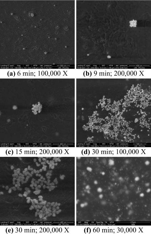
Figure 2: Photomicrographs of natural rubber samples with incorporated gold nanoparticles obtained by scanning electron microscopy. Reduction time of the nanoparticles in the sample is given in each Figure, as well as the magnification factor.

Figure 2(a) exemplifies MLSS application using the last starlet resolution level $L=10$. Thus, MLSS generates seven segmentation levels ($R_{w}=\{R_{3},\ldots,R_{10}\}$) (Figure 3). Gold nanoparticles appear in white, whereas background is shown in black. As $R$ increases, areas attributed to gold nanoparticles by MLSS tend to grow and merge, giving rise to larger regions. Segmentation levels $R_{6}$, $R_{7}$ and $R_{8}$ have a better visual representation of nanoparticles presented in this photomicrograph; lower levels contains fewer nanoparticle information, whereas in higher levels regions assigned to nanoparticles are fused, leading to misinterpretation of material surface.

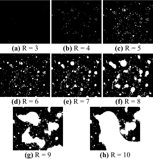
Figure 3: Results of Multi-Level Starlet Segmentation (MLSS) for Figure 2(a). Starlet lower levels represent smaller regions precisely. As the application level $R$ increases areas detected by MLSS tend to merge, creating larger regions.

After MLSS application, each $R_{W}$ element is compared to its corresponding GT (Figure 4) thus acquiring TP, FP, FN and TN (Section 2.4). MCC (Equation 8) is calculated for all $R_{W}$ elements (Table 1) from these parameters, and their values were compared. This comparison will determine the optimal segmentation level.

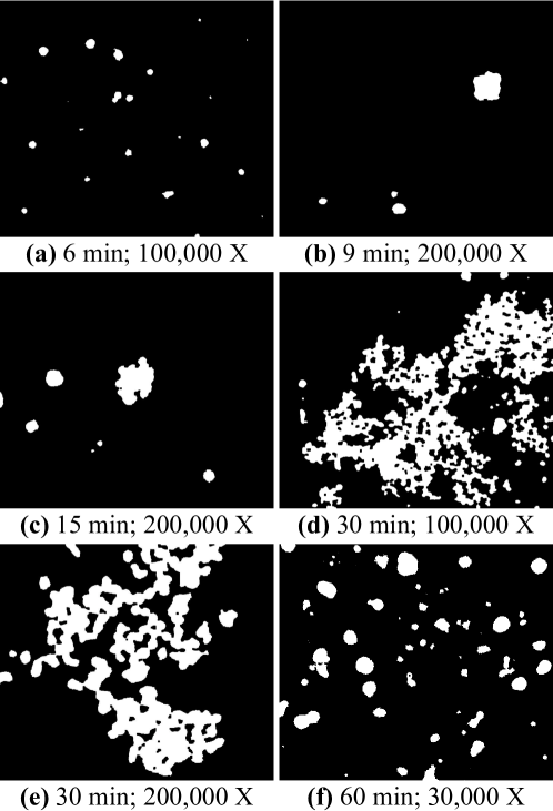
Figure 4: Ground Truth (GT) of Figure 2 photomicrographs. These images were obtained by a specialist, and represent gold nanoparticles in a sample surface.

Table 1: MCC obtained from Equation 8 application in NR/Au samples (Figure 2) for levels $R_{3}$ to $R_{10}$. Higher MCC values for each photomicrography are shown in red. $R_{7}$ was chosen as the optimal segmentation level for Figure 2 images, according to MCC values.

	MCC (%)
Reduction time (min); Magnification ($\bm{\times}$)	$R_{3}$	$R_{4}$	$R_{5}$	$R_{6}$	$R_{7}$	$R_{8}$	$R_{9}$	$R_{10}$
6; $\bm{100,000}$	5.342	22.382	32.335	36.172	34.039	27.096	17.031	10.646
9; $\bm{200,000}$	2.302	25.040	30.712	39.613	49.271	47.863	34.236	18.007
15; $\bm{200,000}$	7.642	31.534	49.005	65.083	72.195	63.440	48.205	28.944
30; $\bm{100,000}$	15.662	39.251	46.976	55.753	63.359	67.580	65.125	59.147
30; $\bm{200,000}$	4.314	32.183	53.876	65.137	72.593	70.222	65.261	52.300
60; $\bm{30,000}$	0	8.841	26.021	42.144	51.235	56.591	45.687	33.489

Best MCC values for Figure 2 images are given for segmentation levels $R_{6}$ (one time), $R_{7}$ (three times), and $R_{8}$ (two times); furthermore, the difference of sixth/eighth segmentation levels with higher MCC, when compared to $R_{7}$, lies between $2.1\sim 5.4\%$. Based on these facts, $R_{7}$ is elected the optimal level for MLSOS application in dataset photomicrographs. In order to confirm $R_{7}$ as the optimal segmentation level, precision, recall and accuracy values for $R_{6}$, $R_{7}$ and $R_{8}$ were obtained and compared (Table 2). It can be seen that precision and recall values tend to decrease and increase, respectively, as segmentation levels become higher.

Table 2: Precision, recall and accuracy values (Equation 9) obtained by applying the proposed methodology in Figure 2 fotomicrographs (segmentation levels $R_{6}$, $R_{7}$, $R_{8}$). Higher values for accuracy, for each image, are given in red.

	Precision (%)			Recall (%)			Accuracy (%)
Reduction time (min); Magnification ($\bm{\times}$)	$R_{6}$	$R_{7}$	$R_{8}$	$R_{6}$	$R_{7}$	$R_{8}$	$R_{6}$	$R_{7}$	$R_{8}$
6; $\bm{100,000}$	86.639	49.675	16.970	52.425	88.695	97.446	99.188	98.525	93.011
9; $\bm{200,000}$	26.887	28.491	24.093	62.133	89.018	99.750	96.983	96.581	95.412
15; $\bm{200,000}$	65.648	54.820	41.941	66.385	97.393	99.746	98.184	97.798	96.325
30; $\bm{100,000}$	94.318	86.833	77.332	55.154	74.186	90.388	84.813	88.314	88.616
30; $\bm{200,000}$	85.822	81.991	67.341	62.612	78.389	94.300	86.493	89.012	85.445
60; $\bm{30,000}$	36.733	39.366	39.066	62.183	80.243	95.363	88.808	88.929	88.155

$R_{6}$ and $R_{7}$ are the levels with higher accuracy values. In cases where accuracy is higher for $R_{6}$, the difference compared with their respective $R_{7}$ values is lower than $0.7\%$. Therefore $R_{7}$ is a suitable choice of the optimal level.

After choosing the optimal segmentation level, dataset images were processed using MLSOS. An example of the obtained segmentation using $R_{7}$ is given for Figure 2 photomicrographs (Figure 5).

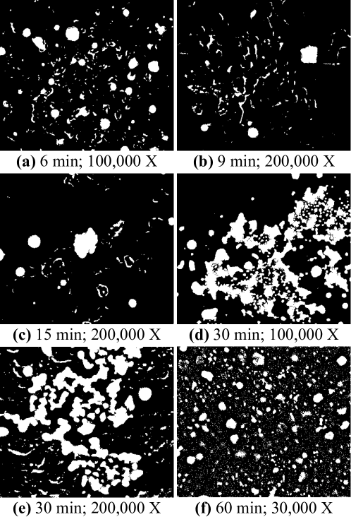
Figure 5: Result of Multi-Level Starlet Optimal Segmentation (MLSOS) application in Figure 2 photomicrographs. Optimal level: $R_{7}$.

A visual comparison between Figure 2 ground truths (Figure 4) and the result of MLSOS application (Figure 5) is based on TP, FP, FN and TN (Figure 6), where green, blue and red represent TP, FN and FP pixels, respectively. MLSOS defines some surface defects of the material as areas with nanoparticles; such behavior is represented by shapeless red areas in this comparison. Apparently, $R_{7}$ is not sufficient for segmenting nanoparticles contained in larger sets. This phenomenon is shown by the concentration of FN pixels (blue regions) appearing mostly contained in sets of TP pixels (green areas).

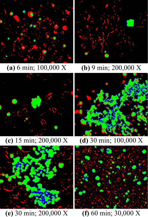
Figure 6: Comparison between ground truths (Figure 4) and Multi-Level Starlet Optimal Segmentation (MLSOS, Figure 5) for photomicrographs of Figure 2. Green: TP pixels; blue: FN pixels; red: FP pixels. Shapeless red areas are attributed to defects in the material surface.

Since MLSOS results were acquired, Equation 10 can be applied for the estimation of nanoparticles in photomicrographs (Section 2.7, Figure 7). Each set was separated according to its magnification, containing photomicrographs related to the reduction time. Thereby the behavior of incorporated gold nanoparticles in a rubber sample can be evaluated according to reduction time.

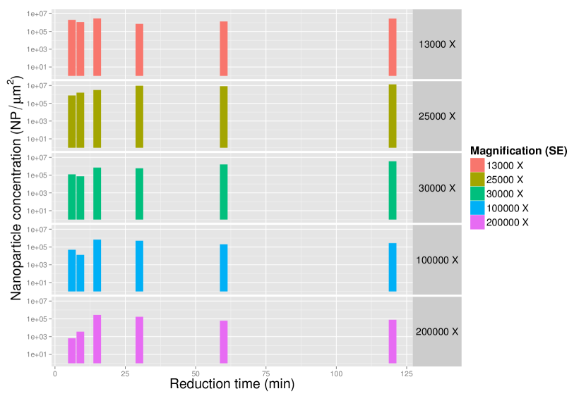
Figure 7: Area attributed to gold nanoparticles using Multi-Level Starlet Optimal Segmentation (MLSOS) in $13,000\times$ to $200,000\times$ image sets ($R_{7}$, secondary detector). The bars represent the nanoparticle amount by $\mu m^{2}$ for different gold reduction times, namely: 6, 9, 15, 30, 60 and 120 minutes, for each magnification.

MLSOS results are compared to temporal evolution of nanoparticles incorporation on the surface of natural rubber samples, measured in terms of increase in the maximum of the plasmon absorption band due to reduction time. These measures were performed as a comparative basis for membranes prepared from latex obtained from different collections, conducted at different times of the year, evaluated by ultraviolet-visible spectroscopy (UV-Vis, Figure 8), where black dots represent NR/Au samples absorbance. The red line and the shaded area presents, respectively, mean and standard deviation evolution between samples with same reduction time.

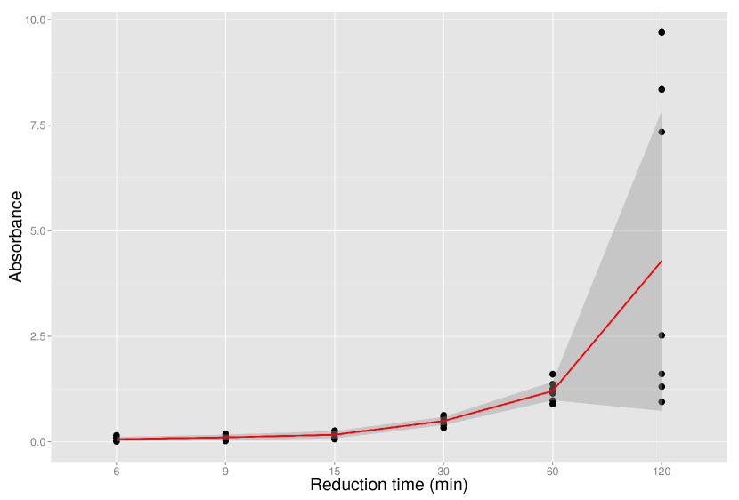
Figure 8: Temporal evolution from incorporation of gold nanoparticles on the surface of natural rubber membranes, measured in terms of increase in the maximum of the absorption band due to reduction time. Black dots: NR/Au samples absorbance. Red line: mean evolution. Shaded area: standard deviation evolution.

As shown in UV-Vis measures, temporal evolution presents an increase depending on the reduction time. This increase in intensity of absorption bands is given by the rise in the amount of gold nanoparticles deposited on natural rubber surface, that could generate nanoparticle aggregates mainly observed after the reduction time of 30 minutes [7]. Reliable reproducibility of results is given up to the reduction time of 60 minutes, given the small standard deviation obtained from comparison of different samples. These results indicate also a reduction timeout of 120 minutes, whereas some samples exceeds absorbance measuring limit of the equipment due to the formation of a thick layer of nanoparticles and aggregated bulk, decreasing the reproducibility of results.

Nevertheless, it is necessary to remark that electron microscopy only evaluates nanoparticles in the surface of natural rubber membranes, whereas UV-Vis spectroscopy evaluates all deposited nanoparticles between the optical analysis path, since it was previously demonstrated that particles could be incorporated within 3 micrometers in the volume of natural rubber membranes [6].

According to nanoparticle evaluation through MLSOS (Figure 7),

• $13,000\times$: concentration oscillates along reduction time. This scenario occurs due to the amount of blurred points in photomicrographs corresponding to this magnification (namely 6, 60 and 120 minutes); this fact can also be attributed to the small amount of nanoparticles contained in the photomicrograph for the reduction time of 9 minutes. The higher concentration of nanoparticles in 15 minutes is attributed to the evaluation of an area with nanoparticles accumulated on the surface, for better comprehension of size and shape of formed nanoparticles. However, in 30 and 120 minutes it is possible to observe the increase of gold nanoparticles incorporated in the surface of natural rubber, equally presented by UV-Vis spectroscopy results.

• $25,000\times$: concentration increases logarithmically, tending to stability. This image set presents a coherent behavior when comparing to Figure 8, reaching a plateau at 60 minutes; it is possible to observe in related studies [7] that nanoparticle growth occurs out of the natural rubber plane from this reduction time, forming aggregates of nanoparticles, difficulting the total nanoparticle evaluation in the natural rubber surface. This difficulty is solved increasing SEM magnification to $200,000\times$. Areas with higher contrast in samples of 9 and 120 minutes were labeled with a lower accuracy degree.

• $30,000\times$: concentration appears to behave as in $25,000\times$, but there is a small oscillation. This contrast difference affects photomicrographs corresponding to 6 and 30 minutes. Nanoparticle amount increase after 30 minutes.

• $100,000\times$: concentration tends to stability after 15 minutes. The amount of nanoparticles in 6 minutes appears to be higher than 9 minutes; this situation occurs because surface defects are attributed to nanoparticles through MLSOS. Similarly, blurred areas in 60 and 120 photomicrographs affects the final result.

• $200,000\times$: concentration behavior resembles that of $100,000\times$. Superficial details were assigned to nanoparticles in photomicrographs of 6 and 9 minutes. Besides, photomicrographs corresponding to 60 and 120 minutes have blurred areas, affecting MLSOS performance.

4 Conclusion

In this study we consolidate Multi-Level Starlet Segmentation (MLSS) and Multi-Level Starlet Optimal Segmentation (MLSOS), techniques presented to automatic separate information in photomicrographs. MLSS performs separation of areas in several levels, whereas MLSOS chooses the optimal segmentation level based on Matthews correlation coefficient (MCC). Segmentation reliability is evaluated by precision, recall and accuracy measures.

MLSOS is applied to estimate the amount of gold nanoparticles incorporated in a natural rubber sample, using five photomicrograph sets with different magnifications. The samples were obtained by green synthesis of gold nanoparticles using natural rubber membranes, in different reduction times. This technique can be used in the investigation of chemical kinetics in the synthesis of nanoparticles, and also as a complement of UV-Vis spectroscopy, based on image datasets.

Segmentation results were compared to UV-Vis spectroscopy, achieving satisfactory results mainly in the image set with magnification of $25,000\times$. Issues in segmentation are related to surface defects being recognized as nanoparticles by MLSOS. However, even in these cases MLSOS presents accuracy higher than 88%.

References

- [1] Annamalai A, Christina VLP, Sudha D, Kalpana M, Lakshmi PTV (2013) Green synthesis, characterization and antimicrobial activity of Au NPs using Euphorbia hirta L. leaf extract. Colloid Surface B 108:60–65. doi:10.1016/j.colsurfb.2013.02.012
- [2] Aromal SA, Philip D (2012) Green synthesis of gold nanoparticles using Trigonella foenum-graecum and its size-dependent catalytic activity. Spectrochim Acta A 97:1–5. doi:10.1016/j.saa.2012.05.083
- [3] Baldi P, Brunak S, Chauvin Y, Andersen CAF, Nielsen H (2000) Assessing the accuracy of prediction algorithms for classification: an overview. Bioinformatics 16(5):412–424. doi:10.1093/bioinformatics/16.5.412
- [4] Barboza-Filho CG, Cabrera FC, dos Santos RJ, de Saja Saez JA, Job AE (2012) The influence of natural rubber/Au nanoparticle membranes on the physiology of Leishmania brasiliensis. Exp Parasitol 130(2):152–158. doi:10.1002/jrs.3074
- [5] Cabrera FC, Aoki PHB, Aroca RF, Constantino CJL, dos Santos DS, Job AE (2012) Portable smart films for ultrasensitive detection and chemical analysis using SERS and SERRS. J Raman Spectrosc 43(4):474–477. doi:10.1002/jrs.3074
- [6] Cabrera FC, Mohan H, dos Santos RJ, Agostini DLS, Aroca RF, Rodríguez-Pérez MA, Job AE (2013) Green Synthesis of Gold Nanoparticles with Self-Sustained Natural Rubber Membranes. J Nanomat 2013:10. doi:10.1155/2013/710902
- [7] Cabrera FC, Agostini DLS, dos Santos RJ, Teixeira SR, Rodriguez-Perez MA, Job AE (2013) Characterization of natural rubber/gold nanoparticles SERS-active substrate. J Appl Polym Sci 130(1):186–192. doi:10.1002/app.39153
- [8] de Siqueira AF, Cabrera FC, Pagamisse A, Job AE (2014) Segmentation of scanning electron microscopy images from natural rubber samples with gold nanoparticles using starlet wavelets. Microsc Res Techniq 77(1):71–78. doi:10.1002/jemt.22314
- [9] de Siqueira AF, Nakasuga WM, Pagamisse A, Job AE (2014) An automatic method for segmentation of fission tracks in epidote crystal photomicrographs. Comput Geosci 69:55–61. doi:10.1016/j.cageo.2014.04.008
- [10] Gajanan G, Chang M, Kim J, Jin E (2011) Biogenic materialization using pear extract intended for the synthesis and design of ordered gold nanostructures. J Mater Sci 46(14):4741–4747. doi:10.1007/s10853-011-5384-0
- [11] Genovesio A, Olivo-Marin J-C (2003) Tracking fluroescent spots in biological video microscopy. In: Conchello J-A, Cogswell, CJ, Wilson T (ed) Proc. SPIE 4964, Three-Dimensional and Multidimensional Microscopy: Image Acquisition and Processing X. SPIE, San Jose, pp 98–105. doi:10.1117/12.478040
- [12] Holschneider M, Kronland-Martinet R, Morlet J, Tchamitchian P (1990) A Real-Time Algorithm for Signal Analysis with the Help of the Wavelet Transform. In: Combes J-M, Grossmann A, Tchamitchian P (ed) Wavelets: Time-Frequency Methods and Phase Space Proceedings of the International Conference, Marseille, France, December 14–18, 1987, Springer, Berlin, pp. 286–297
- [13] Kannan D, Tapobrata P (2014) Synthesis of Gold Nanoparticles from Different Cellular Fractions of Fusarium oxysporum. J Nanosci Nanotechnol 14(5):3455–3463. doi:10.1166/jnn.2014.8247
- [14] Kumar VG, Gokavarapu SD, Rajeswari A, Dhas TS, Karthick V, Kapadia Z, Shrestha T, Barathy IA, Roy A, Sinha S (2011) Facile green synthesis of gold nanoparticles using leaf extract of antidiabetic potent Cassia auriculata. Colloid Surface B 87(1):159–63. doi:10.1016/j.colsurfb.2011.05.016
- [15] Lin J, Zhou ZJ, Li ZM, Zhang CL, Wang XS, Wang K, Gao G, Huang P, Cui DX (2013) Biomimetic one-pot synthesis of gold nanoclusters/nanoparticles for targeted tumor cellular dual-modality imaging. Nanoscale Research Letters 8:170–176. doi:10.1186/1556-276X-8-170
- [16] Liu J-M, Chen J-T, Yan X-P (2013) Near Infrared Fluorescent Trypsin Stabilized Gold Nanoclusters as Surface Plasmon Enhanced Energy Transfer Biosensor and in Vivo Cancer Imaging Bioprobe. Anal Chem 85:3238–3245. doi:10.1021/ac303603f
- [17] Matthews BW (1975) Comparison of the predicted and observed secondary structure of T4 phage lysozyme. Biochim Biophys Acta 405:442–451. doi:10.1016/0005-2795(75)90109-9
- [18] Nagajyothi PC, Lee KD, Sreekanth TVM (2014) Biogenic Synthesis of Gold Nanoparticles (Quasi-Spherical, Triangle, and Hexagonal) Using Lonicera Japonica Flower Extract and Its Antimicrobial Activity. Syn React Inorg Met Nano 44(7):1011–1018. doi:10.1080/15533174.2013.797456
- [19] Noruzi M, Zare D, Khoshnevisan K, Davoodi D (2011) Rapid green synthesis of gold nanoparticles using Rosa hybrida petal extract at room temperature. Spectrochim Acta A 79(5):1461–1465. doi:10.1016/j.saa.2011.05.001
- [20] Olson DL, Delen D (2008) Advanced data mining techniques. Springer, Berlin
- [21] Parial D, Patra HK, Dasgupta AKR, Pal R (2012) Screening of different algae for green synthesis of gold nanoparticles. Eur J Phycol 47(1):22–29. doi:10.1080/09670262.2011.653406
- [22] Shensa MJ (1992) The discrete wavelet transform: Wedding the a trous and Mallat algorithms. IEEE T Signal Proces 40(10):2464–2482. doi:10.1109/78.157290
- [23] Starck J-L, Murtagh F (2006) Astronomical image and data analysis. Springer, Berlin
- [24] Starck J-L, Murtagh F, Bertero M (2011) Starlet Transform in Astronomical Data Processing. In: Scherzer O (ed) Handbook of Mathematical Methods in Imaging. Springer, New York, pp. 1489–1531
- [25] Starck J-L, Murtagh F, Fadili JM (2010) Sparse image and signal processing: wavelets, curvelets, morphological diversity. Cambridge University Press, New York
- [26] Sujitha MV, Kannan S (2013) Green synthesis of gold nanoparticles using Citrus fruits (Citrus limon, Citrus reticulata and Citrus sinensis) aqueous extract and its characterization. Spectrochim Acta A 102:15–23. doi:10.1016/j.saa.2012.09.042
- [27] Vijayakumar R, Devi V, Adavallan K, Saranya D (2011) Green synthesis and characterization of gold nanoparticles using extract of anti-tumor potent Crocus sativus. Physica E 44(3):665–671. doi:10.1016/j.physe.2011.11.002
- [28] Wang Q, Yuan Y, Yan P, Li X (2013) Saliency detection by multiple-instance learning. IEEE T Cybernetics 43(2):660–672. doi:10.1109/TSMCB.2012.2214210
- [29] Witten IH, Frank E, Hall MA (2011) Data Mining: Practical Machine Learning Tools and Techniques. Morgan Kaufmann Publishers, San Francisco