A Joint Sparse Recovery Framework for Accurate Reconstruction of Inclusions in Elastic Media

Abstract

A robust algorithm is proposed to reconstruct the spatial support and the Lamé parameters of multiple inclusions in a homogeneous background elastic material using a few measurements of the displacement field over a finite collection of boundary points. The algorithm does not require any linearization or iterative update of Green’s function but still allows very accurate reconstruction. The breakthrough comes from a novel interpretation of Lippmann-Schwinger type integral representation of the displacement field in terms of unknown densities having common sparse support on the location of inclusions. Accordingly, the proposed algorithm consists of a two-step approach. First, the localization problem is recast as a joint sparse recovery problem that renders the densities and the inclusion support simultaneously. Then, a noise robust constrained optimization problem is formulated for the reconstruction of elastic parameters. An efficient algorithm is designed for numerical implementation using the Multiple Sparse Bayesian Learning (M-SBL) for joint sparse recovery problem and the Constrained Split Augmented Lagrangian Shrinkage Algorithm (C-SALSA) for the constrained optimization problem. The efficacy of the proposed framework is manifested through extensive numerical simulations. To the best of our knowledge, this is the first algorithm tailored for parameter reconstruction problems in elastic media using highly under-sampled data in the sense of Nyquist rate.

AMS subject classifications 2000. Primary, 35R30, 74B05, 74J20, 78A46; Secondary, 15A29, 45Q05, 65F50, 94A12

Key words. elastic medium scattering, elasticity imaging, compressed sensing, joint sparsity, inverse scattering

1 Introduction

Elasticity imaging or elastography is a set of thriving non-invasive imaging techniques that have led to significant improvements in the quantitative evaluation and visualization of mechanical properties of elastic materials [5, 30]. It aims to recover spatial variations in certain material and geometric parameters of structures inside an elastic body from displacement data obtained non-invasively over a part of the boundary surface or inside the body using classical imaging modalities such as ultrasound, magnetic resonance, or speckle interferometry [44, 47, 48, 46]. Different terminologies (static, quasi-static, time-harmonic, and dynamic elasticity imaging) are used to differentiate techniques based on excitation mechanism adapted to probe the underlying elastic body [45].

Elasticity imaging frameworks cater to a broad range of applications, for example, non-destructive testing of elastic objects for material impurities and structural integrity [26], exploration geophysics for mineral reservoir prospecting [50, 53], and medical diagnosis, in particular, for detection and characterization of potential tumors of diminishing sizes [47, 48, 44]. In the perspectives of medical diagnosis elasticity imaging aims to fathom spatial variations in the material parameters of human tissues by harnessing the interdependence between elastic field and tissue elasticity. It can be perceived as a modernization of tissue palpation technique that has been used for centuries to identify abnormalities [46]. In fact, the correlation between changes in the stiffness of tissues with pathological phenomena, such as cirrhosis of the liver [36], weakening of vessel walls, and recruitment of collagen during tumorigenesis [28, 32, 54], has given an impetus to the quantitative characterization of underlying elastic properties using modern apparatus.

The inverse problem of quantitative evaluation of constitutive parameters is notorious for its complexity and ill-posed character. Many dedicated mathematical and computational algorithms for the reconstruction of location and parameters of anomalies of different geometrical nature (cavities, cracks, and inclusions) have been proposed over the past few decades (see, for instance, [1, 4, 6, 12, 13, 14, 15, 21, 26, 27, 29, 31, 33, 34, 42, 43, 55], the survey articles [16, 11], and the monograph [5]). Most of the classical techniques are suited to continuous measurements, in other words, to experimental setups allowing to measure continuum deformations inside the elastic body or on a substantial part of its boundary. In practice, this requires mechanical systems that furnish discrete data sampled on a very fine grid confirming to the Nyquist sampling rate. Unfortunately, this is not practically feasible due to mechanical, computational and financial constraints. On the other hand, several algorithms are based on linearizations with respect to the leading order of the scale factor of inclusions (for instance, asymptotic expansion methods [4, 7]), or the variations in the constitutive parameters. Born, Rytov and Foldy-Lax type approximations are also adopted. These simplifications are not always valid and are too strong to allow an accurate reconstruction. This results in a dramatic loss of image resolution and quality. The algorithms avoiding such assumptions usually require iterative updates and only a handful of direct reconstruction algorithms can be found in the literature. Specifically, these techniques are computationally very costly and are highly prone to instabilities as they require computation of numerous forward solutions for iterative updates and suffer from intrinsic ill-posedness of the problem [41]. In a nutshell, the existing results found in the literature are clearly not satisfactory from a practical point of view.

In this work, an accurate novel imaging algorithm is proposed for the reconstruction of multiple inclusions present in a bounded isotropic homogeneous elastic formation. It is assumed that a few measurements of the displacement field over a small finite set of boundary points are available. For simplicity, an elastostatic regime is considered, however, the quasi-static and time-harmonic elasticity problems are amenable to the same treatment with minor changes. One of the most important features of the proposed algorithm is that it does not require any linearization or iterative update of the Green’s function, yet it is felicitous to furnish the spatial support of the inclusions and their material parameters very accurately. The breakthrough comes from a novel interpretation of the Lippmann-Schwinger type integral representation of the displacement field that is derived in terms of unknown densities having jointly sparse spatial support on the location of inclusions. Therefore, the support identification problem can be recast as a joint sparse recovery problem for the unknown densities given that the support set of inclusions is itself sparse inside the elastic formation. This allows invoking a variety of compressed sensing signal recovery algorithms. Consequently, using any one of these algorithms, the solution of the joint sparse recovery problem can be obtained which yields not only the spatial support of the inclusions but also renders the unknown densities. The Lamé parameters of the inclusions are estimated using recovered densities in the second step of the proposed imaging framework by solving a linear inverse problem in sought parameters.

It is worthwhile mentioning that the additional information contained in the recovered densities is linked to the perturbed displacement and strain fields inside the support of the inclusions. The availability of the internal data and the sparsity assumption on the support of the inclusions thus compensate for the lack of over-determined measurements and significantly reduce the ill-posedness of the problem. In particular, this paves the way to a resolution enhancement since no linearization is applied in the proposed algorithm. Moreover, the numerical implementation of the proposed technique, as will be discussed later on in Section 5, does not require multiple forward solutions and is computationally very efficient. In fact, similar two-step approaches using joint sparse recovery formulations have been previously developed by our group for inverse scattering problems related to scalar Helmholtz equation [58], diffuse optical tomography [39, 40], and electric impedance tomography [38]. An extension to the electromagnetic inverse wave scattering governed by full Maxwell equations is on-going and has also provided very promising preliminary results. This extension will be reported elsewhere.

An important aspect of this work is the manifestation that even for elastic scattering problems, despite their complexity and ill-posedness, the derivation of an integral representation in terms of jointly sparse densities is possible that leads to an accurate and stable reconstruction with highly under-sampled data, which is not generally tractable by classical techniques. This clearly indicates, in view of the present investigation and the previously obtained results [58, 39, 40], that the proposed formulation may be so general that it provides a unified reconstruction framework for assorted inverse scattering problems.

The contents of this article are organized in the following order. The mathematical formulation of the inverse problem is provided in Section 2. The Lippmann-Schwinger type integral representation of the displacement field is derived in Section 3. Section 4 is dedicated to the joint sparse recovery based reconstruction algorithm. The computational aspects of the algorithm are discussed in Section 5. Several numerical experiments are conducted to substantiate the appositeness of the proposed technique in Section 6. The article ends with a summary of this investigation and a brief discussion provided in Section 7.

2 Mathematical formulation

In this section, the nomenclature and assumptions are specified that are adopted throughout this article and the mathematical formulation of the inverse problem dealt with in this article is provided.

2.1 Preliminaries and nomenclature

Consider an open bounded domain $\Omega\subset\mathbb{R}^{d}$, $d=2,3$, with connected $\mathcal{C}^{2}$-boundary $\partial\Omega$. Let us define $L^{2}(\Omega)$, $L^{\infty}(\Omega)$, $H^{1}(\Omega)$ and $H^{2}(\Omega)$ in the usual way endowed with standard norms. Let $H^{3/2}(\Omega)$ be defined as the interpolation space $[H^{1}(\Omega),H^{2}(\Omega)]_{1/2}$.

To facilitate the latter analysis, the subspace $L_{\Psi}^{2}(\partial\Omega)$ of $L^{2}(\partial\Omega)^{d}$ is defined by

$$L^{2}_{\Psi}(\partial\Omega):=\left\{{\bm{\varphi}}\in L^{2}(\partial\Omega)^{d}\,\Big{|}\,\int_{\partial\Omega}{\bm{\varphi}}\cdot{\bm{\psi}}d\sigma=0,\quad\forall{\bm{\psi}}\in\Psi\right\},$$

where $d\sigma$ denotes the infinitesimal surface element and $\Psi$ is the $d(d+1)/2$ dimensional vector space of infinitesimal rigid displacements, i.e.,

$$\Psi:=\left\{{\bm{\psi}}\in H^{1}(\Omega)^{d}\,\Big{|}\,\partial_{i}\psi_{j}+\partial_{j}\psi_{i}=0,\quad 1\leq i,j\leq d\right\}.$$

It is interesting to note that the vector space $\Psi$ contains constant functions and as a result

$$\int_{\partial\Omega}{\bm{\varphi}}d\sigma=0,\quad\forall{\bm{\varphi}}\in L^{2}_{\Psi}(\partial\Omega).$$

Let $\Omega$ be loaded with an isotropic homogeneous elastic material so that its stiffness tensor $\mathbb{C}^{0}=(C^{0}_{ijkl})_{i,j,k,l=1}^{d}$ is defined by

$$C^{0}_{ijkl}:=\lambda_{0}\delta_{ij}\delta_{kl}+\mu_{0}\left(\delta_{ik}\delta_{jl}+\delta_{il}\delta_{jk}\right),$$

where $\delta_{ij}$ is the Kronecker’s delta function, and constants $\lambda_{0}$ and $\mu_{0}$ are respectively the compression and shear moduli of the elastic material. It is assumed that these Lamé parameters satisfy the conditions

$$\mu_{0}>0\quad\text{and}\quad d\lambda_{0}+2\mu_{0}>0.$$ (2.1)

In fact, the conditions in (2.1) ensure the strong convexity of the stiffness tensor $\mathbb{C}^{0}$. Precisely, for all symmetric matrices $\mathbf{A}\in\mathbb{R}^{d\times d}\setminus\{\mathbf{0}\}$,

$$\left(\mathbb{C}^{0}:\mathbf{A}\right):\mathbf{A}\geq\min(2\mu_{0},d\lambda_{0}+2\mu_{0})\|\mathbf{A}\|_{F}^{2},$$

where the double dot operator $``:"$ (with varying definitions for $2-$, $3-$, or $4-$rank tensors by abuse of notation) and the Frobenius norm $\|\cdot\|_{F}$ are defined by

$$\mathbb{M}:\mathbf{A}:=\bigg{(}\sum_{k,l=1}^{d}m_{ijkl}a_{kl}\bigg{)}_{i,j=1}^{d},\quad\mathbf{A}:\mathbf{B}:=\sum_{i,j=1}^{d}a_{ij}b_{ij},\quad\text{and}\quad\|\mathbf{A}\|_{F}:=\sqrt{\mathbf{A}:\mathbf{A}},$$

for real matrices $\mathbf{A}=(a_{ij})_{i,j=1}^{d}$ and $\mathbf{B}=(b_{ij})_{i,j=1}^{d}$, and $4-$ rank tensors $\mathbb{M}=\left(m_{ijkl}\right)_{i,j,k,l=1}^{d}$.

Suppose that the material loaded in $\Omega$ contains $N\in\mathbb{N}$ open and bounded elastic inclusions $D_{n}$, $n=1,\cdots,N$, with simply connected smooth boundaries $\partial D_{n}$. To simplify the matters, the following assumptions are made throughout in this investigation.

1. All inclusions are separated apart from $\partial\Omega$ and their closures are mutually disjoint, i.e., there exists a constant $d_{0}\in\mathbb{R}_{+}$ such that

   $$\inf_{x\in\overline{D_{n}}}{\rm dist}(x,\partial\Omega)\geq d_{0}\quad\text{and}\quad\inf_{x\in\overline{D_{m}}}{\rm dist}(x,\overline{D_{n}})\geq d_{0},\quad\forall m\neq n,$$

   where dist represents the usual distance function in $\mathbb{R}^{d}$.

2. Each $D_{n}$ is isotropic but is allowed to be inhomogeneous so that its stiffness tensor, $\mathbb{C}^{n}({{\bf x}}):=(C^{n}_{ijkl}({{\bf x}}))_{i,j,k,l}^{d}$, is given by

   $$C^{n}_{ijkl}({{\bf x}}):=\lambda_{n}({{\bf x}})\delta_{ij}\delta_{kl}+\mu_{n}({{\bf x}})\left(\delta_{ik}\delta_{jl}+\delta_{il}\delta_{jk}\right),\qquad\forall\,{{\bf x}}\in D_{n},$$

   in terms of spatially varying Lamé parameters $\lambda_{n},\mu_{n}\in L^{\infty}(\Omega)$.

3. There exist constants $\underline{\lambda}_{n},\overline{\lambda}_{n},\underline{\mu}_{n},\overline{\mu}_{n}\in\mathbb{R}$ such that

   $$0<\underline{\mu}_{n}\leq\mu_{n}({{\bf x}})\leq\overline{\mu}_{n}\quad\text{and}\quad 0<d\underline{\lambda}_{n}+2\underline{\mu}_{n}\leq d\lambda_{n}({{\bf x}})+2\mu_{n}({{\bf x}})\leq d\overline{\lambda}_{n}+2\overline{\mu}_{n},$$

   for all ${{\bf x}}\in\overline{D_{n}}$ and $n\in\{1,\cdots,N\}$. By this assumption, It is ensured that, for all symmetric matrices $\mathbf{A}\in\mathbb{R}^{d\times d}\setminus\{\mathbf{0}\}$ and ${{\bf x}}\in D_{n}$,

   $$\max\left(2\overline{\mu}_{n},d\overline{\lambda}_{n}+2\overline{\mu}_{n}\right)\|\mathbf{A}\|_{F}^{2}\geq\;\left(\mathbb{C}^{n}({{\bf x}}):\mathbf{A}\right):\mathbf{A}\geq\;\min\left(2\underline{\mu}_{n},d\underline{\lambda}_{n}+2\underline{\mu}_{n}\right)\|\mathbf{A}\|_{F}^{2}.$$

4. The degenerate cases are avoided hereinafter by assuming that there exists a constant $\xi_{0}\in\mathbb{R}_{+}$ so that

   $$(\lambda_{0}-\lambda_{n}({{\bf x}}))(\mu_{0}-\mu_{n}({{\bf x}}))\geq\xi_{0},\quad\forall\,{{\bf x}}\in D_{n},\,\,n=1,\cdots,N.$$

   The assumption of uniform positivity is required to maintain the positivity of the elastic energy form involved in the Lippmann-Schwinger type representation of the scattered field presented in Section 3.2. By this, it is also ensured that the stiffness tensor,

   $$\mathbb{C}^{\star}({{\bf x}}):=\mathbb{C}^{0}\chi_{\Omega\setminus\cup_{n=1}^{N}\overline{D_{n}}}({{\bf x}})+\sum_{n=1}^{N}\mathbb{C}^{n}\chi_{D_{n}}({{\bf x}}),$$

   of $\Omega$ in the presence of inclusions, $D_{1},\cdots,D_{N}$, also satisfies strong convexity condition. Here $\chi_{D_{n}}$ represents the characteristic function of domain $D_{n}$.

To facilitate latter analysis, let us introduce piece-wise defined functions:

$$\lambda({{\bf x}}):=\sum_{n=1}^{N}\lambda_{n}({{\bf x}})\chi_{D_{n}}({{\bf x}}),\quad\mu({{\bf x}}):=\sum_{n=1}^{N}\mu_{n}({{\bf x}})\chi_{D_{n}}({{\bf x}}),\quad\text{and}\quad\mathbb{C}({{\bf x}}):=\sum_{n=1}^{N}\mathbb{C}^{n}({{\bf x}})\chi_{D_{n}}({{\bf x}}),$$

for all ${{\bf x}}\in\displaystyle\cup_{n=1}^{N}D_{n}$. Moreover, the following conventions will be used henceforth. Let $\mathbf{p}=(p_{i})_{i=1}^{d}$, $\mathbf{A}=(a_{ij})_{i,j=1}^{d}$ and $\mathbf{B}=(b_{ijk})_{i,j,k=1}^{d}$ be respectively any arbitrary vector, a matrix and a $3-$rank tensor. Let $\mathbf{H}:\mathbb{R}^{d}\to H^{1}(\Omega)^{d\times d}$, ${{\bf x}}\mapsto(h_{ij}({{\bf x}}))_{i,j=1}^{d}$ be any matrix valued function and $({\hat{\itbf e}}_{1},\cdots,{\hat{\itbf e}}_{d})$ be the standard basis in $\mathbb{R}^{d}$. Then, for all $i,j,k\in\{1,\cdots,d\}$,

$$\mathbf{A}\cdot\mathbf{p}:=\sum_{i,j}a_{ij}p_{j}{\hat{\itbf e}}_{i}\quad\text{and}\quad\mathbf{B}:\mathbf{A}:=\sum_{i,j,k}b_{ijk}a_{jk}{\hat{\itbf e}}_{i},$$

$$\nabla\cdot\mathbf{H}({{\bf x}}):=\sum_{i,j}\left(\frac{\partial h_{ij}}{\partial x_{i}}({{\bf x}})\right){\hat{\itbf e}}_{j},\quad\left[\nabla\mathbf{H}({{\bf x}})\right]_{ijk}:=\frac{\partial h_{ij}}{\partial x_{k}}({{\bf x}}),\quad\text{and}\quad\left[\left(\nabla\mathbf{H}({{\bf x}})\right)^{\top}\right]_{ijk}:=\frac{\partial h_{ik}}{\partial x_{j}}({{\bf x}}),$$

where superposed $\top$ indicates the transpose operation and the notation $[\cdot]$ is used to denote any component of a tensor, matrix or vector (e.g., $[\mathbf{p}]_{2}=p_{2}$ for a vector $\mathbf{p}\in\mathbb{R}^{d}$). The operators ${slice}_{1}:\{1,\cdots,d\}\times\mathbb{R}^{d\times d\times d}\to\mathbb{R}^{d\times d}$ and $vec:\mathbb{R}^{d\times d}\to\mathbb{R}^{d^{2}}$, defined by

$${\rm slice}_{1}(i,\mathbf{B}):=\left(b_{ijk}\right)_{j,k=1}^{d}\,\,\text{(for fixed $i$)}\quad\text{and}\quad{\rm vec}(\mathbf{A}):=\begin{pmatrix}\mathbf{a}_{1}^{\top},&\cdots,&\mathbf{a}_{d}^{\top}\end{pmatrix}^{\top},$$

will be useful in the sequel. Here $\mathbf{a}_{i}$ denotes the $i-$th column of matrix $\mathbf{A}$. Finally,

$${\rm diag}(r_{1},\cdots,r_{\ell})\in\mathbb{R}^{\ell\times\ell},\qquad\ell\in\mathbb{N},$$

will represent a diagonal matrix with diagonal elements $r_{1},\cdots,r_{\ell}\in\mathbb{R}$.

2.2 Problem formulation

Let ${{\bf u}}_{m}:\overline{\Omega}\to\mathbb{R}^{d}$, for each $m=1,\cdots,M\in\mathbb{N}$, be the displacement field in $\Omega$, in the presence of $D_{1},\cdots,D_{N}$, caused by an applied surface traction $\mathbf{g}_{m}\in L^{2}_{\Psi}(\partial\Omega)$ on its boundary $\partial\Omega$. Then, the vector field ${{\bf u}}_{m}$ is the solution to

$$\begin{cases}\displaystyle\nabla\cdot\left(\mathbb{C}^{\star}:\mathcal{E}[{{\bf u}}_{m}]\right)=\mathbf{0},&\text{in}\;\;\Omega,\\ \left(\mathbb{C}^{0}:\mathcal{E}[{{\bf u}}_{m}]\right)\cdot\bm{\nu}=\mathbf{g}_{m},&\text{on}\;\;\partial\Omega,\end{cases}$$ (2.2)

where ${{\bf u}}_{m}\in H^{1}(\Omega)$ such that ${{\bf u}}_{m}\big{|}_{\partial\Omega}\in L^{2}_{\Psi}(\partial\Omega)$ in order to ensure the existence of a unique weak solution. Here $\bm{\nu}$ is the outward unit normal to $\partial\Omega$ and $\mathcal{E}({{\bf u}}_{m})$ denotes the strain tensor related to ${{\bf u}}_{m}$ and is given by $\mathcal{E}[{{\bf u}}_{m}]:=(\nabla{{\bf u}}_{m}+\nabla{{\bf u}}_{m}^{\top})/2.$

For convenience, the linear isotropic elasticity operator and the corresponding surface traction operator associated with $\mathbb{C}^{0}$ will be usually denoted by $\mathcal{L}_{\lambda_{0},\mu_{0}}$ and ${\partial}/{\partial\bm{\nu}}$ respectively, i.e., for any smooth function ${{\bf w}}:\mathbb{R}^{d}\to\mathbb{R}^{d}$,

$$\mathcal{L}_{\lambda_{0},\mu_{0}}[{{\bf w}}]:=\nabla\cdot\left(\mathbb{C}^{0}:\mathcal{E}[{{\bf w}}]\right),$$

$$\frac{\partial{{\bf w}}}{\partial\bm{\nu}}:=\left(\mathbb{C}^{0}:\mathcal{E}[{{\bf w}}]\right)\cdot\bm{\nu}=\lambda_{0}(\nabla\cdot{{\bf w}})\bm{\nu}+2\mu_{0}\mathcal{E}({{\bf w}})\cdot\bm{\nu}.$$

Similarly, analogous notation, $\mathcal{L}_{\lambda,\mu}$ and $\partial/\partial\widetilde{\bm{\nu}}$, will be used for operators corresponding to $\mathbb{C}$ (i.e., to $\lambda$ and $\mu$). Moreover, a de facto extension of these operators will be used for matrix valued functions by invoking conventions listed in Section 2.1.

It can be easily verified that the problem (2.2) is equivalent to the transmission problem

$$\begin{cases}\mathcal{L}_{\lambda_{0},\mu_{0}}[{{\bf u}}_{m}]=0,&\text{in }\Omega\setminus\cup_{n=1}^{N}\overline{D_{n}},\\ \mathcal{L}_{\lambda,\mu}[{{\bf u}}_{m}]=0,&\text{in }\cup_{n=1}^{N}{D_{n}},\\ {{\bf u}}_{m}{\big{|}_{-}}={{\bf u}}_{m}{\big{|}_{+}},&\text{on }\partial{D_{n}}\quad(\forall n=1,\cdots,N),\\ \displaystyle\frac{\partial{{\bf u}}_{m}}{\partial\widetilde{\bm{\nu}}}{\Big{|}_{-}}=\displaystyle\frac{\partial{{\bf u}}_{m}}{\partial\bm{\nu}}{\Big{|}_{+}},&\text{on }\partial{D_{n}}\quad(\forall n=1,\cdots,N),\\ \displaystyle\frac{\partial{{\bf u}}_{m}}{\partial\bm{\nu}}=\mathbf{g}_{m},&\text{on }\partial\Omega\quad\Big{(}{{\bf u}}_{m}\big{|}_{\partial\Omega}\in L^{2}_{\Psi}(\partial\Omega)\Big{)},\end{cases}$$ (2.3)

where subscripts $+$ and $-$ indicate the limiting values across the interface $\partial D_{n}$ from outside and from inside $D_{n}$ respectively, i.e., for any function ${{\bf w}}$,

$${{\bf w}}\big{|}_{\pm}({{\bf x}}):=\lim_{\epsilon\to 0^{+}}{{\bf w}}({{\bf x}}\pm\epsilon\bm{\nu}),\quad{{\bf x}}\in\partial D_{n}.$$

The background displacement field $\mathbf{U}_{m}$ in $\Omega$ (in the absence of any inclusion), caused by the surface traction $\mathbf{g}_{m}\in L^{2}_{\Psi}(\partial\Omega)$ applied on $\partial\Omega$, is also required. The vector field $\mathbf{U}_{m}:\overline{\Omega}\to\mathbb{R}^{d}$ is the solution to

$$\begin{cases}\mathcal{L}_{\lambda_{0},\mu_{0}}[\mathbf{U}_{m}]=0,&\text{in}\;\;\Omega,\\ \displaystyle\frac{\partial\mathbf{U}_{m}}{\partial\bm{\nu}}=\mathbf{g}_{m},&\text{on}\;\;\partial\Omega\quad\Big{(}\mathbf{U}_{m}\big{|}_{\partial\Omega}\in L^{2}_{\Psi}(\partial\Omega)\Big{)}.\end{cases}$$

The following inverse problem is dealt with in this article.

Inverse Problem

Let $\{{{\bf x}}_{r}\}_{r=1}^{R}\subset\partial\Omega$, for some $R\in\mathbb{N}$, be a finite collection of points on $\partial\Omega$. Let a known traction $\mathbf{g}_{m}\in L^{2}_{\Psi}(\partial\Omega)$, for each $m\in\{1,\cdots,M\in\mathbb{N}\}$, be applied on $\partial\Omega$ which induces the displacement fields ${{\bf u}}_{m}$ and $\mathbf{U}_{m}$ in $\Omega$, respectively, with and without the presence of inclusions, $D_{1},\cdots,D_{N}$. Given the set of measurements

$$\Big{\{}({{\bf u}}_{m}-\mathbf{U}_{m})({{\bf x}}_{r})\quad\Big{|}\quad r=1,\cdots,R,\;m=1,\cdots,M\Big{\}},$$

locate $D_{1},\cdots,D_{N}$ and reconstruct the corresponding Lamé parameters, $\lambda_{n}$ and $\mu_{n}$, for all $n=1,\cdots,N$.   

3 Lippmann-Schwinger type integral representation of perturbed displacement

The main ingredient of our reconstruction framework is a Lippmann-Schwinger type integral representation of the perturbations in the displacement fields, $({{\bf u}}_{m}-\mathbf{U}_{m})$, due to the presence of inclusions, $D_{1},\cdots,D_{N}$. In this section, an exact analytic formula is derived for the perturbations $({{\bf u}}_{m}-\mathbf{U}_{m})$ using tools mostly borrowed from the existing literature on integral equations. It is emphasized that similar Lippmann-Schwinger type formulations can be found in the literature; see, e.g., [49]. Nevertheless, the detailed derivation is provided in Section 3.2 for completeness sake as this formulation is the key component of our algorithm. Towards this end, it is best to pause and recall a few elements from layer potential theory for the linear elastostatic system in Section 3.1. The readers interested in further details are invited to read, for instance, the recent monograph [5].

3.1 Elements of layer potential theory for elastostatics

Let $\mathbf{\Gamma}$ denote the Kelvin matrix of fundamental solutions to the elastostatic system $\mathcal{L}_{\lambda_{0},\mu_{0}}$ in $\mathbb{R}^{d}$, i.e.,

$$\mathcal{L}_{\lambda_{0},\mu_{0}}[\mathbf{\Gamma}]({{\bf x}})=\delta_{\mathbf{0}}({{\bf x}})\mathbf{I}_{d},\qquad\forall\,{{\bf x}}\in\mathbb{R}^{d},$$ (3.1)

where $\mathbf{I}_{d}\in\mathbb{R}^{d\times d}$ is the identity matrix and $\delta_{\mathbf{0}}$ is the Dirac mass at $\mathbf{0}$. It is well known that (see, for instance, [8, Lemma 6.2])

$$\mathbf{\Gamma}({{\bf x}})=\begin{cases}\displaystyle\alpha\ln|{{\bf x}}|\mathbf{I}_{2}-\frac{\beta}{|{{\bf x}}|^{2}}{{\bf x}}{{\bf x}}^{\top},&\text{for}\;\;d=2,\\ \displaystyle-\frac{\alpha}{2|{{\bf x}}|}\mathbf{I}_{3}-\frac{\beta}{2|{{\bf x}}|^{3}}{{\bf x}}{{\bf x}}^{\top},&\text{for}\;\;d=3,\end{cases}$$

where the parameters $\alpha$ and $\beta$ are given by

$$\alpha:=\frac{\lambda_{0}+3\mu_{0}}{4\pi\mu_{0}(\lambda_{0}+2\mu_{0})}\quad\text{and}\quad\beta:=\frac{\lambda_{0}+\mu_{0}}{4\pi\mu_{0}(\lambda_{0}+2\mu_{0})}.$$ (3.2)

The double layer potential associated with operator $\mathcal{L}_{\lambda_{0},\mu_{0}}$ in $\Omega$, hereinafter denoted by $\mathcal{D}_{\Omega}$, is defined as

$$\mathcal{D}_{\Omega}[{\bm{\varphi}}]({{\bf x}}):=\int_{\partial\Omega}\frac{\partial}{\partial\bm{\nu}_{{\bf y}}}\mathbf{\Gamma}({{\bf x}}-{{\bf y}})\cdot{\bm{\varphi}}({{\bf y}})d\sigma({{\bf y}}),\qquad{{\bf x}}\in\mathbb{R}^{d}\setminus\partial\Omega,$$

for all ${\bm{\varphi}}\in L^{2}(\partial\Omega)^{d}$. Remind that, $\mathcal{D}_{\Omega}[{\bm{\varphi}}]$ is a solution to $\mathcal{L}_{\lambda_{0},\mu_{0}}\big{[}\mathcal{D}_{\Omega}[{\bm{\varphi}}]\big{]}=\mathbf{0}$ in $\mathbb{R}^{d}\setminus\partial\Omega$ for all ${\bm{\varphi}}\in L^{2}_{\Psi}(\partial\Omega)$ and the quantities $\mathcal{D}_{\Omega}[{\bm{\varphi}}]\big{|}_{\pm}$ are well-defined for all ${{\bf x}}\in\partial\Omega$. In fact, the following jump relations hold (see, e.g., [23])

$$\displaystyle\mathcal{D}_{\Omega}[{\bm{\varphi}}]\Big{|}_{\pm}({{\bf x}})=\left(\mp\frac{1}{2}\mathcal{I}+\mathcal{K}_{\Omega}\right){\bm{\varphi}}({{\bf x}}),\qquad{\rm a.e.}\quad{{\bf x}}\in\partial\Omega,$$ (3.3)

where $\mathcal{I}:L^{2}(\partial\Omega)^{d}\to L^{2}(\partial\Omega)^{d}$ is the identity map and $\mathcal{K}_{\Omega}$ is the so-called Neumann-Poincaré operator, defined by

$$\mathcal{K}_{\Omega}[{\bm{\varphi}}]({{\bf x}}):={\rm p.v.}\displaystyle\int_{\partial\Omega}\frac{\partial}{\partial\bm{\nu}_{{\bf y}}}\mathbf{\Gamma}({{\bf x}}-{{\bf y}})\cdot{\bm{\varphi}}({{\bf y}})d\sigma({{\bf y}}),\quad{\rm a.e.}\quad\,{{\bf x}}\in\partial\Omega,$$

for all ${\bm{\varphi}}\in L^{2}(\partial\Omega)^{d}$. Here p.v. stands for the Cauchy principle value.

Let $\mathbf{N}(\cdot,{{\bf y}}):\overline{\Omega}\to\mathbb{R}^{d\times d}$, for a fixed ${{\bf y}}\in\overline{\Omega}$, be the Neumann function for the background domain $\Omega$ without any inclusion, i.e., the weak solution to

$$\begin{cases}\mathcal{L}_{\lambda_{0},\mu_{0}}[\mathbf{N}]({{\bf x}},{{\bf y}})=-\delta_{{\bf y}}({{\bf x}})\mathbf{I}_{d},&\text{for }{{\bf x}}\in\Omega,\\ \displaystyle\frac{\partial\mathbf{N}}{\partial\bm{\nu}_{{\bf x}}}({{\bf x}},{{\bf y}})=-\frac{1}{|\partial\Omega|}\mathbf{I}_{d},&\text{for }{{\bf x}}\in\partial\Omega,\end{cases}$$ (3.4)

subject to the condition $\mathbf{N}(\cdot,{{\bf y}})\in L^{2}_{\Psi}(\partial\Omega)$, for all ${{\bf y}}\in\overline{\Omega}$.

The following result from [8, Lemma 6.16] is of great significance in the latter analysis.

Lemma 3.1.

For all ${{\bf x}}\in\partial\Omega$ and ${{\bf y}}\in\Omega$,

$$\left(-\displaystyle\frac{1}{2}\mathcal{I}+\mathcal{K}_{\Omega}\right)[\mathbf{N}(\cdot,{{\bf y}})]({{\bf x}})=\mathbf{\Gamma}({{\bf x}},{{\bf y}})\quad\text{\rm modulo}\,\,\Psi.$$

Lemma 3.1 indicates that the operator $(-\mathcal{I}/2+\mathcal{K}_{\Omega})$ filters the effects of an imposed traction condition. It maps the solution of the elastostatic system in $\Omega$ with traction condition on $\partial\Omega$ to a solution of elastostatic system in $\mathbb{R}^{d}$ subject to radiation conditions. The operator $(-\mathcal{I}/2+\mathcal{K}_{\Omega})$ will be coined as Calderón preconditioner in the sequel and will be effectively used to design an efficient reconstruction algorithm.

3.2 Integral representation of perturbed displacement field

To facilitate the ensuing analysis, it is best to recall beforehand the Green’s identities corresponding to elastostatic system. These identities can be easily derived using integration by parts and the divergence theorem (see, for instance, [8, Sec. 9.1]).

• If ${{\bf v}}\in H^{1}(\Omega)^{d}$ and ${{\bf w}}\in H^{3/2}(\Omega)^{d}$ then

  $$\int_{\partial\Omega}{{\bf v}}\cdot\frac{\partial{{\bf w}}}{\partial\bm{\nu}}d\sigma=\int_{\Omega}{{\bf v}}\cdot\mathcal{L}_{\lambda_{0},\mu_{0}}[{{\bf w}}]d{{\bf x}}+\mathcal{Q}_{\Omega}^{\mathbb{C}^{0}}({{\bf v}},{{\bf w}}),$$ (3.5)

  where the quadratic (or so-called elastic energy) form $\mathcal{Q}_{\Omega}^{\mathbb{C}^{0}}:H^{1}(\Omega)^{d}\times H^{1}(\Omega)^{d}\to\mathbb{R}$ is defined by

  $$\mathcal{Q}_{\Omega}^{\mathbb{C}^{0}}({{\bf v}},{{\bf w}}):= \int_{\Omega}\mathcal{E}[{{\bf v}}]:\mathbb{C}^{0}:\mathcal{E}[{{\bf w}}]d{{\bf x}}$$

  $$= \int_{\Omega}\Big{[}\lambda_{0}(\nabla\cdot{{\bf v}})(\nabla\cdot{{\bf w}})+2\mu_{0}(\mathcal{E}[{{\bf v}}]:\mathcal{E}[{{\bf w}}])\Big{]}d{{\bf x}}.$$ (3.6)

  Once again, the de facto extension of $\mathcal{Q}^{\mathbb{C}^{0}}_{\Omega}$ is used if one of the arguments is a matrix, in which case it would furnish a vector field.

• If ${{\bf v}},{{\bf w}}\in H^{3/2}(\Omega)^{d}$ then the formula (3.5) leads to another Green’s identity

  $$\int_{\partial\Omega}\left({{\bf v}}\cdot\frac{\partial{{\bf w}}}{\partial\bm{\nu}}-{{\bf w}}\cdot\frac{\partial{{\bf v}}}{\partial\bm{\nu}}\right)d\sigma({{\bf x}})=\int_{\Omega}\left({{\bf v}}\cdot\mathcal{L}_{\lambda_{0},\mu_{0}}[{{\bf w}}]-{{\bf w}}\cdot\mathcal{L}_{\lambda_{0},\mu_{0}}[{{\bf v}}]\right)d{{\bf x}}.$$ (3.7)

  It is interesting to note that, by formula (3.7), if ${{\bf v}}$ is in addition a solution to $\mathcal{L}_{\lambda_{0},\mu_{0}}[{{\bf v}}]=\mathbf{0}$ in $\Omega$ then ${\partial{{\bf v}}}/{\partial\bm{\nu}}\in L^{2}_{\Psi}(\partial\Omega)$.

The first important result of this section is the following integral representation of the perturbed displacement field.

Lemma 3.2.

For all ${{\bf x}}\in\overline{\Omega}$,

$${{\bf u}}_{m}({{\bf x}})-\mathbf{U}_{m}({{\bf x}})=\int_{\cup_{n=1}^{N}D_{n}}\Big{[}\big{(}\lambda_{0}-\lambda({{\bf y}})\big{)} \big{(}\nabla_{{\bf y}}\cdot\mathbf{N}({{\bf x}},{{\bf y}})\big{)}\big{(}\nabla\cdot{{\bf u}}_{m}({{\bf y}})\big{)}$$

$$+2(\mu_{0}-\mu({{\bf y}}))\mathcal{E}[\mathbf{N}({{\bf x}},\cdot)]({{\bf y}}):\mathcal{E}[{{\bf u}}_{m}]({{\bf y}})\Big{]}d{{\bf y}}.$$ (3.8)

Proof.

Let us start with the representation,

$$\mathbf{U}_{m}({{\bf x}})=\int_{\partial\Omega}\mathbf{N}({{\bf x}},{{\bf y}})\cdot\mathbf{g}_{m}({{\bf y}})d\sigma({{\bf y}})=\int_{\partial\Omega}\mathbf{N}({{\bf x}},{{\bf y}})\cdot\frac{\partial{{\bf u}}_{m}}{\partial\bm{\nu}}({{\bf y}})d\sigma({{\bf y}}),\quad{{\bf x}}\in\overline{\Omega},$$

of the background solution $\mathbf{U}_{m}$. Note also that, by virtue of the imposed boundary condition on $\mathbf{N}$ and the fact that ${{\bf u}}_{m}\big{|}_{\partial\Omega}\in L^{2}_{\Psi}(\partial\Omega)$,

$$\int_{\partial\Omega}\frac{\partial}{\partial\bm{\nu}_{{\bf y}}}\mathbf{N}({{\bf x}},{{\bf y}})\cdot{{\bf u}}_{m}({{\bf y}})d\sigma({{\bf y}})=\mathbf{0},\quad{{\bf x}}\in\overline{\Omega}.$$

Therefore, the background field can be expressed as

$$\mathbf{U}_{m}({{\bf x}})=\int_{\partial\Omega}\left(\mathbf{N}({{\bf x}},{{\bf y}})\cdot\frac{\partial{{\bf u}}_{m}}{\partial\bm{\nu}}({{\bf y}})-\frac{\partial}{\partial\bm{\nu}_{{\bf y}}}\mathbf{N}({{\bf x}},{{\bf y}})\cdot{{\bf u}}_{m}({{\bf y}})\right)d\sigma({{\bf y}}),\quad{{\bf x}}\in\overline{\Omega}.$$

Consequently, a simple application of the Green’s formula (3.7) over $\Omega\setminus\cup_{n=1}^{N}\overline{D_{n}}$ furnishes

$$\mathbf{U}_{m}({{\bf x}})= -\int_{\Omega\setminus\cup_{n=1}^{N}\overline{D_{n}}}\Big{(}\mathcal{L}_{\lambda_{0},\mu_{0}}[\mathbf{N}]({{\bf x}},{{\bf y}})\cdot{{\bf u}}_{m}({{\bf y}})-\mathbf{N}({{\bf x}},{{\bf y}})\cdot\mathcal{L}_{\lambda_{0},\mu_{0}}[{{\bf u}}_{m}]({{\bf y}})\Big{)}d{{\bf y}}$$

$$+\sum_{n=1}^{N}\int_{\partial D_{n}}\left(\mathbf{N}({{\bf x}},{{\bf y}})\cdot\frac{\partial{{\bf u}}_{m}}{\partial\bm{\nu}}({{\bf y}})\Big{|}_{+}-\frac{\partial}{\partial\bm{\nu}_{{\bf y}}}\mathbf{N}({{\bf x}},{{\bf y}})\cdot{{\bf u}}_{m}({{\bf y}})\Big{|}_{+}\right)d\sigma({{\bf y}}),\quad{{\bf x}}\in\overline{\Omega}.$$ (3.9)

Remark that the second term on the right hand side (RHS) of (3.9) is identically zero thanks to the first equation in (2.3). Moreover, by invoking the transmission conditions on the displacement ${{\bf u}}_{m}$ and its surface traction on the boundaries $\partial D_{n}$ in (2.3), one obtains

$$\mathbf{U}_{m}({{\bf x}})= -\int_{\Omega\setminus\cup_{n=1}^{N}\overline{D_{n}}}\mathcal{L}_{\lambda_{0},\mu_{0}}[\mathbf{N}]({{\bf x}},{{\bf y}})\cdot{{\bf u}}_{m}({{\bf y}})d{{\bf y}}$$

$$+\sum_{n=1}^{N}\int_{\partial D_{n}}\left(\mathbf{N}({{\bf x}},{{\bf y}})\cdot\frac{\partial{{\bf u}}_{m}}{\partial\widetilde{\bm{\nu}}}({{\bf y}})\Big{|}_{-}-\frac{\partial}{\partial\bm{\nu}_{{\bf y}}}\mathbf{N}({{\bf x}},{{\bf y}})\cdot{{\bf u}}_{m}({{\bf y}})\Big{|}_{-}\right)d\sigma({{\bf y}}),\quad{{\bf x}}\in\overline{\Omega}.$$

By applying the Green’s identity (3.7) once again, but this time over $\cup_{n=1}^{N}D_{n}$, one gets

$$\mathbf{U}_{m}({{\bf x}})= -\int_{\Omega}\mathcal{L}_{\lambda_{0},\mu_{0}}[\mathbf{N}]({{\bf x}},{{\bf y}})\cdot{{\bf u}}_{m}({{\bf y}})d{{\bf y}}+\int_{\cup_{n=1}^{N}D_{n}}\mathbf{N}({{\bf x}},{{\bf y}})\cdot\mathcal{L}_{\lambda_{0},\mu_{0}}[{{\bf u}}_{m}]({{\bf y}})d{{\bf y}}$$

$$+\sum_{n=1}^{N}\int_{\partial D_{n}}\mathbf{N}({{\bf x}},{{\bf y}})\cdot\left(\frac{\partial{{\bf u}}_{m}}{\partial\widetilde{\bm{\nu}}}({{\bf y}})\Big{|}_{-}-\frac{\partial{{\bf u}}_{m}}{\partial\bm{\nu}}({{\bf y}})\Big{|}_{-}\right)d\sigma({{\bf y}}),\quad{{\bf x}}\in\overline{\Omega}.$$ (3.10)

Thanks to the first equation in (3.4) for the Neumann solution, one can easily identify the first term on the RHS of (3.10) as ${{\bf u}}_{m}({{\bf x}})$. Therefore,

$$\mathbf{U}_{m}({{\bf x}})-{{\bf u}}_{m}({{\bf x}})= \int_{\cup_{n=1}^{N}D_{n}}\mathbf{N}({{\bf x}},{{\bf y}})\cdot\mathcal{L}_{\lambda_{0},\mu_{0}}[{{\bf u}}_{m}]({{\bf y}})d{{\bf y}}$$

$$+\sum_{n=1}^{N}\int_{\partial D_{n}}\mathbf{N}({{\bf x}},{{\bf y}})\cdot\left(\frac{\partial{{\bf u}}_{m}}{\partial\widetilde{\bm{\nu}}}({{\bf y}})\Big{|}_{-}-\frac{\partial{{\bf u}}_{m}}{\partial\bm{\nu}}({{\bf y}})\Big{|}_{-}\right)d\sigma({{\bf y}}),\quad{{\bf x}}\in\overline{\Omega}.$$ (3.11)

On the other hand, by using Green’s identity (3.5) over $\cup_{n=1}^{N}D_{n}$, it is found that

$$\int_{\cup_{n=1}^{N}D_{n}}\mathbf{N}({{\bf x}},{{\bf y}})\cdot\mathcal{L}_{\lambda_{0},\mu_{0}}[{{\bf u}}_{m}]({{\bf y}})d{{\bf y}}= \sum_{n=1}^{N}\int_{\partial D_{n}}\mathbf{N}({{\bf x}},{{\bf y}})\cdot\frac{\partial{{\bf u}}_{m}}{\partial\bm{\nu}}({{\bf y}})\Big{|}_{-}d\sigma({{\bf y}})$$

$$-\mathcal{Q}_{\cup_{n=1}^{N}D_{n}}^{\mathbb{C}^{0}}\left(\mathbf{N}({{\bf x}},\cdot),{{\bf u}}_{m}\right),\quad{{\bf x}}\in\overline{\Omega}.$$

Consequently, a few fairly easy manipulations lead us to

$$\int_{\cup_{n=1}^{N}D_{n}}\mathbf{N}({{\bf x}},{{\bf y}})\cdot\mathcal{L}_{\lambda_{0},\mu_{0}}[{{\bf u}}_{m}]({{\bf y}})d{{\bf y}}= \sum_{n=1}^{N}\int_{\partial D_{n}}\mathbf{N}({{\bf x}},{{\bf y}})\cdot\left(\frac{\partial{{\bf u}}_{m}}{\partial\bm{\nu}}({{\bf y}})\Big{|}_{-}-\frac{\partial{{\bf u}}_{m}}{\partial\widetilde{\bm{\nu}}}({{\bf y}})\Big{|}_{-}\right)d\sigma({{\bf y}})$$

$$-\mathcal{Q}_{\cup_{n=1}^{N}D_{n}}^{\mathbb{C}^{0}-\mathbb{C}}(\mathbf{N}({{\bf x}},\cdot),{{\bf u}}_{m})$$

$$+\int_{\cup_{n=1}^{N}D_{n}}\mathbf{N}({{\bf x}},{{\bf y}})\cdot\mathcal{L}_{\lambda,\mu}[{{\bf u}}_{m}]({{\bf y}})d{{\bf y}},\quad{{\bf x}}\in\overline{\Omega},$$

wherein the last term vanishes thanks to the second equation in (2.3). Therefore,

$$\int_{\cup_{n=1}^{N}D_{n}} \mathbf{N}({{\bf x}},{{\bf y}})\cdot\mathcal{L}_{\lambda_{0},\mu_{0}}[{{\bf u}}_{m}]({{\bf y}})d{{\bf y}}+\sum_{n=1}^{N}\int_{\partial D_{n}}\mathbf{N}({{\bf x}},{{\bf y}})\cdot\left(\frac{\partial{{\bf u}}_{m}}{\partial\widetilde{\bm{\nu}}}({{\bf y}})\Big{|}_{-}-\frac{\partial{{\bf u}}_{m}}{\partial\bm{\nu}}({{\bf y}})\Big{|}_{-}\right)d\sigma({{\bf y}})$$

$$= -\mathcal{Q}_{\cup_{n=1}^{N}D_{n}}^{\mathbb{C}^{0}-\mathbb{C}}(\mathbf{N}({{\bf x}},\cdot),{{\bf u}}_{m}),\quad\forall{{\bf x}}\in\overline{\Omega}.$$ (3.12)

Finally, combining (3.11) and (3.12), it can be seen that

$${{\bf u}}_{m}({{\bf x}})-\mathbf{U}_{m}({{\bf x}})= \mathcal{Q}_{\cup_{n=1}^{N}D_{n}}^{\mathbb{C}^{0}-\mathbb{C}}(\mathbf{N}({{\bf x}},\cdot),{{\bf u}}_{m}),\quad{{\bf x}}\in\overline{\Omega}.$$

This leads to the conclusion together with the definition (3.6) of the quadratic form. ∎

The integral equation (3.8) provides an exact expression for the perturbations in the displacement field. However, it is important to note that the Neumann function $\mathbf{N}$ does not admit an exact explicit expression (except in a few trivial cases of simple domains such as disks and balls) in contrast to the Kelvin matrix $\mathbf{\Gamma}$ which is easily accessible. Therefore, although it is exact and valid for all ${{\bf x}}\in\overline{\Omega}$, the practical utility of the relation (3.8) is restricted. Nevertheless, a pre-processing of the data using Calderón preconditioner is particularly felicitous. In fact, by preconditioning integral equation (3.8) using $(-\mathcal{I}/2+\mathcal{K}_{\Omega})$ and invoking the Lemma 3.1, one can easily obtain an equivalent representation of the filtered measurements in terms of the Kelvin matrix. The following result is readily proved thanks to Lemmas 3.1–3.2.

Lemma 3.3.

For a.e. ${{\bf x}}\in\partial\Omega$,

$$\left(-\frac{1}{2}\mathcal{I}+\mathcal{K}_{\Omega}\right)\left[{{\bf u}}_{m}-\mathbf{U}_{m}\right]({{\bf x}})= \int_{\cup_{n=1}^{N}D_{n}}\Big{[}\big{(}\lambda_{0}-\lambda({{\bf y}})\big{)}\big{(}\nabla_{{\bf y}}\cdot\mathbf{\Gamma}({{\bf x}},{{\bf y}})\big{)}\big{(}\nabla\cdot{{\bf u}}_{m}({{\bf y}})\big{)}$$

$$+2(\mu_{0}-\mu({{\bf y}}))\mathcal{E}[\mathbf{\Gamma}({{\bf x}},\cdot)]({{\bf y}}):\mathcal{E}[{{\bf u}}_{m}]({{\bf y}})\Big{]}d{{\bf y}}.$$ (3.13)

It is emphasized that, however the integral equation (3.8) is valid for all ${{\bf x}}\in\overline{\Omega}$, its preconditioned counterpart (3.13) is only valid for a.e. ${{\bf x}}\in\partial\Omega$. In order to derive an alternative integral equation that is valid for all ${{\bf x}}\in\Omega$, one can exploit the double layer potential $\mathcal{D}_{\Omega}$ in view of the jump relations (3.3). In fact, the following result holds.

Lemma 3.4.

For all ${{\bf x}}\in\Omega$,

$${{\bf u}}_{m}({{\bf x}})-\mathbf{U}_{m}({{\bf x}})= \mathcal{D}_{\Omega}\left[({{\bf u}}_{m}-\mathbf{U}_{m})\big{|}_{\partial\Omega}\right]({{\bf x}})-\int_{\cup_{n=1}^{N}D_{n}}\Big{[}\big{(}\lambda_{0}-\lambda({{\bf y}})\big{)}\big{(}\nabla_{{\bf y}}\cdot\mathbf{\Gamma}({{\bf x}},{{\bf y}})\big{)}\big{(}\nabla\cdot{{\bf u}}_{m}({{\bf y}})\big{)}$$

$$+2(\mu_{0}-\mu({{\bf y}}))\mathcal{E}[\mathbf{\Gamma}({{\bf x}},\cdot)]({{\bf y}}):\mathcal{E}[{{\bf u}}_{m}]({{\bf y}})\Big{]}d{{\bf y}}.$$ (3.14)

Proof.

Note that, for all ${{\bf x}}\in\Omega$,

$$\mathcal{D}_{\Omega}\left[({{\bf u}}_{m}-\mathbf{U}_{m})\big{|}_{\partial\Omega}\right]({{\bf x}})= \displaystyle\int_{\partial\Omega}\frac{\partial\mathbf{\Gamma}}{\partial\bm{\nu}_{{\bf y}}}({{\bf x}},{{\bf y}})\cdot\Big{(}{{\bf u}}_{m}({{\bf y}})-\mathbf{U}_{m}({{\bf y}})\Big{)}d\sigma({{\bf y}})$$

$$\vskip 3.0pt plus 1.0pt minus 1.0pt= \displaystyle\int_{\partial\Omega}\left(\frac{\partial\mathbf{\Gamma}}{\partial\bm{\nu}_{{\bf y}}}({{\bf x}},{{\bf y}})\cdot{{\bf u}}_{m}({{\bf y}})-\mathbf{\Gamma}({{\bf x}},{{\bf y}})\cdot\frac{\partial{{\bf u}}_{m}({{\bf y}})}{\partial\bm{\nu}}\right)d\sigma({{\bf y}})$$

$$\displaystyle-\int_{\partial\Omega}\left(\frac{\partial\mathbf{\Gamma}}{\partial\bm{\nu}_{{\bf y}}}({{\bf x}},{{\bf y}})\cdot\mathbf{U}_{m}({{\bf y}})-\mathbf{\Gamma}({{\bf x}},{{\bf y}})\cdot\frac{\partial\mathbf{U}_{m}({{\bf y}})}{\partial\bm{\nu}}\right)d\sigma({{\bf y}}),$$ (3.15)

where the fact that ${{\bf u}}_{m}$ and $\mathbf{U}_{m}$ satisfy same traction boundary conditions on $\partial\Omega$ is exploited. It can be easily verified, using the Green’s identity (3.7), that

$$\int_{\partial\Omega}\left(\frac{\partial\mathbf{\Gamma}}{\partial\bm{\nu}_{{\bf y}}}({{\bf x}},{{\bf y}})\cdot\mathbf{U}_{m}({{\bf y}})-\mathbf{\Gamma}({{\bf x}},{{\bf y}})\cdot\frac{\partial\mathbf{U}_{m}({{\bf y}})}{\partial\bm{\nu}}\right)d\sigma({{\bf y}})=\mathbf{U}_{m}({{\bf x}}),\qquad{{\bf x}}\in\Omega,$$ (3.16)

since $\Omega$ is a $\mathcal{C}^{2}-$ domain. On the other hand, using (3.7) over $\Omega\setminus\cup_{n=1}^{N}\overline{D_{n}}$, one obtains

$$\mathbf{T}({{\bf x}}):= \int_{\partial\Omega}\left(\frac{\partial\mathbf{\Gamma}}{\partial\bm{\nu}_{{\bf y}}}({{\bf x}},{{\bf y}})\cdot{{\bf u}}_{m}({{\bf y}})-\mathbf{\Gamma}({{\bf x}},{{\bf y}})\cdot\frac{\partial{{\bf u}}_{m}({{\bf y}})}{\partial\bm{\nu}}\right)d\sigma({{\bf y}})$$

$$= \int_{\Omega\setminus\cup_{n=1}^{N}\overline{D_{n}}}\Big{(}\mathcal{L}_{\lambda_{0},\mu_{0}}[\mathbf{\Gamma}]({{\bf x}},{{\bf y}})\cdot{{\bf u}}_{m}({{\bf y}})-\mathbf{\Gamma}({{\bf x}},{{\bf y}})\cdot\mathcal{L}_{\lambda_{0},\mu_{0}}[{{\bf u}}_{m}]({{\bf y}})\Big{)}d{{\bf y}}$$

$$-\sum_{n=1}^{N}\int_{\partial D_{n}}\left(\mathbf{\Gamma}({{\bf x}},{{\bf y}})\cdot\frac{\partial{{\bf u}}_{m}}{\partial\bm{\nu}}({{\bf y}})\Big{|}_{+}-\frac{\partial\mathbf{\Gamma}}{\partial\bm{\nu}_{{\bf y}}}({{\bf x}},{{\bf y}})\cdot{{\bf u}}_{m}({{\bf y}})\Big{|}_{+}\right)d\sigma({{\bf y}}),\quad{{\bf x}}\in{\Omega}.$$

By making use of the system (2.3), one gets

$$\mathbf{T}({{\bf x}})= \int_{\Omega\setminus\cup_{n=1}^{N}\overline{D_{n}}}\mathcal{L}_{\lambda_{0},\mu_{0}}[\mathbf{\Gamma}]({{\bf x}},{{\bf y}})\cdot{{\bf u}}_{m}({{\bf y}})d{{\bf y}}$$

$$-\sum_{n=1}^{N}\int_{\partial D_{n}}\left(\mathbf{\Gamma}({{\bf x}},{{\bf y}})\cdot\frac{\partial{{\bf u}}_{m}}{\partial\widetilde{\bm{\nu}}}({{\bf y}})\Big{|}_{-}-\frac{\partial\mathbf{\Gamma}}{\partial\bm{\nu}_{{\bf y}}}({{\bf x}},{{\bf y}})\cdot{{\bf u}}_{m}({{\bf y}})\Big{|}_{-}\right)d\sigma({{\bf y}}),\quad{{\bf x}}\in{\Omega}.$$

Subsequently, by applying Green’s identity (3.7) over $\cup_{n=1}^{N}D_{n}$, one arrives at

$$\mathbf{T}({{\bf x}})= \int_{\Omega}\mathcal{L}_{\lambda_{0},\mu_{0}}[\mathbf{\Gamma}]({{\bf x}},{{\bf y}})\cdot{{\bf u}}_{m}({{\bf y}})d{{\bf y}}-\int_{\cup_{n=1}^{N}D_{n}}\mathbf{\Gamma}({{\bf x}},{{\bf y}})\cdot\mathcal{L}_{\lambda_{0},\mu_{0}}[{{\bf u}}_{m}]({{\bf y}})d{{\bf y}}$$

$$-\sum_{n=1}^{N}\int_{\partial D_{n}}\mathbf{\Gamma}({{\bf x}},{{\bf y}})\cdot\left(\frac{\partial{{\bf u}}_{m}}{\partial\widetilde{\bm{\nu}}}({{\bf y}})\Big{|}_{-}-\frac{\partial{{\bf u}}_{m}}{\partial\bm{\nu}}({{\bf y}})\Big{|}_{-}\right)d\sigma({{\bf y}}),\quad{{\bf x}}\in{\Omega}.$$ (3.17)

One can easily identify the first term on the RHS of (3.17) as ${{\bf u}}_{m}({{\bf x}})$, thanks to (3.1). Moreover, fairly simple arguments, similar to those in the proof of Lemma 3.2, lead us to

$$\int_{\cup_{n=1}^{N}D_{n}} \mathbf{\Gamma}({{\bf x}},{{\bf y}})\cdot\mathcal{L}_{\lambda_{0},\mu_{0}}[{{\bf u}}_{m}]({{\bf y}})d{{\bf y}}+\sum_{n=1}^{N}\int_{\partial D_{n}}\mathbf{\Gamma}({{\bf x}},{{\bf y}})\cdot\left(\frac{\partial{{\bf u}}_{m}}{\partial\widetilde{\bm{\nu}}}({{\bf y}})\Big{|}_{-}-\frac{\partial{{\bf u}}_{m}}{\partial\bm{\nu}}({{\bf y}})\Big{|}_{-}\right)d\sigma({{\bf y}})$$

$$= -\mathcal{Q}_{\cup_{n=1}^{N}D_{n}}^{\mathbb{C}^{0}-\mathbb{C}}(\mathbf{\Gamma}({{\bf x}},\cdot),{{\bf u}}_{m}),\quad\forall{{\bf x}}\in{\Omega}.$$ (3.18)

Therefore, by using the expression (3.18) in (3.17), it is found that

$$\mathbf{T}({{\bf x}})={{\bf u}}_{m}({{\bf x}})+\mathcal{Q}_{\cup_{n=1}^{N}D_{n}}^{\mathbb{C}^{0}-\mathbb{C}}(\mathbf{\Gamma}({{\bf x}},\cdot),{{\bf u}}_{m}),\quad\forall{{\bf x}}\in{\Omega}.$$ (3.19)

Finally, using (3.16) and (3.19) in (3.15), one arrives at

$$\mathcal{D}_{\Omega}\left[\left({{\bf u}}_{m}-\mathbf{U}_{m}\right)\big{|}_{\partial\Omega}\right]({{\bf x}})={{\bf u}}_{m}({{\bf x}})-\mathbf{U}_{m}({{\bf x}})+\mathcal{Q}_{\cup_{n=1}^{N}D_{n}}^{\mathbb{C}^{0}-\mathbb{C}}(\mathbf{\Gamma}({{\bf x}},\cdot),{{\bf u}}_{m}),\qquad\forall{{\bf x}}\in\Omega,$$

which renders the expression (3.14) by virtue of the definition (3.6). ∎

The integral equations (3.13) and (3.14) are the key components of our proposed algorithm. For completeness, the analytic expressions for different kernels involved in (3.13) and (3.14) are provided in Appendix A. However, the presence of ${{\bf u}}_{m}$ on their right hand sides is problematic since ${{\bf u}}_{m}$ is only available on $\partial\Omega$ à priori. Different approaches based on the linearized versions of (3.8) and (3.13) or on Born and Rytov type approximations of ${{\bf u}}_{m}$ are available in the literature. Unfortunately, these simplifications are not always valid and become too strong to allow an accurate reconstruction. However, as will be shown in Section 4, a joint sparsity based reformulation of (3.13) in terms of unknown densities is possible if the inclusions, $D_{1},\cdots,D_{N}$, are compactly supported and sufficiently localized inside $\Omega$, i.e., the support set $\cup_{n=1}^{n}D_{n}$ is sparse in $\Omega$. Consequently, linearization or approximations can be avoided. It is also elaborated how this allows us to recover support set $\cup_{n=1}^{n}D_{n}$ and the Lamé parameters $(\lambda_{n},\mu_{n})$ without any linearization or iterative update when multiple measurements are available.

4 Joint sparse reconstruction framework

In this section, the inverse problem for spatial localization of inclusions is recast to a joint sparse recovery problem and it is shown that the problem for quantitative evaluation of Lamé parameters becomes linear in sought parameters if the underlying inclusions are sparsely embedded in elastic formation. In particular, the integral representation (3.13) for multiple perturbed displacement fields, corresponding to different applied boundary forces $\mathbf{g}_{1},\cdots,\mathbf{g}_{M}$, will be reformulated in terms of jointly sparse densities in Section 4.1. This will allow us to invoke compressed sensing algorithms for so-called multiple measurement vector problems for sparse signal recovery (see, for instance, [22, 37, 51, 56]), thereby furnishing the unknown densities inside the support set $\cup_{n=1}^{N}D_{n}$. Furthermore, in Section 4.2, it is established using the recovered densities together with (3.14) that the accurate estimation of the displacement and the strain inside the inclusions is possible. Consequently, the inverse problem for parameter reconstruction becomes linear. The issues related to the discretization of these formulations and the imaging procedure using finite discrete measurements will be discussed in Section 4.3.

4.1 Integral formulation using jointly sparse densities and support identification

Let us first investigate the integral formulation (3.13) subject to multiple boundary forces. Towards this end, let $\mathbf{A}^{i}:\mathbb{R}^{d}\times\mathbb{R}^{d}\to\mathbb{R}^{1\times 1}$, $\mathbf{B}^{i}:\mathbb{R}^{d}\times\mathbb{R}^{d}\to\mathbb{R}^{d\times d}$, $\mathbf{X}_{m}^{1}:\mathbb{R}^{d}\to\mathbb{R}^{1\times 1}$, and $\mathbf{X}_{m}^{2}:\mathbb{R}^{d}\to\mathbb{R}^{d\times d}$, for all $i=1,\cdots,d$ and $m=1,\cdots,M$, be defined by

$$\mathbf{A}^{i}({{\bf x}},{{\bf y}}):=\Big{(}[\nabla\cdot\mathbf{\Gamma}({{\bf x}},{{\bf y}})]_{i}\Big{)},\qquad\mathbf{B}^{i}({{\bf x}},{{\bf y}}):={\rm slice}_{1}\Big{(}i,\mathcal{E}[\mathbf{\Gamma}]({{\bf x}},{{\bf y}})\Big{)},\quad{{\bf x}}\neq{{\bf y}},$$

$$\mathbf{X}_{m}^{1}({{\bf y}}):=\left[\lambda_{0}-\lambda({{\bf y}})\right]\Big{(}\nabla\cdot{{\bf u}}_{m}({{\bf y}})\Big{)},\qquad\mathbf{X}_{m}^{2}({{\bf y}}):=2\left[\mu_{0}-\mu({{\bf y}})\right]\mathcal{E}[{{\bf u}}_{m}]({{\bf y}}).$$

With these definitions at hand, (3.13) can be rewritten as

$$\Big{(}-\frac{1}{2} \mathcal{I}+\mathcal{K}_{\Omega}\Big{)}\left[{{\bf u}}_{m}-\mathbf{U}_{m}\right]({{\bf x}})=\int_{\cup_{n=1}^{N}D_{n}}\sum_{i=1}^{d}\Big{[}\mathbf{A}^{i}({{\bf x}},{{\bf y}}):\mathbf{X}^{1}_{m}({{\bf y}})+\mathbf{B}^{i}({{\bf x}},{{\bf y}}):\mathbf{X}^{2}_{m}({{\bf y}})\Big{]}{\hat{\itbf e}}_{i}\,d{{\bf y}}$$

$$= \int_{\cup_{n=1}^{N}D_{n}}\sum_{i=1}^{d}\Big{[}{\rm vec}\left(\mathbf{A}^{i}({{\bf x}},{{\bf y}})\right)^{\top}{\rm vec}\left(\mathbf{X}^{1}_{m}({{\bf y}})\right)+{\rm vec}\left(\mathbf{B}^{i}({{\bf x}},{{\bf y}})\right)^{\top}{\rm vec}\left(\mathbf{X}^{2}_{m}({{\bf y}})\right)\Big{]}{\hat{\itbf e}}_{i}\,d{{\bf y}},$$ (4.1)

for all ${{\bf x}}\in\partial\Omega$. Let us also introduce $\mathbf{X}_{m}:\cup_{n=1}^{N}D\to\mathbb{R}^{d^{2}+1}$, $\mathbf{\Lambda}:\cup_{n=1}^{N}D\times\cup_{n=1}^{N}D\to\mathbb{R}^{d\times(d^{2}+1)}$, and $\mathbf{Y}_{m}:\partial\Omega\to\mathbb{R}^{d}$ by

$$\mathbf{X}_{m}({{\bf y}}):=\begin{pmatrix}{\rm vec}\left(\mathbf{X}_{m}^{1}({{\bf y}})\right)\\ {\rm vec}\left(\mathbf{X}_{m}^{2}({{\bf y}})\right)\end{pmatrix},\quad\mathbf{\Lambda}({{\bf x}},{{\bf y}}):=\begin{pmatrix}{\rm vec}\left(\mathbf{A}^{1}({{\bf x}},{{\bf y}})\right)^{\top}&&{\rm vec}\left(\mathbf{B}^{1}({{\bf x}},{{\bf y}})\right)^{\top}\\ \vdots&&\vdots\\ {\rm vec}\left(\mathbf{A}^{d}({{\bf x}},{{\bf y}})\right)^{\top}&&{\rm vec}\left(\mathbf{B}^{d}({{\bf x}},{{\bf y}})\right)^{\top}\end{pmatrix},$$

$$\mathbf{Y}_{m}({{\bf x}}):=\left(-\frac{1}{2}\mathcal{I}+\mathcal{K}_{\Omega}\right)\left[{{\bf u}}_{m}-\mathbf{U}_{m}\right]({{\bf x}}),$$

so that, from (4.1),

$$\mathbf{Y}_{m}({{\bf x}})=\int_{\cup_{n=1}^{N}D_{n}}\mathbf{\Lambda}({{\bf x}},{{\bf y}})\mathbf{X}_{m}({{\bf y}})d{{\bf y}},\quad{{\bf x}}\in\partial\Omega.$$ (4.2)

Remark that the integral in (4.2) has to be evaluated over the unknown support of the inclusions. In order to furnish an integral equation that does not require à priori information of the unknown support of the inclusions, the function $\mathbf{X}_{m}$ is simply extended by zero outside $\cup_{n=1}^{N}D_{n}$, i.e., its extension, $\widetilde{\mathbf{X}}_{m}$, defined by

$$\widetilde{\mathbf{X}}_{m}:=\begin{cases}\mathbf{X}_{m}({{\bf y}}),&\text{for }{{\bf y}}\in\cup_{n=1}^{N}D_{n},\\ \mathbf{0},&\text{for }{{\bf y}}\in\Omega\setminus\cup_{n=1}^{N}\overline{D_{n}},\end{cases}$$

is considered so that

$$\mathbf{Y}_{m}({{\bf x}})=\int_{\Omega}\mathbf{\Lambda}({{\bf x}},{{\bf y}})\widetilde{\mathbf{X}}_{m}({{\bf y}})d{{\bf y}},\quad{{\bf x}}\in\partial\Omega.$$ (4.3)

It is very interesting to note that the inclusions are compactly embedded well inside the background domain $\Omega$ (thanks to assumption H1) and are located at fixed positions despite of the different applied boundary forces $\mathbf{g}_{1},\cdots,\mathbf{g}_{M}$. Moreover, the density $\widetilde{\mathbf{X}}_{m}$ varies only at the support of the inclusions, $D_{1},\cdots,D_{N}$, for each excitation but is zero elsewhere independent of the measurement data $\mathbf{Y}_{m}$. Therefore, assuming sparsity for the support set $\cup_{n=1}^{N}D_{N}$ in $\Omega$, the problem of inclusion detection from integral form (4.3) can be regarded as a joint sparse recovery problem of $\widetilde{\mathbf{X}}_{m}({{\bf y}}),m=1,\cdots,M$, which has been extensively investigated in compressed sensing literature [19, 37]. A detailed implementation including the discretization of integral form (4.3) for joint sparse recovery will be discussed at a later stage. Once the density $\widetilde{\mathbf{X}}_{m}({{\bf y}}),m=1,\cdots,M,$ is reconstructed using a joint sparse recovery algorithm, the support of the inclusions can be easily identified by investigating the magnitudes of $\widetilde{\mathbf{X}}_{m}({{\bf y}})$.

4.2 Recovery of constitutive parameters

In the sequel, the notation $\hat{D}$ is adopted for the entire reconstructed support $\cup_{n=1}^{N}D_{n}$ by virtue of joint sparse recovery step. Similarly, $\hat{\mathbf{X}}_{m}({{\bf y}})$ (and, accordingly, $\hat{\mathbf{X}}^{1}_{m}({{\bf y}}),\hat{\mathbf{X}}^{2}_{m}({{\bf y}})$) will denote the estimated densities. The second step of the proposed algorithm dealing with the parameter evaluation is based on the integral equation (3.14). Precisely, first the total displacement field is estimated for all ${{\bf x}}\in\hat{D}$ using the recursive relationship

$$\widehat{{{\bf u}}}_{m}({{\bf x}})=\mathbf{U}_{m}({{\bf x}})+\mathcal{D}_{\Omega} \left[({{\bf u}}_{m}-\mathbf{U}_{m})\big{|}_{\partial\Omega}\right]({{\bf x}})$$

$$-\int_{\hat{D}}\sum_{i=1}^{d}\Big{[}\mathbf{A}^{i}({{\bf x}},{{\bf y}}):\hat{\mathbf{X}}^{1}_{m}({{\bf y}})+\mathbf{B}^{i}({{\bf x}},{{\bf y}}):\hat{\mathbf{X}}^{2}_{m}({{\bf y}})\Big{]}{\hat{\itbf e}}_{i}\,d{{\bf y}},$$

where $\widehat{{{\bf u}}}_{m}$ is the calculated total field over $\hat{D}$ at this step and all the terms on the RHS are obtained either from the measurements or the first step. Then, the quantities $\nabla\cdot\widehat{{{\bf u}}}_{m}$ and $\mathcal{E}\left(\widehat{{{\bf u}}}_{m}\right)$ can also be computed from $\widehat{{{\bf u}}}_{m}$ for all ${{\bf x}}\in\hat{D}$. Finally, the integral formulation (3.13) or its matrix form (4.2) is invoked once again to formulate another problem with slightly modified sensing matrix and new unknowns, $(\lambda_{0}-\lambda)$ and $(\mu_{0}-\mu)$. Indeed, from (4.2),

$$\mathbf{Y}_{m}({{\bf x}}) =\int_{\hat{D}}\mathbf{\Lambda}({{\bf x}},{{\bf y}})\hat{\mathbf{X}}_{m}({{\bf y}})d{{\bf y}}=\int_{\hat{D}}\widetilde{\mathbf{\Lambda}}_{m}({{\bf x}},{{\bf y}})\mathbf{Z}({{\bf y}})d{{\bf y}},$$ (4.4)

where $\widetilde{\mathbf{\Lambda}}_{m}:\cup_{n=1}^{N}D_{n}\times\cup_{n=1}^{N}D_{n}\to\mathbb{R}^{d\times(d^{2}+1)}$ and $\mathbf{Z}:\cup_{n=1}^{N}D_{n}\to\mathbb{R}^{d^{2}+1}$ are defined by

$$\widetilde{\mathbf{\Lambda}}_{m}({{\bf x}},{{\bf y}}):=\mathbf{\Lambda}({{\bf x}},{{\bf y}}){\rm diag}\Big{(}\nabla\cdot\hat{{{\bf u}}}_{m}({{\bf y}}),{\rm vec}\big{(}2\mathcal{E}(\hat{{{\bf u}}}_{m})({{\bf y}})\big{)}^{\top}\Big{)},$$

$$\mathbf{Z}({{\bf y}}):=\begin{pmatrix}\lambda_{0}-\lambda({{\bf y}}),&\mu_{0}-\mu({{\bf y}}),&\cdots,&\mu_{0}-\mu({{\bf y}})\end{pmatrix}^{\top}.$$

It is emphasized that the problem (4.4) is linear for $\mathbf{Z}$ since the support set $\hat{D}$ and the modified sensing matrix $\widetilde{\mathbf{\Lambda}}_{m}$ on it are completely known. Thus, no linearization or iterative update is required to solve (4.4). Note that, the second step of inverse problem is expected to be efficient and less ill-posed due to the knowledge of the estimated position of anomalies.

4.3 Joint sparsity algorithm in discrete setting

Let us now explain a procedure to use the findings of Sections 4.1 and 4.2 in a discrete setting. In doing so, the first critical step is the Calderón preconditioning of the discrete data obtained on a finite number of boundary points using the operator $(-\mathcal{I}/2+\mathcal{K}_{\Omega})$. Once the measured data is filtered, the integral formulations (4.3) and (4.4) can be descritized for implementation of the joint sparsity algorithm using discrete measurements.

4.3.1 Calderón preconditioning and discrete data interpolation

Although the left-hand side of the integral formulations (4.3) and (4.4) are the filtered outputs of ${{\bf u}}_{m}({{\bf x}})-\mathbf{U}_{m}({{\bf x}})$ using Calderón preconditioning, the actual measurement in real experiments are the discrete samples of ${{\bf u}}_{m}({{\bf x}})-\mathbf{U}_{m}({{\bf x}})$ instead of their filtered outputs. This can be problematic because it can be assumed that the filtered outputs can be calculated only if the measurements ${{\bf u}}_{m}({{\bf x}})-\mathbf{U}_{m}({{\bf x}})$ are available at all points along the boundary $\partial\Omega$, taking into account the continuous nature of the Calderón preconditioning operator.

However, this problem can be easily alleviated by interpolating the discrete measurement of ${{\bf u}}_{m}({{\bf x}})-\mathbf{U}_{m}({{\bf x}})$ along $\partial\Omega$ and then applying the Calderón preconditioning. For this purpose, in particular high-order spline interpolation are used. This may result in potential interpolation errors in the filtered outputs used for the integral formulations (4.3) and (4.4). However, due to the stability of the compressed sensing reconstruction, this does not involve any significant errors in the results of the final reconstruction, as will be shown in the experimental section.

4.3.2 Step one: Descritization of (4.3)

For numerical implementation, let us assume that $\widetilde{\mathbf{X}}_{m}$ is approximated by either piece wise constant functions or splines as

$$\left[\mathbf{\widetilde{X}}_{m}({{\bf y}})\right]_{q}=\displaystyle\sum_{\ell=1}^{L}\left[\mathbf{\widetilde{X}}_{m}({{\bf y}}_{\ell})\right]_{q}\;\varphi_{q}\left({{\bf y}},{{\bf y}}_{\ell}\right),\quad\forall q\in\{1,\cdots,d^{2}+1\},\,\,{{\bf y}}\in\Omega,$$

where $\{{{\bf y}}_{\ell}\}_{\ell=1}^{L}$, for some $L\in\mathbb{N}$, are the finite sampling points of $\Omega$ and $\varphi_{q}\left({{\bf y}},{{\bf y}}_{\ell}\right)$ is the basis function for the $q-$th coordinate with $q\in\{1,\cdots,d^{2}+1\}$.

Using measurement points $\{{{\bf x}}_{r}\}_{r=1}^{R}\subset\partial\Omega$ and sampling points $\{{{\bf y}}_{\ell}\}_{\ell=1}^{L}\in\Omega$, let us introduce the unknown density $\mathfrak{X}\in\mathbb{R}^{(d^{2}+1)L\times M}$, the measurement matrix $\mathfrak{Y}\in\mathbb{R}^{dR\times M}$ and the sensing matrix $\mathbf{\Pi}\in\mathbb{R}^{dR\times(d^{2}+1)L}$ by

$$\mathfrak{X}:=\begin{pmatrix}\mathfrak{X}_{1}\\ \vdots\\ \mathfrak{X}_{d^{2}+1}\end{pmatrix},\quad\mathfrak{Y}:=\begin{pmatrix}\mathfrak{Y}_{1}\\ \vdots\\ \mathfrak{Y}_{d}\end{pmatrix},\quad\text{and}\quad\mathbf{\Pi}:=\begin{pmatrix}\mathbf{\Pi}_{11}&\cdots&\mathbf{\Pi}_{1\,(d^{2}+1)}\\ \vdots&\ddots&\vdots\\ \mathbf{\Pi}_{d1}&\cdots&\mathbf{\Pi}_{d\,(d^{2}+1)}\end{pmatrix},$$

where the element matrices $\mathfrak{X}_{q}\in\mathbb{R}^{L\times M}$, $\mathfrak{Y}_{p}\in\mathbb{R}^{R\times M}$ and $\mathbf{\Pi}_{pq}\in\mathbb{R}^{R\times L}$ are defined by

$$\left[\mathfrak{X}_{q}\right]_{\ell m}:= \left[\widetilde{\mathbf{X}}_{m}({{\bf y}}_{\ell})\right]_{q},\,\,\,\left[\mathfrak{Y}_{p}\right]_{rm}:= \left[\mathbf{Y}_{m}({{\bf x}}_{r})\right]_{p},\,\,\,\text{and}\,\,\,[\mathbf{\Pi}_{pq}]_{r\ell}:= \int_{\Omega}\left[\mathbf{\Lambda}\left({{\bf x}}_{r},{{\bf z}}\right)\right]_{pq}\varphi_{q}\left({{\bf z}},{{\bf y}}_{\ell}\right)d{{\bf z}},$$

for all $p\in\{1,\cdots,d\}$, $q\in\{1,\cdots,d^{2}+1\}$, $r\in\{1,\cdots,R\}$ and $\ell\in\{1,\cdots,L\}$. The aforementioned discretization and definitions render the system of linear equations

$$\mathfrak{Y}=\mathbf{\Pi}\mathfrak{X}.$$ (4.5)

The following remarks are in order. Firstly, there are usually more sampling points ${{\bf y}}_{\ell}\in\Omega$ than the measurement points ${{\bf x}}_{r}\in\partial\Omega$ in practice. Therefore, the linear system (4.5) is practically very under-determined, i.e., $dR\ll(d^{2}+1)L$. Therefore, there is no uniqueness of the solution without assuming any prior knowledge. Secondly, the unknown density matrix $\mathfrak{X}$ is sparse thanks to its construction and the assumption of the sparsity of the support set $\cup_{n=1}^{N}D_{n}$ in $\Omega$. In fact, in the aforementioned discrete setup the non-zero rows of $\mathfrak{X}$ are those that correspond to the locations ${{\bf y}}_{\ell}\in\cup_{n=1}^{N}D_{n}$. These two observations naturally lead us to exploit the joint sparsity as a prior information. As will be discussed at a later stage, there are several joint sparse recovery algorithms to uniquely solve system (4.5). Therefore, by solving the linear system using any one of those algorithms, the unknown density $\mathfrak{X}$ can be recovered which in turn gives access to the support of the inclusions and the perturbed displacement field inside the support of the inclusions.

4.3.3 Step two: Discretization of (4.4)

The formulation (4.4) renders another under-determined system of linear equations in the discrete setting and $\mathbf{Z}({{\bf y}}_{\ell})$, for all ${{\bf y}}_{\ell}\in\hat{D}$, can be obtained by solving another constraint optimization problem. Towards this end, let $\{\hat{{{\bf y}}}_{\ell}\}_{\ell=1}^{\tilde{L}}$ be the collection of sampling points that belong to the support set $\hat{D}$ with $\widetilde{L}\ll L$. Then, by fairly easy manipulations similar to those in Section 4.3.2, the descretized version of (4.4) is obtained as

$$\widetilde{\mathbf{Y}}=\widetilde{\mathbf{\Pi}}\widetilde{\mathbf{Z}},$$ (4.6)

with

$$\widetilde{\mathbf{Y}}:=\begin{pmatrix}\widetilde{\mathbf{Y}}_{1}\\ \widetilde{\mathbf{Y}}_{2}\\ \vdots\\ \widetilde{\mathbf{Y}}_{M}\end{pmatrix}\in\mathbb{R}^{MdR},\quad\widetilde{\mathbf{Z}}:=\begin{pmatrix}\widetilde{\mathbf{Z}}_{1}\\ \widetilde{\mathbf{Z}}_{2}\\ \vdots\\ \widetilde{\mathbf{Z}}_{d^{2}+1}\end{pmatrix}\in\mathbb{R}^{(d^{2}+1)\widetilde{L}},\quad\text{and}\quad\widetilde{\mathbf{\Pi}}:=\begin{pmatrix}\widetilde{\mathbf{\Pi}}_{1}\\ \widetilde{\mathbf{\Pi}}_{2}\\ \vdots\\ \widetilde{\mathbf{\Pi}}_{M}\end{pmatrix}\in\mathbb{R}^{MdR\times(d^{2}+1)\widetilde{L}},$$

where

$$\widetilde{\mathbf{\Pi}}_{m}=\begin{pmatrix}\widetilde{\mathbf{\Pi}}_{m11}&\cdots&\widetilde{\mathbf{\Pi}}_{m1(d^{2}+1)}\\ \vdots&\ddots&\vdots\\ \widetilde{\mathbf{\Pi}}_{md1}&\cdots&\widetilde{\mathbf{\Pi}}_{md(d^{2}+1)}\end{pmatrix}\quad\text{with}\quad\left[\widetilde{\mathbf{\Pi}}_{mpq}\right]_{r\ell}=\int_{\hat{D}}\left[\widetilde{\mathbf{\Lambda}}_{m}({{\bf x}}_{r},{{\bf y}})\right]_{pq}\varphi_{q}({{\bf y}},\hat{{{\bf y}}}_{\ell})d{{\bf y}},$$

$$\widetilde{\mathbf{Y}}_{m}=\begin{pmatrix}\widetilde{\mathbf{Y}}_{m1}\\ \vdots\\ \widetilde{\mathbf{Y}}_{md}\end{pmatrix}\quad\text{with}\quad\widetilde{\mathbf{Y}}_{mp}=\begin{pmatrix}[\mathbf{Y}_{m}({{\bf x}}_{1})]_{p}\\ \vdots\\ [\mathbf{Y}_{m}({{\bf x}}_{R})]_{p}\end{pmatrix},\quad\text{and}\quad\widetilde{\mathbf{Z}}_{q}=\begin{pmatrix}[\mathbf{Z}(\hat{{{\bf y}}}_{1})]_{q}\\ \vdots\\ [\mathbf{Z}(\hat{{{\bf y}}}_{\widetilde{L}})]_{q}\end{pmatrix},$$

for all $p\in\{1,\cdots,d\}$, $q\in\{1,\cdots,d^{2}+1\}$, $m\in\{1,\cdots,M\}$, $\ell\in\{1,\cdots,\widetilde{L}\}$ and $r\in\{1,\cdots,R\}$. Note that the number of unknowns in the discretized domain is reduced from $(d^{2}+1)L$ to $(d^{2}+1)\widetilde{L}$, whereas the sensing matrix $\widetilde{\mathbf{\Pi}}$ is accurate if the estimates of $\hat{{{\bf y}}}_{\ell}$ and $\hat{{{\bf u}}}_{m}$ are precise.

5 Implementation of the proposed algorithm

Let us now discuss the implementation details of the solution procedure for the discrete inverse problems (4.5) and (4.6). Note that the problem (4.5) is a joint sparse recovery problem with a prior constraint that the number of non-zero rows in unknown multi-vector $\mathfrak{X}$ is sparse, whereas problem (4.6) is a classical linear single measurement vector inverse problem. Therefore, the two problems should be addressed separately. In the following, the compressed sensing approach for joint sparse recovery is reviewed in Section 5.1, and a modified version of Multiple Sparse Bayesian Learning (M-SBL) algorithm is explained in Section 5.2 as our joint sparse recovery algorithm to solve (4.5). In order to solve (4.6), the detailed implementation of the Constrained Split Augmented Lagrangian Shrinkage Algorithm (C-SALSA) is discussed in Section 5.3.

5.1 Compressed sensing for joint sparse recovery problems

Compressed Sensing (CS) theory is the state of the art in the field of signal processing that enables the recovery of signals beyond the Nyquist limit based on their sparsity [17]. As an example, let us consider the under-determined linear system ${\bf y}=\mathbf{\Pi}{\bf x}$ that has many solutions. One of the most important innovations of CS is that when the signal ${\bf x}$ is sparse, its accurate recovery is possible using the sparse recovery problem

$$\min_{{\bf x}}\|{\bf x}\|_{0}\quad\text{subject to }{\bf y}=\mathbf{\Pi}{\bf x},$$ (5.1)

where ${\bf y}\in\mathbb{R}^{J}$, $\mathbf{\Pi}\in\mathbb{R}^{J\times K}$, and ${\bf x}\in\mathbb{R}^{K}$ with $J<K$ (see, for instance, [17]). Here $\|{\bf x}\|_{0}$ denotes the number of non-zero elements in the vector ${\bf x}$. The uniqueness of the solution to the problem (5.1) is guaranteed by the condition

$$\|{\bf x}\|_{0}<\frac{{\rm spark}(\mathbf{\Pi})}{2},$$

where ${\rm spark}(\mathbf{\Pi})$ is the smallest possible number $\ell$ such that there exist $\ell$ linearly dependent columns of $\mathbf{\Pi}$ [25]. Since (5.1) is an NP-hard problem, a convex relaxation using $l_{1}-$minimization widely used in practice is

$$\min_{{\bf x}}\|{\bf x}\|_{1}\quad\text{subject to }{\bf y}=\mathbf{\Pi}{\bf x},$$ (5.2)

where $\|\cdot\|_{1}$ denotes the $l_{1}-$norm. The beauty of compressed sensing is that (5.2) provides exactly the same solution as (5.1) if the so-called restricted isometry property (RIP) is satisfied [18]. It has been shown that for many classes of random matrices, the RIP is satisfied with extremely high probability if the number of measurements satisfies $J\geq c\|{\bf x}\|_{0}\log(K/\|{\bf x}\|_{0})$, where $c$ is an absolute constant [18].

The Multiple Measurement Vector (MMV) problem is a generalization of the Single Measurement Vector (SMV) problem defined in (5.1) [19, 37]. It is the signal recovery problem to exploit a set of sparse signal vectors that share common non-zero supports, i.e., a set of signal vectors that have joint sparsity. Specifically, let $\|\mathfrak{X}\|_{0}$ denote the number of rows that have non-zero elements in the matrix $\mathfrak{X}$. Then, the MMV problem addresses the following:

$$\min_{\mathfrak{X}}\|\mathfrak{X}\|_{0}\quad\text{ subject to }\mathfrak{Y}=\mathbf{\Pi}\mathfrak{X},$$ (5.3)

where $\mathfrak{Y}\in\mathbb{R}^{J\times M}$, $\mathfrak{X}\in\mathbb{R}^{K\times M}$, and $M$ denotes the number of measurement vectors. Since the MMV problem (5.3) contains more information than the SMV problem (5.1) (except in the degenerate case when all columns of $\mathfrak{Y}$ are linearly dependent), it provides better reconstruction results. Theoretically, problem (5.3) has unique solution if and only if

$$\|\mathfrak{X}\|_{0}<\frac{{\rm spark}(A)+\mbox{rank}(\mathfrak{Y})-1}{2},$$ (5.4)

where $\mbox{rank}(\mathfrak{Y})$ denotes the rank of $\mathfrak{Y}$ which may increase with the number of measurement vectors [19, 24]. Note that (5.4) is just an algebraic bound for the noiseless measurements. In practice, the number of measurements can be reduced proportionally to the number of multiple measurement vectors, i.e. $J\geq(c/M)\|\mathfrak{X}\|_{0}\log(K/\|\mathfrak{X}\|_{0})$ [37].

There are various types of joint sparse recovery algorithms to solve the MMV problem including the convex relaxation [22, 37, 51, 56]. Among those, the M-SBL algorithm [56] is chosen here due to its robustness for noise. The detailed description of the M-SBL with its specific modification to the problem under investigation is provided in the next section.

5.2 M-SBL implementation

It is worthwhile precising that M-SBL algorithm was initially derived based on the assumption that the noise and the unknown signal follow independent and identically distributed (i.i.d) zero mean Gaussian distributions. However, recent theoretical analysis substantiates that M-SBL is in fact a sparse recovery algorithm that can be used in deterministic framework without assuming any statistics for the unknown signal (see, for instance, [57]). More specifically, it solves the minimization problem

$$\min_{\mathfrak{X}}\|\mathfrak{Y}-\mathbf{\Pi}\mathfrak{X}\|_{F}^{2}+\zeta\mathcal{R}_{\zeta}(\mathfrak{X}),$$ (5.5)

wherein the penalty function $\mathcal{R}_{\zeta}(\mathfrak{X})$ is given by

$$\mathcal{R}_{\zeta}(\mathfrak{X}):=\min_{g_{i}\geq 0,\forall i=1,\cdots,(d^{2}+1)L}{\rm tr}(\mathfrak{X}^{*}\mathbf{G}^{-1}\mathfrak{X})+M\log\left|\det(\mathbf{\Pi}\mathbf{G}\mathbf{\Pi}^{*}+\zeta\mathbf{I}_{dR})\right|,$$

with tr indicating the trace of a matrix and the superposed $*$ reflecting a Hermitian conjugate, i.e., $\mathbf{A}^{*}=\overline{\mathbf{A}}^{\top}$. Here $\zeta$ is a regularization hyper-parameter controlling the relative weights of the two terms and provides a trade-off between fidelity to the measurements and noise sensitivity, and $\mathbf{G}\in\mathbb{R}^{(d^{2}+1)L\times(d^{2}+1)L}$ is a diagonal matrix with entries $[\mathbf{G}]_{ii}:=g_{i}$ indicating the sparseness of the respective rows of $\mathfrak{X}$. It is emphasized that, thanks to the non-separating nature of $\det(\cdot)$, the M-SBL penalty function $\mathcal{R}_{\zeta}$ imposes the sparsity more effectively than the conventional $l^{p}-$ norms. The interested readers are referred, e.g., to [57] for a detailed topical discussion.

It is interesting to note that by construction the unknown matrix $\mathfrak{X}$ has a special block structure for elasticity imaging unlike the general joint sparse signal recovery problems. In fact, the density $\mathfrak{X}$ is a block matrix composed of ($d^{2}+1)$ sub-matrices vertically stacked and each one of those has exactly same joint sparsity structure. The sparsity structure of elastostatic problem for $d=2$ is delineated in Figure 1. Moreover, since it is really inevitable to avoid measurement noise in practice, it is more appropriate to consider the noisy linear system

$$\mathfrak{Y}=\mathbf{\Pi}\mathfrak{X}+\mathbf{E},$$ (5.6)

than the system (4.5). Here $\mathbf{E}\in\mathbb{R}^{dR\times M}$ represents additive measurement noise. Therefore, the joint sparse recovery problem corresponding to (5.6) subject to the aforementioned structural constraint is given by

$$\min_{\mathfrak{X}\in\mathcal{M}_{\rm ad}}\left\|\mathfrak{X}\right\|_{0}\quad\text{subject to }\left\|\mathfrak{Y}-\mathbf{\Pi}\mathfrak{X}\right\|_{F}\leq\epsilon,$$ (5.7)

where $\mathcal{M}_{\rm ad}\subset\mathbb{R}^{(d^{2}+1)L\times M}$ is the set of admissible matrices that have aforementioned block structure and $\epsilon>0$ is a noise dependent parameter.

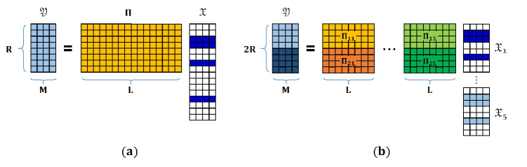
Figure 1: Joint sparsity models in $2D$. (a) General problem. (b) Elastostatic problem.

5.2.1 Signal recovery

In order to solve the joint sparsity problem (5.7), a modified version of M-SBL algorithm with structural constraint is proposed. Precisely, the general optimization problem (5.5) is modified as

$$\min_{\mathfrak{X}}\|\mathfrak{Y}-\mathbf{\Pi}\mathfrak{X}\|_{F}^{2}+\zeta\mathcal{R}_{\zeta}(\mathfrak{X})+\mathbbm{1}_{\mathcal{M}_{\rm ad}}(\mathfrak{X}),$$

where $\mathbbm{1}_{\mathcal{M}_{\rm ad}}$ denotes the indicator function of $\mathcal{M}_{\rm ad}$, i.e.,

$$\mathbbm{1}_{\mathcal{M}_{\rm ad}}({{\bf w}}):=\begin{cases}0,&{{{\bf w}}}\in\mathcal{M}_{\rm ad},\\ \infty,&\text{otherwise.}\end{cases}$$

Owing to the structural constraint on unknown density $\mathfrak{X}$, the associated structured sparsities are updated simultaneously using the constraint

$$g_{\ell}=g_{\ell+L}=\cdots=g_{\ell+d^{2}L},\quad\forall\ell=1,\cdots L.$$

The step-by-step procedure for the modified M-SBL is summarized in Algorithm 1.

Algorithm 1 Modified M-SBL for sparse signal recovery in elasticity imaging.

1:Set iterations ${\rm Iter}_{\max}\geq 1$ and threshold $1\gg\varrho>0$.

2:Set $\sigma_{\max}$ to be the largest singular value of $\mathbf{\Pi}$.

3:Set $k:=0$ and $\zeta^{(0)}:=10\times\sigma_{\max}^{2}$.

4:Set $g^{(0)}_{\ell}:=1$ for $\ell=1,2,\cdots,(d^{2}+1)L$ and $\mathbf{G}^{(0)}:={\rm diag}\left(g_{1}^{(0)},g_{2}^{(0)},\cdots,g^{(0)}_{(d^{2}+1)L}\right)$.

5:Set ${{\bm{\pi}}}_{\ell}:=\Big{(}[\mathbf{\Pi}]_{1\ell},\cdots,[\mathbf{\Pi}]_{(dR)\ell}\Big{)}^{\top}$ and ${{\bm{\pi}}}^{*}_{\ell}:=\left([\mathbf{\Pi}]^{*}_{1\ell},\cdots,[\mathbf{\Pi}]^{*}_{(dR)\ell}\right)^{\top}$.

6:for $k=1,\dots,{\rm Iter}_{\max}$ do

7:     Set $\mathbf{F}^{(k-1)}:=\left(\mathbf{\Pi}\mathbf{G}^{(k-1)}\mathbf{\Pi}^{*}+\zeta^{(k-1)}\mathbf{I}_{dR}\right)^{-1}$.

8:     Update $\mathfrak{X}^{(k)}=\mathbf{G}^{(k-1)}\mathbf{\Pi}^{*}\mathbf{F}^{(k-1)}\mathfrak{Y}$.

9:     Update: for $\ell=1,\cdots,L,$

$$g_{\ell}^{(k)}=g_{\ell+L}^{(k)}=\cdots=g_{\ell+d^{2}L}^{(k)}=\sqrt{{\displaystyle\sum_{q=1}^{d^{2}+1}\sum_{m=1}^{M}\left|\left[\mathfrak{X}_{q}^{(k)}\right]_{\ell m}\right|^{2}}\Big{/}M{\displaystyle\sum_{p=0}^{d^{2}L}{\bm{\pi}}_{\ell+p}^{*}\mathbf{F}^{(k-1)}{\bm{\pi}}_{\ell+p}}}.$$

10:     Set $\mathbf{G}^{(k)}:={\rm diag}\left(g_{1}^{(k)},g_{2}^{(k)},\cdots,g^{(k)}_{(d^{2}+1)L}\right)$.

11:     if $\displaystyle{g_{\ell}^{(k)}}/{\max_{\ell}\left(g_{\ell}^{(k)}\right)}<\varrho$ then

12:         $g_{\ell}^{(k)}=0.$

13:     end if

14:     Update $\displaystyle\zeta^{(k)}=\sqrt{{\|\mathfrak{Y}-\mathbf{\Pi}\mathfrak{X}^{(k)}\|_{F}^{2}}\Big{/}{M\,{\rm tr}\left(\mathbf{F}^{(k-1)}\right)}}$.

15:end forreturn $\hat{\mathfrak{X}}:=\mathfrak{X}^{(k)}$.

5.2.2 Preconditioning

Recall that the problem (5.6) is severely ill-posed if the inclusions are extended and not really sparse inside the background domain due to the intrinsic ill-posedness of the elasticity imaging problem. Moreover, the sensing matrix, which is associated to a physical system, has a coherence structure and its columns are not completely incoherent. This affects the performance of the sparsity based recovery algorithms. Therefore, it is desirable to introduce a surgical preconditioning procedure before executing M-SBL algorithm. For this, the singular value decomposition of the sensing matrix is considered as $\mathbf{\Pi}=\mathbf{V}\mathbf{\Sigma}\mathbf{W}^{*}$. Here $\mathbf{\Sigma}\in\mathbb{R}^{dR\times(d^{2}+1)L}$ is such that $[\mathbf{\Sigma}]_{rr}=:\sigma_{r}$, for all $r=1,\cdots,dR$, are the singular values of $\mathbf{\Pi}$ and $[\mathbf{\Sigma}]_{r\ell}=0$ for all $r\neq\ell$. The matrices $\mathbf{V}\in\mathbb{R}^{dR\times dR}$ and $\mathbf{W}\in\mathbb{R}^{(d^{2}+1)L\times(d^{2}+1)L}$ are unitary and their columns are respectively the left and right singular vectors of $\mathbf{\Pi}$. Consequently, a preconditioning weight matrix $\mathbf{P}\in\mathbb{R}^{dR\times dR}$ can be introduced as

$$\mathbf{P}=(\mathbf{\Sigma}^{2}+\theta\mathbf{I}_{dR})^{-1/2}\mathbf{V}^{*},$$

with $\theta$ being a thresholding parameter (refer, for instance, to [35, 39]). The M-SBL algorithm can then be applied to the regularized problem

$$\mathbf{P}\mathfrak{Y}=\mathbf{P}\mathbf{\Pi}\mathfrak{X}+\mathbf{P}\mathbf{E}.$$ (5.8)

5.2.3 Support identification

The application of M-SBL Algorithm 1 renders the unique minimizer $\hat{\mathfrak{X}}$ to the constraint optimization problem (5.7). Having recovered the sparse signal vector, one can identify the support set $\cup_{n=1}^{N}D_{n}$ by collecting all ${{\bf y}}_{\ell}$ such that $[\widetilde{\mathbf{X}}_{m}({{\bf y}}_{\ell})]_{q}$ is nonzero for all $q=1,\cdots,d^{2}+1$ and $m=1,\cdots,M$. In other words, it suffices to look for $\ell\in\{1,\cdots,L\}$ such that $[\hat{\mathfrak{X}}_{q}]_{\ell m}$ is non-zero for all $q=1,\cdots,d^{2}+1$ and $m=1,\cdots,M$. Towards this end, set

$$\hat{D}:=\left\{{{\bf y}}_{\ell}\;\Big{|}\;{\psi_{\ell}}\Big{/}{\displaystyle\max_{\ell\in\{1,\cdots,L\}}(\psi_{\ell})}>\xi\right\},$$ (5.9)

where $\xi$ is a pruning parameter and $\psi_{\ell}$ is defined by

$$\psi_{\ell}:=\sqrt{\sum_{q=1}^{d^{2}+1}\sum_{m=1}^{M}\left|\left[\hat{\mathfrak{X}}_{q}\right]_{\ell m}\right|^{2}},\quad 1\leq\ell\leq L.$$

Note that $\psi_{\ell}$ indicates the sparseness of the $l$-th row. Due to the numerical implementation, the values of $[\hat{\mathfrak{X}}_{q}]_{\ell m}$ cannot reach zero absolutely, though they may be very small. Consequently, this pruning step is indispensable to sweep away the values smaller than a predefined threshold depending on the noise level and numerical discretization.

5.3 Parameter reconstruction

For the quantitative evaluation of the Lamé parameters of $\hat{D}$, one needs to solve the discrete system (4.6). This can be done by formulating the constrained optimization problem

$${\rm arg}\min\limits_{\mathfrak{Z}}\,\widetilde{\zeta}\|\mathfrak{Z}\|_{1}\,\text{ subject to }\,\|\widetilde{\mathbf{Y}}-\widetilde{\mathbf{\Pi}}\mathfrak{Z}\|_{2}\leq\eta,\,\,\theta_{\min}\leq[\mathfrak{Z}]_{i}\leq\theta_{\max},\,\,i=1,\cdots,(d^{2}+1)\widetilde{L},$$ (5.10)

where $l_{1}-$ penalty is enforced in order to achieve noise robust reconstruction and the constraint

$$\theta_{\min}\leq[\mathfrak{Z}]_{i}\leq\theta_{\max},$$ (5.11)

emerges from the assumption H3. Here $\theta_{\min}$ and $\theta_{\max}$ are real numbers such that $\theta_{\min}\leq\theta_{\max}$ and $\widetilde{\zeta}$ is the constraint weight. There are several algorithms available in the literature that are tailored to solve such constrainted optimization problems and any one of them can be deployed to resolve (5.10). In this article, the C-SALSA by Afonso, Bioucas-Dias, and Figueiredo [2] is implemented. A pseudo-code implementation of C-SALSA for (5.10) is furnished in Algorithm 2. Beforehand, the sensing matrix $\widetilde{\mathbf{\Pi}}$ is normalized so that each one of its columns has a unit $l_{2}-$norm, however, the normalized matrix is still denoted by $\widetilde{\mathbf{\Pi}}$ by abuse of notation.

The idea of C-SALSA is to transform the constrained optimization problem into an unconstrained problem first. Then, the resulting problems is further transformed using a variable splitting operation before finally being resolved using Alternating Direction Method of Multipliers (ADMM). The interested readers are refered to [2] for a topical review and detailed description of C-SALSA.

Let $\mathcal{B}_{\eta}(\widetilde{\mathbf{Y}})$ be the Euclidean ball in $\mathbb{R}^{MdR}$ centered at $\widetilde{\mathbf{Y}}$ and radius $\eta$. Then, the problem (5.10) can be seen as the unconstrained problem (see [2])

$$\min_{\mathfrak{Z}}\widetilde{\zeta}\|\mathfrak{Z}\|_{1}+\mathbbm{1}_{\mathcal{B}_{\eta}(\widetilde{\mathbf{Y}})}\left(\widetilde{\mathbf{\Pi}}\mathfrak{Z}\right),$$ (5.12)

where $\mathbbm{1}_{\mathcal{B}_{\eta}(\widetilde{\mathbf{Y}})}$ is the indicator function of ${\mathcal{B}_{\eta}(\widetilde{\mathbf{Y}})}$, i.e.,

$$\mathbbm{1}_{\mathcal{B}_{\eta}(\widetilde{\mathbf{Y}})}\left({{\bf w}}\right):=\begin{cases}0,&{{\bf w}}\in{\mathcal{B}_{\eta}(\widetilde{\mathbf{Y}})},\\ \infty,&\text{otherwise}.\end{cases}$$

Let us introduce the mappings $f_{1}:\mathbb{R}^{(d^{2}+1)\widetilde{L}}\to\mathbb{R}$ and $f_{2}:\mathbb{R}^{Md\widetilde{L}}\to\mathbb{R}$ by $f_{1}({{\bf s}}):=\|{{\bf s}}\|_{1}$ and $f_{2}({{\bf s}}):=\mathbbm{1}_{\mathcal{B}_{\eta}(\widetilde{\mathbf{Y}})}({{\bf s}})$, and the corresponding Moreau proximal mappings $\Psi_{\tau f_{1}}:\mathbb{R}^{(d^{2}+1)\widetilde{L}}\to\mathbb{R}^{(d^{2}+1)\widetilde{L}}$ and $\Psi_{\tau f_{2}}:\mathbb{R}^{Md\widetilde{L}}\to\mathbb{R}^{Md\widetilde{L}}$ by

$$\Psi_{\tau f_{1}}({{\bf s}}) :={\rm arg}\min_{{{\bf v}}}\frac{1}{2}\|{{\bf v}}-{{\bf s}}\|_{2}^{2}+\tau\|{{\bf v}}\|_{1},$$

$$\Psi_{\tau f_{2}}({{\bf s}}) :={\rm arg}\min_{{{\bf w}}}\tau\mathbbm{1}_{\mathcal{B}_{\eta}(\widetilde{\mathbf{Y}})}({{\bf w}})+\frac{1}{2}\|{{\bf w}}-{{\bf s}}\|_{2}^{2}.$$

Refer, for instance, to [20] and articles cited therein for details on Moreau proximal mappings. It is worthwhile mentioning that $\Psi_{\tau f_{1}}$ with $f_{1}$ being the $l_{1}-$regularizer turns out to be simply a soft thresholding [2], i.e.,

$$\Psi_{\tau f_{1}}({{\bf s}})={\rm soft}({{\bf s}},\tau),$$

where ${\rm soft}({{\bf s}},\tau)$ reflects the component-wise operation

$$[{{\bf s}}]_{j}={\rm sign}\big{(}[{{\bf s}}]_{j}\big{)}\max\big{\{}\big{|}[{{\bf s}}]_{j}\big{|}-\tau,\;0\big{\}}.$$

In numerical implementation, the regularization parameter $\tau$ is chosen to be $\tau=0.1|\bar{\mathfrak{Z}}_{0}|$, where $|\bar{\mathfrak{Z}}_{0}|$ is the average value of $|\mathfrak{Z}|$ at the zeroth iteration in Algorithm 2. The threshold $\eta$ is fixed at $\eta=0.3\|\widetilde{\mathbf{Y}}\|_{2}$. The data fidelity parameter $\widetilde{\zeta}$ is manually selected as the optimal choice from the set $\{8,4,2,1,1/2,1/4,1/8\}$. The parameters $\theta_{\min}$ and $\theta_{\max}$ in (5.11) are set to $-\infty$ and $+\infty$, respectively. Even in this (unconstrained) setup, the constraint in (5.11) is necessary to introduce additional variable splitting, which allows much faster convergence. This type of additional splitting is quite often used in ADMM. Finally, the relative change of the cost function in (5.10) is used as a stopping criterion, i.e., the algorithm is executed until $\left|\left(C_{k}-C_{k-1}\right)/C_{k}\right|<10^{-4}$ is satisfied, where $C_{k}$ is the cost function at the $k$-th iteration. With these choices of parameters, the relevant pseudo-code implementation of C-SALSA for the resolution of the unconstrained problem (5.12) is provided in Algorithm 2.

Algorithm 2 C-SALSA for parameter recovery in elasticity imaging.

1:Set $k=0$, choose $\tau>0$.

2:Set ${\bf a}_{0}^{(i)}={\bf b}_{0}^{(i)}=0$, for $i=1,2$.

3:repeat

4:     $\mathbf{r}_{k}=\widetilde{\zeta}({\bf a}_{k}^{(1)}+{\bf b}_{k}^{(1)})+\widetilde{\mathbf{\Pi}}^{*}({\bf a}_{k}^{(2)}+{\bf b}_{k}^{(2)})$.

5:     $\mathfrak{Z}_{k+1}=\left[(1+{\widetilde{\zeta}}^{2})\mathbf{I}+\widetilde{\mathbf{\Pi}}^{*}\widetilde{\mathbf{\Pi}}\right]^{-1}\mathbf{r}_{k}$.

6:     ${\bf a}_{k+1}^{(1)}=\Psi_{\tau f_{1}}(\widetilde{\zeta}\mathfrak{Z}_{k+1}-{\bf b}_{k}^{(1)})$.

7:     ${\bf a}_{k+1}^{(2)}=\Psi_{f_{2}}(\widetilde{\mathbf{\Pi}}\mathfrak{Z}_{k+1}-{\bf b}_{k}^{(2)})$.

8:     ${\bf b}_{k+1}^{(1)}={\bf b}_{k}^{(1)}-\widetilde{\zeta}\mathfrak{Z}_{k+1}+{\bf a}_{k+1}^{(i)}$.

9:     ${\bf b}_{k+1}^{(2)}={\bf b}_{k}^{(2)}-\widetilde{\mathbf{\Pi}}\mathfrak{Z}_{k+1}+{\bf a}_{k+1}^{(i)}$.

10:     $k\longleftarrow k+1$.

11:until Stopping criterion is satisfied.

6 Numerical validation of reconstruction scheme

In this section, some numerical experiments are performed in order to validate the proposed reconstruction scheme. Let us first provide the details of the numerical scheme for the forward model in Section 6.1. The examples of the reconstruction of different inclusions are furnished in Section 6.2.

6.1 Forward solver

In order to solve the forward problem for data acquisition, the boundary layer potential technique is used together with the so-called Nyström discretization scheme. Let us briefly fix the ideas about the resolution of the forward problem. For simplicity, a two- dimensional case is considered. Note that the vector space $\Psi$ in two-dimensions is given by

$$\Psi={\rm Span}\left\{\begin{pmatrix}1\\ 0\end{pmatrix},\begin{pmatrix}0\\ 1\end{pmatrix},\begin{pmatrix}x_{2}\\ -x_{1}\end{pmatrix}\right\}.$$

For $M$ distinct points ${{\bf z}}_{1},\cdots,{{\bf z}}_{M}\in\mathbb{R}^{2}\setminus\overline{\Omega}$, generate

$$\mathbf{U}_{m}({{\bf x}})=\mathbf{\Gamma}({{\bf x}}-{{\bf z}}_{m})\cdot\begin{pmatrix}1\\ 0\end{pmatrix}+\alpha_{1}\begin{pmatrix}1\\ 0\end{pmatrix}+\alpha_{2}\begin{pmatrix}0\\ 1\end{pmatrix}+\alpha_{3}\begin{pmatrix}x_{2}\\ -x_{1}\end{pmatrix},$$ (6.1)

where $\alpha_{1},\alpha_{2},\alpha_{3}\in\mathbb{R}$ are chosen in such a way that $\mathbf{U}_{m}|_{\partial\Omega}\in L^{2}_{\Psi}(\partial\Omega)$, i.e.,

$$\int_{\partial\Omega}\mathbf{U}_{m}\cdot\begin{pmatrix}1\\ 0\end{pmatrix}d\sigma=\int_{\partial\Omega}\mathbf{U}_{m}\cdot\begin{pmatrix}0\\ 1\end{pmatrix}d\sigma=\int_{\partial\Omega}\mathbf{U}_{m}\cdot\begin{pmatrix}x_{2}\\ -x_{1}\end{pmatrix}d\sigma=0.$$

The surface traction $\mathbf{g}_{m}$, $m=1,\cdots,M$, is then calculated by the relation $\mathbf{g}_{m}={\partial\mathbf{U}_{m}}/{\partial\bm{\nu}}|_{\partial\Omega}$. Remark that $\mathcal{L}_{\lambda_{0},\mu_{0}}[\mathbf{U}_{m}]=0$ in $\Omega$ and consequently $\mathbf{g}_{m}\in L^{2}_{\Psi}(\partial\Omega)$.

In order to generate the displacement field ${{\bf u}}_{m}$ in the presence of inclusions, $D_{1},\cdots,D_{N}$, the transmission problem (2.3) is solved using a layer potential technique. Towards this end, the single layer potential associated to the linear elasticity operator $\mathcal{L}_{\lambda_{0},\mu_{0}}$ is defined by

$$\mathcal{S}_{\Omega}[{\bm{\varphi}}]({{\bf x}}):=\int_{\partial\Omega}\mathbf{\Gamma}({{\bf x}}-{{\bf y}})\cdot{\bm{\varphi}}({{\bf y}})d\sigma({{\bf y}}),\qquad{{\bf x}}\in\mathbb{R}^{2},\quad{\bm{\varphi}}\in L^{2}(\partial\Omega)^{2}.$$

It is well known (see, for instance, [23]) that $\mathcal{S}_{\Omega}[{\bm{\varphi}}]$ satisfies the jump relations

$$\frac{\partial}{\partial\bm{\nu}}\mathcal{S}_{\Omega}[{\bm{\varphi}}]\Big{|}_{\pm}({{\bf x}})=\left(\pm\frac{1}{2}\mathcal{I}+\mathcal{K}^{*}_{\Omega}\right){\bm{\varphi}}({{\bf x}}),\qquad{\rm a.e.}\quad{{\bf x}}\in\partial\Omega,$$

where $\mathcal{K}^{*}_{\Omega}$ is the $L^{2}-$adjoint operator of $\mathcal{K}_{\Omega}$ and is defined by

$$\mathcal{K}^{*}_{\Omega}[{\bm{\varphi}}]({{\bf x}}):={\rm p.v.}\displaystyle\int_{\partial\Omega}\frac{\partial}{\partial\bm{\nu}_{{\bf x}}}\mathbf{\Gamma}({{\bf x}}-{{\bf y}})\cdot{\bm{\varphi}}({{\bf y}})d\sigma({{\bf y}}),\quad{\rm a.e.}\qquad\,{{\bf x}}\in\partial\Omega,\quad{\bm{\varphi}}\in L^{2}(\partial\Omega)^{2}.$$

Then, the solution to the system(2.3) can be represented as (see, e.g., [8, Theorem 6.15])

$${{\bf u}}_{m}({{\bf x}})=\begin{cases}\mathcal{S}_{\Omega}[\bm{\eta}_{m}]+\mathcal{S}_{D}[{\bm{\psi}}_{m}]({{\bf x}}),&\mbox{if }{{\bf x}}\in\Omega\setminus\overline{D},\\ \widetilde{\mathcal{S}}_{D}[{\bm{\varphi}}_{m}]({{\bf x}}),&{{\bf x}}\in D,\end{cases}$$ (6.2)

where $({\bm{\varphi}}_{m},{\bm{\psi}}_{m},\bm{\eta}_{m})\in L^{2}(\partial D)^{2}\times L^{2}_{\Psi}(\partial\Omega)^{2}\times L^{2}(\partial D)^{2}$ is the unique solution to

$$\begin{bmatrix}\displaystyle\displaystyle\widetilde{\mathcal{S}}_{D}|_{\partial\mathcal{D}}&\displaystyle-\mathcal{S}_{D}|_{\partial\mathcal{D}}&\displaystyle-\mathcal{S}_{\Omega}|_{\partial\mathcal{D}}\\ \displaystyle\left(-\frac{1}{2}\mathcal{I}+\widetilde{\mathcal{K}}^{*}_{D}\right)&-\displaystyle\left(\frac{1}{2}\mathcal{I}+\mathcal{K}^{*}_{D}\right)&-\displaystyle\frac{\partial}{\partial\bm{\nu}}\mathcal{S}_{\Omega}|_{\partial D}\\ \displaystyle 0&\displaystyle\frac{\partial}{\partial\bm{\nu}}\mathcal{S}_{D}|_{\partial\Omega}&\displaystyle\left(-\frac{1}{2}\mathcal{I}+\mathcal{K}_{\Omega}^{*}\right)\end{bmatrix}\begin{bmatrix}{\bm{\varphi}}_{m}\\ {\bm{\psi}}_{m}\\ \bm{\eta}_{m}\end{bmatrix}=\begin{bmatrix}0\\ 0\\ \mathbf{g}_{m}\end{bmatrix},$$ (6.3)

subject to the constraint ${{\bf u}}_{m}\in L^{2}_{\Psi}(\partial\Omega)$, thanks to the transmission and the boundary conditions. Here $\widetilde{\mathcal{S}}_{D}$ and $\widetilde{\mathcal{K}}_{D}^{*}$ are the operators related to the interior parameters $(\lambda,\mu)$.

The aim here is to solve the system (6.3) for $({\bm{\varphi}}_{m},{\bm{\psi}}_{m},\bm{\eta}_{m})$ and then evaluate ${{\bf u}}_{m}|_{\partial\Omega}$ using representation (6.2). In order to numerically solve system (6.3), express $\mathcal{K}^{*}_{\Omega}$ as

$$\mathcal{K}^{*}_{\Omega}[\mathbf{f}]({{\bf x}})={\rm p.v.}\int_{0}^{1}\frac{\partial}{\partial\bm{\nu}_{{{\bf x}}}}\mathbf{\Gamma}({{\bf x}}-{{\bf x}}(t))\cdot\mathbf{f}({{\bf x}}(t))|{{\bf x}}^{\prime}(t)|dt,\quad\,{{\bf x}}\in\partial D,$$ (6.4)

where ${{\bf x}}(t)$ is a parametrization of $\partial\Omega$. Then the Nyström discretization, with $P$ boundary points $\{{{\bf x}}_{p}\}_{p=1}^{P}$ and weights $w_{p}$, renders

$$\mathcal{K}^{*}_{\Omega}[\mathbf{f}]({{\bf x}})\approx\sum_{p=1}^{P}\frac{\partial}{\partial\bm{\nu}_{{\bf x}}}\mathbf{\Gamma}({{\bf x}}-{{\bf x}}_{p})\cdot\mathbf{f}_{p}|{{\bf x}}^{\prime}_{p}|w_{p},\quad\,{{\bf x}}\in\partial\Omega,$$ (6.5)

where $\mathbf{f}_{p}=\mathbf{f}({{\bf x}}_{p})$ for $p=1,\cdots,P$. Here, the simplest quadrature rule

$$\int_{0}^{1}\mathbf{f}(t)dt\approx\sum_{p=1}^{P}\frac{1}{P}\mathbf{f}\left(\frac{p}{P}\right),$$

is used. It is emphasized that the integral (6.4) is defined as the Cauchy principal value. Thus, the singularity of ${\partial}[\mathbf{\Gamma}({{\bf x}}-{{\bf x}}_{p})]/{\partial\bm{\nu}_{{\bf x}}}$ at ${{\bf x}}={{\bf x}}_{p}$ should be evaluated in the sense of the Cauchy principle value. The numerical computation of $\mathcal{K}^{*}_{\Omega}$ can be realized using (6.5). Similarly, $\mathcal{K}_{\Omega}$, $\mathcal{S}_{\Omega}$ and $\mathcal{D}_{\Omega}$ can be descretized as

$$\mathcal{K}_{\Omega}[\mathbf{f}]({{\bf x}}) \approx\sum_{p=1}^{P}\frac{\partial}{\partial\bm{\nu}({{\bf x}}_{p})}\mathbf{\Gamma}({{\bf x}}-{{\bf x}}_{p})\cdot\mathbf{f}_{p}|{{\bf x}}^{\prime}_{p}|w_{p},\quad\,{{\bf x}}\in\partial\Omega,$$

$$\mathcal{S}_{\Omega}[\mathbf{f}]({{\bf x}}) \approx\sum_{p=1}^{P}\mathbf{\Gamma}({{\bf x}}-{{\bf x}}_{p})\cdot\mathbf{f}_{p}|{{\bf x}}^{\prime}_{p}|w_{p},\quad{{\bf x}}\in\Omega,$$

$$\mathcal{D}_{\Omega}[\mathbf{f}]({{\bf x}}) \approx\sum_{p=1}^{P}\frac{\partial}{\partial\bm{\nu}({{\bf x}}_{p})}\mathbf{\Gamma}({{\bf x}}-{{\bf x}}_{p})\cdot\mathbf{f}_{p}|{{\bf x}}^{\prime}_{p}|w_{p},\quad{{\bf x}}\in\Omega.$$

Consequently, the integral system (6.3) can be discretized and solved for $({\bm{\varphi}}_{m},{\bm{\psi}}_{m},\bm{\eta}_{m})$. If only sparsely sampled data $({{\bf u}}_{m}-\mathbf{U}_{m})$ are available, the preprocessing of the data $({{\bf u}}_{m}-\mathbf{U}_{m})$ using the Calerón preconditioner $(-\mathcal{I}/2+\mathcal{K}_{\Omega})$ can be done in the similar fashion after being interpolated to dense samples as discussed in Section 4.3.1.

6.2 Numerical experiments

For numerical examples, let the background domain $\Omega$ to be an ellipse of semi-major and semi-minor axes $10mm$ and $7mm$ respectively with shear and compression moduli $\mu_{0}=\lambda_{0}=1GPa$. Three different kinds of inclusions are considered for numerical experiments. Precisely, the examples of sparse, extended and thin or worm-like inclusions are taken into account. The sparse inclusions are modeled with three unit disks. The extended inclusion is modeled with a non-convex kite shaped domain with the size comparable to that of the background domain in order of magnitude. By thin or worm-like inclusions, it is meant that one dimension of the inclusions is much smaller than the other dimension. The examples of straight and curved thin inclusions are dealt with. The test geometries are delineated in Figure 2. The field of view is discretized to have a grid size $1/3mm$ for all reconstructions. The Lamé parameters of the three inclusions in the sparse case are both fixed at $7GPa$ for the leftmost inclusion, $2GPa$ for the inclusion in the middle, and $2.5GPa$ for the rightmost inclusion. For the rest of the examples, the Lamé parameters of the targets are both fixed at $2GPa$.

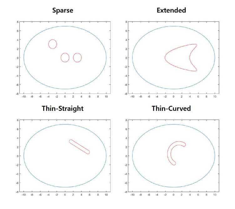
Figure 2: Geometric configuration and different test inclusions.

6.2.1 Parameter selection

For all experiments, four measurement sets are used, i.e., $M=4$. Accordingly, points ${{\bf z}}_{1}=(12,11)$, ${{\bf z}}_{2}=(9,-11)$, ${{\bf z}}_{3}=(-1,8)$ and ${{\bf z}}_{4}=(-50,0)$ are used in (6.1) to define $\{\mathbf{U}_{m}\}_{m=1}^{4}$ and $\{\mathbf{g}_{m}\}_{m=1}^{4}$. The forward data is acquired using the numerical scheme described in Section 6.1. $P=2000$ discretization points on $\partial\Omega$ and $\partial D_{n}$, for each $n$, are used for the example of sparse inclusions, and $P=5000$ points are used for rest of the examples. Three different sets of the uniformly distributed full view measurement points $\{{{\bf x}}_{r}\}_{r=1}^{R}$ with $R=100$, $32$, $16$ and a set of limited view (with angle $3\pi/2$) measurement points on $\partial\Omega$ with $R=16$ are taken into account. The latter case is indicated hereinafter by $R=16p$. The measurement setups are depicted in Figure 3. An additive Gaussian noise with signal-to-noise ratio $40dB$ was added to the boundary measurement vectors $({{\bf u}}_{m}-\mathbf{U}_{m})\big{|}_{\partial\Omega}$ for all simulations.

Figure 3: Configuration of the measurement points on the boundary of $\Omega$. (a) $R=100$. (b) $R=32$. (c) $R=16$. (d) $R=16p$.

In order to recover the density $\mathfrak{X}$ over the support $\hat{D}$, the modified M-SBL Algorithm 1 is applied on the preconditioned problem (5.8) using regularization parameter $\theta=10^{-2}\times\sigma_{\max}^{2}$, where $\sigma_{\max}$ denotes the maximum singular value of the sensing matrix $\Pi$. The threshold parameter $\varrho$ in Algorithm 1 is set to be $\varrho=10^{-3}$.

For support identification, the pruning parameter $\xi$ in (5.9) is set to be $\xi=0$, i.e., small values are not pruned out and the obtained information is fully utilized in order to avoid a sub-optimal selection of $\xi$. The box constraint parameters $\theta_{\min}$ and $\theta_{\max}$ in (5.11) are set to be very large so that $[\mathfrak{Z}]_{i}$ can simply assume values in $(-\infty,+\infty)$.

The selected optimal values of the parameters for Algorithms 1 and 2 are summarized in Table  1. These parameters are used for all examples except for data fidelity parameter $\widetilde{\zeta}$, which is gradually decreased in value with respect to the decrease in the number of measurement points.

Table 1: Parameters choices for numerical simulations.

Proposed Method Sparse target Thin-Straight target Thin-Curved target Extended target Step 1: M-SBL $\mbox{Iter}_{\max}=50$ $\mbox{Iter}_{\max}=50$ $\mbox{Iter}_{\max}=50$ $\mbox{Iter}_{\max}=50$ with preconditioning with preconditioning with preconditioning with preconditioning Step 2: C-SALSA $\tau=0.1|\bar{\mathfrak{Z}}_{0}|$ $\tau=0.1|\bar{\mathfrak{Z}}_{0}|$ $\tau=0.1|\bar{\mathfrak{Z}}_{0}|$ $\tau=0.1|\bar{\mathfrak{Z}}_{0}|$ $\eta=0.3\|\widetilde{\mathbf{Y}}\|_{2}$ $\eta=0.3\|\widetilde{\mathbf{Y}}\|_{2}$ $\eta=0.3\|\widetilde{\mathbf{Y}}\|_{2}$ $\eta=0.3\|\widetilde{\mathbf{Y}}\|_{2}$ $\widetilde{\zeta}=2\leavevmode\nobreak\ (R=100)$ $\widetilde{\zeta}=4\leavevmode\nobreak\ (R=100)$ $\widetilde{\zeta}=4\leavevmode\nobreak\ (R=100)$ $\widetilde{\zeta}=8\leavevmode\nobreak\ (R=100)$ $\widetilde{\zeta}=1/2\leavevmode\nobreak\ (R=32)$ $\widetilde{\zeta}=2\leavevmode\nobreak\ (R=32)$ $\widetilde{\zeta}=1\leavevmode\nobreak\ (R=32)$ $\widetilde{\zeta}=4\leavevmode\nobreak\ (R=32)$ $\widetilde{\zeta}=1/4\leavevmode\nobreak\ (R=16)$ $\widetilde{\zeta}=1\leavevmode\nobreak\ (R=16)$ $\widetilde{\zeta}=1/2\leavevmode\nobreak\ (R=16)$ $\widetilde{\zeta}=2\leavevmode\nobreak\ (R=16)$ $\widetilde{\zeta}=1/4\leavevmode\nobreak\ (R=16p)$ $\widetilde{\zeta}=1/2\leavevmode\nobreak\ (R=16p)$ $\widetilde{\zeta}=1/2\leavevmode\nobreak\ (R=16p)$ $\widetilde{\zeta}=2\leavevmode\nobreak\ (R=16p)$  

6.2.2 Simulation results

The reconstructed shear and compression moduli for different inclusions together with estimated support of the inclusions are provided in Figures 4–7 for sparse, thin straight, thin curved and extended inclusions respectively. For all the listed inclusions, the results are furnished with different configurations of measurement points (with $R=100$, $32$, $16$, $16p$) as precised earlier. When $R=100$, the proposed algorithm clearly recovered the structures of the inclusions and their constitutive parameters in all cases. For instance, for sparse inclusions, even though the parameter values have been varied by tuning the optimization parameters, their relative relationships remained the same so that the leftmost inclusion always appears to have the highest value and the middle one has the lowest value (see Figure 4). It is observed that the overall reconstruction performance gradually suffers when the number of measurement points decreases. Nevertheless, the results corresponding to $R=32$ are comparable to those of $R=100$. Even when $R=16$, the simulations are mostly able to indicate the crude shapes of the inclusions.

However, when the measurement points only cover the partial aperture ($R=16p$ and $3\pi/2$ angle of view), the results are distorted. The reconstructions for thin and extended targets show comparatively less accurate results than those for the sparse targets. It is worthwhile to mention that M-SBL was still able to localize the anomalies even in the deteriorated conditions. In the deteriorated cases from the partial aperture, although the M-SBL algorithm recovered the locations outside the expected regions, the estimated M-SBL values are relatively higher inside and near the boundary of the inclusions than spurious detected regions outside the inclusions (see Figure 8). The points outside the inclusions with small values can be easily filtered by appropriately tuning the pruning parameter $\xi$.

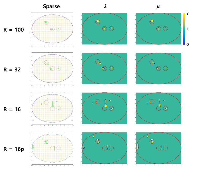
Figure 4: Reconstruction of multiple disk-like inclusions. Left to Right: $\hat{D}$, $\lambda$, and $\mu$.

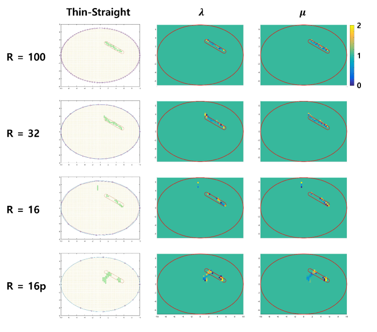
Figure 5: Reconstruction of a thin-straight inclusion. Left to Right: $\hat{D}$, $\lambda$, and $\mu$.

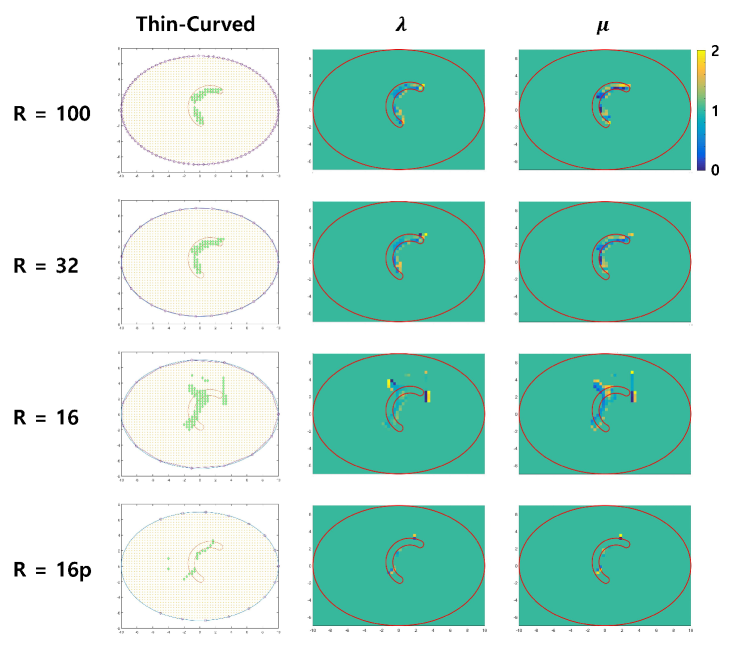
Figure 6: Reconstruction of a thin-curved inclusion. Left to Right: $\hat{D}$, $\lambda$, and $\mu$.

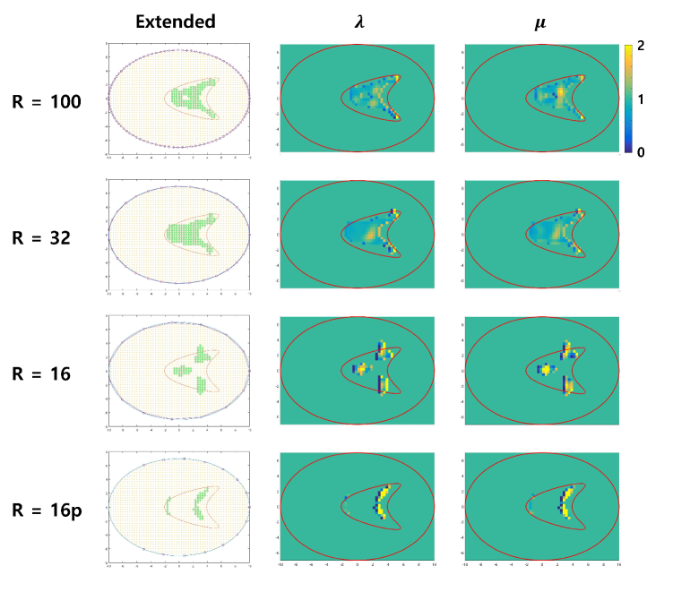
Figure 7: Reconstruction of an extended inclusion. Left to Right: $\hat{D}$, $\lambda$, and $\mu$.

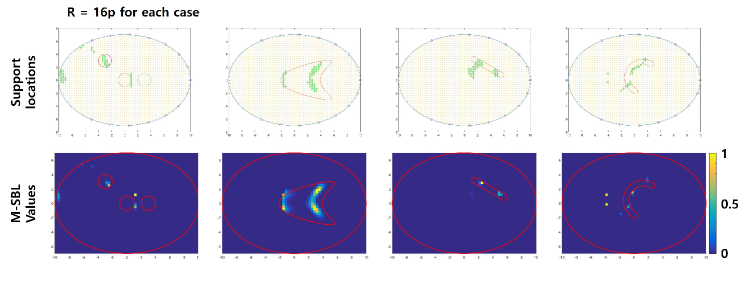
Figure 8: Support identification using M-SBL in deteriorated cases. Top: Reconstructed support sets. Bottom: The normalized M-SBL values $\psi_{\ell}/\max_{i\in\{1,\cdots,L\}}(\psi_{i})$.

7 Conclusion

A joint sparse recovery based direct algorithm was proposed to reconstruct the spatial support of multiple elastic inclusions and their material parameters using only a few measurements of the displacement over a very coarse grid of boundary points (in the sense of Nyquist sampling rate). The inverse problem for support detection was converted to a joint sparse recovery problem for internal data (linked to the displacement and strain fields inside the support set of the inclusions) by virtue of an integral formulation. The sparse signal recovery problem resulting therefrom was resolved for an exact and unique solution by invoking a modified M-SBL algorithm with structural constraints. Then, using the leverage of the learned internal information about the displacement field, a linear inverse problem for quantitative evaluation of material parameters was formulated. The resulting problem was then converted to a noise robust constraint optimization problem, which was subsequently solved using the C-SALSA. The proposed imaging algorithm was computationally very efficient and was felicitous to demonstrate very accurate reconstruction since it is non-iterative and does not require any linearization or computations of multiple forward solutions. The advantage is taken here of the learned internal data and the sparsity of the support set of the inclusions inside the elastic medium to reduce the mathematical ill-posedness of the underlying inverse problem. In fact, the recovery of such an information is very novel and pertinent. This additional information compensates for the under-determined data and therefore renders stability to the reconstruction framework. In addition, since no linearization or simplifying approximations are used, the proposed technique provides reconstruction with better resolution and quality than classical techniques. However, a more sophisticated quantitative mathematical analysis is certainly necessary in order to ascertain the stability and resolution properties of the proposed framework in terms of the relative size of the inclusion, the number of measurement fields, the number and the placement of the measurement points on the boundary, and the aperture size. This will be the subject of future investigations. Albeit, the elastostatic problem is undertaken in this article, the quasi-static or time-harmonic elasticity problems are also amenable to the same treatment with minor changes. Moreover, the elasticity imaging problem in the so-called quasi-incompressible regime can also be dealt with and will be investigated in future.

Appendix A Evaluation of integral kernals

Let us provide the explicit expressions for different kernels involved in our integral formulation and those required to compute the sensing matrix of the reconstruction framework. For brevity, only the two dimensional case is entertained.

Following identities will be handy in ensuing calculations. For all $i,j\in\{1,2\}$ and ${{\bf x}},{{\bf y}}\in\mathbb{R}^{2}$, such that ${{\bf x}}\neq{{\bf y}}$,

$$\begin{cases}\displaystyle\frac{\partial}{\partial y_{i}}\ln|{{\bf x}}-{{\bf y}}|=-\frac{x_{i}-y_{i}}{|{{\bf x}}-{{\bf y}}|^{2}},\\ \displaystyle\frac{\partial^{2}}{\partial y_{i}\partial y_{j}}\ln|{{\bf x}}-{{\bf y}}|=-2\frac{(x_{i}-y_{i})(x_{j}-y_{j})}{|{{\bf x}}-{{\bf y}}|^{4}}+\delta_{ij}\frac{1}{|{{\bf x}}-{{\bf y}}|^{2}},\\ \displaystyle\Delta_{{\bf y}}\ln|{{\bf x}}-{{\bf y}}|=0.\end{cases}$$ (A.1)

A.1 Surface traction of Kelvin matrix and boundary integral operators

Recall from [9, Appendix A] that, for all ${{\bf x}},{{\bf y}}\in\mathbb{R}^{2}$, ${{\bf x}}\neq{{\bf y}}$ and $i,j\in\{1,2\}$,

$$\left(\frac{\partial\mathbf{\Gamma}}{\partial\bm{\nu}_{{\bf y}}}({{\bf x}},{{\bf y}})\right)_{ij}= \left[a\delta_{ij}+b\frac{(x_{i}-y_{i})(x_{j}-y_{j})}{|{{\bf x}}-{{\bf y}}|^{2}}\right]\left(\sum_{k=1}^{2}\frac{\nu_{k}(x_{k}-y_{k})}{|{{\bf x}}-{{\bf y}}|^{2}}\right)$$

$$-a\frac{\nu_{j}(x_{i}-y_{i})-\nu_{i}(x_{j}-y_{j})}{|{{\bf x}}-{{\bf y}}|^{2}},$$ (A.2)

$$\nu_{i}= [\bm{\nu}]_{i},\quad a:=-\frac{\mu_{0}}{2\pi(\lambda_{0}+2\mu_{0})},\quad\text{and}\quad b:=-\frac{\lambda_{0}+\mu_{0}}{\pi(\lambda_{0}+2\mu_{0})}.$$ (A.3)

Therefore, thanks to (A.2), operators $\mathcal{S}_{\Omega}$, $\mathcal{D}_{\Omega}$ and $\mathcal{K}_{\Omega}$ can be evaluated as

$$\mathcal{S}_{\Omega}[{\bm{\varphi}}]({{\bf x}}):=\displaystyle\left(\sum_{i,j=1}^{2}\int_{\partial\Omega}\left[\mathbf{\Gamma}({{\bf x}}-{{\bf y}})\right]_{ij}\cdot\left[{\bm{\varphi}}({{\bf y}})\right]_{j}d\sigma({{\bf y}})\right)\mathbf{e}_{i},\quad\,{{\bf x}}\in\mathbb{R}^{2}\setminus\partial\Omega,$$

$$\mathcal{D}_{\Omega}[{\bm{\varphi}}]({{\bf x}}):=\displaystyle\left(\sum_{i,j=1}^{2}\int_{\partial\Omega}\left[\frac{\partial}{\partial\bm{\nu}_{{\bf y}}}\mathbf{\Gamma}({{\bf x}}-{{\bf y}})\right]_{ij}\cdot\left[{\bm{\varphi}}({{\bf y}})\right]_{j}d\sigma({{\bf y}})\right)\mathbf{e}_{i},\quad\,{{\bf x}}\in\mathbb{R}^{2},$$

$$\mathcal{K}_{\Omega}[{\bm{\varphi}}]({{\bf x}}):=\displaystyle\left(\sum_{i,j=1}^{2}{\rm p.v.}\int_{\partial\Omega}\left[\frac{\partial}{\partial\bm{\nu}_{{\bf y}}}\mathbf{\Gamma}({{\bf x}}-{{\bf y}})\right]_{ij}\cdot\left[{\bm{\varphi}}({{\bf y}})\right]_{j}d\sigma({{\bf y}})\right)\mathbf{e}_{i},\quad{\rm a.e.}\quad\,{{\bf x}}\in\partial\Omega,$$

for all ${\bm{\varphi}}\in L^{2}_{\Psi}(\partial\Omega)$.

A.2 Divergence of Kelvin matrix

It is reminded that (see, e.g., [3, Lemma 3.3.2])

$$\nabla_{{\bf y}}\cdot\mathbf{\Gamma}({{\bf x}},{{\bf y}})=\frac{1}{(\lambda_{0}+2\mu_{0})}\nabla_{{\bf y}}\Phi({{\bf x}},{{\bf y}})=\frac{1}{(\lambda_{0}+2\mu_{0})}\sum_{i=1}^{2}\frac{\partial}{\partial y_{i}}\Phi({{\bf x}},{{\bf y}})\mathbf{e}_{i},$$ (A.4)

where $\Phi({{\bf x}},\cdot):\mathbb{R}^{2}\to\mathbb{R}$, for fixed ${{\bf x}}\in\mathbb{R}^{2}$, is the fundamental solution to the Laplace equation in $\mathbb{R}^{2}$, that is, $\Delta_{{\bf y}}\Phi({{\bf x}},{{\bf y}})=\delta_{{\bf x}}({{\bf y}})$, for all ${{\bf x}},{{\bf y}}\in\mathbb{R}^{2}$ and is given by

$$\Phi({{\bf x}},{{\bf y}})=\displaystyle\frac{1}{2\pi}\ln|{{\bf x}}-{{\bf y}}|,\quad\forall{{\bf x}},{{\bf y}}\in\mathbb{R}^{2},\quad{{\bf x}}\neq{{\bf y}}.$$

After fairly easy manipulations and using identities (A.1) in (A.4), one arrives at

$$\nabla_{{\bf y}}\cdot\mathbf{\Gamma}({{\bf x}},{{\bf y}})=\frac{a}{\mu_{0}}\sum_{i=1}^{2}\frac{(x_{i}-y_{i})}{|{{\bf x}}-{{\bf y}}|^{2}}\mathbf{e}_{i},\quad{{\bf x}},{{\bf y}}\in\mathbb{R}^{2},\quad{{\bf x}}\neq{{\bf y}}.$$

A.3 Strain of Kelvin matrix

In order to calculate $\Big{[}\mathcal{E}[\mathbf{\Gamma}({{\bf x}},\cdot)]({{\bf y}})\Big{]}_{ijk}$, express $\mathbf{\Gamma}$ as

$$\gamma_{ij}({{\bf x}}-{{\bf y}})=\alpha\delta_{ij}\ln|{{\bf x}}-{{\bf y}}|+\beta(x_{i}-y_{i})\frac{\partial}{\partial y_{j}}\ln|{{\bf x}}-{{\bf y}}|,\quad{{\bf x}},{{\bf y}}\in\mathbb{R}^{2},\quad{{\bf x}}\neq{{\bf y}},$$

where $\alpha$ and $\beta$ are given by (3.2). Therefore,

$$\frac{\partial}{\partial y_{k}}\gamma_{ij}({{\bf x}}-{{\bf y}})$$

$$= \phantom{-1}\alpha\delta_{ij}\frac{\partial}{\partial y_{k}}\ln|{{\bf x}}-{{\bf y}}|+\beta\frac{\partial}{\partial y_{k}}(x_{i}-y_{i})\frac{\partial}{\partial y_{j}}\ln|{{\bf x}}-{{\bf y}}|+\beta(x_{i}-y_{i})\frac{\partial^{2}}{\partial y_{k}\partial y_{j}}\ln|{{\bf x}}-{{\bf y}}|$$

$$= -\alpha\delta_{ij}\frac{(x_{k}-y_{k})}{|{{\bf x}}-{{\bf y}}|^{2}}+\beta\delta_{ik}\frac{(x_{j}-y_{j})}{|{{\bf x}}-{{\bf y}}|^{2}}+\beta\delta_{jk}\frac{(x_{i}-y_{i})}{|{{\bf x}}-{{\bf y}}|^{2}}-2\beta\frac{(x_{i}-y_{i})(x_{j}-y_{j})(x_{k}-y_{k})}{|{{\bf x}}-{{\bf y}}|^{4}}.$$

Consequently, $\Big{[}\mathcal{E}[\mathbf{\Gamma}({{\bf x}},\cdot)]({{\bf y}})\Big{]}_{ijk}$ can be calculate, for all $i,j,k\in\{1,2\}$, as

$$2\Big{[}\mathcal{E}[\mathbf{\Gamma}({{\bf x}},\cdot)]({{\bf y}})\Big{]}_{ijk}=\left(\frac{\partial\gamma_{ij}}{\partial y_{k}}({{\bf x}},{{\bf y}})+\frac{\partial\gamma_{ik}}{\partial y_{j}}({{\bf x}},{{\bf y}})\right)$$

$$= -\alpha\delta_{ij}\frac{(x_{k}-y_{k})}{|{{\bf x}}-{{\bf y}}|^{2}}+\beta\delta_{ik}\frac{(x_{j}-y_{j})}{|{{\bf x}}-{{\bf y}}|^{2}}+\beta\delta_{jk}\frac{(x_{i}-y_{i})}{|{{\bf x}}-{{\bf y}}|^{2}}-2\beta\frac{(x_{i}-y_{i})(x_{j}-y_{j})(x_{k}-y_{k})}{|{{\bf x}}-{{\bf y}}|^{4}}$$

$$-\alpha\delta_{ik}\frac{(x_{j}-y_{j})}{|{{\bf x}}-{{\bf y}}|^{2}}+\beta\delta_{ij}\frac{(x_{k}-y_{k})}{|{{\bf x}}-{{\bf y}}|^{2}}+\beta\delta_{jk}\frac{(x_{i}-y_{i})}{|{{\bf x}}-{{\bf y}}|^{2}}-2\beta\frac{(x_{i}-y_{i})(x_{j}-y_{j})(x_{k}-y_{k})}{|{{\bf x}}-{{\bf y}}|^{4}}$$

$$= \left(\beta-\alpha\right)\left[\delta_{ij}\frac{(x_{k}-y_{k})}{|{{\bf x}}-{{\bf y}}|^{2}}+\delta_{ik}\frac{(x_{j}-y_{j})}{|{{\bf x}}-{{\bf y}}|^{2}}\right]+2\beta\delta_{jk}\frac{(x_{i}-y_{i})}{|{{\bf x}}-{{\bf y}}|^{2}}-4\beta\frac{(x_{i}-y_{i})(x_{j}-y_{j})(x_{k}-y_{k})}{|{{\bf x}}-{{\bf y}}|^{4}}.$$

Finally, by remarking that $a=\beta-\alpha$, one arrives at

$$\Big{[}\mathcal{E}[\mathbf{\Gamma}({{\bf x}},\cdot)]({{\bf y}})\Big{]}_{ijk}= \frac{a}{2}\left[\delta_{ij}\frac{(x_{k}-y_{k})}{|{{\bf x}}-{{\bf y}}|^{2}}+\delta_{ik}\frac{(x_{j}-y_{j})}{|{{\bf x}}-{{\bf y}}|^{2}}\right]+\beta\delta_{jk}\frac{(x_{i}-y_{i})}{|{{\bf x}}-{{\bf y}}|^{2}}$$

$$-2\beta\frac{(x_{i}-y_{i})(x_{j}-y_{j})(x_{k}-y_{k})}{|{{\bf x}}-{{\bf y}}|^{4}}.$$

References

- [1] T. Abbas, H. Ammari, G. Hu, A. Wahab, and J. C. Ye, Two-dimensional elastic scattering coefficients and enhancement of nearly elastic cloaking, J. Elast., DOI: 10.1007/s10659-017-9624-7.
- [2] M. Afonso, J. Bioucas-Dias, and M. Figueiredo, An augmented Lagrangian approach to the constrained optimization formulation of imaging inverse problems, IEEE Trans. Image Process., 20 (2011), pp. 681–695.
- [3] H. Ammari, An Introduction to Mathematics of Emerging Biomedical Imaging, Math. Appl. (Berlin) 62, Springer-Verlag, Berlin, 2008.
- [4] H. Ammari, E. Bretin, J. Garnier, W. Jing, H. Kang, and A. Wahab, Localization, stability, and resolution of topological derivative based imaging functionals in elasticity, SIAM J. Imaging Sci., 6 (2013), pp. 2174–2212.
- [5] H. Ammari, E. Bretin, J. Garnier, H. Kang, H. Lee, and A. Wahab, Mathematical Methods in Elasticity Imaging, Princeton Ser. Appl. Math., Princeton University Press, Princeton, NJ, 2015.
- [6] H. Ammari, E. Bretin, J. Garnier, and A. Wahab, Time reversal algorithms in visco-elastic media, Eur. J. Appl. Math., 24 (2013), pp. 565–600.
- [7] H. Ammari, P. Garapon, H. Kang, and H. Lee, A method of biological tissues elasticity reconstruction using magnetic resonance elastography measurements, Quart. Appl. Math., 66 (2008), pp. 139–175.
- [8] H. Ammari and H. Kang, Reconstruction of Small Inhomogeneities from Boundary Measurements, Lecture Notes in Math. 1846, Springer-Verlag, Berlin, 2004.
- [9] H. Ammari, H. Kang, H. Lee, and J. Lim, Boundary perturbations due to the presence of small linear cracks in an elastic body, J. Elast., 113 (2013), pp. 75–91.
- [10] J. An, Y. Birsen, A. Angelique, and N. Vasilis, Preconditioning of the fluorescence diffuse optical tomography sensing matrix based on compressive sensing, Opt. Lett., 37 (2012), pp. 4326–4328.
- [11] S. Avril, M. Bonnet , A.-S. Bretelle, M. Grédiac, F. Hild, P. Ienny, F. Latourte, D. Lemosse, S. Pagano, E. Pagnacco, and F. Pierron, Overview of identification methods of mechanical parameters based on full-field measurements, Exp. Mech., 48 (2008), pp. 381–402.
- [12] G. Bal, C. Bellis, S. Imperiale, and F. Monard, Reconstruction of constitutive parameters in isotropic linear elasticity from noisy full field measurements, Inverse Probl., 30 (2014), 125004.
- [13] G. Bal and S. Imperiale, Displacement reconstruction in ultrasound elastography, SIAM J. Imaging Sci., 8 (2015), pp. 1070–1089.
- [14] G. Bal, F. Monard, and G. Uhlmann, Reconstruction of a fully anisotropic elasticity tensor from knowledge of displacement fields, SIAM J. Appl. Math., 75 (2015), pp. 2214–2231.
- [15] E. Barbone and N. H. Gokhale, Elastic modulus imaging: On the uniqueness and nonuniqueness of the elastography inverse problem in two dimensions, Inverse Probl., 20 (2004), pp. 203–296.
- [16] M. Bonnet and A. Constantinescu, Inverse problems in elasticity, Inverse Probl., 21 (2005), R1–R50.
- [17] E. Candes, J. Romberg, and T. Tao, Robust uncertainty principles: Exact signal reconstruction from highly incomplete frequency information, IEEE Trans. Inf. Theory, 52 (2006), pp. 489–509.
- [18] E. J. Candes and M. B. Wakin, An introduction to compressive sampling, IEEE Signal Process. Mag., 25 (2008), pp. 21–30.
- [19] J. Chen and X. Huo, Theoretical results on sparse representations of multiple measurement vectors, IEEE Trans. Signal Process., 54 (2006), pp. 4634–4643.
- [20] P. L. Combettes and V. R. Wajs, Signal recovery by proximal forward-backward splitting, SIAM J. Multiscale Model. Sim., 4 (2005), pp. 1168–1200.
- [21] A. Constantinescu, On the identification of elastic moduli from displacement force boundary measurements, Inverse Probl. Eng., 1 (1995), pp. 293–315.
- [22] S. F. Cotter, B. D. Rao, K. Engan, and K. Kreutz-Delgado, Sparse solutions to linear inverse problems with multiple measurement vectors, IEEE Trans. Signal Process., 53 (2005), pp. 2477–2488.
- [23] B. E. Dahlberg, C. E. Kenig, and G. Verchota, Boundary value problem for the systems of elastostatics in Lipschitz domains, Duke Math. Jour., 57 (1988), pp. 795–818.
- [24] M. E. Davies and Y. C. Eldar, Rank awareness in joint sparse recovery, IEEE Trans. Inf. Theory, 58 (2012), pp. 1135–1146.
- [25] D. L. Donoho and M. Elad, Optimally sparse representation in general (non-orthogonal) dictionaries via minimization, Proc. Nati. Acad. Sci. USA, 100 (2003), pp. 2197–2202.
- [26] J. Eom, H. Kang, G. Nakamura, and Y.-C. Wang, Reconstruction of the shear modulus of viscoelastic systems in a thin cylinder: An inversion scheme and experiments, Inverse Probl., 32 (2016), 095007.
- [27] G. Eskin and J. Ralston, On the inverse boundary value problem for linear isotropic elasticity, Inverse Probl., 18 (2002), pp. 907–921.
- [28] B. S. Garra, I. Cespedes, J. Ophir, S. Spratt, R. A. Zuurbier, C. M. Magnant, and M. F. Pennanen, Elastography of breast lesions: Initial clinical results, Radiology, 202 (1997), pp. 79–86.
- [29] G. Geymonat and S. Pagano, Identification of mechanical properties by displacement field measurement: A variational approach, Meccanica, 38 (2003), pp. 535–545.
- [30] J. F. Greenleaf, M. Fatemi, and M. Insana, Selected methods for imaging elastic properties of biological tissues, Annu. Rev. Biomed. Eng., 5 (2013), pp. 57–78.
- [31] S. Guchhait and B. Banerjee, Anisotropic linear elastic parameter estimation using error in constitutive equation functional, Proc. R. Soc. A, 472 (2016), 20160213.
- [32] K. M. Hiltawsky, M. Kruger, C. Starke, L. Heuser, H. Ermert, and A. Jensen, Freehand ultrasound elastography of breast lesions: Clinical results, Ultrasound Med. Biol., 27 (2001), pp. 1461–1469.
- [33] M. Ikehata, Inversion formulas for the linearized problem for an inverse boundary value problem in elastic prospection, SIAM J. Appl. Math., 50 (1990), pp. 1635–1644.
- [34] O. Imanuvilov, G. Uhlmann, and M. Yamamoto, On uniqueness of Lamé coefficients from partial Cauchy data in three dimensions, Inverse Probl., 28 (2012), 125002.
- [35] A. Jin, B. Yazici, A. Ale, and V. Ntziachristos, Preconditioning of the fluorescence diffuse optical tomography sensing matrix based on compressive sensing, Opt. Lett., 37 (2012), pp. 4326–4328.
- [36] T. Y. Kim, T. Y. Kim, Y. Kim, S. Lim, W. K. Jeong, and J. H. Sohn, Diagnostic performance of shear wave elastography for predicting esophageal varices in patients with compensated liver cirrhosis, J. Ultrasound Med., 35 (2016), pp. 1373–1381.
- [37] J. M. Kim, O. K. Lee, and J. C. Ye, Compressive MUSIC: Revisiting the link between compressive sensing and array signal processing, IEEE Trans. Inf. Theory, 58 (2012), pp. 278–301.
- [38] O. K. Lee, H. Kang, J. C. Ye, and M. Lim, A non-iterative method for the electrical impedance tomography based on joint sparse recovery, Inverse Probl., 31 (2015), 075002.
- [39] O. K. Lee, J. M. Kim, Y. Bresler, and J. C. Ye, Compressive diffuse optical tomography: Non-iterative exact reconstruction using joint sparsity, IEEE Trans. Med. Imag., 30 (2011), pp. 1129–1142.
- [40] O. Lee and J. C. Ye, Joint sparsity-driven non-iterative simultaneous reconstruction of absorption and scattering in diffuse optical tomography, Opt. Express, 21 (2013), pp. 26589–26604.
- [41] F. Monard, Taming unstable inverse problems: Mathematical routes toward high-resolution medical imaging modalities, PhD Thesis, Columbia University, 2012.
- [42] G. Nakamura and G. Uhlmann, Global uniqueness for an inverse boundary problem arising in elasticity, Invent. Math., 118 (1994), pp. 457–474.
- [43] G. Nakamura and G. Uhlmann, Erratum: Global uniqueness for an inverse boundary problem arising in elasticity, Invent. Math., 152 (2003), pp. 205–207.
- [44] A. A. Oberai, N. H. Gokhale, S. Goenezen, P. E. Barbone, T. J. Hall, A. M. Sommer, and J. Jiang, Linear and nonlinear elasticity imaging of soft tissue in vivo: Demonstration of feasibility, Phys. Med. Biol., 54 (2009), pp. 1191–1207.
- [45] K. J. Parker, L. S. Taylor, S. Gracewski, and D. J. Rubens, A unified view of imaging the elastic properties of tissue, J. Acoust. Soc. Am., 117 (2005), pp. 2705–2712.
- [46] R. Sinkus, J. Bercoff, M. Tanter, J. L. Gennisson, C. El Khoury, V. Servois, A. Tardivon, and M. Fink, Nonlinear viscoelastic properties of tissue assessed by ultrasound, IEEE Trans. Ultrason., Ferroelectr. Freq. Control, 53 (2006), pp. 2009–2018.
- [47] R. Sinkus, J. Lorenzen, J. Schrader, M. Lorenzen, M. Dargatz, and D. Holz, High-resolution tensor MR elastography for breast tumor detection, Phys. Med. Biol., 45 (2000), pp. 1649–1664.
- [48] R. Sinkus, M. Tanter, T. Xydeas, S. Catheline, J. Bercoff, and M. Fink, Viscoelastic shear properties of in vivo breast lesions measured by MR elastography, Magn. Reson. Imaging, 23 (2005), pp. 159–165.
- [49] R. Snieder, General theory of elastic wave scattering, in Scattering and Inverse Scattering in Pure and Applied Science, R. Pike and P. Sabatier, eds., Academic Press, San Diego, 2002, pp. 528–542.
- [50] A. Tarantola, Inverse Problem Theory, Elsevier, 1987.
- [51] J. A. Tropp, Algorithms for simultaneous sparse approximation. Part II: Convex relaxation, Signal Process., 86 (2006), pp. 589–602.
- [52] A. Wahab and R. Nawaz, A note on elastic noise source localization, J. Vib. Control, 22 (2016), pp. 1889–1894.
- [53] A. B. Weglein, F. V. Araújo, P. M. Carvalho, R. H. Stolt, K. H. Matson, R. T. Coates, D. Corrigan, D. J. Foster, S. A. Shaw, and H. Zhang, Inverse scattering series and seismic exploration, Inverse Probl., 19 (2003), pp. R27–R83.
- [54] P. Wellman, R. H. Howe, E. Dalton, and K. A. Kern, Breast tissue stiffness in compression is correlated to histological diagnosis, Technical Report, Harvard BioRobotics Laboratory, Division of Engineering and Applied Sciences, Harvard University, 1999.
- [55] T. Widlak and O. Scherzer, Stability in the linearized problem of quantitative elastography, Inverse Probl., 31 (2015), pp. 035005.
- [56] D. P. Wipf and B. D. Rao, An empirical Bayesian strategy for solving the simultaneous sparse approximation problem, IEEE Trans. Signal Process., 55 (2007), pp. 3704–3716.
- [57] D. P. Wipf, B. D. Rao, and S. Nagarajan, Latent variable Bayesian models for promoting sparsity, IEEE Trans. Inf. Theory, 57 (2011), pp. 6236–6255.
- [58] J. C. Ye and S. Y. Lee, Non-iterative exact inverse scattering using simultaneous orthogonal matching pursuit (S-OMP), in Proceedings of EEE International Conference on Acoustics, Speech and Signal Processing (ICASSP 2008), Las Vegas, NV, 2008, pp. 2457–2460.