Percolation in real multiplex networks

Abstract

We present an exact mathematical framework able to describe site-percolation transitions in real multiplex networks. Specifically, we consider the average percolation diagram valid over an infinite number of random configurations where nodes are present in the system with given probability. The approach relies on the locally treelike ansatz, so that it is expected to accurately reproduce the true percolation diagram of sparse multiplex networks with negligible number of short loops. The performance of our theory is tested in social, biological, and transportation multiplex graphs. When compared against previously introduced methods, we observe improvements in the prediction of the percolation diagrams in all networks analyzed. Results from our method confirm previous claims about the robustness of real multiplex networks, in the sense that the average connectedness of the system does not exhibit any significant abrupt change as its individual components are randomly destroyed.

Many, if not all, real-world networks are coupled with or interact with other networks Buldyrev et al. (2010). The notion of multiplex network represents a way of accounting for such fundamental feature Boccaletti et al. (2014); Kivelä et al. (2014). Loosely speaking, a multiplex is defined as a network composed of $N$ nodes connected in some way through a set of edges that can assume $M$ possible colors or flavors. Often, it is convenient to think of the system as a layered network, where individual network layers are generated by grouping together edges with the same color. The representation of a real system as a multiplex network is appropriate in disparate contexts, such as (but not limited to) social networks sharing the same actors Szell et al. (2010); Mucha et al. (2010), multimodal transportation graphs sharing common geographical locations Barthélemy (2011); Cardillo et al. (2013), and coupled networks of power distribution and communications Buldyrev et al. (2010).

The first, and probably the most important, model studied on multiplex networks, is the so-called site-percolation model Stauffer and Aharony (1991); Buldyrev et al. (2010). This model serves as a proxy to quantify the robustness of networked systems under random failures, by monitoring how the connectedness at the macroscopic level changes as a function of the amount of microscopic damages of individual nodes Albert et al. (2000); Cohen et al. (2000); Callaway et al. (2000); Newman (2010). In their seminal paper, Buldyrev et al. showed that multiplex networks composed of random network models with negligible overlap undergo a discontinuous percolation transitions when interdependencies are introduced between the nodes in different layers Buldyrev et al. (2010). The model has been studied extensively on ensembles of multiplex networks Son et al. (2012), where it has been found that the transition is not only discontinuous but also hybrid, i.e., it displays a square root singularity Baxter et al. (2012). This theory has been extended in different directions to correlated multiplex networks and more general multilayer structures Parshani et al. (2010); Min et al. (2014); Bianconi and Dorogovtsev (2014); Cellai and Bianconi (2016). Among the different types of correlations that can be found in multiplexes, link overlap Bianconi (2013) plays a major role because of its ubiquity in real network structures Szell et al. (2010); Cardillo et al. (2013). Despite some earlier works on duplex networks Hu et al. (2013), percolation theory in presence of link overlap has been elusive until recently. An appropriate mathematical framework able to describe the emergence of the giant component in arbitrary multiplex networks has been introduced in Refs. Baxter et al. (2016); Cellai et al. (2016) to characterize the percolation transition in ensemble of multiplex networks Bianconi (2013). In these papers, it has been found that in multiplex networks the percolation transition is always discontinuous with the only exception of the trivial case in which all the layers completely overlap.

Much less attention has been devoted to the analysis of the percolation model on real-world multiplexes. These systems generally exhibit overlap only in a small fraction of core edges that are able to keep the system connected without leading to any significant abrupt transition Radicchi (2015a). The result of Ref. Radicchi (2015a) has been obtained through the development of a mathematical framework able to approximate the percolation diagram of arbitrary multiplexes. However in the method of Ref. Radicchi (2015a), a good approximation of the true percolation diagram is granted only if the network obtained from the overlap of the layers is either fragmented in vanishing clusters, or it contains a unique giant component Cellai et al. (2016). In the intermediate case when multiple nonvanishing clusters are present in the overlap network, the method developed in Radicchi (2015a), as well as those used in Cellai et al. (2013), describes a different type of model not compatible with the one of the site-percolation model Min et al. (2015); Baxter et al. (2016); Cellai et al. (2016). The goal of this letter is to introduce an exact mathematical theory able to provide the solution of the percolation model in arbitrary multiplex networks. In this approach, we take as input the topology of the multiplex to draw the entire percolation diagram. Such a diagram approximates how the relative size of the largest mutually connected cluster in the graph varies as a function of the microscopic probability of individual nodes to be present in the system.

The present theory is developed for multiplexes with arbitrary number of layers. The only approximation used is the so-called locally treelike ansatz, according to which nearest-neighbors of every node are not connected among themselves Dorogovtsev et al. (2008). We remark that this approximation may be not justified in many real systems Radicchi and Castellano (2016). On the other hand, all theoretical approaches generated so far in this context suffer from the same exact limitation, including methods deployed for the description of the (simpler) percolation model in isolated networks Hamilton and Pryadko (2014); Karrer et al. (2014). Whereas in the context of isolated networks improved methods exist Radicchi and Castellano (2016), corrections to frameworks valid for multiplex networks do not seem as straightforward.

For illustrative purposes, we will consider here only the case of a multiplex composed of $M=2$ layers. The general case $M\geq 2$ is presented in the SM. Without loss of generality, we assume that a multiplex network $G$ composed of $N$ nodes is given. Every node $i\in G$ appears in both layers so that the failure of a node in one layer implies the simultaneous failure of its copy in the other layer. Connections among pairs of nodes are specified in the adjacency matrices of the layers: on each individual layer $\alpha=1,2$, a connection between the nodes $i$ and $j$ exists if $a_{ij}^{[\alpha]}=a_{ji}^{[\alpha]}=1$, whereas no connection between nodes $i$ and $j$ exists in layer $\alpha$ if $a_{ij}^{[\alpha]}=a_{ji}^{[\alpha]}=0$. For convenience of notation, we define for every pair of nodes $i$ and $j$ the multilink vector Bianconi (2013) $\vec{m}_{ij}=\left(a_{ij}^{[1]},a_{ij}^{[2]}\right)$, so that the entire topological information of the multiplex is stored in $N(N-1)/2$ two-dimensional vectors. This represents the input of the mathematical framework that we are going to describe below.

We consider the ordinary version of the site-percolation model on multiplex networks, where every node is present in the system with probability $p$ Stauffer and Aharony (1991). Nodes that are present form clusters of connected nodes. Depending on the value of $p$, nodes may be or may not form a mutually connected giant component (MCGC) Buldyrev et al. (2010). The MCGC is identified in a recursive manner and is composed by all the vertices that are connected by at least by one path (internal to the MCGC) in each layer. In infinitely large networks, the MCGC exists for values of $p>p_{c}$, whereas it doesn’t exists if $p\leq p_{c}$. Further, with the exception of the trivial case of duplex networks whose layers completely overlap, the MCGC emerges discontinuously Baxter et al. (2016); Cellai et al. (2016); Bianconi (2013). In finite systems, such as real-world multiplexes, although the transition is not properly defined, we can still monitor the behavior of the MCGC as a function of the probability $p$, and define a pseudo-transition point $p_{c}$. Such a threshold represents a good proxy to measure how robust is a given multiplex, as it indicates the fraction of nodes that must be in a functional state in order to preserve a macroscopic connectedness in the system. Additional information about system robustness can be gauged from the entity of the variation of the MCGC around this point. Whereas the latter is generally difficult to measure from a finite number of numerical simulations, it can be instead easily derived from an analytic framework, such as the one described below, that is able to well describe average values of the MCGC over an infinite number of realizations of the percolation model.

The mathematical framework that allows us to compute how the size of the MCGC varies as a function of the microscopic probability $p$ consists in a set of self-consistent messages exchanged by pairs of connected nodes Mezard and Montanari (2009). A similar message-passing algorithm is a well-established method to detect the giant component in single networks Newman (2010). In ordinary percolation on single networks, the message between node $i$ and node $j$ indicates the probability that node $i$ connects node $j$ to the giant component. In our multiplex percolation problem, instead, the message between node $i$ and node $j$ includes the information about the specific set of layers where node $j$ is connected to the MCGC.

A message can be delivered from node $i$ to node $j$ only if a connection between node $i$ and node $j$ exists in the system, i.e. if $\vec{m}_{ij}\neq\vec{0}$. Please note that, whereas the network is undirected, messages instead travel in the system following specific directions, so that a message proceeding in the direction $i\to j$ is not necessarily identical to the message travelling in the opposite direction $j\to i$.

Let us define a vector $\vec{n}=(n^{[1]},n^{[2]})$ of elements $n^{[\alpha]}=0,1$ and let us consider a pair of nodes $i$ and $j$ connected by a multilink $\vec{m}_{ij}\neq\vec{0}$. The message $s_{i\to j}^{\vec{m}_{ij},\vec{n}}$ indicates the probability that node $i$ connects node $j$ to the MCGC in all the layers $\alpha$ where $n^{[\alpha]}=1$. For example, given two nodes $i$, and $j$ connected by a $\vec{m}_{ij}=(1,1)$, $s_{i\to j}^{(1,1),(1,1)}$ indicates the probability that node $i$ connects node $j$ to the MCGC in both layers. Similar straightforward definitions are valid for the other messages. Out of all the possible messages $s_{i\to j}^{\vec{m}_{ij},\vec{n}}$, there is a set of trivial messages that are always equal to zero. In fact node $i$ cannot connect node $j$ to the MCGC in a layer $\alpha$ if the two nodes are not connected in that layer. Therefore if $m^{[\alpha]}_{ij}=0$ we cannot have $n^{[\alpha]}=1$. It follows that $s_{i\to j}^{(1,0),(0,1)}=s_{i\to j}^{(1,0),(1,1)}=s_{i\to j}^{(0,1),(1,0)}=s_{i\to j}^{(0,1),(1,1)}=0$ or equivalently $s_{i\to j}^{\vec{m}_{ij}\vec{n}}=0$, if $n^{[1]}(1-m^{[1]}_{ij})+n^{[2]}(1-m^{[2]}_{ij})\neq 0$.

Furthermore, we can omit the separate treatment of the messages $s_{i\to j}^{\vec{m}_{ij},(0,0)}$ since we always have the normalization condition $s_{i\to j}^{\vec{m}_{ij},(0,0)}=1-s_{i\to j}^{\vec{m}_{ij},(0,1)}-s_{i\to j}^{\vec{m}_{ij},(1,0)}-s_{i\to j}^{\vec{m}_{ij},(1,1)}$. The remaining five messages $s_{i\to j}^{(1,1),(1,1)}$, $s_{i\to j}^{(1,1),(1,0)}$, $s_{i\to j}^{(1,1),(0,1)}$, $s_{i\to j}^{(1,0),(1,0)}$, and $s_{i\to j}^{(0,1),(0,1)}$ obey the following system of coupled nonlinear equations

$$\begin{array}[]{l}s_{i\to j}^{(1,1),(1,1)}=s_{i\to j}^{(1,0),(1,0)}=s_{i\to j}^{(0,1),(0,1)}=\\ p\,\left[1-\prod_{\ell\in N(i)\setminus j}(1-z_{\ell\to i}^{[1]})-\prod_{\ell\in N(i)\setminus j}(1-z_{\ell\to i}^{[2]})\right.\\ \left.+\prod_{\ell\in N(i)\setminus j}(1-z_{\ell\to i}^{[1,2]})\right]\end{array}\;,$$ (1)

$$s_{i\to j}^{(1,1),(1,0)}=p\,\left[\prod_{\ell\in N(i)\setminus j}(1-z_{\ell\to i}^{[2]})-\prod_{\ell\in N(i)\setminus j}(1-z_{\ell\to i}^{[1,2]})\right]\;,$$ (2)

and

$$s_{i\to j}^{(1,1),(0,1)}=p\,\left[\prod_{\ell\in N(i)\setminus j}(1-z_{\ell\to i}^{[1]})-\prod_{\ell\in N(i)\setminus j}(1-z_{\ell\to i}^{[1,2]})\right]\;.$$ (3)

In the previous equations, we have indicated with $N(i)$ the neighbors of node $i$, i.e. $N(i)=\{j\in G\,|\,\vec{m}_{ij}\neq\vec{0}\}$ and we have defined

$$z^{[1]}_{i\to j}=s_{i\to j}^{\vec{m}_{ij},(1,0)}+s_{i\to j}^{\vec{m}_{ij},(1,1)}\;,$$ (4)

$$z^{[2]}_{i\to j}=s_{i\to j}^{\vec{m}_{ij},(0,1)}+s_{i\to j}^{\vec{m}_{ij},(1,1)}\;,$$ (5)

and

$$z^{[1,2]}_{i\to j}=s_{i\to j}^{\vec{m}_{ij},(0,1)}+s_{i\to j}^{\vec{m}_{ij},(1,0)}+s_{i\to j}^{\vec{m}_{ij},(1,1)}\;.$$ (6)

Here, $z_{i\to j}^{[1]}$ represents the total probability node $i$ connects node $j$ to the MCGC through links of layer $\alpha=1$; $z_{i\to j}^{[2]}$ is the same as $z_{i\to j}^{[1]}$, but for layer $\alpha=2$; $z_{\ell\to i}^{[1,2]}$ equals instead the probability that node $i$ connects node $j$ to the MCGC at least in one layer. Eqs. (1), (2), and  (3) connect in a self-consistent manner the various messages, accounting for the presence of edge overlap among layers. We remark also that the topology of the network is given, so that only the non-trivial messages appearing in the Eqs. (1), (2), and  (3) are actually non-zero. From Eq. (1), we note that $s_{i\to j}^{(1,1),(1,1)}$, $s_{i\to j}^{(1,0),(1,0)}$, $s_{i\to j}^{(0,1),(0,1)}$ are determined as the probability that node $i$ is present, thus the factor $p$, multiplied by the probability that node $i$ is receiving (or not receiving) coherent messages in both layers. The message $s_{i\to j}^{(1,1),(1,0)}$ defined in Eq. (2) is computed from the messages incoming from neighboring nodes different from $j$. Its value is given by the probability that the node $i$ is present multiplied by the probability that node $i$ is connected to the MCGC in layer $\alpha=1$, but is not connected to the MCGC in layer $\alpha=2$. The message $s_{i\to j}^{(1,1),(0,1)}$ of Eq. (3) is defined in analogous manner. We note two fundamental things common in the r.h.s. of Eqs. (1), (2), and  (3): (i) Probabilities are estimated under the locally treelike approximation, hence the appearance of products of probabilities for (hypothetically) nonconnected neighbors; (ii) When calculating message for the pair $i\to j$, we always exclude contributions of node $j$ in the products, thus avoiding for the presence of immediate backtracking messages. The inclusion of the messages $s_{i\to j}^{(1,1),(0,1)}$ and $s_{i\to j}^{(1,1),(1,0)}$ represent the fundamental difference between the current method and the one developed in Ref. Radicchi (2015a). These terms serve to account for the possibility that the overlap graph may be divided in different clusters connected by distant single layer links. In fact, these messages, by preserving the information about the single layers connected to the MCGC, allow the algorithm to propagate from cluster to cluster Cellai et al. (2016). For a given value of $p$, Eqs. (1), (2), and  (3) can be solved by iteration. The solutions of these equations are then plugged into

$$\begin{array}[]{l}r_{i}=p\left[1-\prod_{j\in N(i)}(1-z^{[1]}_{j\to i})\right.\\ \left.-\prod_{j\in N(i)}(1-z^{[2]}_{j\to i})+\prod_{j\in N(i)}(1-z^{[1,2]}_{j\to i})\right]\end{array}$$ (7)

to estimate the probability $r_{i}$ that node $i$ belongs to the MCGC. Finally, the average size of the MCGC is calculated as

$${P}^{\textrm{(th)}}_{\infty}=\frac{1}{N}\,\sum_{i=1}^{N}\,r_{i}\;.$$ (8)

By changing the value of $p\in[0,1]$ and solving Eqs. (1)-(8), one can draw the entire percolation diagram for a given multiplex.

Network	Layers	$N$	$E^{[1,2]}$	$E^{[1]}$	$E^{[2]}$	$O$	${p}^{\textrm{(num)}}_{c}$	${p}^{\textrm{(Rad)}}_{c}$	${\hat{P}}^{\textrm{(Rad)}}_{\infty}$	$\epsilon^{\textrm{(Rad)}}$	${p}^{\textrm{(th)}}_{c}$	${\hat{P}}^{\textrm{(th)}}_{\infty}$	$\epsilon^{\textrm{(th)}}$
US Air Transportation Radicchi (2015a)	Am. Air. – Delta	$84$	$136$	$380$	$748$	$0.11$	$0.29$	$0.24$	$0.03$	$0.01$	$0.17$	$0.01$	$0.01$
	Am. Air. – United	$73$	$136$	$322$	$404$	$0.16$	$0.30$	$0.20$	$0.00$	$0.01$	$0.15$	$0.00$	$0.01$
	Delta – United	$82$	$112$	$696$	$452$	$0.09$	$0.27$	$0.26$	$0.03$	$0.03$	$0.17$	$0.02$	$0.01$
Caenorhabditis Elegans Chen et al. (2006); De Domenico et al. (2014)	Electric – Chem. Mon.	$238$	$222$	$748$	$1,324$	$0.10$	$0.45$	$0.26$	$0.00$	$0.01$	$0.22$	$0.00$	$0.02$
	Electric – Chem. Pol.	$252$	$324$	$698$	$2,586$	$0.09$	$0.36$	$0.23$	$0.00$	$0.02$	$0.20$	$0.00$	$0.02$
	Chem. Mon. – Chem. Pol.	$259$	$1,260$	$514$	$1,892$	$0.34$	$0.22$	$0.11$	$0.00$	$0.01$	$0.10$	$0.00$	$0.01$
Drosophila Melanogaster Stark et al. (2006); De Domenico et al. (2015a)	Direct – Supp. Gen.	$676$	$132$	$1,204$	$2,556$	$0.03$	$0.67$	$0.68$	$0.05$	$0.01$	$0.60$	$0.03$	$0.01$
	Direct – Add. Gen.	$625$	$98$	$948$	$1,950$	$0.03$	$0.75$	$0.85$	$0.08$	$0.02$	$0.75$	$0.00$	$0.01$
	Supp. Gen. – Add. Gen.	$557$	$936$	$1,906$	$1392$	$0.22$	$0.26$	$0.17$	$0.00$	$0.01$	$0.14$	$0.00$	$0.01$
Homo Sapiens Stark et al. (2006); De Domenico et al. (2014)	Direct – Physical	$9,553$	$23,930$	$60,824$	$112,440$	$0.12$	$0.42$	$0.04$	$0.00$	$0.00$	$0.04$	$0.00$	$0.00$
	Direct – Supp. Gen.	$4,465$	$2,724$	$36,658$	$26,742$	$0.04$	$0.23$	$0.18$	$0.00$	$0.00$	$0.16$	$0.00$	$0.00$
	Physical – Supp. Gen.	$5,202$	$4,436$	$80,560$	$30,754$	$0.04$	$0.48$	$0.09$	$0.00$	$0.00$	$0.08$	$0.00$	$0.00$
NetSci Co-authorship De Domenico et al. (2015b)	physics.data-an – cond-mat.dis-nn	$1,400$	$5,112$	$2,278$	$1,208$	$0.59$	$0.32$	$0.09$	$0.00$	$0.07$	$0.09$	$0.00$	$0.08$
	physics.data-an – cond-mat.stat-mech	$709$	$2,318$	$896$	$244$	$0.67$	$0.62$	$0.10$	$0.00$	$0.14$	$0.10$	$0.00$	$0.15$
	cond-mat.dis-nn – cond-mat.stat-mech	$499$	$1,004$	$530$	$322$	$0.54$	$0.86$	$0.19$	$0.00$	$0.12$	$0.19$	$0.00$	$0.13$

Table 1: List of real-world multiplexes analyzed. The first column identifies the name of the system analyzed, and the reference(s) of the paper(s) where such a system has been previously considered. In the second column, we report the names of the different pairs of layers used to construct duplex networks. For each of them, we report in the following columns: number of nodes ($N$), twice the number of edges shared by both layers ($E^{[1,2]}$), twice the number of edges present only in the first or the second layer ($E^{[1]}$ and $E^{[2]}$), normalized overlap among the layers [$O=E^{[1,2]}/(E^{[1,2]}+E^{[1]}+E^{[2]})$], best estimate of the percolation threshold ($p^{\textrm{(num)}}_{c}$), predictions according to the method of Ref. Radicchi (2015a) for the threshold and height of the jump of the transition [${p}^{\textrm{(Rad)}}_{c}$ and ${\hat{P}}^{\textrm{(Rad)}}_{\infty}$], value of the error $\epsilon^{\textrm{(Rad)}}$ with respect to the numerical curve, predictions according to the current framework for the threshold and height of the jump of the transition [${p}^{\textrm{(th)}}_{c}$ and ${\hat{P}}^{\textrm{(th)}}_{\infty}$], and value of the error $\epsilon^{\textrm{(th)}}$ with respect to the numerical curve. Numerical values in the rightmost columns of the table contain up to two significant digits, therefore $0.00$ stands for values smaller than $0.01$.

Figure 1: Percolation diagram for US air transportation duplexes. (a) The system is obtained by combining American Airlines and Delta routes. We consider only US domestic flights operated in January, 2014, and construct the duplex network where airports are nodes, and connections on the layers are determined by the existence of at least a flight between the two locations. In the percolation diagram, black circles are results of numerical simulations, red squares are results from the framework of Ref. Radicchi (2015a), and blue triangles are results obtained from the current method. b) Same as in a, but for the combination of American Airlines and United flights. c) Same as in a, but for the combination of Delta and United flights.

To test the performance of the theory, we consider $15$ real-world multiplexes (see Table 1 for the list of networks). We compare the numerical solutions of our method with the solution of the framework of Ref. Radicchi (2015a). For shortness, we indicate with $P^{\textrm{(Rad)}}_{\infty}$ the order parameter computed according to Ref  Radicchi (2015a). Critical thresholds according to both approximations are obtained with a binary search strategy able to identify the value of $p$ where the order parameter $P_{\infty}$ changes from zero to a value larger than zero. We indicate with $p^{\textrm{(th)}}_{c}$ the threshold obtained with the current framework, and with $p^{\textrm{(Rad)}}_{c}$ the one computed with the method of Ref  Radicchi (2015a). Further, we use as a term of comparison the ground truth obtained through numerical simulations of the percolation model. Values of the order parameter $P^{\textrm{(num)}}_{\infty}$ are obtained by averaging over $10,000$ random configurations of the percolation model for a given value of the probability $p$. For numerical simulations, the critical threshold $p^{\textrm{(num)}}_{c}$ is estimated as the value of $p$ where the susceptibility reaches its maximum Radicchi (2015b). We stress that the value of $p_{c}$ obtained from numerical simulations characterizes only the average behaviour of the multiplex network under random damage and that the position of the transition for a given realization of the initial damage might have large fluctuations for multiplex networks of small size. Further, we measure the overall performance of the theoretical approaches to approximate the percolation phase diagram obtained from numerical simulations using the distance measure Melnik et al. (2011)

$$\epsilon^{\text{(}x)}=\int_{0}^{1}\,|P_{\infty}^{\text{(x)}}(p)-P_{\infty}^{\text{(num)}}(p)|\;dp\;,$$ (9)

with $x=\textrm{Rad}$, or $x=\textrm{th}$.

In Fig. 1, we show the percolation diagram of multiplexes representative for the air transportation network within the US Radicchi (2015a). Our framework provides better prediction of the true phase diagram than the method developed in Ref. Radicchi (2015a). Improvements are apparent from the fact that the predicted curve is always closer to the true one. This is demonstrated from the fact that $\epsilon^{\text{(}th)}\leq\epsilon^{\text{(}Rad)}$ (Table 1). The same qualitative result is also visible in the other networks analyzed (see SM). Overall, we note that the framework of Ref. Radicchi (2015a) generates results almost identical to those of the method proposed here (the only clear exception found is the multiplex representing interactions among genes and proteins in the Drosophila Melanogaster, see SM). Notably, the best improvement is in the coherency of the results that the theory proposed here provides. The percolation threshold predicted by the current approximation is always a lower-bound of the true percolation threshold, i.e., $p_{c}\geq p_{c}^{\textrm{(th)}}$. On the contrary, the condition $p_{c}\geq p_{c}^{\textrm{(Rad)}}$ is not granted.

To summarize, we introduced an exact mathematical framework able to draw the percolation phase diagram for arbitrary multiplex networks. We remark that the method describes the average value of the percolation order parameter over an infinite number of realizations of the random percolation model. This may not be representative for specific random realizations of the model due to the presence of large fluctuations. We remark also that the framework relies on the locally treelike ansatz, so there is still room for potential corrections to provide better predictions in loopy multiplexes, such as those constructed on the basis of co-authorship data Radicchi and Castellano (2016). Our results obtained from the analysis of real-world multiplexes confirm the claims of Ref. Radicchi (2015a), in the sense that the order parameters predicted by both theoretical methods exhibit always discontinuous jumps, but their entity, when one considers the average over random disorder, is so small (generally smaller than $10^{-2}$ even on networks with less than $10^{2}$ nodes) that they cannot be considered as significant. From this perspective, real-world multiplexes seem therefore being kept cohesive by core edges that do not allow for abrupt structural transitions.

Supplemental Material

We consider a multiplex network with $M$ layers and adjacency matrix ${\bf a}^{[\alpha]}$ in each layer $\alpha=1,2,\ldots,M$. Initially we assume that we know the set of nodes that are initially damaged. The configuration of the initial damage is indicated by the variables $\{x_{i}\}$ where $x_{i}=0$ ($x_{i}=1$) if node $i$ is (is not) damaged. The message passing algorithm for given initial damage configuration determines whether node $i$ belongs ($\sigma_{i}=1$) or not belongs $\sigma_{i}=0$ to the mutually connected giant component (MCGC) as long as the multiplex network is locally tree-like. The algorithm requires the determination of the set of messages

$$\vec{n}_{i\to j}=\left(n_{i\to j}^{[1]},n_{i\to j}^{[2]},\ldots,n^{[\alpha]}_{i\to j},\ldots,n_{i\to j}^{[M]}\right)$$ (SM1)

going from node $i$ to node $j$ connected at least in one layer. Each message $n_{i\to j}^{[\alpha]}$ indicates whether ($n_{i\to j}^{[\alpha]}=1$) or not ($n_{i\to j}^{[\alpha]}=0$) node $i$ connects node $j$ to the MCGC through links in layer $\alpha$. These messages are determined by the recursive message passing equations

$$n_{i\to j}^{[\alpha]}=\delta(v_{i\to j},M)a^{[\alpha]}_{ij}x_{i}\left[1-\prod_{\ell\in N(i)\setminus j}\left(1-n^{[\alpha]}_{\ell\to i}\right)\right].$$ (SM2)

Here $v_{i\to j}$ indicates in how many layers node $i$ is connected to the MCGC assuming that node $j$ also belongs to the MCGC and it is given by

$$v_{i\to j} = \sum_{\alpha=1}^{M}\left\{\left[1-\prod_{\ell\in N(i)\setminus j}\left(1-n^{[\alpha]}_{\ell\to i}\right)\right]+a^{[\alpha]}_{ij}\prod_{\ell\in N(i)\setminus j}\left(1-n^{[\alpha]}_{\ell\to i}\right)\right\}.$$ (SM3)

Finally the value of $\sigma_{i}$ for any generic node $i$ can be expressed in terms of the messages $\vec{n}_{i\to j}$ as

$$\sigma_{i} = x_{i}\prod_{\alpha}\left[1-\prod_{\ell\in N(i)}\left(1-n^{[\alpha]}_{\ell\to i}\right)\right].$$ (SM4)

This message passing algorithm can be applied only when the full configuration $\{x_{i}\}$ of the initial damage is known. Here our goal is to derive from this algorithm a distinct message passing algorithm able to predict the probability $r_{i}=\left\langle{\sigma_{i}}\right\rangle$ that a node is in the MCGC for a random configuration of the initial damage. Specifically we will assume that the initial damage configuration $\{x_{i}\}$ has probability

$${\mathcal{P}}(\{x_{i}\})=\prod_{i=1}^{N}p^{x_{i}}(1-p)^{1-x_{i}},$$ (SM5)

i.e. nodes are independently damaged with probability $f=1-p$. In order to predict $r_{i}$, it is useful to use an alternative formulation of the message passing algorithm for a given configuration of the initial disorder. This alternative formulation will allow us to perform easily the average of the initial damage configuration. To this end, we introduce the variable $\sigma_{i\to j}^{\vec{m},\vec{n}}$ which indicates whether ($\sigma_{i\to j}^{\vec{m},\vec{n}}=1$ ) or not ($\sigma_{i\to j}^{\vec{m},\vec{n}}=0$) node $i$ sends to node $j$ the messages $\vec{n}_{i\to j}$ given that node $i$ and node $j$ are linked by a multilink

$$\vec{m}=\vec{m}_{ij}=\left(a_{ij}^{[1]},a_{ij}^{[2]},\ldots,a_{ij}^{[\alpha]},\ldots,a_{ij}^{[M]}\right).$$ (SM6)

According to Eqs.(SM2)-(SM3) a node $i$, in order to send a message $\vec{n}\neq\vec{0}$, should be connected to the MCGC by nodes different from node $j$ in all the layers where $n^{[\alpha]}=1$ and in all the layers where $m^{[\alpha]}=0$. In fact the first requirement is necessary for having $n^{[\alpha]}=1$ the second requirement is necessary for having $v_{i\to j}=M$ because $m^{[\alpha]}=a_{ij}^{[\alpha]}=0$. Additionally, for every layer $\alpha$ where $m^{[\alpha]}=a_{ij}^{[\alpha]}=1$ but $n^{[\alpha]}=0$ node $i$ must not receive node any positive messages from neighbor nodes different from node $j$. Therefore we have for $\vec{n}\neq\vec{0}$,

$$\sigma^{\vec{m},\vec{n}}_{i\to j} = x_{i}\prod_{\alpha=1}^{M}\left\{\left(m^{[\alpha]}\right)^{n^{[\alpha]}}\left[1-\prod_{\ell\in N(i)\setminus j}\left(1-n^{[\alpha]}_{\ell\to i}\right)\right]^{n^{[\alpha]}m^{[\alpha]}+\left(1-m^{[\alpha]}\right)}\left[\prod_{\ell\in N(i)\setminus j}\left(1-n^{[\alpha]}_{\ell\to i}\right)\right]^{\left(1-n^{[\alpha]}\right)m^{[\alpha]}}\right\},$$ (SM7)

while for $\vec{n}=\vec{0}$ we have

$$\sigma^{\vec{m},\vec{0}}_{i\to j}=1-\sum_{\vec{n}\neq\vec{0}}\sigma^{\vec{m},\vec{n}}_{i\to j}.$$ (SM8)

Note that our of the messages $\sigma^{\vec{m},\vec{n}}_{i\to j}$ with different value of $\vec{n}$ only one has value one and all the other are zero. We call this message $\vec{n}_{i\to j}$ or in other words,

$$\vec{n}_{i\to j}=\mbox{argmax}_{\vec{n}}\sigma^{\vec{m},\vec{n}}_{i\to j}.$$ (SM9)

This different formulation of the message passing equations, is suitable to easy perform an average that takes into account the correlations existing between the different messages $n_{i\to j}^{[\alpha]}$ between node $i$ and node $j$. In order to perform the average over the probability ${\mathcal{P}}(\{x_{i}\})$ given by Eqs. $(\ref{Sps})$, let us use the identity valid for $p^{[\alpha]}$ taking values $p^{[\alpha]}=0,1$

$$\prod_{\alpha=1}^{M}(1-x_{\alpha})^{p^{[\alpha]}}=\prod_{\alpha|p^{[\alpha]}>0}(1-z_{\alpha})=\sum_{\vec{r}|r^{[\alpha]}=0\ \mbox{{\scriptsize if}}\ p^{[\alpha]}=0}(-1)^{\sum_{\alpha=1}^{M}r^{[\alpha]}}\left(z_{\alpha}\right)^{r^{[\alpha]}},$$ (SM10)

where the sum in the last term is over all the vectors

$$\vec{r}=\left(r^{[1]},r^{[2]},\ldots,r^{[\alpha]},\ldots,r^{[M]}\right)$$ (SM11)

of elements $r^{[\alpha]}=0,1$ for $p^{[\alpha]}=1$ and $r^{[\alpha]}=0$ for $p^{[\alpha]}=0$. Using this relation for Eq. $(\ref{SF1})$ we obtain

$$\sigma^{\vec{m},\vec{n}}_{i\to j}=x_{i}\sum_{\vec{r}|r^{[\alpha]}=0\ \mbox{if}\ (1-n^{[\alpha]})m^{[\alpha]}=1}\left[\prod_{\alpha=1}^{M}\left(m^{[\alpha]}\right)^{n^{[\alpha]}}\right](-1)^{\sum_{\alpha}r^{[\alpha]}}\prod_{\ell\in N(i)\setminus j}\prod_{\alpha=1}^{M}\left(1-n_{\ell\to i}^{[\alpha]}\right)^{r^{[\alpha]}+m^{[\alpha]}\left(1-n^{[\alpha]}\right)}.$$ (SM12)

Since between all the messages $\sigma_{i\to j}^{\vec{m},\vec{n}}$ sent between node $i$ to node $j$ only one message is equal to one, we have

$$\sigma^{\vec{m},\vec{n}}_{i\to j}=x_{i}\sum_{\vec{r}|r^{[\alpha]}=0\ \mbox{if}\ (1-n^{[\alpha]})m^{[\alpha]}=1}\left[\prod_{\alpha=1}^{M}\left(m^{[\alpha]}\right)^{n^{[\alpha]}}\right](-1)^{\sum_{\alpha}r^{[\alpha]}}\prod_{\ell\in N(i)\setminus j}\left(1-\sum_{\vec{n}^{\prime}|\sum_{\alpha}\left(n^{\prime}\right)^{{[\alpha]}}[r^{[\alpha]}+(1-n^{[\alpha]})m^{[\alpha]}]>0}\sigma_{\ell\to i}^{\vec{m}_{\ell i}\vec{n}^{\prime}}\right).$$ (SM13)

By averaging these messages over the distribution ${\mathcal{P}}(\{x_{i}\})$ given by Eq. (SM7) we can formulate a different message passing algorithm able to predict the probability $r_{i}$ that a random node belongs to the MCGC for a random realization of the initial disorder. In this case the generic message $s^{\vec{m}_{ij},\vec{n}}_{i\to j}$ indicates the probability that node $i$ connects node $j$ to the MCGC in the layers where ${n}^{[\alpha]}=1$. These messages are given by $s^{\vec{m}_{ij},\vec{n}}_{i\to j}=\left\langle{\sigma^{\vec{m},\vec{n}}_{i\to j}}\right\rangle$ where the average is over the random realization of the initial disorder. Therefore they satisfy the following recursive equations

$$s^{\vec{m},\vec{n}}_{i\to j}=p\sum_{\vec{r}|r^{[\alpha]}=0\ \mbox{if}\ (1-n^{[\alpha]})m^{[\alpha]}=1}\left[\prod_{\alpha=1}^{M}\left(m^{[\alpha]}\right)^{n^{[\alpha]}}\right](-1)^{\sum_{\alpha}r^{[\alpha]}}\prod_{\ell\in N(i)\setminus j}\left(1-\sum_{\vec{n}^{\prime}|\sum_{\alpha}\left(n^{\prime}\right)^{{[\alpha]}}[r^{[\alpha]}+(1-n^{[\alpha]})m^{[\alpha]}]>0}s_{\ell\to i}^{\vec{m}_{\ell i}\vec{n}^{\prime}}\right),$$ (SM14)

as long as the multiplex network is locally tree-like. Similarly the probability $r_{i}$ that node $i$ is in the MCGC is the average $r_{i}=\left\langle{\sigma_{i}}\right\rangle$, i.e.

$$r_{i}=p\sum_{\vec{r}}(-1)^{\sum_{\alpha}r^{[\alpha]}}\left[\prod_{\ell\in N(i)}\left(1-\sum_{\vec{n}^{\prime}|\sum_{\alpha}\left(n^{\prime}\right)^{[\alpha]}r^{[\alpha]}>0}s_{\ell\to i}^{\vec{m}_{\ell i}\vec{n}^{\prime}}\right)\right],$$ (SM15)

as long as the multiplex network satisfy the locally tree-like approximation.

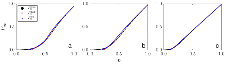
Figure SM1: Percolation diagrams for the Caenorhabditis Elegans duplex networks. Description of the various panels are identical to those of Fig. 1 of the main text. Order of appearance the duplexes is identical to the one of Table 1 of the main text.

Figure SM2: Percolation diagrams for the Drosophila Melanogaster duplex networks. Description of the various panels are identical to those of Fig. 1 of the main text. Order of appearance the duplexes is identical to the one of Table 1 of the main text.

Figure SM3: Percolation diagrams for the Homo Sapiens duplex networks. Description of the various panels are identical to those of Fig. 1 of the main text. Order of appearance the duplexes is identical to the one of Table 1 of the main text.

Figure SM4: Percolation diagrams for the NetSci Co-authorship duplex networks. Description of the various panels are identical to those of Fig. 1 of the main text. Order of appearance the duplexes is identical to the one of Table 1 of the main text.