Statistical Analyses for NANOGrav 5-year Timing Residuals

Abstract

In pulsar timing, timing residuals are the differences between the observed times of arrival and the predictions from the timing model. A comprehensive timing model will produce featureless residuals, which are presumably composed of dominating noise and weak physical effects excluded from the timing model (e.g. gravitational waves). In order to apply the optimal statistical methods for detecting the weak gravitational wave signals, we need to know the statistical properties of the noise components in the residuals. In this paper we utilize a variety of non-parametric statistical tests to analyze the whiteness and Gaussianity of the North American Nanohertz Observatory for Gravitational Waves (NANOGrav) 5-year timing data which are obtained from the Arecibo Observatory and the Green Bank Telescope from 2005 to 2010 (Demorest et al. 2013). We find that most of the data are consistent with white noise; Many data deviate from Gaussianity at different levels, nevertheless, removing outliers in some pulsars will mitigate the deviations.

1 Introduction

Pulsar timing as a powerful technique has achieved many of the most important science results in the pulsar astronomy. Timing of single pulsars has been used as a probe of the dispersive interstellar medium (Cordes & Lazio 2002), to test the theories of gravitation in the strong field regime (Damour & Taylor 1992; Stairs 2003; Kramer et al. 2006), to discover the first extraplanet system (Wolszczan & Frail 1992), to constrain the nuclear equation of state of neutron star (Demorest et al. 2010; Lattimer & Prakash 2007, 2010). It has provided the first evidence of the existence of gravitational waves (Taylor & Weisberg 1982, 1989). Timing a number of pulsars and analyzing the data coherently can be used to search for the irregularity of terrestrial time standard and develop a time-scale based on pulsars (Hobbs et al. 2012), and to deepen our understanding of solar system dynamics (Champion et al. 2010). Amazingly it can be operated as a galactic scale detector for very-low frequency gravitational waves (Hellings & Downs 1983; Foster & Backer 1990; Jenet et al. 2005).

Pulsar timing array (PTA) is an experiment to regularly observe a set of millisecond pulsars (MSPs). Currently, three PTAs, i.e., the North American Nanohertz Observatory for Gravitational Waves (NANOGrav, Demorest et al. (2013)), the Parkes Pulsar Timing Array (PPTA, Manchester et al. (2013)) and the European Pulsar Timing Array (EPTA, Ferdman et al. (2010)), have started to produce astrophysically important results. These PTAs compose the International Pulsar Timing Array (IPTA, Manchester (2013); McLaughlin (2014)) with approximately 50 pulsars regularly monitored. The first data combination has been released (Verbiest et al. 2016).

The PTA is sensitive to the very low frequency ($10^{-9}$–$10^{-7}$ Hz) gravitational waves (GWs), which is complementary to the ground based interferometric detectors (e.g., LIGO (Abbott et al. 2009) and Virgo (Accadia et al. 2011)) running in the high frequency band ($10-10^{3}$ Hz), and the space based laser rangers (e.g., eLISA (Seoane et al. 2013) and TianQin (Luo et al. 2016)) proposed for the low frequency band (0.1 mHz–0.1 Hz). Potential sources of GWs in the very low frequencies include the supermassive black hole binaries (Jaffe & Backer 2003; Wyithe & Loeb 2003; Sesana et al. 2008), the cosmic strings (Damour & Vilenkin 2005; Ölmez et al. 2010), and the relic gravitational waves (Grishchuk 2005).

At the current timing precision, it is very likely that the noises of different kinds are the dominating components of the timing residuals (Jenet et al. 2006; van Haasteren et al. 2011; Demorest et al. 2013; Shannon et al. 2013; Arzoumanian et al. 2014). On the one hand, to improve timing precision at the longest timescale, it is very important to have a comprehensive understanding of the sources (e.g., radiometer, pulse phase jitter, diffractive interstellar scintillation) and the characteristics of the noise in TOAs, and identify mitigation methods to reduce the noise (Cordes & Shannon 2010; Wang 2015). On the other hand, many data analysis methods designed for detecting the weak GW signals (Corbin & Cornish 2010; Babak & Sesana 2012; Ellis et al. 2012; Wang et al. 2014, 2015; Zhu et al. 2015, 2016) are usually geared to work well for the data owning some specific statistical properties. Blindly applying these data analysis strategies and pipelines without checking the presumptions may lead to nonsensical results (Tiburzi et al. 2016). In this paper, as a first step of noise characterization, we implement a suite of robust non-parametric statistical tools to test the most important noise properties, namely the whiteness and the Gaussianity, of the NANOGrav 5-year (2005–2010) data published in Demorest et al. (2013).

Using these tools, we found that most of the frequency separated data are individually consistent with the whiteness assumption, except the high frequency data from PSR J2145–0754 and J2317+1439 which show mild deviations. However, combining the data from different frequencies as one set causes significant deviations for PSR J0613–-0200, J1455–3330, J1744–1134, J1909–3744, J1918–0642 and J2317+1439. We found that this may be due to the minute inaccuracy of DM estimation for these pulsars with the current observation strategy. For the Gaussianity, most of the data show different levels of deviation, however, removing outliers in some pulsars would reduce the deviations.

The rest of the paper is organized as follows. In Sec. 2, a brief description of the observation and the data set is given. We use the zero-crossing method to test the whiteness of the data in Sec. 3, and use the descriptive statistics and the hypothesis testings to check the Gaussianity in Sec. 4. Demonstrations of these analyses on 3 pulsars are presented in Sec. 5. The paper is concluded in Sec. 6.

2 Observations and data

The NANOGrav collaboration has conducted observations with the Arecibo Observatory (AO) and the Green Bank Telescope (GBT), the two largest single dish radio telescopes to date. Currently 37 MSPs (Arzoumanian et al. 2015) have been regularly timed by the NANOGrav. The first five years data (2005–2010) for 17 of the MSPs along with the upper limit on the GW stochastic background have been published in Demorest et al. (2013). In order to precisely analyze the time dependent dispersion measure (DM) and frequency dependent pulse shape, two receivers operating at 1.4 GHz and 430 MHz for AO and 1.4 GHz and 820 MHz for GBT have been used in most of the observations. Observations using two different receivers were not simultaneous. At AO, the observations from the two bands were obtained within 1 hour; whereas at GBT, the separation could be up to a week. All observations during this 5 years have been carried out by the identical pulsar backends, i.e. the Astronomical Signal Processor (ASP) at AO and the Green Bank Astronomical Signal Processor (GASP) at GBT, in which the input analog signal is split into 32 4 MHz channels (sub-bands). Due to the limitation of the real-time computation load or the receiver bandpass, typically 16 channels would be processed in most observations. The cadence between observation sessions is typically 4-6 weeks. There is a gap in the observations of all pulsars in 2007 due to the maintenance at both telescopes.

The data product from an observation epoch is the pulse time of arrival (TOA) which is the time of the radio emission from a fiducial rotation phase of the pulsar arriving at the telescope. The standard TOA estimation includes polarization calibration, pulse profile folding, profile template creation, and TOA measurement by correlating folded profile and profile template. Those steps are integrated in the package PSRCHIVE (Hotan et al. 2004) and ASPFitsReader (Ferdman 2008). Both packages are used for cross-checking of errors which otherwise would hardly be targeted.

The next step of timing analysis is to fit the observed TOAs of each pulsar to a timing model. The timing model contains a set of physical parameters which account for the pulsar’s rotation (spin period, spin period derivatives), astrometry (position, proper motion), interstellar medium (dispersion measure), binary orbital dynamics, etc. This procedure is executed in the standard timing analysis package TEMPO2 (Hobbs et al. 2006; Edwards et al. 2006) via a weighted least square fitting. The so-called post-fit timing residuals are the differences between the measured TOAs and the TOAs predicted by this model. A positive residual means that the observed pulse arrives later than expected. The timing residuals potentially contain the stochastic noise from various sources and the physical effects that are not included in the timing model. One can refer to Demorest et al. (2013) for a thorough account on the NANOGrav observation strategy and timing analysis.

We can generate multiple timing residuals, denoted as $r(t,\nu)$, from the timing analysis of the NANOGrav data set, where $t$ is the time of observation of a pulse in the Modified Julian Date (MJD), $\nu$ is the central frequency of a channel. To simplify the study of timing effects induced by achromatic physical processes (e.g. gravitational wave), we can average the timing residuals from the TOAs registering the same rotation phase of the pulsar. If there are only TOAs from one pulsar rotation in an observation epoch (true for most observations), this averaged residual will equal to the daily averaged residual used in Fig. 1 of Demorest et al. (2013) and in Perrodin et al. (2013). The averaged residual $r_{I}$ for the $I$-th observation epoch in the data of a pulsar is

$$r_{I}=\frac{\sum\nolimits_{i=1}^{N_{I}}r_{Ii}\sigma_{Ii}^{-2}}{\sum\nolimits_{i=1}^{N_{I}}\sigma_{Ii}^{-2}}\,,$$ (1)

where $r_{Ii}=r(t_{I},\nu_{i})$ is the post-fit multi-frequency timing residual from the $i$-th frequency channel at the $I$-th observation epoch, $N_{I}$ is the number of frequency channels, and $\sigma_{Ii}$ is the uncertainty for the corresponding TOA. The uncertainty associated with the averaged residual is

$$\sigma_{I}=\sqrt{\left(\sum\nolimits_{i=1}^{N_{I}}\sigma_{Ii}^{-2}\right)^{-1}\frac{1}{N_{I}-1}\sum\nolimits_{i=1}^{N_{I}}(r_{Ii}-r_{I})^{2}\sigma_{Ii}^{-2}}\,.$$ (2)

Eq. 2 is the standard deviation of Eq. 1 with correction of underestimation of errors in TOA. This estimator is suitable when $\sigma_{Ii}$ does not include all the noise sources associated with TOAs. In addition, since we have used two independent receivers not simultaneously, we will separate the low frequency and high frequency averaged residuals and test them independently in our analysis.

The averaged timing residuals can be used as inputs of the GW detection pipelines. One advantage of averaging is that it reduces the random noise components across different frequency channels while keeps the achromatic GW signals intact. Besides, the averaged residuals provide a quantitative way to compare with the data from the EPTA (Ferdman et al. 2010; Lentati et al. 2015) and the PPTA (Manchester et al. 2013), which have routinely produced a single TOA per observation epoch.

3 Whiteness test

In this section, we test the consistency of the averaged timing residuals with the white noise assumption for each pulsar. The white noise time series is statistically uncorrelated in time, while the distribution of its values does not necessarily adhere to any specific probability distribution (Gaussian, Poisson, etc.). If evenly sampled, we can use Fourier analysis to calculate the power spectrum of the time series and to check whether it is consistent with a flat spectrum in the interested frequency range. However the pulsar timing data are usually not evenly sampled, i.e. the observation cadence varies, so that this conventional spectral analysis is not applicable. The Lomb-Scargle periodgram (Lomb 1976; Scargle 1982) which is designed for unevenly sampled data suffers from occasional large gaps between observations (see Fig. 1 in Demorest et al. (2013)), as well as limited data volume for each pulsar (see Table 2 for detailed numbers).

It turns out that after subtracting the mean value the number of the zero-crossing $Z_{W}$ of a white noise time series is a Gaussian random variable,

$$Z_{W}\sim\mathcal{N}(\mu_{Z_{W}},\sigma_{Z_{W}}^{2})\,,$$ (3)

where the expected value $\mu_{Z_{W}}=(N-1)/2$ and the standard deviation $\sigma_{Z_{W}}=\sqrt{N-1}/2$. The zero-crossing test is to check how large the number of the zero-crossing for a time series is different from the expectation. It is designed in the time domain, thus applicable to unevenly sampled data with gaps. This test is not sensitive to any non-stationarity of the statistics of the white noise, such as the case where the white noise has a jump in variance at some epoch because of a change in instrumentation. It is implicit that the white noise is “dense” which means that all data values are non-zero and stochastic (Papoulis 1984). Other kinds of white noise, such as the shot noise with a low shot rate will not conform to the zero-crossing test described here.

In Table 1, we show the results of the zero-crossing test for the frequency separated averaged residuals as well as the total averaged residuals (by combining the high and low frequency averaged residuals and sorting them in the ascending order of corresponding TOAs) for 17 pulsars. $\text{N}_{\text{crs}}$, is the actual number of the zero-crossing for the data, $\Delta$ is the difference between $\mu_{Z_{W}}$ and $\text{N}_{\text{crs}}$. The significance of the test is measured by how large $\Delta$ is comparing with $\sigma_{Z_{W}}$. If $|\Delta|<2\sigma_{Z_{W}}$ ($>$5% in p-value ), the data is said consistent with white noise (labeled by ‘Y’); if $3\sigma_{Z_{W}}>|\Delta|>2\sigma_{Z_{W}}$, it is said mildly deviated from white noise (‘n’); and if $|\Delta|>3\sigma_{Z_{W}}$, it is said strongly deviated from white noise (‘N’). We defer the detailed discussion and possible interpretation of these results to Sec. 5 to consolidate with the results from the Gaussianity tests.

4 Gaussianity test

In this section, we first use the descriptive statistics, namely the histogram and the Q-Q plot, to visually inspect the general features of the data. Then we implement a suite of inferential statistical tests to quantitatively measure the deviations from the Gaussianity. The observation conditions during the 5 years had been changing due to a number of factors, for instance, radiometer noise, interstellar scintillation and instrument. Therefore the underlying noise random variables at different frequencies and epochs are heteroscedastic. These changes are reflected in the variations of the error bars (e.g., for the averaged residuals showed in Fig. 1, 4 and 7). This feature is treated here by a simple normalization, so that the tested time series are from the same underlying distribution. For the averaged residuals, it is to normalize each residual from Eq. 1 by its associated uncertainty calculated in Eq. 2; While for the multi-frequency residuals, it is to normalize each residual by the uncertainty associated with its TOA.

The inferential statistics based on the statistical hypothesis testing theory argues against a null hypothesis (Gaussianity) as in the mathematical proof by contradiction. First, the data are summarized into a single number called the test statistic, which follows a certain probability distribution. Second, the p-value are calculated based on this distribution assuming that the null hypothesis is true. The lower the p-value is, the smaller the chance that the sample comes from a Gaussian distribution is.

One often rejects the null hypothesis when the p-value is less than the pre-assigned significance level which is usually 0.05. However, the power of the tests decreases as the sample size decreasing. It is a common practice to declare the significance level at higher values, such as 0.1 or 0.2 for a small sample in order to detect possible deviation that may be essential. This is an important point since the data sets that we will test vary largely in size (cf. Table 2).

To avoid possible bias in different tests, the significance of the Gaussianity test is measured by the averaged p-value $p$ of five tests, among which the Shapiro-Wilk test (S-W) and the Shapiro-Francia test (S-F) are the order statistics; the Anderson-Darling test (A-D), the Cramér-von Mises test (C-vM) and the Lilliefors test (Lillie) are base on the empirical distribution function (EDF). The results are summarized in Table 2. For multi-frequency residuals, if $p>0.05$, the data is said consistent with the Gaussianity (labeled by ‘Y’); if $0.05>p>10^{-3}$, the data is said mildly deviated from the Gaussianity (‘n’); and if $p<10^{-3}$, the data is said strongly deviated from the Gaussnianity (‘N’). For averaged residuals, the criterion intervals are set to be $p>0.1$ (‘Y’), $0.1>p>2\times 10^{-3}$ (‘n’), and $p<2\times 10^{-3}$ (‘N’), respectively. The p-values of all tests are only showed for three pulsars in the legends of Fig. 3, 6, and 9.

5 Results

The results for the whiteness and Gaussianity tests are summarized in Table 1 and Table 2. Here, we demonstrate the tests for three pulsars in details.

5.1 PSR J0613-0200

The frequency separated averaged timing residuals of PSR J0613-0200 are shown in Fig. 1. The red asterisks with error bars represent the high-frequency (1.4 GHz) residuals, and blue short-bars with error bars represent the low frequency (820 MHz) residuals. Apparently the high frequency residuals have larger variance than the low frequency residuals, and the high frequency error bar for this pulsar is a factor of a few larger than the low frequency error bars. This is mainly due to the fact that the mean flux density at high frequency is lower than that of low frequency according to the power-law spectrum of the flux density. For similar integration time, this will result in a larger uncertainty in the measurement of TOA by correlating lower S/N folded pulse with template pulse profile (Taylor 1992).

From Table 1 we can see that the low frequency and high frequency residuals are individually consistent with the white noise assumption. However when they are combined into a single time series, the total residuals show more zero-crossing than expected, the deviation for this pulsar is more than $4\sigma$. We found that the excess of zero-crossing is caused by the error in the estimated values of time dependent DM with the observation strategy adopted in the NANOGrav 5-year data. However, we defer the detailed discussion to Sec. 6.

After normalizing the averaged residuals by their associated error bars, we notice that in Fig. 2 and 3 the standard deviation of the low frequency residuals is significantly smaller than unity which hints that the error bar calculated for the low frequency averaged data are overestimated. Therefore the combined residuals deviate from the Gaussian distribution, even if the low frequency averaged residuals and high frequency averaged residuals are both consistent with the Gaussian distribution individually. It may suggest that in order to properly combine the data from different frequency bands in GW detection algorithms, we may need to add a scaling parameter for each frequency band that is similar to the EFAC parameter used in timing analysis. The post-fit multi-frequency residuals are mildly deviated from the Gaussian distribution.

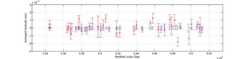
Figure 1: Frequency separated averaged timing residuals with error bars for J0613–0200. The red asterisks represent high frequency data, while the blue short-bars represent low frequency data.

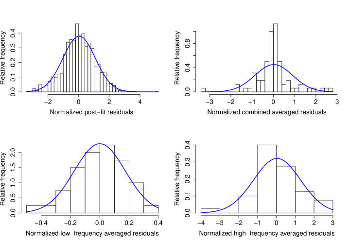
Figure 2: Histograms for the post-fit multi-frequency residuals (top-left), total (top-right), low-frequency (bottom-left), and high-frequency (bottom-right) averaged residuals of J0613–0200. The blue curve is the Gaussian distribution with the same mean and variance as the data.

Figure 3: Quantile-Quantile plots for the post-fit multi-frequency residuals (top-left), total (top-right), low-frequency (bottom-left), and high-frequency (bottom-right) averaged residuals of J0613–0200. The p-values of individual test are listed in the legends.

5.2 PSR J1012+5307

From Table 1, we can see that the low-frequency, high-frequency, and total averaged residuals are all consistent with the white noise assumption. From Table. 2, we can see that the high frequency averaged and post-fit multi-frequency residuals are mildly deviated from the Gaussian distribution, while the low frequency averaged and total averaged residuals are strongly deviated from the Gaussian distribution.

We notice from Fig. 6 that for the post-fit residuals the results from the order statistics tests (strong deviation) are not consistent with the EDF tests (mild deviation). This is ascribed to that the order statistic tests are sensitive to the outliers which can be identified from Fig. 5 and 6. After removing two outliers in the residuals, the results from the order statistics are improved rapidly (S-W = $8.3\times 10^{-4}$, S-F = $4.5\times 10^{-4}$), and become more consistent with the other tests.

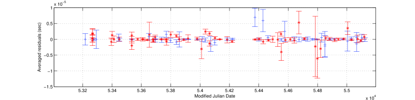
Figure 4: Frequency separated averaged timing residuals with error bars for J1012+5307. The red asterisks represent high frequency data, while the blue short-bars represent low frequency data.

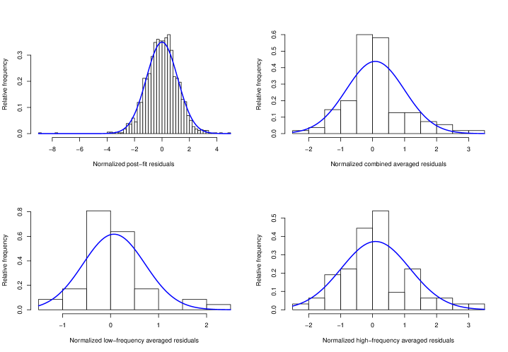
Figure 5: Histograms for the post-fit residuals, total, low-frequency, and high-frequency averaged residuals of J1012+5307. The blue curve is the Gaussian distribution with the same mean and variance as the data.

Figure 6: Quantile-Quantile plots for the post-fit residuals, total, low-frequency, and high-frequency averaged residuals of J1012+5307. The p-values of individual test are listed in the legends.

5.3 PSR J1713+0747

PSR J1713+0747 is the only one among the 17 pulsars that has been observed by both the AO and the GBT. Currently, it is the best timed pulsar in the NANOGrav. It has been observed extensively in three frequency bands, i.e. 820 MHz, 1.4 GHz, and 2.3 GHz, which are marked by blue short-bars, red asterisks, and black squares respectively in Fig. 7. (There are actually two sessions conducted in 2.7 GHz at the AO which are not included in this analysis.)

The three frequency separated averaged residuals are all consistent with the white noise assumption individually, whereas the total averaged residuals are mildly deviated from it. Except the residuals from 2.3 GHz band, the residuals from the other two bands are all strongly deviated from the Gaussian distribution. And removing a few outliers improves the statistics considerably.

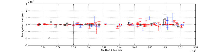
Figure 7: Frequency separated averaged timing residuals with error bars for J1713+0747. The blue short-bars represent 820 MHz data, the red asterisks represent 1.4 GHz data, and black squares represent 2.3 GHz data.

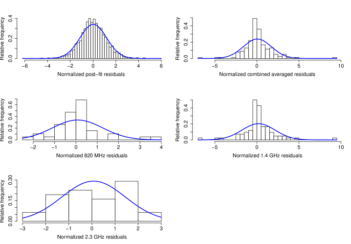
Figure 8: Histograms for the post-fit residuals, total, 820 MHz, 1.4 GHz, and 2.3 GHz averaged residuals of J1713+0747. The blue curve is the Gaussian distribution with the same mean and variance as the data.

Figure 9: Quantile-Quantile plots for the post-fit residuals, total, 820 MHz, 1.4 GHz, and 2.3 GHz averaged residuals of J1713+0747. The p-values of individual test are listed in the legends.

6 Summary and discussions

In this paper we utilized a set of non-parametric statistical tests to analyze the NANOGrav 5-year timing residuals for 17 pulsars. The zero-crossing has been used to test the whiteness assumption for the averaged timing residuals. The results are summerized in Table 1. Both descriptive and inferential statistical methods have been used to test the Gaussianity for the post-fit multi-frequency and averaged timing residuals. The results are summarized in Table 2. The histogram and Q-Q plots for 3 pulsars are shown for demonstration purpose.

We found that for most cases, except the high frequency averaged residuals of J2145-0750 and J2317+1439, the frequency separated averaged residuals are consistent with the white noise assumption. However, when they are combined, the total averaged residuals of 5 pulsars show strong deviations from whiteness (‘N’) and 4 pulsars show mild deviations from whiteness (‘n’).

In principle, the total averaged residuals can be modeled by combining two time series $x_{1}(t_{i})$ and $x_{2}(t^{\prime}_{j})$ representing the low frequency and high frequency averaged residuals, where $t_{i}$ ($i=1,2,3,...,N_{1}$) and $t^{\prime}_{j}$ ($j=1,2,3,...,N_{2}$) are not necessarily identical or evenly spaced. If the two time series are separately drawn from white noise processes, then the number of zero-crossing of the combined time series (sorted in the ascending order of the union of $\{t_{i}\}$ and $\{t^{\prime}_{j}\}$) is a Gaussian random variable with the expectation equals to $(N1+N2-1)/2$ and the variance equals to $(N1+N2-1)/4$.

The cumulative zero-crossings of total averaged residuals with low and high frequency averaged residuals for PSR J1012+5307 and J0613–0200 are shown in Fig. 10 and Fig. 11. Asterisks represent the number of zero-crossing (y-axis) added up to this time (x-axis), it is equivalent to the zero-crossings for the data within an enlarging time window with the left end fixed at the beginning of the time series and the right end sliding to the time of this data point. The solid curves are the expected numbers of zero-crossing of the data size within the window and the dash-dot lines are the $1\sigma$ contours. They are all monotonic functions of time. Red, black, and blue represent the low frequency, high-frequency, and total averaged residuals.

For J1012+5307, the cumulative zero-crossings of low frequency, high frequency and total averaged residuals follow closely to the expected values within $1\sigma$ contour. This is exactly what is expected for a combination of two white noise time series. In contrast, for J0613–0200, although the low frequency and high frequency zero-crossings follow closely to the expectations as in J1012+5307, the combined data shows strong deviation from its expectation. In Fig. 11, it starts to deviate away from the beginning of the time series, and the final deviation is more than $4\sigma$. As stated, this strong deviation for the combined averaged residuals also appears in other pulsars in Table 1.

In fact, the apparent excess of zero-crossing is mainly due to the strategy of fitting the physical parameters especially the time-variable DM in timing analysis. It is the practice in the NANOGrav 5-year data timing analysis to include a piecewise-constant DM(t) function in the fitting model along with the other parameters (rotation, astrometry, binary dynamics, and pulse profile evolution). The window for a constant DM value is typically 15 days which include a couple of observations conducted at high and low frequencies. However, any fluctuation of DM within this window or inaccuracy of the DM fit will introduce additional error between the adjacent averaged timing residuals from two widely separated bands as follows,

$$\delta t\simeq 4.15\times 10^{6}~{}\text{ms}\times\delta\text{DM}\times\left(f_{1}^{-2}-f_{2}^{-2}\right)\,.$$ (4)

Here, $f$ is measured in MHz. For J0613–0200, the uncertainty of DM measurement ($\sim 10^{-4}\rm{cm^{-3}pc}$) can produce several hundreds of nanosecond of fluctuation between low (820 MHz) and high frequency (1.4 GHz). This is comparable with the RMS of averaged timing residual reported in Table 2 of Demorest et al. (2013). The minute error of DM will cause low frequency TOAs tend to be advanced and high frequency TOAs delayed or vise versa (the DM fit will tend to move the two sets of TOAs from low and high frequencies, so that their averaged residual is zero) which will produce extra zero-crossings between low and high frequency timing residuals within a DM fitting window. This effect is expected to be seen more clearly in the GBT observed pulsars, since the time separation between two observation bands is much larger and the frequency coverage (crucial for the DM measurement) is significantly smaller than the AO. We found that all 5 pulsars that have total averaged residuals strongly deviated from whiteness, whereas frequency separated averaged residuals are all consistent, are observed by the GBT.

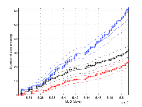
Figure 10: Cumulative zero crossing of PSR J1012+5307, y-axis is the number of zero-crossing, x-axis is the modified Julian date at which the observations are made. See text for details.

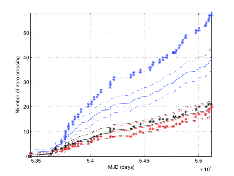
Figure 11: Cumulative zero crossing of PSR J0613–0200, y-axis is the number of zero-crossing, x-axis is the modified Julian date at which the observations are made. See text for details.

The Gaussianity is one of the fundamental assumptions used in most if not all of the GW detection methods. The tests here suggest that many of the NANOGrav pulsars show deviations from the Gaussian distribution at different levels. The deviations in some data, averaged and multi-frequency post-fit residuals, can be mitigated by removing a few outliers. This strategy is consistent with the so called robust statistics (Allen et al. 2002, 2003) which is used to confront the non-Gaussianity in GW data analysis by clipping samples with values locating in the outlier part of the probability distribution. It is robust in the sense that it is close to optimal for the Gaussian noise but far less sensitive to the large excess events than the conventional statistics. Moreover, for the purpose of detection, coherent methods (e.g., Wang et al. (2014, 2015)) have been shown to be robust against non-Gaussianity for detecting deterministic GW signals (Finn 2001). Alternative method in wavelet domain has also been explored for searching stochastic GW signals in non-Gaussian and non-stationary noise (Klimenko et al. 2002) with ground based GW detectors. The results here suggest that these methods should be investigated for the GW detection with PTA in the future.

Table 1: Results for the zero-crossing test. Consistent with whiteness – ‘Y’, mildly deviated – ‘n’, and strongly deviated – ‘N’.

Source	Low-frequency band					High-frequency band					Combined
	$\text{N}_{\text{crs}}$	$\mu_{Z_{W}}$	$\Delta$	$\sigma_{Z_{W}}$	Y/n/N	$\text{N}_{\text{crs}}$	$\mu_{Z_{W}}$	$\Delta$	$\sigma_{Z_{W}}$	Y/n/N	$\text{N}_{\text{crs}}$	$\mu_{Z_{W}}$	$\Delta$	$\sigma_{Z_{W}}$	Y/n/N
J0030+0451	12	11.5	-0.5	2.4	Y	14	12.5	-1.5	2.5	Y	27	24.5	-2.5	3.5	Y
J0613–0200	20	19.5	-0.5	3.1	Y	19	19.5	0.5	3.1	Y	58	39.5	-18.5	4.4	N
J1012+5307	26	23	-3	3.4	Y	34	31	-3	3.9	Y	62	54.5	-7.5	5.2	Y
J1455–3330	22	20	-2	3.2	Y	23	22	-1	3.3	Y	58	42.5	-15.5	4.6	N
J1600–3053	13	10.5	-2.5	2.3	Y	13	12.5	-0.5	2.5	Y	33	23.5	-9.5	3.4	n
J1640+2224	18	16.5	-1.5	2.9	Y	14	15.5	1.5	2.8	Y	35	32.5	-2.5	4.0	Y
J1643–1224	26	23	-3	3.4	Y	22	24.5	2.5	3.5	Y	62	48	-14	4.9	n
J1713+0747	19	18.5	-0.5	3	Y	46	41.5	-4.5	4.6	Y	-	-	-	-	-
J1713+0747	-	-	-	-	-	18	15	-3	2.7	Y	94	76	-18	6.2	n
J1744–1134	25	23.5	-1.5	3.4	Y	33	29.5	-3.5	3.8	Y	70	53.5	-16.5	5.2	N
J1853+1308	21	20	-1	3.2	Y	-	-	-	-	-	19	21	2	3.2	Y
B1855+09	17	18	1	3.0	Y	17	15.5	-1.5	2.8	Y	46	34	-12	4.1	n
J1909–3744	17	17	0	2.9	Y	17	16	-1	2.8	Y	52	33.5	-18.5	4.1	N
J1910+1256	13	15	2	2.7	Y	3	2.5	-0.5	1.1	Y	21	18	-3	3	Y
J1918–0642	20	19.5	-0.5	3.1	Y	29	26.5	-2.5	3.6	Y	64	46.5	-17.5	4.8	N
B1953+29	14	11	-3	2.3	Y	-	-	-	-	-	16	12	-4	2.4	Y
J2145–0750	15	10.5	-4.5	2.3	Y	18	11.5	-6.5	2.4	n	31	22.5	-8.5	3.4	n
J2317+1439	26	21	-5	3.2	Y	27	20	-7	3.2	n	56	41.5	-14.5	4.6	N

Table 2: Results for the inferential statistical tests of the Gaussianity. The numbers represent the sample size. For post-fit residuals, if $p>0.05$, the data is consistent with Gaussianity (labeled by ‘Y’), if $0.05>p>10^{-3}$, the data is mildly deviated from Gaussianity (‘n’), and if $p<10^{-3}$, the data is strongly deviated from Gaussnianity (‘N’). For averaged residual, the criterion intervals are set to be $p>0.1$ (‘Y’), $0.1>p>2\times 10^{-3}$ (‘n’), and $p<2\times 10^{-3}$ (‘N’) respectively. ‘NA’ appears when the test is not applicable to such small sample size.

Source	$P$	DM	Averaged timing residuals						Post-fit
	(ms)	(pc cm-3)	327 MHz	430 MHz	820 MHz	1.4 GHz	2.3 GHz	Comb.
J0030+0451	4.87	4.33	-	24 N	-	26 n	-	50 N	545 Y
J0613–0200	3.06	38.78	-	-	40 Y	40 Y	-	80 N	1113 n
J1012+5307	5.26	9.02	-	-	47 N	63 n	-	110 N	1678 n
J1455–3330	7.99	13.57	-	-	41 n	45 Y	-	86 N	1100 n
J1600–3053	3.60	52.33	-	-	22 n	26 n	-	48 n	625 Y
J1640+2224	3.16	18.43	-	34 N	-	32 N	-	68 N	631 N
J1643–1224	4.62	62.42	-	-	47 N	50 Y	-	97 N	1266 N
J1713+0747	4.57	15.99	-	-	38 N	84 N	31 Y	153 N	2368 N
J1744–1134	4.07	3.14	-	-	48 N	60 Y	-	108 N	1617 N
J1853+1308	4.09	30.57	-	-	-	41 Y	2 NA	43 Y	497 Y
B1855+09	5.36	13.30	-	37 N	-	32 Y	-	69 n	702 N
J1909–3744	2.95	10.39	-	-	35 n	33 Y	-	68 N	1001 N
J1910+1256	4.98	34.48	-	-	-	31 Y	6 Y	37 Y	525 Y
J1918–0642	7.65	26.60	-	-	40 Y	54 n	-	94 N	1306 Y
B1953+29	6.13	104.50	-	-	-	23 Y	2 NA	25 Y	208 Y
J2145–0750	16.05	9.03	-	-	22 N	24 Y	-	46 n	675 n
J2317+1439	3.45	21.90	43 n	41 n	-	-	-	84 N	458 n