Abstract

The goal of causal inference is to understand the outcome of alternative courses of action. However, all causal inference requires assumptions. Such assumptions can be more influential than in typical tasks for probabilistic modeling, and testing those assumptions is important to assess the validity of causal inference. We develop model criticism for Bayesian causal inference, building on the idea of posterior predictive checks to assess model fit. Our approach involves decomposing the problem, separately criticizing the model of treatment assignments and the model of outcomes. Conditioned on the assumption of unconfoundedness—that the treatments are assigned independently of the potential outcomes—we show how to check any additional modeling assumption. Our approach provides a foundation for diagnosing model-based causal inferences.

1 Introduction

Consider the problem of understanding the “treatment effect” of an intervention, such as giving a drug to patients with a specific disease. In the language of Neyman, (1923); Rubin, (1974), each individual has a potential outcome when given the drug and a potential outcome when not given the drug. One measurement of the causal effect is the average difference (over individuals) between those potential outcomes. In the language of graphical models, this is framed as evaluating the impact of an intervention on random variables in a probabilistic graph (Pearl,, 2000). The fundamental problem of causal inference is that we do not observe both potential outcomes for any individual at the same time (Holland,, 1986); to estimate the causal effect, we need assumptions about the data generating process.

Assumptions are important to all probabilistic modeling, but especially for making causal inferences. In such inferences, we make strong assumptions about how treatments are assigned to individuals and each individual’s distribution of potential outcomes. Given assumptions about the data, there are myriad methods for model-based causal inference (Pearl,, 2000; Robins et al.,, 2000; Morgan and Winship,, 2014; Imbens and Rubin,, 2015).

We focus on Bayesian methods. Bayesian methods have a long history in causal inference (Rubin,, 1974; Raudenbush and Bryk,, 1986). In recent years, applied researchers are increasingly able to fit complicated probabilistic models to capture fine-grained phenomena—for example, high-dimensional regressions with regularization to handle large numbers of predictors (Maathuis et al.,, 2009; Belloni et al.,, 2014), or hierarchical models to adjust for unmeasured covariates and capture heterogeneity in treatment effects (Hirano et al.,, 2000; Feller and Gelman,, 2014).

However, for applied researchers, Bayesian methods can been difficult to use. One reason for this is the lack of diagnostic tools to check such complicated models. For high-dimensional and massive data, prior information—beliefs that capture our assumptions on the data generating process—can be essential in order to draw efficient causal inferences (Bottou et al.,, 2013; Peters et al.,, 2015; Johansson et al.,, 2016). This in turn necessitates ways to check the modeling assumptions.

We develop model criticism for Bayesian causal inference. We build on the idea of posterior predictive checks (ppcs) (Box,, 1980; Rubin,, 1984; Gelman et al.,, 1996) to adapt goodness-of-fit style calculations to causal modeling. We decompose the problem, separately criticizing the two components that make up a causal model: the model of treatment assignments and the model of outcomes.

We emphasize that there are several causal assumptions that our method cannot check. First, we do not check unconfoundedness. There are many existing methods for this, such as robustness tests (Angrist,, 2004; Lu and White,, 2014; Chen and Pearl,, 2015) and estimation of pseudo causal effects (Rosenbaum et al.,, 1987; Heckman and Hotz,, 1989). The results of these methods do not directly test unconfoundedness—such tests are theoretically not possible (Pearl,, 2000)—but can lend plausibility to the assumption. Second, we do not check correlation between potential outcomes. This is also untestable as no pair of potential outcomes is observed for a single data point. In practice, we recommend using existing methods to understand the plausibility of these untestable assumptions, and then to apply our methods to check the additional assumptions.

In Section 2, we describe model-based causal inference with potential outcomes. In Section 3, we develop methods for checking the models and confirm their properties on simulated data. In Section 4, we show how the methods can be applied for real-world problems: an observational study on the effect of pest management in urban apartments and an educational experiment on the effect of television exposure on children.

1.1 Related Work

There has been little work on Bayesian model criticism for causal inference. Model checking is a frequent activity in the practice of propensity score analysis, typically for matching (Dehejia,, 2005; Austin,, 2009). Standard econometric texts (Greene,, 2003; Wooldridge,, 2010) discuss regression diagnostics and specification error. Neither of them considers a Bayesian treatment of diagnostics or how to check Bayesian methods for causal inference.

Our method borrows from the rich literature on doubly robust estimation (Robins and Rotnitzky,, 2001; Van der Laan and Robins,, 2003; Bang and Robins,, 2005) and inverse probability of treatment weighting (Rosenbaum and Rubin,, 1983; Heckman et al.,, 1998; Dehejia and Wahba,, 2002). Such methods are designed to mitigate selection bias, which arises from phenomena such as uncontrolled nonresponse and attrition, for the estimation of causal effects. In Section 3.3, we consider how such techniques can be applied for diagnosing model misfit.

Central to ppcs is the idea of predictive assessment: a model is evaluated by its predictions on future data given past information (Dawid,, 1984). This has come up in the context of causal inference via targeted learning and the super learner (Van der Laan and Rubin,, 2006; Van der Laan et al.,, 2007). In fact, targeted learning can be thought of as maximizing the statistical power for a given ppc (which we describe in Section 3).

In the context of missing data analysis, imputation of missing data has been a de facto standard for model checking (see, e.g., Chaloner, (1991); Gelman et al., (2005); Su et al., (2011)). This approach can also be applied for checking causal models. In Section 4, we discuss it in detail and compare it to our approach.

2 Causal models

We describe causal models in terms of the potential outcomes framework (Neyman,, 1923; Rubin,, 1974; Imbens and Rubin,, 2015). Let $\boldsymbol{\mathbf{y}}(0),\boldsymbol{\mathbf{y}}(1)$ be the set of potential outcomes under a binary treatment $\boldsymbol{\mathbf{a}}\in\{0,1\}$; and let $y_{i}(a)$ be the outcome when an individual $i$ is exposed to treatment $a$. We use uppercase, e.g., $\boldsymbol{\mathbf{Y}}(0),\boldsymbol{\mathbf{Y}}(1)$, to denote random variables and lowercase, e.g., $\boldsymbol{\mathbf{y}}(0),\boldsymbol{\mathbf{y}}(1)$, to denote their realizations. (See Appendix for a table of our notation.)

2.1 Definition of a causal model

Let $x_{i}$ denote a set of covariates for an individual $i$. The potential outcomes arise from an outcome model,

$$\theta \sim p(\theta)$$

$$x_{i} \sim p(x)$$ (1)

$$(y_{i}(0),y_{i}(1)) \sim p(y(0),y(1)\,|\,\theta,x_{i}).$$

The potential outcomes are exchangeable across individuals; they are conditionally independent given the outcome parameters $\theta$ and covariates $x_{i}$.

Unfortunately we do not observe both potential outcomes for any individual. The outcome we observe is determined by the assignment model of the treatment indicators $a_{i}$. The treatment indicator $a_{i}$ equals one if we observe $y_{i}(1)$ and equals zero if we observe $y_{i}(0)$.

We consider the unconfounded assignment model. Each assignment is drawn conditional on the covariates $x_{i}$ and unknown assignment parameters $\phi$,

$$\begin{split}\phi&\sim p(\phi)\\ a_{i}&\sim p(a\,|\,x_{i},\phi).\end{split}$$ (2)

This model assumes unconfoundedness: $(Y(0),Y(1))\mathchoice{\mathrel{\hbox to0.0pt{$\displaystyle\perp$\hss}\mkern 2.0mu{\displaystyle\perp}}}{\mathrel{\hbox to0.0pt{$\textstyle\perp$\hss}\mkern 2.0mu{\textstyle\perp}}}{\mathrel{\hbox to0.0pt{$\scriptstyle\perp$\hss}\mkern 2.0mu{\scriptstyle\perp}}}{\mathrel{\hbox to0.0pt{$\scriptscriptstyle\perp$\hss}\mkern 2.0mu{\scriptscriptstyle\perp}}}A\,|\,X$. In other words, conditional on the covariates, the potential outcomes are independent of the treatment assignment. In missing data analysis, the assumption is known as strong ignorability (Little and Rubin,, 1987).

We combine the outcome and assignment model in a causal model. With an unconfounded assignment model, the causal model is

$$p(\theta,\phi,\boldsymbol{\mathbf{x}},\boldsymbol{\mathbf{y}}(0),\boldsymbol{\mathbf{y}}(1),\boldsymbol{\mathbf{a}})=$$ (3)

$$\hskip 20.00003ptp(\theta)p(\phi)p(\boldsymbol{\mathbf{x}})p(\boldsymbol{\mathbf{y}}(0),\boldsymbol{\mathbf{y}}(1)\,|\,\theta,\boldsymbol{\mathbf{x}})p(\boldsymbol{\mathbf{a}}\,|\,\phi,\boldsymbol{\mathbf{x}}).$$

We observe $\boldsymbol{\mathbf{x}}$, $\boldsymbol{\mathbf{a}}$, and $\boldsymbol{\mathbf{y}}(\boldsymbol{\mathbf{a}})$; all the other variables are latent.

For exposition, we make a few simplifications. Specifically, we assume: (1) the outcomes of an individual are independent of the assignment of other individuals; (2) the outcome and assignment model parameters are independent; and (3) the treatment assignment has binary support. The approach we describe extends beyond these settings.

2.2 Bayesian inference in a causal model

Given observed data $\{\boldsymbol{\mathbf{x}},\boldsymbol{\mathbf{a}},\boldsymbol{\mathbf{y}}(\boldsymbol{\mathbf{a}})\}$, we would like to calculate the posterior distribution of the assignment parameters $\phi$ and outcome parameters $\theta$. Let $\bar{\boldsymbol{\mathbf{a}}}$ denote the unobserved counterfactual assignments, i.e., $\bar{\boldsymbol{\mathbf{a}}}=1-\boldsymbol{\mathbf{a}}$. We marginalize out the counterfactuals to calculate the posterior,

$$\begin{split}p(\theta,\phi\,|\,\boldsymbol{\mathbf{y}}(\boldsymbol{\mathbf{a}}),\boldsymbol{\mathbf{a}},\boldsymbol{\mathbf{x}})&\propto p(\theta)p(\phi)p(\boldsymbol{\mathbf{a}}\,|\,\phi,\boldsymbol{\mathbf{x}})\\ &\times\int p(\boldsymbol{\mathbf{y}}(\boldsymbol{\mathbf{a}}),\boldsymbol{\mathbf{y}}(\bar{\boldsymbol{\mathbf{a}}})\,|\,\theta,\boldsymbol{\mathbf{x}})\operatorname{d}\!{\boldsymbol{\mathbf{y}}(\bar{\boldsymbol{\mathbf{a}}})}.\end{split}$$ (4)

Because of unconfoundedness, the posterior factorizes,

$$p(\theta\,|\,\boldsymbol{\mathbf{y}}(\boldsymbol{\mathbf{a}}),\boldsymbol{\mathbf{a}},\boldsymbol{\mathbf{x}})\propto p(\theta)\int p(\boldsymbol{\mathbf{y}}(\boldsymbol{\mathbf{a}}),\boldsymbol{\mathbf{y}}(\bar{\boldsymbol{\mathbf{a}}})\,|\,\theta,\boldsymbol{\mathbf{x}})\operatorname{d}\!{\boldsymbol{\mathbf{y}}(\bar{\boldsymbol{\mathbf{a}}})},$$

$$p(\phi\,|\,\boldsymbol{\mathbf{y}}(\boldsymbol{\mathbf{a}}),\boldsymbol{\mathbf{a}},\boldsymbol{\mathbf{x}})\propto p(\phi)p(\boldsymbol{\mathbf{a}}\,|\,\phi,\boldsymbol{\mathbf{x}}).$$

In other words, the assignment mechanism plays no role when inferring potential outcomes. Similarly, the potential outcomes play no role when inferring the assignment mechanism. Motivated by this consequence of ignorability (Rubin,, 1976; Dawid and Dickey,, 1977), we devise a method that separately checks the fitted parameters $\theta$ and $\phi$.

3 Model criticism for causal inference

Model criticism measures the degree to which a model falsely describes the data (Gelman and Shalizi,, 2012). We can never validate whether a model is true—no model will be true in practice—but we can try to uncover where the model goes wrong. Model criticism helps justify the model as an approximation or point to good directions for revising the model.

The central tool of model criticism is the posterior predictive check (ppc). It quantifies the degree to which data generated from the model deviate from the observed data (Box,, 1980; Rubin,, 1984; Gelman et al.,, 1996).

The procedure is:

1. Design a discrepancy function, a statistic of the data and hidden variables. A “targeted” discrepancy summarizes a specific component of the data, such as a quantile. An “omnibus” discrepancy is an overall summary of the data, such as the $\chi^{2}$ goodness of fit.

2. Form the realized discrepancy. It is the discrepancy evaluated at the observed data along with posterior samples of the hidden variables.

3. Form the reference distribution. It the distribution of the discrepancy applied to data sets from the posterior predictive distribution. In contrast to the realized discrepancy where the observations are fixed, the reference distribution is evaluated on samples of both observations and hidden variables.

4. Finally, locate the realized discrepancy in the reference distribution, e.g., by making a plot or by calculating a tail probability. If the realized discrepancy is unlikely, then the model poorly describes this function of the data and we revise the model. If it is reasonable, then this provides evidence that the model is justified.

ppcs are typically applied to validating non-causal models, especially for exploratory and unsupervised tasks (Yano et al.,, 2001; Royle and Dorazio,, 2008; Mimno and Blei,, 2011; Mimno et al.,, 2015). Here we extend this methodology to validating causal models.

3.1 Posterior predictive checks for causal models

We first consider the discrepancy function. Define a causal discrepancy to be a scalar function of the form,

$$T((\boldsymbol{\mathbf{y}}(0),\boldsymbol{\mathbf{y}}(1)),\boldsymbol{\mathbf{a}},\theta,\phi).$$ (5)

It is a function of all variables in the causal model of Eq.2.1: the potential outcomes $\boldsymbol{\mathbf{y}}(0),\boldsymbol{\mathbf{y}}(1)$, the treatment assignment $\boldsymbol{\mathbf{a}}$, the outcome model parameters $\theta$, and the assignment model parameters $\phi$. Depending on the check, it is a function of a subset of these variables.

In the original formulation of a ppc, the discrepancy was a function solely of observed data (Rubin,, 1984). Later work extended the discrepancy to also depend on latent parameters (Meng,, 1994; Gelman et al.,, 1996). The causal discrepancy of Eq.5 depends on observed outcomes and assignments, latent parameters, and unobserved outcomes, i.e., the counterfactual outcomes. Discrepancies of this form were studied in the context of missing data by Gelman et al., (2005).

We will use causal discrepancies to check each piece of the causal model. To complete the definition of a causal check, we must define the reference distribution and the realized discrepancy. In a ppc the reference distribution is the posterior predictive. This is the distribution that the data would have come from if the model were true.

Let $\boldsymbol{\mathbf{y}}(0)^{\rm rep},\boldsymbol{\mathbf{y}}(1)^{\rm rep},\boldsymbol{\mathbf{a}}^{\rm rep}$ denote replicated data from the posterior predictive distribution. Define the observed dataset $\mathcal{D}^{\rm obs}=\{\boldsymbol{\mathbf{x}},\boldsymbol{\mathbf{y}}(\boldsymbol{\mathbf{a}}),\boldsymbol{\mathbf{a}}\}$. We replicate the assignments and outcomes conditioned on $\mathcal{D}^{\rm obs}$,

$$\begin{split}\phi^{\rm rep}&\sim p(\phi\,|\,\mathcal{D}^{\rm obs})\\ \boldsymbol{\mathbf{a}}^{\rm rep}&\sim p(\boldsymbol{\mathbf{a}}\,|\,\boldsymbol{\mathbf{x}},\phi^{\rm rep})\\ \theta^{\rm rep}&\sim p(\theta\,|\,\mathcal{D}^{\rm obs})\\ \boldsymbol{\mathbf{y}}(0)^{\rm rep},\boldsymbol{\mathbf{y}}(1)^{\rm rep}&\sim p(\boldsymbol{\mathbf{y}}(0),\boldsymbol{\mathbf{y}}(1)\,|\,\boldsymbol{\mathbf{x}},\theta^{\rm rep}).\end{split}$$ (6)

This defines the reference distribution of the causal discrepancy of Eq.5.

A causal check compares the reference discrepancy to the realized discrepancy. The realized discrepancy is evaluated on observed data. When $T(\cdot)$ depends on latent variables—either assignment parameters, outcome parameters, or alternative outcomes—we replicate them from the reference distribution. (In that case the realization of the discrepancy is itself a distribution.) Following Gelman et al., (1996, 2005), the observed data are always held fixed at their observed values; only latent variables are replicated. This is in contrast to the reference distribution, which samples all of the variables. We note that in causal inference, we cannot use this strategy with the counterfactual outcomes; we will discuss this nuance below in Section 3.3.

We described the causal discrepancy, its reference distribution, and its realization. We now show how to use these ingredients to criticize causal models. We separate criticism into two components: criticizing the assignment model and criticizing the outcome model.

3.2 Criticizing the assignment model

The gold standard for validating causal models is a held-out experiment, where we have access to the assignment mechanism when validating against held-out outcomes (Rubin,, 2008). In observational studies, however, the assignment mechanism is unknown; we must model it with the goal of capturing the true distribution of the assignments. To check this aspect of the model, we apply a standard ppc. Under the assumption of unconfoundedness, we can check the assignment model with discrepancies $T(\boldsymbol{\mathbf{a}},\phi)$ that are functions of the assignment parameters $\phi$ and assignments $\boldsymbol{\mathbf{a}}$.

Algorithm 1 describes the procedure. It isolates the components of the model and data relevant to the assignment mechanism. First we calculate the realized discrepancy $T(\boldsymbol{\mathbf{a}},\phi^{\textrm{{rep}}})$; then we compare against the reference distribution $T(\boldsymbol{\mathbf{a}}^{\textrm{rep}},\phi^{\textrm{rep}})$. The reference distribution is simply the posterior predictive (Eq.6).

Input: Assignment model $p(\phi\,|\,\mathcal{D}^{\rm obs})p(\boldsymbol{\mathbf{a}}^{\rm rep}\,|\,\boldsymbol{\mathbf{x}},\phi)$, Discrepancy $T(\boldsymbol{\mathbf{a}},\phi)$.

Output: Reference distribution $p(T)$ and

            Realized discrepancy $T^{\rm obs}$.

for $s=1,\ldots,S$ replications do

       Draw assignment parameters $\phi^{s}\sim p(\phi\,|\,\mathcal{D}^{\rm obs})$.

       Draw assignments $\boldsymbol{\mathbf{a}}^{{\rm rep},s}\sim p(\boldsymbol{\mathbf{a}}^{\rm rep}\,|\,\boldsymbol{\mathbf{x}},\phi^{s})$.

       Calculate discrepancy $T^{{\rm rep},s}=T(\boldsymbol{\mathbf{a}}^{{\rm rep},s},\phi^{s})$.

       Calculate discrepancy $T^{{\rm obs},s}=T(\boldsymbol{\mathbf{a}},\phi^{s}).$

end for

Form reference distribution $p(T)$ from replications $\{T^{{\rm rep},s}\}$.

Form realized discrepancy $T^{\rm obs}$ from replications $\{T^{{\rm obs},s}\}$.

Algorithm 1 Criticism of the assignment model

Example.  Consider the average (marginal) log-likelihood of assignment,

$$\begin{split}T(\boldsymbol{\mathbf{a}})&=\frac{1}{n}\sum_{i=1}^{n}\log\int p(a_{i}\,|\,x_{i},\phi)p(\phi\,|\,\mathcal{D}^{\rm obs})d\phi.\end{split}$$ (7)

The reference distribution is the log likelihood evaluated on replications $\boldsymbol{\mathbf{a}}^{\rm rep}$. The realized discrepancy is the log likelihood evaluated on the observed set of assignments $\boldsymbol{\mathbf{a}}$. Figure 1(a) show examples of this check. In the third panel we consider a misspecified assignment model. The log-likelihood (red) is far from its reference distribution.

3.3 Criticizing the outcome model

The second component of a causal model is the outcome model,

$$p(\theta)p(\boldsymbol{\mathbf{y}}(0),\boldsymbol{\mathbf{y}}(1),\theta\,|\,\boldsymbol{\mathbf{x}}).$$ (8)

The outcome model represents the causal phenomenon, that is, the distribution of the outcome $\boldsymbol{\mathbf{y}}(\boldsymbol{\mathbf{a}})$ caused by the assignment $\boldsymbol{\mathbf{a}}$. The outcome model is inherently difficult to infer and criticize from data. It involves inferences about a distribution of counterfactuals, but with data only available from one counterfactual world.

Outcome discrepancies.  We check an outcome model with an outcome discrepancy, $T(\boldsymbol{\mathbf{y}}(0),\boldsymbol{\mathbf{y}}(1),\theta)$, a function of the potential outcomes and the parameters that govern the outcome model. One simple example is the average log-likelihood of the potential outcomes,

$$\frac{1}{n}\sum_{i=1}^{n}\left(\log p(y_{i}(0)\,|\,\theta,x_{i})+\log p(y_{i}(1)\,|\,\theta,x_{i})\right)$$ (9)

Another example (used, e.g., by Athey and Imbens, (2015)) is an adjusted mean squared error of the average treatment effect,

$$\begin{split}\frac{1}{n}\sum_{i=1}^{n}\Big{(}&(y_{i}(1)-y_{i}(0)-\mathbb{E}\left[Y_{i}(1)-Y_{i}(0)\,|\,\theta,x_{i}\right])^{2}\\ &-(y_{i}(1)-y_{i}(0))^{2}\Big{)}.\end{split}$$ (10)

Propensity weighting for the realized discrepancy.  Unlike the assignment checks, the outcome discrepancy is a function of counterfactual outcomes $\boldsymbol{\mathbf{y}}(\bar{\boldsymbol{\mathbf{a}}})$, which we do not observe. One approach is to use posterior samples of $\theta$ to impute these counterfactuals (Gelman et al.,, 2005). However, this is not appropriate when making a causal check. We discuss this nuance after deriving an alternative approach.

As an alternative, we use a strategy based on propensity scores (Rosenbaum and Rubin,, 1983) and doubly robust estimation (Bang and Robins,, 2005). Consider discrepancies that are sums of functions of the individual outcomes and outcome parameter,

$$T(\boldsymbol{\mathbf{y}}(0),\boldsymbol{\mathbf{y}}(1),\theta)$$ (11)

$$=\sum_{i=1}^{n}\left(f^{0}(y_{i}(0),\theta)+f^{1}(y_{i}(1),\theta)\right).$$

For example, in Eq.9,

$$f^{1}(y_{i}(1),\theta)=\log p(y_{i}(1)\,|\,\theta).$$

(To minimize notation, we assume that the functions are identical across data points. They can also depend on the index $i$.) For now, we focus on the treatment term $f^{1}(y_{i}(1),\theta)$; the control term is analogous. Consider an intervention $\delta_{1}(a)$ that always assigns $a$ to the treatment, that is, it places probability one on $a=1$ and probability zero on $a=0$. The treatment term can be rewritten as an expectation under the distribution $a_{i}\sim\delta_{1}(a)$,

$$f^{1}(y(1),\theta)=\mathbb{E}_{\delta_{1}}\left[\mathbbm{1}[A_{i}=1]f^{1}(y_{i}(1),\theta)\right].$$ (12)

Of course, we did not observe $a_{i}$ from this delta distribution. So we approximate the expectation with an importance weight,

$$f^{1}(y(1),\theta)\approx\frac{\delta_{1}(a_{i})}{\pi_{i}(a_{i})}f^{1}(y_{i}(1),\theta).$$ (13)

The denominator $\pi_{i}(a_{i})$ is the (marginal) probability of the assignment under the causal model,

$$\pi_{i}(a_{i})=\int p(a_{i}\,|\,\phi)p(\phi\,|\,\boldsymbol{\mathbf{a}},\boldsymbol{\mathbf{x}})d\phi.$$ (14)

Eq.13 only depends on observed data. It equals zero when the function depends on a counterfactual outcome that we do not observe, i.e., when $a_{i}=0$. It is non-zero when $a_{i}=1$ and we observe $y_{i}(1)$. It is always a valid approximation but note it assumes that the assignment probability is correct, i.e., that the assignment model is accurate.

We apply this approximation to each term in Eq.11. This gives an estimate of the realized discrepancy that only depends on observed data,

$$T(\boldsymbol{\mathbf{y}}(0),\boldsymbol{\mathbf{y}}(1),\theta)\approx$$ (15)

$$\hskip 20.00003pt\sum_{i=1}^{n}\left(\frac{\delta_{1}(a_{i})}{\pi_{i}(a_{i})}f^{0}_{i}(y_{i}(0),\theta)+\frac{\delta_{0}(a_{i})}{\pi_{i}(a_{i})}f^{1}(y_{i}(1),\theta)\right).$$

Algorithm 2 summarizes the procedure. This strategy—replacing each function with its inverse probability weighted realization—is appropriate beyond sums of functions of the outcomes. It also works for polynomials of functions and sums of such polynomials. This is the setting of the discrepancy in Eq.10.

Input: Causal model $p(\boldsymbol{\mathbf{\theta}}\,|\,\mathcal{D}^{\rm obs})p(\boldsymbol{\mathbf{\phi}}\,|\,\mathcal{D}^{\rm obs})p(\boldsymbol{\mathbf{y}}(0),$

$\boldsymbol{\mathbf{y}}(1)\,|\,\boldsymbol{\mathbf{x}},\boldsymbol{\mathbf{\theta}})p(\boldsymbol{\mathbf{a}}\,|\,\boldsymbol{\mathbf{x}},\boldsymbol{\mathbf{\phi}})$,

          Discrepancy $T((\boldsymbol{\mathbf{y}}(0),\boldsymbol{\mathbf{y}}(1)),\boldsymbol{\mathbf{\theta}})$.

Output: Reference distribution $p(T)$ and

            Realized discrepancy $T^{\rm obs}$.

for $s=1,\ldots,S$ replications do

       Draw outcome parameters $\boldsymbol{\mathbf{\theta}}^{s}\sim p(\boldsymbol{\mathbf{\theta}}\,|\,\mathcal{D}^{\rm obs})$.

       Draw outcomes $\boldsymbol{\mathbf{y}}(0)^{{\rm rep},s},\boldsymbol{\mathbf{y}}(1)^{{\rm rep},s}\sim p(\boldsymbol{\mathbf{y}}(0)^{\rm rep},\boldsymbol{\mathbf{y}}(1)^{\rm rep}\,|\,\boldsymbol{\mathbf{x}},\boldsymbol{\mathbf{\theta}}^{s})$.

       Calculate discrepancy $T^{{\rm rep},s}=T((y(0)^{\rm rep},y(1)^{\rm rep}),\boldsymbol{\mathbf{\theta}}^{s})$.

       Calculate discrepancy $T^{{\rm obs},s}$ using Eq.15.

end for

Form reference distribution $p(T)$ from replications $\{T^{{\rm rep},s}\}$.

Form realized discrepancy $T^{\rm obs}$ from replications $\{T^{{\rm obs},s}\}$.

Algorithm 2 Criticism of the outcome model

Analyzing bias: outcome checks with imputation versus importance reweighting.  We now explain why imputation is not appropriate when making a causal check. First, by definition, imputed values are well described by the posterior sample of $\theta$. Thus, checks according to the realized discrepancy only deviate via the observed data, ignoring the process by which the values need to be imputed. Second, all such checks are inherently conditional on a given set of treatment assignments $\boldsymbol{\mathbf{a}}$. Thus, they may not generalize well for other treatment assignments.

We now show formally that imputation of missing data results in biased estimates of the counterfactual terms. Consider a discrepancy as in Eq.11, and focus on a single term, $f(y_{i}(1),\theta)$. Imputation replaces unobserved counterfactuals $y(\bar{a}_{i})$ with random outcomes drawn from $\theta$. Denote their mean $\mu_{i}(a)=\mathbb{E}\left[f(Y(1),\theta)\,|\,\theta,x_{i}\right]$.

The difference between the approximation by Gelman et al., (2005) and the truth is

$$\mathbbm{1}[a_{i}=1]f(y_{i}(1),\theta)+\mathbbm{1}[a_{i}=0]\mu_{i}(1)-f(y_{i}(1),\theta).$$

In other words, the approximation applies $f$ to the observed $y_{i}(1)$ if $a_{i}=1$, and it imputes the value if $a_{i}=0$.

Let $\mu^{*}_{i}(1)$ be the true expectation under $Y(1)$. Define bias to be the expectation of the difference under the true causal model. After some algebra, it is

$$(\pi_{i}(1)-1)(\mu^{*}_{i}(1)-\mu_{i}(1)),$$ (16)

where as before, $\pi_{i}(1)$ is the probability of treatment $p(a_{i}=1)$.

This bias is non-zero except when $\mu_{i}(1)=\mu^{*}_{i}(1)$, i.e., when the outcome model is correct, or when the assignment mechanism is deterministic ($\pi_{i}=1$). In the usual scenario with $\pi_{i}\neq 1$, we will incur bias in the counterfactual term. Assuming the outcome model is correct does not make sense when we are checking the outcome model.

In contrast, consider the importance-weighted estimate. The difference between the approximation and the true value is

$$\frac{\mathbbm{1}[a_{i}=1]}{\pi_{i}(1)}f(y_{i}(1),\theta)-f(y_{i}(1),\theta).$$ (17)

Under the assignment model, this has expectation zero. The importance weighted estimate is unbiased.

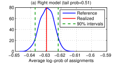
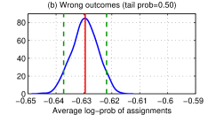
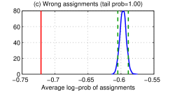
(a) Results of the assignment test. Model (c), which has a wrong assignment mechanism, fails the test. The plots for the fiction scenario (not shown) are similar to these ones, as the assignments are assumed independent of the outcomes.

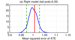
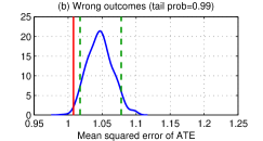
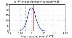
(b) Results of the outcome test. The test fails for the model in which the outcome model is misspecified.

Figure 1: Results of the tests for the science-fiction scenario, in which we have access to both counterfactual outcomes.

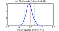
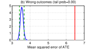
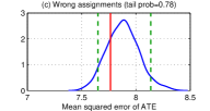
(a) Our approach.

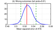
(b) Gelman et al., (2005).

Figure 2: Results of the outcome tests for the fiction scenario, in which we only observe one counterfactual outcome. (a) The outcome test fails for the model in which the outcome model is misspecified. (b) If we impute the missing data following Gelman et al., (2005), the test does not fail, although we are using the wrong outcome model.

4 Empirical Study

We use both synthetic and real data to illustrate how to validate causal models. With synthetic data we compare our conclusions to the true data generating mechanism. With real data we demonstrate our approach to criticize causal models in practice. In all our studies, we apply the discrepancies from Section 3.2; Section 3.3, i.e., the marginal log-likelihood of the assignments (Eq.7) and the mean squared error of the average treatment effect (Eq.10). Note we focus here on the insights of the criticisms and not the insights of the causal inferences.

4.1 Synthetic data

We showcase the results of different predictive checks using data generated from a linear model (detailed below). We first perform inference under the correct model specification. Then we introduce misspecifications, either on the outcome model or the assignment model.

We generate $10,000$ data points, each with a $10$-dimensional covariate $x_{i}$, a binary treatment $a_{i}$, and a set of potential outcomes $(y_{i}(0),y_{i}(1))$,

$$x_{i}\sim\textrm{Uniform}(x_{i}\,|\,[0,1]^{10}),$$

$$a_{i}\,|\,x_{i}\sim\textrm{Bernoulli}\left(a_{i}\,|\,\textrm{logistic}(x_{i}^{\top}\phi)\right),$$

$$y_{i}(a)\,|\,x_{i}\sim\mathcal{N}\left(y_{i}(a)\,|\,[x_{i},a]^{\top}\theta,\sigma^{2}\right),$$

We place a standard normal prior over the parameters $\phi$, $\theta$, and a gamma prior with unit shape and rate on $\sigma^{2}$.

We study two scenarios: (i) In the “science-fiction” scenario, we have access simultaneously to $y_{i}(0)$ and $y_{i}(1)$. (This is not possible in the real world.) (ii) In the “fiction” scenario, we only have access to one counterfactual outcome, $y_{i}=a_{i}y_{i}(1)+(1-a_{i})y_{i}(0)$, and there are no hidden confounders. In each scenario, we check three causal models: (a) the correct model as specified above; (b) a “wrong outcomes” model, where we misspecify the distribution over $y_{i}(a)$ by ignoring the first entry of $x_{i}$ (i.e., $\theta_{1}=0$); (c) a “wrong assignment” model, where we misspecify the distribution over $a_{i}$ by setting the probability that $a_{i}=1$ to $(0.7+0.3\times\textrm{logistic}(x_{i}^{\top}\phi))$.

We approximate the posterior with Markov chain Monte Carlo in Stan (Carpenter et al.,, 2016), obtaining $1000$ samples. In the fiction scenario, we weigh the observations to form the outcome discrepancy (Section 3). In the science-fiction scenario, we do not weigh the observations because we see both $y(0)$ and $y(1)$.

Figure 1(a) illustrates criticism of the assignment model (Eq.7) for the science-fiction scenario. (The plots for the fiction scenario are similar.) As expected, when we use the correct model the realized discrepancy is approximately in the center of the reference distribution (panel a); this indicates that the model is correctly specified. We see the same for the misspecified outcome model (panel b) because the assignment mechanism is still correct. However, when the assignment model is wrong, the realized discrepancy against the reference distribution (panel c) suggests that the model is misspecified.

We now turn to criticizing the outcome model. Figure 1(b); Figure 2(a) illustrate the test of the mean squared error of the average treatment effect (ate) (Eq.10) for the science-fiction and fiction scenarios, respectively. As expected, the test for the correct model does not suggest any issue (panel a). When the outcome model is wrong, the test fails (panel b). This correctly indicates that we should revise the model. In the science-fiction scenario, the misspecification on the assignment model does not affect the outcome model (panel c), and thus the test indicates correctness.

In the fiction scenario, our test for the outcome model indicates correctness. In general, however, the outcome test may fail if the assignment model is misspecified because it affects the inverse propensity weighting.

Finally, Figure 2(b) shows the outcome test when we impute the missing data following Gelman et al., (2005). The bias leads the test to pass (see Section 3), even though we use the misspecified outcome model.

4.2 Observational study: Cockroaches

We analyze a real observational study of the effect of pest management on cockroach levels in urban apartments (Gelman and Hill,, 2006). Each apartment $i$ was set up with traps for several days. The response is the number of cockroaches trapped during that period; the treatment corresponds to having applied the pesticide. We expect the pesticide to reduce the number of cockroaches.

Let $t_{i}$ be the number of trap days and $y_{i}$ the number of cockroaches for each apartment. We use two additional covariates: the pre-treatment roach level $r_{i}$ and an indicator $s_{i}$ of whether the apartment is a “senior” building, restricted to the elderly. We model the data as Poisson,

$$y_{i}\,|\,a_{i},x_{i}\sim\textrm{Poisson}\left(y_{i}\,|\,\mu_{i}\right),$$

where $\mu_{i}=t_{i}\exp\left\{\theta_{0}+\theta_{1}s_{i}+\theta_{2}r_{i}+\theta_{3}a_{i}\right\}$, $a_{i}$ is the treatment indicator, $\theta$ is the outcome model parameter, and $x_{i}=\{t_{i},s_{i},r_{i}\}$. We posit a logistic assignment model,

$$a_{i}\,|\,x_{i}\sim\textrm{Bernoulli}\left(a_{i}\,|\,\textrm{logistic}([1,s_{i},r_{i}]^{\top}\phi)\right).$$

We place standard normal priors over the parameters and draw $1000$ posterior samples.

We first evaluate the assignment model with the average log-likelihood of the assignments. Figure 3(a) illustrates the test. The realized discrepancy is plausible.

Next we evaluate the outcome model, again with the mean squared error of the ate. Figure 3(b) (left) illustrates the outcome test for the Poisson model. The test fails: the model lacks the overdispersion needed to capture the high variance of the data (Gelman and Hill,, 2006). This is typical with the Poisson because its variance is equal to its mean.

We propose two alternative models. Model (b) replaces the Poisson likelihood with a negative binomial distribution. It has the same mean $\mu_{i}$ as the Poisson but its variance increases quadratically. The variance is $\mu_{i}+\mu_{i}^{2}/\theta_{4}$, where $\theta_{4}$ is a dispersion parameter. We place a gamma prior with unit shape and rate over $\theta_{4}$. Model (c) has similar considerations, but the variance is now a linear function of the mean $\theta_{4}\mu_{i}$. Figure 3(b) (center and right) illustrates the causal tests for models (b) and (c). These results suggest that model (c) is the most plausible.

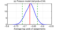
(a) Assignment test.

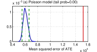
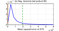
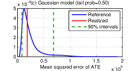
(b) Outcome test.

Figure 3: Results for the cockroaches infestation study. The assignment test does not suggest any assignment model flaw. The outcome tests suggest that the variance is a linear function of the mean.

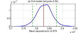
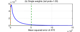
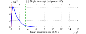
Figure 4: Results of the outcome test for the television show study. The models with a single weight for all grades (b) or a single intercept for all pairs (c) are too simple and fail the test.

4.3 Randomized experiment: The Electric Company television show

We now consider an educational experiment performed around 1970 on a set of elementary school classes. The treatment in this experiment was exposure to a new educational television show called The Electric Company. In each of four grades, the classes were completely randomized into treated and control groups. At the end of the school year, students in all the classes were given a reading test, and the average test score within each class was recorded. The data are at the classroom level.

Two classes from each grade were selected from each school. Let $y_{i1}$ and $y_{i2}$ be the scores of each class for the treatment and control groups, respectively. Let $p_{i1}$ and $p_{i2}$ be their pre-treatment scores at the beginning of the year. We also introduce the notation $g(i)$ to denote the grade (from 1 to 4) of the two classes from the $i$-th pair. We first use a regression model of the form

$$y_{i1}\sim\mathcal{N}(y_{i1}\,|\,b_{i}+m_{g(i)}p_{i1}+\theta_{g(i)},\sigma_{g(i)}^{2}),$$

$$y_{i2}\sim\mathcal{N}(y_{i2}\,|\,b_{i}+m_{g(i)}p_{i2},\sigma_{g(i)}^{2}),$$

where the model parameters are: $b_{i}$, the intercept term that depends on the specific pair $i$; $m_{1:4}$, the weight of $p_{i1}$ for each grade; $\theta_{1:4}$, the treatment effect; and $\sigma^{2}_{1:4}$, the variance for each grade. We place a Gaussian prior over the intercepts $b_{i}\sim\mathcal{N}(\mu_{g(i)},\tau_{g(i)}^{2})$. We also place Gaussian priors with zero mean and variance $10^{4}$ over $\mu_{g}$, $\theta_{g}$, and $m_{g}$. We place gamma priors with shape $10$ and rate $1$ over $\sigma_{g}$ and $\tau_{g}$. We refer to this model as model (a). We also test two simplified models. Model (b) assumes that the parameters $\theta$ and $m$ do not depend on the specific grade. Model (c) assumes instead that the intercept $b$ is shared for all pairs. Since we know that this is a completely randomized experiment by design, we do not posit any assignment model.

We plot in Figure 4 the results of the outcome test, which is based on the mean squared error of the average treatment effect. Model (a), which is the most flexible, seems to provide a sensible fit of the data. However, models (b) and (c) are too simplistic. They clearly fail the test. If we had started from any of these models in our analysis, the test would suggest the need to revise them.

5 Discussion

We have developed model criticism for Bayesian causal inference. This provides a rigorous foundation for diagnosing if a given probabilistic model is appropriate.

Here, we assume the typical setup in Bayesian causal inference in which the posterior factorizes across outcome and assignment parameters. However, this can lead to poor frequentist properties (Robins and Ritov,, 1997; Robins,, 2004). To accommodate this, Bayesian-frequentist compromises have been proposed which force dependency between the outcome and assignment models (Hoshino,, 2008; McCandless et al.,, 2009; Graham et al.,, 2016). In future work, we will study causal discrepancies which are of the general form of Eq.5, i.e., which depend simultaneously on assignments and potential outcomes. Such discrepancies could also be applied to check causal models with a non-ignorable assignment mechanism.

Finally, there has been a surge of interest in model-based causal inference for high-dimensional, massive, and heterogenous data. In such settings, one can capture more fine-grained phenomena, whether it be with hierarchical models (Hirano et al.,, 2000; Feller and Gelman,, 2014), regularized regressions (Maathuis et al.,, 2009; Belloni et al.,, 2014), structural equation models (Bottou et al.,, 2013; Peters et al.,, 2015), or neural networks (Johansson et al.,, 2016). This is an important regime for checking causal models.

References

Appendix A Notation

We provide a table describing the notation we use in this paper. See Table 1; Table 2; Table 3.

Symbol	Description
$A_{i}$	Treatment assignment of individual $i$ (random variable)
$Y_{i}(0),Y_{i}(1)$	Potential outcomes of individual $i$ (random variable)
$\boldsymbol{\mathbf{A}}=(A_{1},\ldots,A_{n})^{\top}$	Set of treatment assignments (random variable)
$\boldsymbol{\mathbf{Y}}(0),\boldsymbol{\mathbf{Y}}(1)$	Set of potential outcomes (random variable)
$=(Y_{1}(0),\ldots,Y_{n}(0))^{\top},(Y_{1}(1),\ldots,Y_{n}(1))^{\top}$
$a_{i}$	Treatment assignment of individual $i$
$y_{i}(a_{i})$	Outcome of individual $i$ when assigned to treatment $a_{i}$
$x_{i}$	Observed covariates of individual $i$
$\boldsymbol{\mathbf{a}}$	Set of treatment assignments
$\boldsymbol{\mathbf{y}}(0),\boldsymbol{\mathbf{y}}(1)$	Set of potential outcomes
$\boldsymbol{\mathbf{y}}(\boldsymbol{\mathbf{a}})=(y_{1}(a_{1}),\ldots,y_{n}(a_{n}))^{\top}$	Set of outcomes when assigned to set of treatments
$\boldsymbol{\mathbf{x}}$	Set of observed covariates
$\mathcal{D}^{\rm obs}=\{a_{i},y_{i}(a_{i})\}$	Observed data set
$\mathcal{D}^{\rm do}=\{a_{i}^{\rm do},y_{i}(a_{i}^{\rm do})\}$	Hypothetical data set from an intervention

Table 1: Notation for observational data.

Symbol	Description
$\boldsymbol{\mathbf{\phi}}$	Parameters of the assignment model
$p(a_{i}\,|\,x_{i},\boldsymbol{\mathbf{\phi}})$	Assignment likelihood for individual $i$
$p(\boldsymbol{\mathbf{a}}\,|\,\boldsymbol{\mathbf{x}},\boldsymbol{\mathbf{\phi}})=\prod_{i=1}^{n}p(a_{i}\,|\,x_{i},\boldsymbol{\mathbf{\phi}})$	Assignment likelihood
$p(\boldsymbol{\mathbf{a}}\,|\,\boldsymbol{\mathbf{x}},\boldsymbol{\mathbf{\phi}})p(\boldsymbol{\mathbf{\phi}})$	Assignment model
$\boldsymbol{\mathbf{\theta}}$	Parameters of the outcome model
$p(y_{i}(0),y_{i}(1)\,|\,x_{i},\boldsymbol{\mathbf{\theta}})$	Outcome likelihood for individual $i$
$p(\boldsymbol{\mathbf{y}}(0),\boldsymbol{\mathbf{y}}(1)\,|\,\boldsymbol{\mathbf{x}},\boldsymbol{\mathbf{\theta}})=\prod_{i=1}^{n}p(y_{i}(0),y_{i}(1)\,|\,x_{i},\boldsymbol{\mathbf{\theta}})$	Outcome likelihood
$p(\boldsymbol{\mathbf{y}}(0),\boldsymbol{\mathbf{y}}(1)\,|\,\boldsymbol{\mathbf{x}},\boldsymbol{\mathbf{\theta}})p(\boldsymbol{\mathbf{\theta}})$	Outcome model
$p(\boldsymbol{\mathbf{y}}(0),\boldsymbol{\mathbf{y}}(1)\,|\,\boldsymbol{\mathbf{x}},\boldsymbol{\mathbf{\theta}})p(\boldsymbol{\mathbf{\theta}})p(\boldsymbol{\mathbf{a}}\,|\,\boldsymbol{\mathbf{x}},\boldsymbol{\mathbf{\phi}})p(\boldsymbol{\mathbf{\phi}})$	Causal model
$p(\boldsymbol{\mathbf{a}}^{\rm rep}\,|\,\boldsymbol{\mathbf{x}},\boldsymbol{\mathbf{\phi}})p(\boldsymbol{\mathbf{\phi}}\,|\,\boldsymbol{\mathbf{a}})$	Assignment model (a posteriori)
$p(\boldsymbol{\mathbf{y}}(0)^{\rm rep},\boldsymbol{\mathbf{y}}(1)^{\rm rep}\,|\,\boldsymbol{\mathbf{x}},\boldsymbol{\mathbf{\theta}})p(\boldsymbol{\mathbf{\theta}}\,|\,\boldsymbol{\mathbf{y}})$	Outcome model (a posteriori)
$p(\boldsymbol{\mathbf{y}}(0)^{\rm rep},\boldsymbol{\mathbf{y}}(1)^{\rm rep}\,|\,\boldsymbol{\mathbf{x}},\boldsymbol{\mathbf{\theta}})p(\boldsymbol{\mathbf{\theta}}\,|\,\boldsymbol{\mathbf{y}})p(\boldsymbol{\mathbf{a}}^{\rm rep}\,|\,\boldsymbol{\mathbf{x}},\boldsymbol{\mathbf{\phi}})p(\boldsymbol{\mathbf{\phi}}\,|\,\boldsymbol{\mathbf{a}})$	Causal model (a posteriori)

Table 2: Notation for causal models.

Symbol	Description
$(\boldsymbol{\mathbf{y}}(0)^{\rm rep},\boldsymbol{\mathbf{y}}(1)^{\rm rep}),\boldsymbol{\mathbf{a}}^{\rm rep}$	Replicated data set of outcomes and assignments
$T((\boldsymbol{\mathbf{y}}(0),\boldsymbol{\mathbf{y}}(1)),\boldsymbol{\mathbf{a}},\boldsymbol{\mathbf{\theta}},\boldsymbol{\mathbf{\phi}})$	Causal discrepancy (over realizations)
$T^{\rm rep,s}=T((\boldsymbol{\mathbf{y}}(0)^{{\rm rep},s},\boldsymbol{\mathbf{y}}(1)^{{\rm rep},s}),\boldsymbol{\mathbf{a}}^{\rm rep},\boldsymbol{\mathbf{\theta}}^{s},\boldsymbol{\mathbf{\phi}}^{s})$	Discrepancy over replication $s$
$T^{\rm obs,s}=T((\boldsymbol{\mathbf{y}}(0),\boldsymbol{\mathbf{y}}(1)),\boldsymbol{\mathbf{a}},\boldsymbol{\mathbf{\theta}}^{s},\boldsymbol{\mathbf{\phi}}^{s})$	Realized discrepancy over replication $s$
$p(T)=\{T^{\rm rep,s}\}$	Reference distribution
$T^{\rm obs}=\{T^{\rm obs,s}\}$	Realized discrepancy

Table 3: Notation for model criticism.

References

- Angrist, (2004) Angrist, J. D. (2004). Treatment effect heterogeneity in theory and practice. The Economic Journal, 114(494):C52–C83.
- Athey and Imbens, (2015) Athey, S. and Imbens, G. (2015). Machine learning methods for estimating heterogeneous causal effects. arXiv preprint arXiv:1504.01132.
- Austin, (2009) Austin, P. C. (2009). Balance diagnostics for comparing the distribution of baseline covariates between treatment groups in propensity-score matched samples. Statistics in medicine, 28(25):3083–3107.
- Bang and Robins, (2005) Bang, H. and Robins, J. M. (2005). Doubly robust estimation in missing data and causal inference models. Biometrics, 61(4):962–972.
- Bayarri et al., (2007) Bayarri, M., Castellanos, M., et al. (2007). Bayesian checking of the second levels of hierarchical models. Statistical Science, 22(3):322–343.
- Belloni et al., (2014) Belloni, A., Chernozhukov, V., and Hansen, C. (2014). Inference on treatment effects after selection among high-dimensional controls. The Review of Economic Studies, 81(2):608–650.
- Bottou et al., (2013) Bottou, L., Peters, J., Quiñonero-Candela, J., Charles, D. X., Chickering, D. M., Portugaly, E., Ray, D., Simard, P., and Snelson, E. (2013). Counterfactual reasoning and learning systems: the example of computational advertising. The Journal of Machine Learning Research, 14:3207–3260.
- Box, (1980) Box, G. E. P. (1980). Sampling and Bayes’ inference in scientific modelling and robustness. Journal of the Royal Statistical Society. Series A. General, 143(4):383–430.
- Carpenter et al., (2016) Carpenter, B., Gelman, A., Hoffman, M., Lee, D., Goodrich, B., Betancourt, M., Brubaker, M. A., Guo, J., Li, P., and Riddell, A. (2016). Stan: A probabilistic programming language. Journal of Statistical Software.
- Chaloner, (1991) Chaloner, K. (1991). Bayesian residual analysis in the presence of censoring. Biometrika, 78(3):637–644.
- Chen and Pearl, (2015) Chen, B. and Pearl, J. (2015). Exogeneity and robustness. Technical report.
- Dawid and Dickey, (1977) Dawid, A. and Dickey, J. M. (1977). Likelihood and bayesian inference from selectively reported data. Journal of the American Statistical Association, 72(360a):845–850.
- Dawid, (1984) Dawid, A. P. (1984). Present position and potential developments: Some personal views: Statistical theory: The prequential approach. Journal of the Royal Statistical Society. Series A (General), pages 278–292.
- Dehejia, (2005) Dehejia, R. (2005). Practical propensity score matching: a reply to smith and todd. Journal of econometrics, 125(1):355–364.
- Dehejia and Wahba, (2002) Dehejia, R. H. and Wahba, S. (2002). Propensity score-matching methods for nonexperimental causal studies. Review of Economics and statistics, 84(1):151–161.
- Feller and Gelman, (2014) Feller, A. and Gelman, A. (2014). Hierarchical Models for Causal Effects. An Interdisciplinary, Searchable, and Linkable Resource. John Wiley & Sons, Inc., Hoboken, NJ, USA.
- Gelman and Hill, (2006) Gelman, A. and Hill, J. L. (2006). Data Analysis Using Regression and Multilevel/Hierarchical Models. Cambridge University Press.
- Gelman et al., (1996) Gelman, A., Meng, X.-L., and Stern, H. (1996). Posterior predictive assessment of model fitness via realized discrepancies. Statistica Sinica, 6(4):733–760.
- Gelman and Shalizi, (2012) Gelman, A. and Shalizi, C. R. (2012). Philosophy and the practice of Bayesian statistics. British Journal of Mathematical and Statistical Psychology, 66(1):8–38.
- Gelman et al., (2005) Gelman, A., Van Mechelen, I., Verbeke, G., Heitjan, D. F., and Meulders, M. (2005). Multiple imputation for model checking: Completed-data plots with missing and latent data. Biometrics, 61(1):74–85.
- Graham et al., (2016) Graham, D. J., McCoy, E. J., Stephens, D. A., et al. (2016). Approximate bayesian inference for doubly robust estimation. Bayesian Analysis, 11(1):47–69.
- Greene, (2003) Greene, W. H. (2003). Econometric analysis. Pearson Education India.
- Heckman and Hotz, (1989) Heckman, J. J. and Hotz, V. J. (1989). Choosing among alternative nonexperimental methods for estimating the impact of social programs: The case of manpower training. Journal of the American Statistical Association, 84(408):862–874.
- Heckman et al., (1998) Heckman, J. J., Ichimura, H., and Todd, P. (1998). Matching as an econometric evaluation estimator. The Review of Economic Studies, 65(2):261–294.
- Hirano et al., (2000) Hirano, K., Imbens, G. W., Rubin, D. B., and Zhou, X.-H. (2000). Assessing the effect of an influenza vaccine in an encouragement design. Biostatistics, 1(1):69–88.
- Holland, (1986) Holland, P. W. (1986). Statistics and causal inference. Journal of the American Stat. Association.
- Hoshino, (2008) Hoshino, T. (2008). A Bayesian propensity score adjustment for latent variable modeling and mcmc algorithm. Computational Statistics & Data Analysis, 52(3):1413–1429.
- Imbens and Rubin, (2015) Imbens, G. and Rubin, D. B. (2015). Causal Inference. Cambridge University Press.
- Johansson et al., (2016) Johansson, F. D., Shalit, U., and Sontag, D. (2016). Learning Representations for Counterfactual Inference. In International Conference on Machine Learning.
- Little and Rubin, (1987) Little, R. J. and Rubin, D. B. (1987). Statistical analysis with missing data. John Wiley & Sons.
- Lu and White, (2014) Lu, X. and White, H. (2014). Robustness checks and robustness tests in applied economics. Journal of Econometrics, 178:194–206.
- Maathuis et al., (2009) Maathuis, M. H., Kalisch, M., Bühlmann, P., et al. (2009). Estimating high-dimensional intervention effects from observational data. The Annals of Statistics, 37(6A):3133–3164.
- McCandless et al., (2009) McCandless, L. C., Gustafson, P., and Austin, P. C. (2009). Bayesian propensity score analysis for observational data. Statistics in Medicine, 28(1):94–112.
- Meng, (1994) Meng, X.-L. (1994). Posterior predictive p-values. The Annals of Statistics, pages 1–19.
- Mimno and Blei, (2011) Mimno, D. and Blei, D. M. (2011). Bayesian checking of topic models. In Empirical Methods on Natural Language Processing.
- Mimno et al., (2015) Mimno, D., Blei, D. M., and Engelhardt, B. (2015). Posterior predictive checks to quantify lack-of-fit in admixture models of latent population structure. Proceedings of the National Academy of Sciences, 112(26).
- Morgan and Winship, (2014) Morgan, S. L. and Winship, C. (2014). Counterfactuals and causal inference. Cambridge University Press.
- Neyman, (1923) Neyman, J. (1923). On the application of probability theory to agricul- tural experiments. essay on principles. section 9. Roczniki Nauk Rolniczych Tom X.
- Pearl, (2000) Pearl, J. (2000). Causality. Cambridge University Press.
- Peters et al., (2015) Peters, J., Bühlmann, P., and Meinshausen, N. (2015). Causal inference using invariant prediction: identification and confidence intervals. arXiv preprint arXiv:1501.01332.
- Raudenbush and Bryk, (1986) Raudenbush, S. and Bryk, A. S. (1986). A hierarchical model for studying school effects. Sociology of education, pages 1–17.
- Robins, (2004) Robins, J. M. (2004). Optimal structural nested models for optimal sequential decisions. In Proceedings of the second seattle Symposium in Biostatistics, pages 189–326. Springer.
- Robins et al., (2000) Robins, J. M., Hernan, M. A., and Brumback, B. (2000). Marginal structural models and causal inference in epidemiology. Epidemiology, pages 550–560.
- Robins and Ritov, (1997) Robins, J. M. and Ritov, Y. (1997). Toward a curse of dimensionality appropriate(coda) asymptotic theory for semi-parametric models. Statistics in Medicine, 16(3):285–319.
- Robins and Rotnitzky, (2001) Robins, J. M. and Rotnitzky, A. (2001). Comments. Statistica Sinica, pages 920–936.
- Rosenbaum et al., (1987) Rosenbaum, P. R. et al. (1987). The role of a second control group in an observational study. Statistical Science, 2(3):292–306.
- Rosenbaum and Rubin, (1983) Rosenbaum, P. R. and Rubin, D. B. (1983). The central role of the propensity score in observational studies for causal effects. Biometrika, 70(1):41–55.
- Royle and Dorazio, (2008) Royle, J. A. and Dorazio, R. M. (2008). Hierarchical modeling and inference in ecology: the analysis of data from populations, metapopulations and communities. Academic Press.
- Rubin, (1974) Rubin, D. B. (1974). Estimating causal effects of treatments in randomized and nonrandomized studies. Journal of Educational Psychology, 66(5):688.
- Rubin, (1976) Rubin, D. B. (1976). Inference and missing data. Biometrika, 63(3):581–592.
- Rubin, (1984) Rubin, D. B. (1984). Bayesianly justifiable and relevant frequency calculations for the applied statistician. The Annals of Statistics, 12(4):1151–1172.
- Rubin, (2008) Rubin, D. B. (2008). For objective causal inference, design trumps analysis. The Annals of Applied Statistics, 2(3):808–840.
- Su et al., (2011) Su, Y.-S., Gelman, A., Hill, J., Yajima, M., et al. (2011). Multiple imputation with diagnostics (mi) in r: Opening windows into the black box. Journal of Statistical Software, 45(2):1–31.
- Van der Laan et al., (2007) Van der Laan, M. J., Polley, E. C., and Hubbard, A. E. (2007). Super learner. Statistical applications in genetics and molecular biology, 6(1).
- Van der Laan and Robins, (2003) Van der Laan, M. J. and Robins, J. M. (2003). Unified methods for censored longitudinal data and causality. Springer Science & Business Media.
- Van der Laan and Rubin, (2006) Van der Laan, M. J. and Rubin, D. (2006). Targeted maximum likelihood learning. The International Journal of Biostatistics, 2(1).
- Wooldridge, (2010) Wooldridge, J. M. (2010). Econometric analysis of cross section and panel data. MIT press.
- Yano et al., (2001) Yano, Y., Beal, S. L., and Sheiner, L. B. (2001). Evaluating pharmacokinetic/pharmacodynamic models using the posterior predictive check. Journal of pharmacokinetics and pharmacodynamics, 28(2):171–192.