Analysis of random walks on a hexagonal lattice

Abstract

We consider a discrete-time random walk on the nodes of an unbounded hexagonal lattice. We determine the probability generating functions, the transition probabilities and the relevant moments. The convergence of the stochastic process to a 2-dimensional Brownian motion is also discussed. Furthermore, we obtain some results on its asymptotic behavior making use of large deviation theory. Finally, we investigate the first-passage-time problem of the random walk through a vertical straight-line. Under suitable symmetry assumptions we are able to determine the first-passage-time probabilities in a closed form, which deserve interest in applied fields. Random walk; Hexagonal lattice; Probability generating function; Large deviations; Moderate deviations; First-passage time.
2000 Math Subject Classification: 60J15; 60F10; 82C41

1 Introduction

Stimulated by potential applications in many fields of science and engineering, in this paper we aim to study a discrete-time random walk on the nodes of an unbounded hexagonal lattice. Specific properties of this kind of structures make them attractive for various applications, such as thermal isolation, energy absorption, and structural protection. For a more detailed description on the use of honeycomb structures in applied fields see Haghpanah et al. (2013). Some general results on discrete-time random walks on a lattice can be found in Montroll (1964), Montroll and Weiss (1965) and in Lawler and Limic (2010). See also the investigation of Guillotin-Plantard (2005) concerning random walks on regular graphs, and the recent review by Masuda et al. (2017).

Our attention focuses on certain mathematical properties of the stochastic process under investigation, where the underlying lattice state-space is a general honeycomb structure (the hexagonal lattice). Specifically, we give emphasis on the transient distribution of the random walk. We also study its asymptotic behavior making use of the theory of large deviations. In view of the relevance in several applied contexts, our efforts are finally oriented to the determination of the first-passage-time probabilities of the random walk through suitable straight-line boundaries.

Two-dimensional random walk models on hexagonal structures deserve interest in various applied fields, such as Biomathematics, Cellular networks, Physics, and Chemical models.

A correlated random walk on a hexagonal lattice has been used by Prasad and Borges (2006) in order to determine the optimal movement strategy of an animal searching for resources upon a network of patches. Moreover, hexagonal lattices have been adopted to characterize landscapes in suitable spatial models of bird populations, since hexagons allow better packing of territories in space, see Pulliam et al. (1992). In Personal Communications Services networks, such as the honeycomb Poisson-Voronoi access cellular network model, the movement of mobile users may be captured by random walks models on the hexagonal lattice (cf.  Akyildiz et al. (2000), Baccelli and Blaszczyszyn (2009)). We remark that the above mentioned investigations deal with random walks among adjacent cells.

Other types of processes dealing with two-dimensional random walks on hexagonal structures are employed to study: the behavior of cracks among frozen regions in a dimer model (cf.  Boutillier (2007)), the representation of the correlation functions in valence-bond solid models (cf.  Kennedy et al. (1988)), the light transport in a honeycomb structure (cf.  Miri and Stark (2003)), electronic properties of deformed carbon nanotubes (cf.  Schuyler et al. (2005)), and the incoherent energy transfer due to long range interactions in two-dimensional regular systems (cf.  Zumofen and Blumen (1982)).

A mathematical model based on a three-axes description of the honeycomb lattice has been proposed by Cotfas (2000), where the movement of an excitation (or a vacancy) on a quasicrystal is regarded as a suitable random walk. A random-walk model of absorption of an isolated polymer chain on various lattice models, including the hexagonal one, is investigated in Rubin (1965). Moreover, as a model of polymer dynamics, Sokolov et al. (1993) analyzed the continuous-time motion of a rigid equilateral triangle in the plane, where the center of mass of the triangle performs a random walk on the vertices of the hexagonal lattice.

Our study is first finalized to obtain a closed-form result of the probability generating function and of the probability distribution of the random walk on the hexagonal lattice. This is performed by considering a partition of the state space into two sets, i.e. the states visited at even and odd times. Then, the iterative equations of the relevant probabilities for the two sets are expressed in a suitable way. A similar approach has been used by Di Crescenzo et al. (2014) for the analysis of random walks in continuous time characterized by alternating rates. Some auxiliary results are also obtained, such as certain symmetry properties of the state probabilities and the relevant moments, including the covariance. The validity of a customary convergence to a 2-dimensional Brownian motion is also shown. Differently from previous investigations oriented to computing numerical quantities of interest, such as critical exponents (see de Forcrand et al. (1986), for instance), our approach is mainly theoretical. Indeed, we remark that our study leads to closed-form results even in the general case of non-constant one-step transition probabilities. For general results on other types of discrete-time random walks see the contributions by Katzenbeisser and Panny (2002), Böhm and Hornik (2010) and Panny and Prodinger (2016).

Our second aim is to investigate two different forms of asymptotic behavior of the random walk on the hexagonal lattice, by making use of some applications of the Gärtner Ellis Theorem. About this topic we recall the text by Feng and Kurtz (2006) for a wide study on sample path large deviations for general Markov processes. It is worth pointing out that our results concerning the large deviation principle (LDP for short) can be used to evaluate some quantities of interest in applied contexts, such as estimates of hitting probabilities that are relevant for Monte Carlo simulation through the importance sampling technique (see, for instance, the overview in Blanchet and Lam (2012), or Section 5 and 6 of Asmussen and Glynn (2007), and Collamore (2002).)

In conclusion, we also face the first-passage-time problem of the considered random walk through straight-line boundaries. We first investigate the “taboo probability” concerning transitions on the nodes of the hexagonal lattice that avoid the boundary. Suitable symmetry conditions allow us to obtain closed-form expressions of such taboo probabilities and, in turn, of the corresponding first-passage-time probabilities. An example of the usefulness of these results in the context of polymer science is provided at the end of Section 5. We note that obtaining closed-form expressions for random walks on lattices generally is not an easy task.

Here is the plan of the paper: The main definitions and the description of the process are given in Section 2. The probability distribution of the random walk, with the generating function and the main moments are obtained in Section 3. Section 4 is devoted to investigation of the large and moderate deviations. In Section 5 we analyze the first-passage-time problem of the random walk through straight-line boundaries. Finally, in Section 6 we provide some concluding remarks.

2 The Random Walk Model

We consider the hexagonal lattice on a reference system of cartesian axes, taking a vertex of a generic hexagon as the origin of the reference system, as shown in Fig. 1. Since the considered structure consists of hexagonal cells, with angles of $2\pi/3$, we can assume that the distance between two generic adjacent vertices is a constant, say $a$. Hence, the coordinates of the vertices are repeated regularly. We divide the vertices into two categories:

$$\mathscr{V}_{i}=\left\{\left(\frac{3}{2}aj+ia;\;\frac{\sqrt{3}}{2}aj+\sqrt{3}ak\right);\;j,k\in\mathbb{Z}\right\},\quad i=0,1.$$ (1)

Figure 1: Graphical representation of the hexagonal lattice, where the vertices of $\mathscr{V}_{0}$ $(\mathscr{V}_{1})$ are represented by white (black) circles.

Figure 2: One-step transition probabilities.

With reference to Fig. 1, we consider a random walk of a particle that starts at a vertex with coordinates $(x,y)$ and it moves to an adjacent vertex following an appropriate transition probability. In particular, as shown in Fig. 2, if the particle is located in a vertex of the set $\mathscr{V}_{0}$, it can reach the three adjacent positions with probabilities $q_{0,0}$, $q_{0,1}$, $q_{0,2}$ and then the particle will occupy a vertex of $\mathscr{V}_{1}$. Similarly, if the particle is in a vertex of $\mathscr{V}_{1}$, in one step it reaches one of the three adjacent positions, belonging to $\mathscr{V}_{0}$, with probabilities $q_{1,0}$, $q_{1,1}$, $q_{1,2}$ (see Fig. 2). We remark that the hexagonal graph is a bipartite graph, this property being useful for the evaluation of the results of Section 3.

Let $\{(X_{n},Y_{n}),n\in\mathbb{N}_{0}\}$ be the discrete-time random walk having state space $\mathscr{V}_{0}\cup\mathscr{V}_{1}$ and representing the position of the particle at time $n$. From the above notations, for $i=0,1$ and $r=0,1,2$ the one-step transition probabilities are expressed as

$$q_{i,r}=\mathbb{P}\left[\binom{X_{n+1}}{Y_{n+1}}=\binom{x+a\cos\left(r\frac{2}{3}\pi+i\pi\right)}{y+a\sin\left(r\frac{2}{3}\pi+i\pi\right)}\left|\binom{X_{n}}{Y_{n}}=\binom{x}{y}\right.\right],$$ (2)

with

$$\sum_{r=0}^{2}q_{i,r}=1,\qquad i=0,1.$$

Let us now introduce the state probabilities at time $n$, $n\in\mathbb{N}_{0}$,

$$p_{j,k}(n):=\mathbb{P}\left[(X_{n},Y_{n})=\left(\frac{3}{2}aj+i_{n}a,\frac{\sqrt{3}}{2}aj+\sqrt{3}ak\right)\right],\quad j,k\in\mathbb{Z},$$ (3)

where

$$i_{n}=\frac{1}{2}\left(1-(-1)^{n}\right).$$ (4)

We assume that $\mathbb{P}[(X_{0},Y_{0})=(0,0)]=1$, so that the initial condition reads

$$p_{0,0}(0)=1.$$ (5)

Hence, from the previous assumptions, and noting that at even (odd) times the particle occupies states of set $\mathscr{V}_{0}$ ($\mathscr{V}_{1}$), the forward Kolmogorov equations for the state probabilities, for all $n\in\mathbb{N}_{0}$ are given by

$$p_{j,k}(n+1)=\left\{\begin{array}[]{ll}p_{j,k}(n)q_{0,0}+p_{j+1,k}(n)q_{0,2}+p_{j+1,k-1}(n)q_{0,1},&n\hbox{ even}\\[5.69054pt] p_{j,k}(n)q_{1,0}+p_{j-1,k+1}(n)q_{1,1}+p_{j-1,k-1}(n)q_{1,2},&n\hbox{ odd}\end{array}\right.$$ (6)

with initial condition (5).

3 Probability Distribution

Now we focus on the probability generating function $G(u,v;n)$ of $(X_{n},Y_{n})$. Due to (3), it is defined by

$$G(u,v;n)=\mathbb{E}\left[u^{X_{n}}v^{Y_{n}}\right]=\sum_{j\in\mathbb{Z}}u^{\frac{3}{2}aj+i_{n}a}\sum_{k\in\mathbb{Z}}v^{\frac{\sqrt{3}}{2}aj+\sqrt{3}ak}p_{j,k}(n),$$ (7)

for $u>0$ and $v>0$.

Proposition 3.1.

The explicit expression of the probability generating function $G(u,v;n)$ of $(X_{n},Y_{n})$, for $n\in\mathbb{N}_{0}$, $u>0$ and $v>0$ is:

$$G(u,v;n)=F_{i_{n}}(\tilde{u},\tilde{v};n)u^{i_{n}a},$$ (8)

where $i_{n}$ is defined by (4), with

$$\tilde{u}=u^{\frac{3}{2}a}v^{\frac{\sqrt{3}}{2}a},\qquad\tilde{v}=v^{\sqrt{3}a},$$ (9)

and

$$F_{i_{n}}(u,v;n)=\left(q_{1,0}+q_{1,2}u+q_{1,1}\frac{u}{v}\right)^{\frac{n}{2}-\frac{1}{2}{i_{n}}}\left(q_{0,0}+q_{0,1}\frac{v}{u}+q_{0,2}\frac{1}{u}\right)^{\frac{n}{2}+\frac{1}{2}{i_{n}}}.$$ (10)

Proof 3.2.

For all $n\in\mathbb{N}_{0}$, let us define

$$F_{i_{n}}\left(u,v;n\right)=\sum_{j=-\infty}^{+\infty}u^{j}\sum_{k=-\infty}^{+\infty}v^{k}p_{j,k}(n),$$ (11)

so that for $n$ even (odd), $F_{0}(u,v;n)$ ($F_{1}(u,v;n)$) is the probability generating function of $(X_{n},Y_{n})$ for the vertex set $\mathscr{V}_{0}$ ($\mathscr{V}_{1}$) defined by (1). Due to Eq. (6) we have

$$\phi^{(n+1)}=M\phi^{(n)},$$ (12)

where

$$M=\left(\begin{array}[]{ll}0&\alpha\\ \beta&0\end{array}\right),\qquad\phi^{(n)}={F_{0}(u,v;n)\choose F_{1}(u,v;n)},$$ (13)

and

$$\begin{array}[]{l}\alpha=\alpha(u,v)=q_{1,0}+q_{1,2}u+q_{1,1}\frac{u}{v},\\[5.69054pt] \beta=\beta(u,v)=q_{0,0}+q_{0,1}\frac{v}{u}+q_{0,2}\frac{1}{u}.\end{array}$$ (14)

Due to initial condition (5) we have $\phi^{(0)}={1\choose 0}$, so that the system (12) has solution:

$$\phi^{(n)}=M^{n}\phi^{(0)},$$

where

$$M^{n}=\left(\begin{array}[]{ll}\alpha^{\frac{n}{2}}\beta^{\frac{n}{2}}&\quad 0\\ 0&\quad\alpha^{\frac{n}{2}}\beta^{\frac{n}{2}}\end{array}\right),\qquad\textrm{ if $n$ is even},$$

$$M^{n}=\left(\begin{array}[]{ll}0&\alpha^{\frac{n+1}{2}}\beta^{\frac{n-1}{2}}\\ \alpha^{\frac{n+1}{2}}\beta^{\frac{n-1}{2}}&0\end{array}\right),\qquad\textrm{ if $n$ is odd}.$$

Recalling (13), we have the following explicit expressions:

$$F_{0}\left(u,v;n\right)=\left\{\begin{array}[]{ll}\alpha^{\frac{n}{2}}\beta^{\frac{n}{2}},&\textrm{$n$ even}\\ 0,&\textrm{$n$ odd},\end{array}\right.\quad F_{1}\left(u,v;n\right)=\left\{\begin{array}[]{ll}0,&\textrm{$n$ even}\\ \alpha^{\frac{n-1}{2}}\beta^{\frac{n+1}{2}},&\textrm{$n$ odd}.\end{array}\right.$$ (15)

Now, noting that the generating function (7) can be written, due to (11), as

$$G(u,v;n)=\left\{\begin{array}[]{ll}F_{0}(\tilde{u},\tilde{v};n),&n\textrm{ even}\\ &\\ F_{1}(\tilde{u},\tilde{v};n)u^{a},&n\textrm{ odd},\end{array}\right.$$

by comparing this last expression with (11), (14), (15), and by taking into account (9), Eq. (8) thus follows.

Let us recall the Gauss hypergeometric function

$${}_{2}F_{1}(a,b;c;z)=\sum_{n=0}^{+\infty}\frac{(a)_{n}(b)_{n}}{(c)_{n}}\,\frac{z^{n}}{n!},$$ (16)

where $(a)_{n}$ is the Pochhammer symbol defined by $(a)_{n}=a(a+1)\ldots(a+n-1)$ for $n\in\mathbb{N}$ and $(a)_{0}=1$.

We recall that, due to initial condition (5), the random walk $(X_{n},Y_{n})$ occupies the states of the vertex set ${\cal V}_{0}$ $({\cal V}_{1})$ at even (odd) times, see Eq. (1). We now determine the state probabilities of $(X_{n},Y_{n})$ at even times.

Proposition 3.3.

Let $m\in\mathbb{N}$, and

$$\rho=\frac{q_{0,1}q_{1,1}}{q_{0,2}q_{1,2}}.$$ (17)

(i) For $0\leq j\leq m$ and $-m\leq k\leq 0$,

$$p_{j,k}(2m) = \sum_{t=0}^{m-j}{m\choose t}{m\choose j+t}{j+t\choose-k}q_{0,0}^{m-t}\,q_{1,0}^{m-j-t}\,q_{0,2}^{t}\,q_{1,2}^{j+k+t}\,q_{1,1}^{-k}$$

$$\times {}_{2}F_{1}\left(-j-k-t,-t;1-k;\rho\right).$$

(ii) For $0\leq j\leq m$ and $1\leq k\leq m-j$,

$$p_{j,k}(2m) = \sum_{t=k}^{m-j}{m\choose t}{m\choose j+t}{t\choose k}q_{0,0}^{m-t}\,q_{1,0}^{m-j-t}\,q_{0,1}^{k}\,q_{0,2}^{-k+t}\,q_{1,2}^{j+t}$$

$$\times {}_{2}F_{1}\left(-j-t,k-t;1+k;\rho\right).$$

(iii) For $-m\leq j\leq-1$ and $-m-j\leq k\leq-1$,

$$p_{j,k}(2m) = \sum_{t=-k}^{m+j}{m\choose t}{m\choose-j+t}{t\choose-k}q_{0,0}^{m+j-t}\,q_{1,0}^{m-t}\,q_{0,2}^{-j+t}\,q_{1,2}^{k+t}\,q_{1,1}^{-k}$$

$$\times {}_{2}F_{1}\left(j-t,-k-t;1-k;\rho\right).$$

(iv) For $-m\leq j\leq-1$ and $0\leq k\leq m$,

$$p_{j,k}(2m) = \sum_{t=0}^{m+j}{m\choose t}{m\choose-j+t}{-j+t\choose k}q_{0,0}^{m-t}\,q_{1,0}^{m+j-t}\,q_{0,1}^{k}\,q_{0,2}^{-j-k+t}\,q_{1,2}^{t}$$

$$\times {}_{2}F_{1}\left(j+k-t,-t;1+k;\rho\right).$$

Proof 3.4.

By extracting the coefficients of $u^{j}$ and $v^{k}$ in Eq. (11) for $i=0$, making use of definition (16) and recalling that

$$(x)_{n}=\frac{(-1)^{n}}{(1-x)_{n}},\quad n\in{\mathbb{Z}},$$

the proof then follows after very cumbersome and tedious calculations, and then are omitted.

Symmetry properties of two-dimensional stochastic processes are often encountered in various applications (see, for instance, Proposition 2.1 of Di Crescenzo and Martinucci (2008) for a family of two-dimensional continuous-time random walks). Hereafter we exploit various symmetry properties for the transition probabilities given in Proposition 3.3.

Corollary 3.5.

From Proposition 3.3 the following symmetry properties hold for $m\in\mathbb{N}$.
(i) For $-m\leq j\leq m$ and $-m\leq k\leq m$, if $q_{0,1}=q_{1,2}$ and $q_{1,1}=q_{0,2}$, we have

$$p_{j,k}(2m)=p_{-j,j+k}(2m).$$

(ii) For $-m\leq j\leq m$ and $-m\leq k\leq m$ we have

$$p_{j,k}(2m)=\xi^{2k+j}p_{j,-j-k}(2m),\qquad\hbox{for \ }\frac{q_{0,1}}{q_{0,2}}=\frac{q_{1,2}}{q_{1,1}}=\xi.$$

(iii) For $-m\leq j\leq m$ and $-m\leq k\leq m$, if $q_{0,1}=q_{1,2}$ and $q_{1,1}=q_{0,2}$, we have

$$p_{j,k}(2m)=\delta^{2k+j}p_{-j,-k}(2m),\qquad\hbox{for \ }\frac{q_{0,1}}{q_{1,1}}=\frac{q_{1,2}}{q_{0,2}}=\delta.$$

Specifically, with reference to Fig. 1, case (i) of Corollary 3.5 is concerning the symmetry with respect to $y$-axes, while case (ii) refers to $x$-axes, and case (iii) to the origin.

We remark that in all cases treated in Corollary 3.5, from (17) we have $\rho=1$. This condition allows to simplify the expressions of the state probabilities given in Proposition 3.3, since ${}_{2}F_{1}\left(a,b;c;1\right)=\frac{\Gamma(c)\Gamma(c-a-b)}{\Gamma(c-a)\Gamma(c-b)}$ (see, for instance, Eq. 15.1.20 of Abramowitz and Stegun (1994)).

We point out that the state probabilities given in Proposition 3.3 can be evaluated for odd times making use of equation (6). Specifically, it is not hard to see that $p_{j,k}(2m+1)>0$ for $0\leq j\leq m$ and $-m\leq k\leq m-j$, and for $-m-1\leq j\leq-1$ and $-m-j-1\leq k\leq m+1$. Hence, Corollary 3.5 can be extended to the case of odd times.

Denoting by $\tilde{X}_{i}$ the displacement of the $i$-th step on the $x$ axis and by $\tilde{Y}_{i}$ the displacement of the $i$-th step on the $y$ axis, for $i=1,2,\ldots,n$, the random walk $(X_{n},Y_{n})$ can be expressed as

$$S_{n}:=\binom{X_{n}}{Y_{n}}=\binom{\tilde{X}_{1}+\tilde{X}_{2}+\ldots+\tilde{X}_{n}}{\tilde{Y}_{1}+\tilde{Y}_{2}+\ldots+\tilde{Y}_{n}},\qquad n\in\mathbb{N},$$ (18)

the joint distribution of $(\tilde{X}_{i},\tilde{Y}_{i})$ being given by Eq. (2).

Let us now determine some moments of interest, that will be used in the sequel.

Proposition 3.6.

For all $n\in\mathbb{N}$, for the random vector $S_{n}$ defined by (18) the vector mean is:

$$m_{n}:=\left(\begin{array}[]{c}\mathbb{E}(X_{n})\\[2.84544pt] \mathbb{E}(Y_{n})\end{array}\right)=\left(\begin{array}[]{c}\mu_{1}n+\theta_{1}i_{n}\\[2.84544pt] \mu_{2}n+\theta_{2}i_{n}\end{array}\right),$$ (19)

where $i_{n}$ is defined by (4), and

$$\mu_{1}=\frac{3}{4}a\left[(q_{1,1}+q_{1,2})-(q_{0,1}+q_{0,2})\right],\quad\theta_{1}=a-\frac{3}{4}a\left[(q_{1,1}+q_{1,2})+(q_{0,1}+q_{0,2})\right],$$

$$\mu_{2}=\frac{\sqrt{3}}{4}a\left[(q_{0,1}-q_{0,2})-(q_{1,1}-q_{1,2})\right],\quad\theta_{2}=\frac{\sqrt{3}}{4}a\left[(q_{0,1}-q_{0,2})+(q_{1,1}-q_{1,2})\right].$$

The variance of $S_{n}$ is expressed as

$$\left(\begin{array}[]{c}Var(X_{n})\\[2.84544pt] Var(Y_{n})\end{array}\right)=\left(\begin{array}[]{c}\sigma_{1}^{2}n+\theta_{3}i_{n}\\[2.84544pt] \sigma_{2}^{2}n+\theta_{4}i_{n}\end{array}\right),$$

where

$$\sigma_{1}^{2}=\frac{9}{8}a^{2}\left[(q_{0,1}+q_{0,2})-(q_{0,1}+q_{0,2})^{2}+(q_{1,1}+q_{1,2})-(q_{1,1}+q_{1,2})^{2}\right],$$

$$\theta_{3}=\frac{9}{8}a^{2}\left[(q_{0,1}+q_{0,2})-(q_{0,1}+q_{0,2})^{2}-(q_{1,1}+q_{1,2})+(q_{1,1}+q_{1,2})^{2}\right],$$

$$\sigma_{2}^{2}=\frac{3}{8}a^{2}\left[(q_{0,1}+q_{0,2})-(q_{0,1}-q_{0,2})^{2}+(q_{1,1}+q_{1,2})-(q_{1,1}-q_{1,2})^{2}\right],$$

$$\theta_{4}=\frac{3}{8}a^{2}\left[(q_{0,1}+q_{0,2})-(q_{0,1}-q_{0,2})^{2}-(q_{1,1}+q_{1,2})+(q_{1,1}-q_{1,2})^{2}\right].$$

Finally, the expression of the covariance is

$$Cov(X_{n},Y_{n})=\sigma_{1,2}n+\theta_{5}i_{n},$$

where

$$\sigma_{1,2}=3\frac{\sqrt{3}}{8}a^{2}\left[q_{0,1}(q_{0,1}-1)+q_{0,2}(1-q_{0,2})-q_{1,1}(1-q_{1,1})+q_{1,2}(1-q_{1,2})\right],$$

$$\theta_{5}=3\frac{\sqrt{3}}{8}a^{2}\left[q_{0,1}(q_{0,1}-1)+q_{0,2}(1-q_{0,2})+q_{1,1}(1-q_{1,1})-q_{1,2}(1-q_{1,2})\right].$$

Proof 3.7.

The proof follows making use of the probability generating function obtained in Proposition 3.1.

We are now able to state a central limit theorem for the considered random walk.

Proposition 3.8.

Let $S_{n}$ be the random vector defined by (18), and $m_{n}$ its mean given in (19). Then, as $n\to\infty$,

$$n^{-1/2}(S_{n}-m_{n})$$

converges weakly to the centered bivariate normal distribution with covariance matrix

$$C:=\left(\begin{array}[]{cc}\sigma_{1}^{2}&\ \sigma_{1,2}\\[2.84544pt] \sigma_{1,2}&\ \sigma_{2}^{2}\end{array}\right),$$ (20)

whose elements are expressed in Proposition 3.6.

Proof 3.9.

The proof follows noting that ${\tilde{X}_{i}\choose\tilde{Y}_{i}}$, $i=1,2,\ldots$, are independent and ${\tilde{X}_{2i-1}+\tilde{X}_{2i}\choose\tilde{Y}_{2i-1}+\tilde{Y}_{2i}}$, $i=1,2,\ldots$, are identically distributed.

Hereafter we discuss another form of convergence to the bivariate normal distribution, which involves also a scaling of the hexagonal lattice, and a convergence to Brownian motion.

Remark 3.10.

Let $\{S^{*}_{k}(t);\;t\geq 0\}_{k\in\mathbb{N}}$ be a sequence of continuous-time stochastic processes defined in terms of the random vector (18), such that

$$S^{*}_{k}(t)=S_{\left\lfloor t\right\rfloor k}\big{|}_{a\equiv a/\sqrt{k}}=\frac{1}{\sqrt{k}}S_{\left\lfloor t\right\rfloor k},\qquad t\geq 0.$$

Hence, from Proposition 3.8 it follows that, as $k\to\infty$,

$$\left\lfloor t\right\rfloor^{-\frac{1}{2}}\left[S^{*}_{k}(t)-\mathbb{E}(S^{*}_{k}(t))\right]$$

converges weakly to the centered bivariate normal distribution with covariance matrix (20).

Remark 3.11.

As application of the multidimensional Donsker’s Theorem, and by Proposition 3.8, the normalized partial-sum process

$${\bf S}_{n}(t):=n^{-1/2}(S_{\lfloor nt\rfloor}-m_{\lfloor nt\rfloor}),\qquad t\geq 0,$$

converges weakly to $\textbf{B}D$ (as $n\to\infty$), where B is the standard $2$-dimensional Brownian motion, and $D$ is a $2\times 2$ matrix such that $D^{T}D=C$, with $C$ defined by (20). In other words we mean $\textbf{B}D\stackrel{{\scriptstyle d}}{{=}}\{\textbf{B}(t;0,C):t\geq 0\}$, where $\textbf{B}(t;0,C)$ denotes the $2$-dimensional Brownian motion with drift vector 0 and covariance matrix $C$.

4 Large and Moderate Deviations

We start this section by recalling some well-known basic definitions in large deviations (see Dembo and Zeitouni (1998) as a reference on this topic). A sequence of positive numbers $\{v_{n}:n\geq 1\}$ is called speed if $\lim_{n\to\infty}v_{n}=\infty$. Given a topological space $\mathcal{Z}$, a lower semi-continuous function $I:\mathcal{Z}\to[0,\infty]$ is called rate function. If the level sets $\{\{z\in\mathcal{Z}:I(z)\leq\eta\}:\eta\geq 0\}$ are compact, the rate function $I$ is said to be good. Finally a sequence of random variables $\{Z_{n}:n\geq 1\}$, taking values on a topological space $\mathcal{Z}$, satisfies the LDP with speed $v_{n}$ and rate function $I$ if

$$\liminf_{n\to\infty}\frac{1}{v_{n}}\log P(Z_{n}\in O)\geq-\inf_{z\in O}I(z)\ \mbox{for all open sets}\ O$$

and

$$\limsup_{n\to\infty}\frac{1}{v_{n}}\log P(Z_{n}\in C)\leq-\inf_{z\in O}I(z)\ \mbox{for all closed sets}\ C.$$

In this section we prove two results:

1. the LDP of $\left\{\left(\frac{X_{n}}{n},\frac{Y_{n}}{n}\right):n\geq 1\right\}$, with speed $v_{n}=n$;

2. for all sequences of positive numbers $\{a_{n}:n\geq 1\}$ such that

   $$a_{n}\to 0\quad\mbox{and}\quad na_{n}\to\infty\quad(\mbox{as}\ n\to\infty),$$ (21)

   the LDP of $\left\{\sqrt{na_{n}}\left(\frac{X_{n}-\mathbb{E}(X_{n})}{n},\frac{Y_{n}-\mathbb{E}(Y_{n})}{n}\right):n\geq 1\right\}$, with speed function $1/a_{n}$.

In both cases we prove the LDPs with an application of Gärtner Ellis Theorem (see e.g. Theorem 2.3.6 in Dembo and Zeitouni (1998)).

We start with the first result which allows to say that

$$\left(\frac{X_{n}}{n},\frac{Y_{n}}{n}\right)\to(\mu_{1},\mu_{2})\quad(\mbox{as}\ n\to\infty)$$

(note that in particular we have

$$\frac{\mathbb{E}(X_{n})}{n}\to\mu_{1}\quad\mbox{and}\quad\frac{\mathbb{E}(Y_{n})}{n}\to\mu_{2}\quad(\mbox{as}\ n\to\infty)$$

by Proposition 3.6).

Proposition 4.1.

The sequence $\left\{\left(\frac{X_{n}}{n},\frac{Y_{n}}{n}\right):n\geq 1\right\}$ satisfies the LDP, with speed $v_{n}=n$, and good rate function $\Lambda^{*}$ defined by

$$\Lambda^{*}(x,y):=\sup_{(\lambda_{1},\lambda_{2})\in\mathbb{R}^{2}}\{\lambda_{1}x+\lambda_{2}y-\Lambda(\lambda_{1},\lambda_{2})\},$$

where

$$\Lambda(\lambda_{1},\lambda_{2})=\frac{1}{2}\log\left(g_{0}(\lambda_{1},\lambda_{2})g_{1}(\lambda_{1},\lambda_{2})\right),$$ (22)

and

$$g_{i}(\lambda_{1},\lambda_{2}) = q_{i,0}+q_{i,1}e^{(-1)^{i}\sqrt{3}a\left(-\frac{\sqrt{3}}{2}\lambda_{1}+\frac{1}{2}\lambda_{2}\right)}$$ (23)

$$+q_{i,2}e^{(-1)^{i+1}\sqrt{3}a\left(\frac{\sqrt{3}}{2}\lambda_{1}+\frac{1}{2}\lambda_{2}\right)},\qquad i=0,1.$$

Proof 4.2.

We have to check that

$$\lim_{n\rightarrow+\infty}\frac{1}{n}\log G(e^{\lambda_{1}},e^{\lambda_{2}};n)=\Lambda(\lambda_{1},\lambda_{2})\ (\mbox{for all}\ (\lambda_{1},\lambda_{2})\in\mathbb{R}^{2}),$$

where $\Lambda$ is the function in (22). Then the LDP will follow from a straightforward application of Gärtner Ellis Theorem because the function $\Lambda$ is finite and differentiable. In order to do that we remark that

$$G(e^{\lambda_{1}},e^{\lambda_{2}};n)=\left\{\begin{array}[]{ll}F_{0}(e^{\sqrt{3}a\left(\frac{\sqrt{3}}{2}\lambda_{1}+\frac{1}{2}\lambda_{2}\right)},e^{\lambda_{2}\sqrt{3}a};n),&\;n\;\textrm{even}\\ &\\ e^{\lambda_{1}a}F_{1}(e^{\sqrt{3}a\left(\frac{\sqrt{3}}{2}\lambda_{1}+\frac{1}{2}\lambda_{2}\right)},e^{\lambda_{2}\sqrt{3}a};n),&\;n\;\textrm{odd}\end{array}\right.$$

by (8). Then, by recalling the expression of $F_{i}$ in (10), one has

$$\frac{1}{n}\log G(e^{\lambda_{1}},e^{\lambda_{2}};n)=\left\{\begin{array}[]{ll}\frac{1}{2}\log[g_{0}(\lambda_{1},\lambda_{2})g_{1}(\lambda_{1},\lambda_{2})],&\textrm{$n$ even}\\ &\\ \frac{1}{n}\lambda_{1}a+\frac{1}{2}\log[g_{0}(\lambda_{1},\lambda_{2})g_{1}(\lambda_{1},\lambda_{2})]&\\ +\frac{1}{n}\log[g_{1}^{-1}(\lambda_{1},\lambda_{2})g_{0}(\lambda_{1},\lambda_{2})]^{1/2},&\;\textrm{$n$ odd},\end{array}\right.$$

from which the theorem follows by taking the limit for $n\rightarrow+\infty$.

Remark 4.3.

From (22) and (23), if $q_{i,r}=\frac{1}{3}$ for all $i=0,1$ and $r=0,1,2$, it results

$$\Lambda(\lambda_{1},\lambda_{2}) = \frac{1}{2}\log\left(\frac{1}{3}+\frac{2}{9}\left\{\cosh\left[\sqrt{3}a\left(\frac{\sqrt{3}}{2}\lambda_{1}-\frac{1}{2}\lambda_{2}\right)\right]\right.\right.$$

$$\left.\left.+\cosh\left[\sqrt{3}a\left(\frac{\sqrt{3}}{2}\lambda_{1}+\frac{1}{2}\lambda_{2}\right)\right]+\cosh(\lambda_{2}\sqrt{3}a)\right\}\right).$$

Hereafter we remark how the results specified in Proposition 4.1 allow to evaluate some quantities of interest in applied contexts, such as estimates of hitting probabilities that are relevant for simulation purposes.

Remark 4.4.

The LDP in Proposition 4.1 can be used to obtain asymptotic results, as $\varepsilon\to 0$, for some hitting probabilities

$$\Psi_{\varepsilon}(A):=P((X_{n},Y_{n})\in A/\varepsilon\ \mbox{for some}\ n)$$

(see e.g. Collamore (2002)) and for some first passage times

$$T_{\varepsilon}(A):=\varepsilon\inf\{n:(X_{n},Y_{n})\in A/\varepsilon\}$$

(see e.g. Collamore (1998)); here $A$ belongs to a class of subsets of $\mathbb{R}^{2}$ such that the set $A/\varepsilon$ drifts away to infinity (as $\varepsilon\to 0$), and takes an opposite direction with respect to the vector $(\mu_{1},\mu_{2})$ (assumed to be different from the null vector). The results in Collamore (2002) provide an estimate of $\Psi_{\varepsilon}(A)$ by Monte Carlo simulation using the importance sampling technique.

The next proposition provides a class of LDPs for centered random variables; specifically we consider every sequence of positive numbers $\{a_{n}:n\geq 1\}$ such that (21) holds. The term used for this class of LDPs is moderate deviations. In some sense we fill the gap between the following two cases:

• the convergence to $(0,0)$ of $\frac{S_{n}-m_{n}}{n}=\left(\frac{X_{n}-\mathbb{E}(X_{n})}{n},\frac{Y_{n}-\mathbb{E}(Y_{n})}{n}\right)$;

• the asymptotic normality result in Proposition 3.8 above, (see also Remark 4.8 below).

Note that, these two cases can be obtained in the following proposition by setting $a_{n}=1/n$ and $a_{n}=1$, respectively. In both cases only one condition in (21) is satisfied.

Proposition 4.5.

For all sequences of positive numbers $\{a_{n}:n\geq 1\}$ such that (21) holds, the sequence $\left\{\sqrt{na_{n}}\left(\frac{X_{n}-\mathbb{E}(X_{n})}{n},\frac{Y_{n}-\mathbb{E}(Y_{n})}{n}\right):n\geq 1\right\}$ satisfies the LDP, with speed $1/a_{n}$, and good rate function $\tilde{\Lambda}^{*}$ defined by

$$\tilde{\Lambda}^{*}(x,y):=\sup_{(\lambda_{1},\lambda_{2})\in\mathbb{R}^{2}}\{\lambda_{1}x+\lambda_{2}y-\tilde{\Lambda}(\lambda_{1},\lambda_{2})\},$$ (24)

where

$$\tilde{\Lambda}(\lambda_{1},\lambda_{2}):=\frac{1}{2}(\lambda_{1},\lambda_{2})C\binom{\lambda_{1}}{\lambda_{2}}$$ (25)

and $C$ is the matrix defined by (20), whose elements are expressed in Proposition 3.6.

Proof 4.6.

We have to check that

$$\lim_{n\rightarrow+\infty}\tilde{\Lambda}_{n}(\lambda_{1},\lambda_{2})=\tilde{\Lambda}(\lambda_{1},\lambda_{2})\ (\mbox{for all}\ (\lambda_{1},\lambda_{2})\in\mathbb{R}^{2}),$$

where

$$\tilde{\Lambda}_{n}(\lambda_{1},\lambda_{2}):=a_{n}\left(\log G(e^{\lambda_{1}/\sqrt{na_{n}}},e^{\lambda_{2}/\sqrt{na_{n}}};n)-\frac{\lambda_{1}\mathbb{E}(X_{n})+\lambda_{2}\mathbb{E}(Y_{n})}{\sqrt{na_{n}}}\right)$$

and $\tilde{\Lambda}$ is the function in (25). Then the LDP will follow from a straightforward application of Gärtner Ellis Theorem because the function $\Lambda$ is finite and differentiable. In order to do that, by taking into account $na_{n}\to\infty$ (by (21)), we consider the Mac Laurin formula of order 2 of

$$\Psi_{n}(\lambda_{1},\lambda_{2}):=\log G\left(e^{\lambda_{1}/\sqrt{na_{n}}},e^{\lambda_{2}/\sqrt{na_{n}}};n\right)$$

namely

$$\Psi_{n}(\lambda_{1},\lambda_{2})=\frac{\lambda_{1}\mathbb{E}(X_{n})+\lambda_{2}\mathbb{E}(Y_{n})}{\sqrt{na_{n}}}\\ +\frac{1}{2}\left(\frac{\lambda_{1}^{2}}{na_{n}}Var(X_{n})+\frac{\lambda_{2}^{2}}{na_{n}}Var(Y_{n})+2\frac{\lambda_{1}\lambda_{2}}{na_{n}}Cov(X_{n},Y_{n})+o\left(\frac{1}{na_{n}}\right)\right).$$

Then we obtain

$$\tilde{\Lambda}_{n}(\lambda_{1},\lambda_{2})=a_{n}\left(\frac{1}{2}\left(\frac{\lambda_{1}^{2}}{na_{n}}Var(X_{n})+\frac{\lambda_{2}^{2}}{na_{n}}Var(Y_{n})\right.\right.\\ \left.\left.+2\frac{\lambda_{1}\lambda_{2}}{na_{n}}Cov(X_{n},Y_{n})+o\left(\frac{1}{na_{n}}\right)\right)\right)\\ =\frac{1}{2}\left(\frac{\lambda_{1}^{2}}{n}Var(X_{n})+\frac{\lambda_{2}^{2}}{n}Var(Y_{n})+2\frac{\lambda_{1}\lambda_{2}}{n}Cov(X_{n},Y_{n})+o\left(\frac{1}{n}\right)\right).$$

We conclude noting that the desired limit holds because

$$\frac{Var(X_{n})}{n}\to\sigma_{1}^{2},\ \frac{Var(Y_{n})}{n}\to\sigma_{2}^{2},\ \frac{Cov(X_{n},Y_{n})}{n}\to\sigma_{1,2}\ (\mbox{as}\ n\to\infty)$$

by Proposition 3.6, and by taking into account the function $\tilde{\Lambda}$ in (25).

Remark 4.7.

If $C$ is invertible, then the supremum in (24) is attained at $\binom{\lambda_{1}}{\lambda_{2}}=C^{-1}\binom{x}{y}$ and we get

$$\tilde{\Lambda}^{*}(x,y)=\frac{1}{2}(x,y)C^{-1}\binom{x}{y}\ (\mbox{for all}\ (x,y)\in\mathbb{R}^{2}).$$

On the other hand, if $C$ is not invertible, we can consider the restriction $\hat{C}$, say, of $C$ to its range $\mathrm{Im}(C)$; then it is invertible with inverse $\hat{C}^{-1}$ and thus we have

$$\tilde{\Lambda}^{*}(x,y)=\left\{\begin{array}[]{ll}\frac{1}{2}(x,y)\hat{C}^{-1}\binom{x}{y},&\ \mbox{if}\ (x,y)\in\mathrm{Im}(C)\\ \infty,&\ \mbox{otherwise}.\end{array}\right.$$

Remark 4.8.

A close inspection of the proof of Proposition 4.5 reveals that all the computations for moderate deviations work well even if $a_{n}=1$; note that in such a case the first condition in (21) fails. Thus, for all $(\lambda_{1},\lambda_{2})\in\mathbb{R}^{2}$,

$$\lim_{n\to\infty}\log\mathbb{E}\left[\exp\left(\lambda_{1}\frac{X_{n}-\mathbb{E}(X_{n})}{\sqrt{n}}+\lambda_{2}\frac{Y_{n}-\mathbb{E}(Y_{n})}{\sqrt{n}}\right)\right]=\frac{1}{2}(\lambda_{1},\lambda_{2})C\binom{\lambda_{1}}{\lambda_{2}},$$

and therefore $\left\{\left(\frac{X_{n}-\mathbb{E}(X_{n})}{\sqrt{n}},\frac{Y_{n}-\mathbb{E}(Y_{n})}{\sqrt{n}}\right):n\geq 1\right\}$ converges weakly (as $n\to\infty$) to the centered bivariate Normal distribution with covariance matrix $C$ (cfr. Proposition 3.8).

5 A First-Passage-Time Problem

In this section we study the first-passage-time problem of the random walk $(X_{n},Y_{n})$ through suitable boundaries, under specific symmetry conditions.

In order to deal with more general instances, hereafter we assume that the initial state is arbitrary, and belonging to a vertex of $\mathscr{V}_{0}$. Thus, the initial condition is expressed as

$$\mathbb{P}\Big{[}(X_{0},Y_{0})=\Big{(}\frac{3}{2}a\tilde{j},\frac{\sqrt{3}}{2}a\tilde{j}+\sqrt{3}a\tilde{k}\Big{)}\Big{]}=1,\qquad\tilde{j},\tilde{k}\in\mathbb{Z}.$$ (26)

In this section, recalling the initial condition (26), we denote by $\mathbb{P}_{0}(A)$ the probability of $A$ conditional on $(X_{0},Y_{0})=\Big{(}\frac{3}{2}a\tilde{j},\frac{\sqrt{3}}{2}a\tilde{j}+\sqrt{3}a\tilde{k}\Big{)}$. Moreover, we adopt the following notation for the state probabilities at time $n\in\mathbb{N}_{0}$:

$$p_{j,k}(n|\tilde{j},\tilde{k}):=\mathbb{P}_{0}\Big{[}(X_{n},Y_{n})=\Big{(}\frac{3}{2}aj+i_{n}a,\frac{\sqrt{3}}{2}aj+\sqrt{3}ak\Big{)}\Big{]},$$ (27)

for $\tilde{j},\tilde{k}\in\mathbb{Z}$, where $i_{n}$ is defined by (4). Clearly, due to the spatial homogeneity of random walk, the state probabilities (3) and (27) are related by the following equality

$$p_{j-\tilde{j},k-\tilde{k}}(n)=p_{j,k}(n|\tilde{j},\tilde{k}),\qquad j,k,\tilde{j},\tilde{k}\in\mathbb{Z},\quad n\in\mathbb{N}_{0}.$$ (28)

Let us now introduce the straight-line boundary

$${\cal B}_{r}=\Big{\{}\Big{(}\frac{3}{2}ar,\frac{\sqrt{3}}{2}ar+\sqrt{3}ak\Big{)};k\in\mathbb{Z}\Big{\}},\qquad r\in\mathbb{Z}.$$ (29)

Clearly, ${\cal B}_{r}$ is constituted by vertices of $\mathscr{V}_{0}$. For a fixed $r\in\mathbb{Z}$, and $\tilde{j},\tilde{k}\in\mathbb{Z}$ let

$$T_{r}(\tilde{j},\tilde{k})=\min\{n\in\mathbb{N}:(X_{n},Y_{n})\in{\cal B}_{r}\},\qquad(X_{0},Y_{0})=\Big{(}\frac{3}{2}a\tilde{j},\frac{\sqrt{3}}{2}a\tilde{j}+\sqrt{3}a\tilde{k}\Big{)}\not\in{\cal B}_{r}$$ (30)

be the first-passage time of $(X_{n},Y_{n})$ through the boundary (29). Since the initial state belongs to $\mathscr{V}_{0}$, then the first passage through ${\cal B}_{r}$ may occur only at even times. Let $r,s,\tilde{j},\tilde{k}\in\mathbb{Z}$, and $n\in\mathbb{N}$; we now introduce the first-passage-time probabilities

$$g(r,s;n|\tilde{j},\tilde{k})=\mathbb{P}_{0}\Big{[}T_{r}(\tilde{j},\tilde{k})=n,(X_{n},Y_{n})=\Big{(}\frac{3}{2}ar,\frac{\sqrt{3}}{2}ar+\sqrt{3}as\Big{)}\Big{]},$$ (31)

and

$$h(r;n|\tilde{j},\tilde{k})=\mathbb{P}_{0}\Big{[}T_{r}(\tilde{j},\tilde{k})=n\Big{]}.$$ (32)

Hence, from (31) and (32) we have

$$h(r;n|\tilde{j},\tilde{k})=\sum_{s\in\mathbb{Z}}g(r,s;n|\tilde{j},\tilde{k}).$$ (33)

Recalling that the first passage through ${\cal B}_{r}$ eventually occurs at even times, it follows

$$g(r,s;2n-1|\tilde{j},\tilde{k})=0\qquad\hbox{and}\qquad h(r;2n-1|\tilde{j},\tilde{k})=0,\qquad n\in\mathbb{N}.$$

Morever, the nature of the sample-paths and the Markov property of $(X_{n},Y_{n})$ allow to write the following relation, for $n\in\mathbb{N}$,

$$p_{j,k}(n\,|\,\tilde{j},\tilde{k})=\sum_{i=1}^{n}\sum_{s\in\mathbb{Z}}g(r,s;i\,|\,\tilde{j},\tilde{k})p_{j,k}(n-i\,|\,r,s)\qquad(j\leq r,\tilde{j}>r)\ \ \hbox{or}\ \ (j\geq r,\tilde{j}<r).$$ (34)

We remark that Eq.  (34) expresses that all sample paths that start on the right (left) of the boundary ${\cal B}_{r}$ and terminate at time $n$ on the left (right) are forced to cross ${\cal B}_{r}$ in some point, say $(r,s)$, at some instant, say $i$, with $1\leq i\leq n$. Hence, in this case the first passage through ${\cal B}_{r}$ is certain.

As for illustration of Eq. (34), Figure 3 shows the projection on the hexagonal lattice of a sample path that crosses the boundary ${\cal B}_{r}$.

Figure 3: Projection on the hexagonal lattice of a sample path of $(X_{n},Y_{n})$ that crosses the boundary ${\cal B}_{r}$, with $j\geq r,\tilde{j}<r$.

For any fixed $r\in\mathbb{Z}$, and for $j,k,\tilde{j},\tilde{k}\in\mathbb{Z}$ let us now introduce the following “taboo probability”:

$$p^{\langle r\rangle}_{j,k}(n\,|\,\tilde{j},\tilde{k})=\mathbb{P}_{0}\Big{[}(X_{n},Y_{n})=\Big{(}\frac{3}{2}aj+i_{n}a,\frac{\sqrt{3}}{2}aj+\sqrt{3}ak\Big{)},T_{r}(\tilde{j},\tilde{k})>n\Big{]},$$ (35)

with $\Big{(}\frac{3}{2}a\tilde{j},\frac{\sqrt{3}}{2}a\tilde{j}+\sqrt{3}a\tilde{k}\Big{)}\not\in{\cal B}_{r}$, for $i_{n}$ defined by (4). Note that such taboo probability refers to a transition that ends at time $n$ and that avoids the boundary (29), conditional on the initial state belonging to $\mathscr{V}_{0}$.

We are now able to express the taboo probability in terms of transition probabilities, under specific assumptions on the one-step transition probabilities.

Theorem 5.1.

Let $r\in\mathbb{Z}$. If $q_{0,1}=q_{1,2}$ and $q_{1,1}=q_{0,2}$, then for $n\in\mathbb{N}$ we have

$$p^{\langle r\rangle}_{j,k}(2n\,|\,\tilde{j},\tilde{k})=p_{j,k}(2n\,|\,\tilde{j},\tilde{k})-p_{2r-j,j-r+k}(2n\,|\,\tilde{j},\tilde{k}),$$ (36)

with $j<r$, $\tilde{j}<r$ or $j>r$, $\tilde{j}>r$.

Proof 5.2.

Noting that $g(r,s;2i+1|\tilde{j},\tilde{k})=0$ for $i\in\mathbb{N}_{0}$, for $k,\tilde{k}\in\mathbb{Z}$, the following relation holds true for $j<r$, $\tilde{j}<r$ or $j>r$, $\tilde{j}>r$:

$$p^{\langle r\rangle}_{j,k}(2n\,|\,\tilde{j},\tilde{k})=p_{j,k}(2n\,|\,\tilde{j},\tilde{k})-\sum_{i=1}^{\lfloor n/2\rfloor}\sum_{s\in\mathbb{Z}}g(r,s;2i\,|\,\tilde{j},\tilde{k})p_{j-r,k-s}(2n-2i\,|\,0,0).$$ (37)

Indeed, the sample-paths that avoid the boundary (29) are obtained by considering all sample-paths and excluding those that cross ${\cal B}_{r}$. We take into account that, under the given assumptions, the following relation holds due to case (i) of Corollary 3.5:

$$p_{j-r,k-s}(2n-2i|0,0)=p_{2r-j,j-r+k}(2n-2i|r,s).$$

Hence, recalling (34), the last term of (37) can be recognized to be a transition probability. The equation (36) thus finally follows.

Let us now obtain a closed-form expression of the first-passage-time probabilities (31) under the symmetry conditions $q_{0,1}=q_{1,2}$ and $q_{1,1}=q_{0,2}$.

Theorem 5.3.

Let $n\in\mathbb{N}_{0}$ and $s,\tilde{k}\in\mathbb{Z}$. Under the assumption of Theorem 5.1, for $\tilde{j}<r$ we have

$$g(r,s;2n+2|\tilde{j},\tilde{k})\!\!\!\! = \!\!\!\!q_{0,0}\left\{q_{1,2}\left[p_{r-1,s}(2n\,|\,\tilde{j},\tilde{k})-p_{r+1,s-1}(2n\,|\,\tilde{j},\tilde{k})\right]\right.$$ (38)

$$+ \!\!\!\!\left.q_{1,1}\left[p_{r-1,s+1}(2n\,|\,\tilde{j},\tilde{k})-p_{r+1,s}(2n\,|\,\tilde{j},\tilde{k})\right]\right\}.$$

For $\tilde{j}>r$ we have

$$g(r,s;2n+2|\tilde{j},\tilde{k})\!\!\!\! = \!\!\!\!q_{1,0}\left\{q_{0,2}\left[p_{r+1,s}(2n\,|\,\tilde{j},\tilde{k})-p_{r-1,s+1}(2n\,|\,\tilde{j},\tilde{k})\right]\right.$$

$$+ \!\!\!\!\left.q_{0,1}\left[p_{r+1,s-1}(2n\,|\,\tilde{j},\tilde{k})-p_{r-1,s}(2n\,|\,\tilde{j},\tilde{k})\right]\right\}.$$

Proof 5.4.

Recalling (31), for $\tilde{j}<r$ and $s,\tilde{k}\in\mathbb{Z}$, the first-passage-time probabilities can be expressed in terms of the taboo probability (35) as

$$g(r,s;2n+2|\tilde{j},\tilde{k})=q_{0,0}\left[q_{1,2}\,p^{\langle r\rangle}_{r-1,s}(2n\,|\,\tilde{j},\tilde{k})+q_{1,1}\,p^{\langle r\rangle}_{r-1,s+1}(2n\,|\,\tilde{j},\tilde{k})\right],\qquad n\in\mathbb{N}_{0}.$$

Making use of Theorem 5.1 we thus obtain (38). The case $\tilde{j}>r$ can be proved similarly.

Figures 4, 5 and 6 show some plots of the first-passage-time probabilities obtained in Theorem 5.3. The shapes of the probability distributions reflect the position of the initial state with respect to the straight-line boundary. Moreover, we note that the choices of $q_{i,j}$ in Figures 4$\div$6 implies that $\mu_{1}=0$ and $\mu_{2}=a\sqrt{3}/12$, due to Proposition 3.6. Hence, the random walk is biased toward large values of the $y$-coordinate, and thus the probabilities $g(r,s;2n+2|0,0)$ shift to the right with increasing $r$.

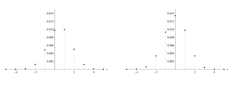
Figure 4: Plot of $g(r,s;12|0,0)$ with $q_{0,0}=q_{1,0}=1/2$, $q_{0,1}=q_{1,2}=1/3$ and $q_{0,2}=q_{1,1}=1/6$ for $r=1$ (on the left) and $r=2$ (on the right).

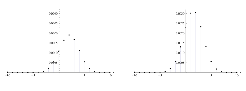
Figure 5: Plot of $g(r,s;30|0,0)$ with $q_{0,0}=q_{1,0}=1/2$, $q_{0,1}=q_{1,2}=1/3$ and $q_{0,2}=q_{1,1}=1/6$ for $r=1$ (on the left) and $r=2$ (on the right).

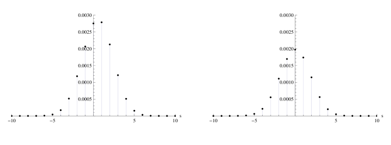
Figure 6: Plot of $g(r,s;30|0,0)$ with $q_{0,0}=q_{1,0}=1/2$, $q_{0,1}=q_{1,2}=1/3$ and $q_{0,2}=q_{1,1}=1/6$ for $r=4$ (on the left) and $r=5$ (on the right).

The results obtained in Theorems 5.1 and 5.3, which rely on the symmetry property given in point (i) of Corollary 3.5, can be extended to other forms of boundaries by exploiting the symmetries in points (ii) and (iii) of such corollary.

With reference to (32) let us now introduce the following cumulative distribution function, for $r,\tilde{j},\tilde{k}\in\mathbb{Z}$ and $\tau\in\mathbb{N}_{0}$,

$$H(r;2\tau+2|\tilde{j},\tilde{k})=\mathbb{P}_{0}\Big{[}T_{r}(\tilde{j},\tilde{k})\leq 2\tau+2\Big{]}=\sum_{n=0}^{\tau}h(r;2n+2|\tilde{j},\tilde{k}).$$ (39)

As example, we show some plots of function (39) in Figure 7, for different choices of $r$. Clearly, it shows that $H(r;2\tau+2|\tilde{j},\tilde{k})$ is decreasing when $r$ increases, and thus the boundary ${\cal B}_{r}$ runs far from the initial state.

Figure 7: Plot of $H(r;2\tau+2|0,0)$ with $q_{0,0}=q_{1,0}=1/2$, $q_{0,1}=q_{1,2}=1/3$ and $q_{0,2}=q_{1,1}=1/6$ for $r=2$, $3$, $4$ (from top to bottom).

In the chemistry literature wide interest is given to the self-avoiding random walks on lattices, i.e. walks subject to the condition that no lattice site may be visited more than once (see, for instance, Domb (1969)). Indeed, in polymer science self-avoiding random walks are used as a simple way to describe polymeric chains. Unfortunately, mathematical calculations concerning such walks are quite hard, since the sample paths do not intersect themselves. In this setting, in analogy with (30), let us denote by $T_{r}^{\rm sa}(\tilde{j},\tilde{k})$ the first-passage time through ${\cal B}_{r}$ when the random walk $(X_{n},Y_{n})$ does not visit the hexagonal lattice sites more than once. Hence, since the number of self-avoiding random walks is less than the regular one, it is obvious that

$$\mathbb{P}_{0}[T_{r}^{\rm sa}(\tilde{j},\tilde{k})\leq 2\tau+2]\geq H(r;2\tau+2|\tilde{j},\tilde{k})\qquad\hbox{for all $r,\tilde{j},\tilde{k}\in\mathbb{Z}$ and $\tau\in\mathbb{N}_{0}$.}$$

In other terms, we have $T_{r}^{\rm sa}(\tilde{j},\tilde{k})\leq_{\rm st}T_{r}(\tilde{j},\tilde{k})$, where $\leq_{\rm st}$ denotes the usual stochastic order (see, for instance, Shaked and Shanthikumar (2007)). Consequently, making use of Theorem 5.3 and Eqs. (33) and (39), under the assumptions of Theorem 5.1 we can obtain useful lower bounds to $\mathbb{P}_{0}[T_{r}^{\rm sa}(\tilde{j},\tilde{k})\leq 2\tau+2]$. Such information is useful to investigate the first-reaching-time of a preassigned length along the $x$-axis for two-dimensional polymeric chains that grow according to random rules as those of the random walk on hexagonal lattices.

For the cases treated in Figure 7, from (39) one has $H(2;122|0,0)=0.7185$, $H(3;122|0,0)=0.5887$, $H(4;122|0,0)=0.4709$, for instance. These values provide suitable lower bounds to the probability that a polymeric chain described by a self-avoiding random walk, starting at the origin of the hexagonal lattice and growing according to the probabilistic rules given in Figure 7, before 122 steps reaches a location situated along the line ${\cal B}_{2}$, ${\cal B}_{3}$, ${\cal B}_{4}$, respectively.

6 Concluding Remarks

Random walks on hexagonal lattices have a long history. The properties usually studied are concerning the transient and the recurrent behavior. In this paper, by exploiting the fact that the hexagonal lattice is a bipartite graph, we have developed a generating function-based approach to obtain closed-form expression for the state probabilities of the random walk. The asymptotic behavior of such stochastic process has also been treated in terms of large deviation and moderate deviation theory. Finally, since the state probabilities satisfy customary symmetry properties (see Corollary 3.5) we have been able to obtain suitable first-passage-time probabilities in a closed form.

Specifically, the results obtained in Section 5 can be applied to several contexts. Indeed, first-passage-time problems deserve interest in a variety of situations where the first reaching time of critical states has a relevant role. For instance, with reference to the models treated by Prasad and Borges (2006) and Pulliam et al. (1992), first-passage times of random walks on a hexagonal lattice can describe the exit times from assigned regions of animals searching for resources. Similarly, in the honeycomb Poisson-Voronoi access cellular network model, first-passage times are useful to model the reaching of areas with weak signal for mobile users. Another example arising in polymer science has been mentioned at the end of Section 5.

Possible future developments of the present investigation deal with developing asymptotic results for hitting probabilities through regions of different form, along the line mentioned in Remark 4.4.

References

- Abramowitz and Stegun (1994) Abramowitz M., Stegun I.A. (1994) Handbook of Mathematical Functions with Formulas, Graph, and Mathematical Tables. Reprint of the 1972 edition. Dover, New York.
- Akyildiz et al. (2000) Akyildiz I.F., Lin Y.B., Lai W.R., Chen R.J. (2000) A new random walk model for PCS networks. IEEE J. Selec. Areas Comm. 18, No. 7, 1254–1260.
- Asmussen and Glynn (2007) Asmussen S., Glynn P.W. (2007) Stochastic simulation: algorithms and analysis. Stochastic Modelling and Applied Probability, 57. Springer, New York.
- Baccelli and Blaszczyszyn (2009) Baccelli F., Blaszczyszyn B. (2009) Stochastic Geometry and Wireless Networks, Volume II - Applications, INRIA & Ecole Normale Superieure, Paris.
- Blanchet and Lam (2012) Blanchet J., Lam H. (2012) State-dependent importance sampling for rare-event simulation: An overview and recent advances. Surv. Oper. Res. Manag. Sci. 17, 38–59.
- Böhm and Hornik (2010) Böhm W., Hornik K. (2010) On two-periodic random walks with boundaries. Stoch. Models 26, No. 2, 165–194.
- Boutillier (2007) Boutillier C. (2007) Non-Colliding paths in the honeycomb dimer model and the Dyson process. J. Stat. Phys. 129, 1117–1135.
- Collamore (1998) Collamore J.F. (1998) First passage times of general sequences of random vectors: a large deviations approach. Stochastic Process. Appl. 78, 97–130.
- Collamore (2002) Collamore J.F. (2002) Importance sampling techniques for the multidimensional ruin problem for general Markov additive sequences of random vectors. Ann. Appl. Probab. 12, 382–421.
- Cotfas (2000) Cotfas N. (2000) Random walks on carbon nanotubes and quasicrystals. J. Phys. A: Math. Gen. 33, 2917–2927.
- de Forcrand et al. (1986) de Forcrand P., Koukiou F., Petritis D. (1986) Self-avoiding random walks on the hexagonal lattice. J. Stat. Phys. 45, Nos. 3/4, 459–470.
- Dembo and Zeitouni (1998) Dembo A., Zeitouni O. (1998) Large Deviations Techniques and Applications, Second Edition. Springer-Verlag, New York.
- Di Crescenzo et al. (2014) Di Crescenzo A., Macci C., Martinucci B. (2014) Asymptotic results for random walks in continuous time with alternating rates. J. Stat. Phys. 154, 1352–1364.
- Di Crescenzo and Martinucci (2008) Di Crescenzo A., Martinucci B. (2008) A first-passage-time problem for symmetric and similar two-dimensional birth-death processes. Stoch. Models 24, 451–469.
- Domb (1969) Domb C. (1969) Self avoiding walks on lattices. In: Stochastic Processes in Chemical Physics, (Shuler K.E., editor), Wiley, New York.
- Feng and Kurtz (2006) Feng J., Kurtz T.G. (2006) Large Deviations for Stochastic Processes. American Mathematical Society, New York.
- Guillotin-Plantard (2005) Guillotin-Plantard N. (2005) Gillis’s random walks on graphs. J. Appl. Prob. 42, 295–301.
- Haghpanah et al. (2013) Haghpanah B., Oftadeh R., Papadopoulos J., Vaziri A. (2013) Self-similar hierarchical honeycombs. Proc. R. Soc. A 469, 20130022, pp. 19.
- Katzenbeisser and Panny (2002) Katzenbeisser W., Panny W. (2002) The maximal height of simple random walks revisited. J. Statist. Plann. Infer. 101, no. 1-2, 149–161.
- Kennedy et al. (1988) Kennedy T., Lieb E.H., Tasaki H. (1988) A two-dimensional isotropic quantum antiferromagnet with unique disordered ground state. J. Stat. Phys. 53, Nos. 1/2, 383–415.
- Kotani and Sunada (2006) Kotani M., Sunada T. (2006) Large deviation and the tangent cone at infinity of a crystal lattice. Math. Z. 254, 837–870.
- Lawler and Limic (2010) Lawler G.F., Limic V. (2010) Random walk: a modern introduction. Cambridge Studies in Advanced Mathematics, 123. Cambridge University Press, Cambridge.
- Masuda et al. (2017) Masuda N., Porter M.A., Lambiotte R. (2017) Random walks and diffusion on networks. Physics Reports 716–717, 1–58. With correction in 745, 96 (2018).
- Miri and Stark (2003) Miri M., Stark H. (2003) Persistent random walk in a honeycomb structure: Light transport in foams. Phys. Rev. E 68, 031102.
- Montroll (1964) Montroll E.W. (1964) Random walks on lattices. Proc. Sympos. Appl. Math., Vol. XVI pp. 193–220 Amer. Math. Soc., Providence, R.I.
- Montroll and Weiss (1965) Montroll E.W., Weiss G.H. (1965) Random walks on lattices. II. J. Math. Phys. 6, 167–181.
- Panny and Prodinger (2016) Panny W., Prodinger H. (2016) A combinatorial study of two-periodic random walks. Stoch. Models 32, no. 1, 160–178.
- Prasad and Borges (2006) Prasad B.R.G., Borges R.M. (2006) Searching on patch networks using correlated random walks: space usage and optimal foraging predictions using Markov chain models. J. Theor. Biol. 240, 241–249.
- Pulliam et al. (1992) Pulliam H.R., Dunning J.B. Jr., Liu J. (1992) Population dynamics in complex landscapes: a case study. Ecol. Appl. 2, no. 2, 165–177.
- Rubin (1965) Rubin R.J. (1965) Random-walk model of chain-polymer adsorption at a surface. J. Chem. Phys. 43, 2392–2407.
- Schuyler et al. (2005) Schuyler A.D., Chirikjian G.S., Lu J.Q., Johnson H.T. (2005) Random-walk statistics in moment-based tight binding and applications in carbon nanotubes. Phys. Rev. E 71, 046701.
- Shaked and Shanthikumar (2007) Shaked M., Shanthikumar J.G. (2007) Stochastic Orders. Springer Series in Statistics. Springer, New York.
- Sokolov et al. (1993) Sokolov I.M., Vogel R., Alemany P.A., Blumen A. (1993) Continuous-time random walk of a rigid triangle. J. Phys. A Math. Gen. 28, 6645–6653.
- Zumofen and Blumen (1982) Zumofen G., Blumen A. (1982) Energy transfer as a random walk. II. Two-dimensional regular lattices. J. Chem. Phys. 76, 3713–3731.