Scalar self-force for highly eccentric equatorial orbits in Kerr spacetime

Abstract

If a small “particle” of mass $\mu M$ (with $\mu\ll 1$) orbits a black hole of mass $M$, the leading-order radiation-reaction effect is an $\mathcal{O}(\mu^{2})$ “self-force” acting on the particle, with a corresponding $\mathcal{O}(\mu)$ “self-acceleration” of the particle away from a geodesic. Such “extreme–mass-ratio inspiral” systems are likely to be important gravitational-wave sources for future space-based gravitational-wave detectors. Here we consider the “toy model” problem of computing the self-force for a scalar-field particle on a bound eccentric orbit in Kerr spacetime. We use the Barack-Golbourn-Vega-Detweiler effective-source regularization with a 4th order puncture field, followed by an $e^{im\phi}$ (“m-mode”) Fourier decomposition and a separate time-domain numerical evolution in $2{+}1$ dimensions for each $m$. We introduce a finite worldtube that surrounds the particle worldline and define our evolution equations in a piecewise manner so that the effective source is only used within the worldtube. Viewed as a spatial region, the worldtube moves to follow the particle’s orbital motion. We use slices of constant Boyer-Lindquist time in the region of the particle’s motion, deformed to be asymptotically hyperboloidal and compactified near the horizon and $\mathcal{J}^{+}$. Our numerical evolution uses Berger-Oliger mesh refinement with 4th order finite differencing in space and time. Our computational scheme allows computation for highly eccentric orbits and should be generalizable to orbital evolution in the future. Our present implementation is restricted to equatorial geodesic orbits, but this restriction is not fundamental. We present numerical results for a number of test cases with orbital eccentricities as high as $0.98$. In some cases we find large oscillations (“wiggles”) in the self-force on the outgoing leg of the orbit shortly after periastron passage; these appear to be caused by the passage of the orbit through the strong-field region close to the background Kerr black hole.

This paper is dedicated to the memory of our late friends and colleagues Thomas Radke and Steven Detweiler.

I Introduction

Consider a small (compact) body of mass $\mu M$ (with $0<\mu\ll 1$) moving freely in an asymptotically flat background spacetime (e.g., Kerr spacetime) of mass $M$. This system emits gravitational radiation, and there is a corresponding radiation-reaction influence on the small body’s motion. Self-consistently calculating this motion and the emitted gravitational radiation (and in general, the perturbed spacetime) is a long-standing research question in general relativity.

There is also an astrophysical motivation for this calculation: If a neutron star or stellar-mass black hole of mass ${\sim}\,1$–$100M_{\odot}$ orbits a massive black hole of mass ${\sim}\,10^{5}$–$10^{7}M_{\odot}$, the resulting “extreme–mass-ratio inspiral” (EMRI) system is expected to be a strong astrophysical gravitational-wave (GW) source detectable by the planned Laser Interferometer Space Array (LISA) space-based gravitational-wave detector. LISA is expected to observe many such systems, some of them at quite high signal/noise ratios (Gair et al. (2004); Barack and Cutler (2004); Amaro-Seoane et al. (2007); Gair (2009)). The data analysis for, and indeed the detection of, such systems will generally require matched-filtering the detector data stream against appropriate precomputed GW templates. The problem of computing such templates provides the astrophysical motivation for our calculation.

We are particularly concerned with the case where the small body’s orbit is highly relativistic, so post-Newtonian methods (see, for example, (Damour, 1987, section 6.10); Blanchet (2014); Futamase and Itoh (2007); Blanchet (2011); Schäfer (2011) and references therein) are not reliably accurate. Since the timescale for radiation reaction to shrink the orbit is very long ($\sim\mu^{-1}M$) while the required resolution near the small body is very high ($\sim\mu M$), a direct “numerical relativity” integration of the Einstein equations (see, for example, Pretorius (2007); Hannam et al. (2009); Hannam (2009); Hannam and Hawke (2011); Campanelli et al. (2010) and references therein) would be prohibitively expensive (and probably insufficiently accurate) for this problem.

Instead, we use black hole perturbation theory, treating the small body as an $\mathcal{O}(\mu)$ perturbation on the background spacetime. For this work we attempt to calculate leading-order radiation-reaction effects, i.e., $\mathcal{O}(\mu)$ field perturbations and $\mathcal{O}(\mu^{2})$ radiation-reaction “self-forces” acting on the small body. Because of the technical difficulty of controlling gauge effects in gravitational perturbations, in this work we use a scalar-field “toy model” system with the expectation that the techniques developed and discoveries made in the scalar case will carry over to the gravitational case.

The obvious way to model the small body is as a small black hole. While conceptually elegant, this approach is technically somewhat complicated Poisson et al. (2011). Instead, we model the small body as a point particle. Although one may be concerned about potential foundational issues with this approach, in practice it works well and, importantly, it agrees with rigorous derivations that do not rely on the use of point particles.

The $\mathcal{O}(\mu)$ “MiSaTaQuWa” equations of motion for a gravitational point particle in a (strong-field) curved spacetime were first derived by Mino, Sasaki, and Tanaka Mino et al. (1997) and Quinn and Wald Quinn and Wald (1997) (also see Detweiler’s analysis Detweiler (2001)) and have recently been rederived in a more rigorous manner by Gralla and Wald Gralla and Wald (2008). See Poisson et al. (2011); Detweiler (2005); Barack (2009, 2011); Burko (2011); Detweiler (2011); Poisson (2011); Wald (2011) for general reviews of gravitational radiation-reaction dynamics.

The particle’s motion may be modelled as either (i) non-geodesic motion in the background Schwarzschild/Kerr spacetime under the influence of a radiation-reaction “self-force”, or (ii) geodesic motion in a perturbed spacetime. These two perspectives (which are in some ways analogous to Eulerian versus Lagrangian formulations of fluid dynamics) are equivalent Sago et al. (2008); in this work we use the formulation (i). The MiSaTaQuWa equations then give the self-force in terms of (the gradient of) the metric perturbation due to the particle, which must be computed using black-hole perturbation theory.

The computation of the field perturbation due to a point particle is particularly difficult because the “perturbation” is formally infinite at the particle and thus must be regularized. There are several different, but equivalent, regularization schemes known for this problem, notably the “mode-sum” or “$\ell$-mode” scheme developed by Barack and Ori Barack and Ori (2000); Barack (2000); Barack et al. (2002); Barack and Ori (2002, 2003), Detweiler, Messaritaki, and Whiting Detweiler and Whiting (2003); Detweiler et al. (2003), and Haas and Poisson Haas and Poisson (2006); the Green-function approach Anderson and Wiseman (2005); Casals et al. (2009, 2013); Wardell et al. (2014); and the “effective-source” scheme of Barack and Golbourn Barack and Golbourn (2007) and Vega and Detweiler Vega and Detweiler (2008).

For a detailed presentation of the different regularization/computation schemes and their advantages and disadvantages, see Wardell (2015). In the present context we observe that for a Kerr background the traditional mode-sum scheme becomes less desirable because the mode equations don’t separate: all the (infinite set of) modes remain coupled. While the coupled modes can still be treated numerically (see, e.g., Warburton and Barack (2011)), here we adopt a different approach, the effective-source regularization scheme.

As discussed in detail in Sec. II.1, the effective-source scheme’s basic concept is to analytically compute a “puncture field” which approximates the particle’s Detweiler-Whiting singular field Detweiler and Whiting (2003), then numerically solve for the difference between the actual field perturbation and the puncture field. We have previously described many of the details of the computation of the puncture field Wardell et al. (2012a); in this work we focus on the application of this scheme to a particular class of self-force computations.

Depending on how the partial differential equations (PDEs) are solved, there are two broad classes of self-force computations: frequency-domain and time-domain. Frequency-domain computations involve a Fourier transform of the PDEs in time, reducing the numerical computation to the solution of a set of ordinary differential equations (ODEs) (see, for example, Detweiler et al. (2003)). The resulting computations are typically very efficient and accurate for circular or near-circular particle orbits, but degrade rapidly in efficiency with increasing eccentricity of the particle’s orbit, becoming impractical for highly eccentric orbits Glampedakis and Kennefick (2002); Barack and Lousto (2005). In contrast, time-domain computations involve a direct numerical time-integration of the PDEs and are generally less efficient and accurate than frequency-domain computations. However, time-domain computations can accommodate arbitrary particle orbits with only modest penalties in performance and accuracy Barton et al. (2008), with some complications in the numerical schemes (see, for example, Haas (2007); Barack and Sago (2010)).

In this work our goal is to consider highly eccentric orbits,, so we follow the time-domain approach. We use standard Berger-Oliger mesh refinement techniques and compactified hyperboloidal slices for improved accuracy and efficiency.

The remainder of this paper is organized as follows:

Section I.1 summarizes our notation.

Section II gives a detailed description of our theoretical and computational formalism for self-force computations, with subsections on the effective source regularization (II.1), the $m$-mode Fourier decomposition (II.2), the worldtube (II.3), moving the worldtube (II.4), hyperboloidal slices and compactification (II.5), our reduction to a 1st-order-in-time system of evolution equations (II.6), the computation of the puncture field and effective source (II.7), the computation of the effective source close to the particle (II.8), boundary conditions (II.9), initial data (II.10), how the self-force is computed from our evolved field variables (II.11), the large-$m$ “tail series” (II.12), selecting the time interval for analysis within an evolution (II.13), selecting a “low-noise” subset of times within an evolution (II.14), how we split the self-force into dissipative and conservative parts (II.15), and a summary of our computation and data analysis (II.16).

Section III presents our numerical results and compares them to values obtained by other authors, with subsections on our test configurations and parameters (III.1), an example of our data analysis (III.2), the convergence of our results with numerical resolution (III.3), a numerical verification that our results are independent of the choice of worldtube and other numerical parameters (III.4), comparison of our results with those of other researchers (III.5), an overview of our computed self-force for each configuration (III.6), our results for highly eccentric orbits (III.7), our results for zoom-whirl orbits (III.8), and strong oscillations (“wiggles”) in the self-force shortly after periastron (III.9).

Section IV presents a general discussion of this work, the conclusions to be drawn from it, and some directions for future research.

Appendix A describes the transformation between $\tilde{\phi}$ and $\phi$ derivatives, where $\tilde{\phi}$ is the “untwisted” azimuthal coordinate defined by (10).

Appendix B describes our computational scheme in more detail, with subsections on the numerical computation of $r(r_{*})$ (B.1), the numerical integration of equatorial eccentric Kerr geodesics (B.2), gradual turnon of the effective source (B.3), our algorithm for moving the worldtube (B.4), constraints on moving the worldtube early in the time evolution (B.5), finite differencing across the worldtube boundary (B.6), computing the set of grid points where adjusted finite differencing is needed (B.7), computing the set of grid points where the puncture field is needed (B.8), the numerical time-evolution using Berger-Oliger mesh refinement (B.9), finite differencing near the particle (B.10), and implicit-explicit (IMEX) evolution schemes (B.11).

I.1 Notation

We generally follow the sign and notation conventions of Wald Wald (1984), with $G=c=1$ units and a $(-,+,+,+)$ metric signature. We use the Penrose abstract-index notation, with indices $abcd$ running over spacetime coordinates, $ijk$ running over the spatial coordinates, $\ell$ running over only the $m$-mode coordinates $(t,r,\theta)$, and $s$ running over only the spatial $m$-mode coordinates $(r,\theta)$ (in both of the latter cases, the coordinates are defined by (1) below). $\nabla_{a}$ is the (spacetime) covariant derivative operator. $X:=Y$ means that $X$ is defined to be $Y$. $\Box:=\nabla_{a}\nabla^{a}$ is the 4-dimensional (scalar) wave operator Brill et al. (1972); Teukolsky (1973). $\mathop{\text{conj}}\left[z\right]$ is the complex conjugate of the complex number $z$. ${\partial S}$ is the boundary of the set $S$. $(a)_{n}$ denotes the Pochhammer symbol $\displaystyle\Pi_{k=a}^{a+n-1}k$.

We use Boyer-Lindquist coordinates $(t,r,\theta,\phi)$ on Kerr spacetime, defined by the line element

$$ds^{2}={} -\left(1-\frac{2Mr}{\Sigma}\right)\,dt^{2}-4M^{2}\tilde{a}\frac{r\sin^{2}\theta}{\Sigma}\,dt\,d\phi$$

$$+\frac{\Sigma}{\Delta}\,dr^{2}+\Sigma\,d\theta^{2}$$

$$+\left(r^{2}+M^{2}\tilde{a}^{2}+2M^{3}\tilde{a}^{2}\frac{r\sin^{2}\theta}{\Sigma}\right)\sin^{2}\theta\,d\phi^{2},$$ (1)

where $M$ is the spacetime mass, $\tilde{a}=J/M^{2}$ is the dimensionless spin of the black hole (limited to $|\tilde{a}|<1$), $\Sigma=r^{2}+M^{2}\tilde{a}^{2}\cos^{2}\theta$, and $\Delta=r^{2}-2Mr+M^{2}\tilde{a}^{2}$. In Boyer-Lindquist coordinates the event horizon is the coordinate sphere $r=r_{h}=r_{+}=M\left(1+\sqrt{1-\tilde{a}^{2}}\right)$ and the inner horizon is the coordinate sphere $r=r_{-}=M\left(1-\sqrt{1-\tilde{a}^{2}}\right)$.

We take the particle to orbit in the equatorial plane in the $d\phi/dt>0$ direction, with $\tilde{a}>0$ for prograde orbits and $\tilde{a}<0$ for retrograde orbits. We parameterize the particle’s (bound equatorial geodesic) orbit by the usual dimensionless semi-latus rectum $p$ and eccentricity $e$; these are defined in detail in Appendix B.2. We refer to the combination of a spacetime and a particle orbit as a “configuration”, and parameterize it with the triplet $(\tilde{a},p,e)$. We define $T_{r}$ to be the coordinate-time period of the particle’s radial motion; we usually refer to $T_{r}$ as the particle’s “orbital period”. We define the “modulo time” to be the coordinate time modulo $T_{r}$.

To aid in assessing the accuracy of our computed self-forces, we define a positive-definite pointwise norm on covariant or contravariant 4-vectors,

$$\|v_{a}\|_{+} :=\left(|v_{t}v^{t}|+|v_{i}v^{i}|\right)^{1/2}$$ (2a)

$$\|v^{a}\|_{+} :=\left(|v_{t}v^{t}|+|v_{i}v^{i}|\right)^{1/2},$$ (2b)

where all indices are raised and lowered with the Boyer-Lindquist 4-metric.

We use $x^{a}_{\text{particle}}(t)$ to denote the particle’s worldline, which we consider to be known in advance, i.e., we do not consider changes to the particle’s worldline induced by the self-force. $\mathcal{E}$ and $\mathcal{L}$ are the particle’s specific energy and specific angular momentum (i.e., the particle’s energy and angular momentum per unit mass).

When referring to finite difference molecules (stencils) we use i and j as generic integer grid coordinates in the radial ($R_{*}$) and angular ($\theta$) directions, respectively (where $R_{*}$ is the compactified tortise coordinate defined by (18), (29), and (30)). Considering a finite difference molecule evaluated at the grid point $(\texttt{i},\texttt{j})$, we define the molecule’s “radius” in a given direction ($\texttt{i}+$, $\texttt{i}-$, $\texttt{j}+$, or $\texttt{j}-$) as the maximum integer $\delta\geq 0$ such that the molecule has a nonzero coefficient at $\texttt{i}\pm\delta$ or $\texttt{j}\pm\delta$, respectively, and we refer to these as $R_{\texttt{i}+}$, $R_{\texttt{i}-}$, $R_{\texttt{j}+}$, and $R_{\texttt{j}-}$ respectively. For example, the usual 3-point centered 2nd-order molecule approximating the radial partial derivative $\partial_{R_{*}}$ has $R_{\texttt{i}+}=R_{\texttt{i}-}=1$ and $R_{\texttt{j}+}=R_{\texttt{j}-}=0$.

We use a pseudocode notation to describe algorithms: Lines are numbered for reference, but the line numbers are not used in the algorithm itself. # marks comment lines, while keywords are typeset in bold font. Procedures are marked with the keyword procedure and have bodies delimited by “$\{$” and “$\}$”. Code layout and indentation are solely for clarity and (unlike Python) do not have any explicit semantics. Procedure names are typeset in typewriter font. Value-returning procedures (functions) have an explicitly-declared return type (e.g., “boolean procedure”) and return a value with a return statement. When referring to a procedure as a noun in a figure caption or in the main text of this paper, the procedure name is suffixed with “()”, as in “foo()”.

Variable names are either mathematical expressions, such as “$R_{i+}$”, or are typeset in typewriter font. “$\texttt{var}\leftarrow X$” means that the variable var is assigned the value of the expression $X$. Variables are always declared before use. The declaration of a variable explicitly states the variable’s type (integer, floating_point, interval, or region, the last of these being a rectangular region in the integer plane $\mathbb{Z}\,{\times}\,\mathbb{Z}$) and may also be combined with the assignment of an initial value, as in “region $W\leftarrow\text{worldtube region}$”. Conditional expressions have C-style syntax and semantics, condition ? expression-if-true : expression-if-false, while conditional statements have explicit if, then, and else keywords.

In Appendix B.11 we use lower-case sans-serif letters $\mathsf{u}$, $\mathsf{k}$, and $\tilde{\mathsf{k}}$ for state vectors, and upper-case sans-serif letters $\mathsf{F}$ and $\mathsf{G}$ for state-vector-valued functions.

II Theoretical formalism

Ignoring questions of divergence and regularization near the particle, in general the (4-vector) radiation-reaction self-force on a scalar particle moving in an arbitrary (specified) background spacetime is given by

$$F_{a}=q\,\bigl{.}(\nabla_{a}\Phi)\bigr{|}_{\text{particle}},$$ (3)

where the particle’s scalar charge is $q$ (which may vary along the particle’s worldline), and the (real) scalar field $\Phi$ satisfies the wave equation

$$\Box\Phi=q\,\delta\bigl{(}x^{a}-x^{a}_{\text{particle}}(t)\bigr{)},$$ (4)

where $\Box$ is the curved-space wave operator in the background spacetime Brill et al. (1972).

Because of the $\delta$-function source in (4), $\Phi$ diverges on the particle’s worldline, so that some type of regularization is essential in order to obtain a finite self-force.

II.1 Effective source regularization

We use the “effective-source” or “puncture-field” regularization scheme introduced by Barack and Golbourn Barack and Golbourn (2007) and Vega and Detweiler Vega and Detweiler (2008) (see Vega et al. (2011) for a recent review). This regularization is based on the Detweiler-Whiting decomposition Detweiler and Whiting (2003) of $\Phi$ into the sum of a “singular” and a “regular” field, $\Phi=\Phi_{\text{singular}}+\Phi_{\text{regular}}$, with the following properties:

• The singular field is divergent on the particle’s worldline but is (in a suitable sense) spherically symmetric at the particle and hence exerts no self-force.

• The regular field is finite – in fact $C^{\infty}$ – at the particle and exerts the entire self-force. That is, the correct self-force may be obtained by applying (3) to the regular field,

  $$F_{a}=q\,\bigl{.}(\nabla_{a}\Phi_{\text{regular}})\bigr{|}_{\text{particle}}.$$ (5)

Unfortunately, it is very difficult to compute the exact Detweiler-Whiting singular or regular fields in Schwarzschild or Kerr spacetime. The basic concept of the effective-source regularization is to instead compute a “puncture field” approximation $\Phi_{\text{puncture}}\approx\Phi_{\text{singular}}$, chosen (in a manner to be described in detail below) so that the “residual field” $\Phi_{\text{residual}}:=\Phi-\Phi_{\text{puncture}}$ is finite and “somewhat differentiable” (in our case $C^{2}$) in a neighborhood of the particle. We then have

$$\Box\Phi_{\text{residual}} =\Box\Phi-\Box\Phi_{\text{puncture}}$$

$$=q\,\delta\bigl{(}x-x_{\text{particle}}(t)\bigr{)}-\Box\Phi_{\text{puncture}}$$

$$=\begin{cases}0&\begin{tabular}[t]{@{}l@{}}on the particle worldline\\[-2.15277pt] (our choice of $\Phi_{\text{puncture}}$ will ensure this)\end{tabular}\\ -\Box\Phi_{\text{puncture}}&\text{elsewhere}\end{cases}$$ (6)

$$:=S_{\text{effective}},$$ (7)

where we define the “effective source” $S_{\text{effective}}$ to be the right hand side of (6).

In more detail, we choose $\Phi_{\text{puncture}}$ so that for some chosen integer $n\geq 3$,

$$\Phi_{\text{puncture}}-\Phi_{\text{singular}}=\mathcal{O}\bigl{(}\|x\,{-}\,x_{\text{particle}}(t)\|^{n-1}\bigr{)}$$ (8)

in a neighborhood of the particle. (This is equivalent to choosing $\Phi_{\text{puncture}}$ so that its Laurent series about the particle position matches the first $n$ terms of $\Phi_{\text{singular}}$’s Laurent series; both series begin with $\bigl{\|}x\,{-}\,x_{\text{particle}}(t)\bigr{\|}^{-1}$ terms.) Since $\Phi_{\text{regular}}$ is $C^{\infty}$ at the particle and $\Phi_{\text{residual}}=\Phi_{\text{regular}}+(\Phi_{\text{singular}}-\Phi_{\text{puncture}})=\Phi_{\text{regular}}+\mathcal{O}\bigl{(}\|x\,{-}\,x_{\text{particle}}(t)\|^{n-1}\bigr{)}$ in a neighborhood of the particle, we have $\bigl{.}(\nabla\Phi_{\text{residual}})\bigr{|}_{\text{particle}}=\bigl{.}(\nabla\Phi_{\text{regular}})\bigr{|}_{\text{particle}}$. By virtue of (5) the radiation-reaction self-force is thus given by

$$F_{a}=q\,\bigl{.}(\nabla_{a}\Phi_{\text{residual}})\bigr{|}_{\text{particle}}.$$ (9)

In this work we choose $n=4$, so that $\Phi_{\text{residual}}$ is $C^{2}$ at the particle and $S_{\text{effective}}$ is $C^{0}$ at the particle. Note, however, that the criterion (8) still leaves considerable freedom in the choice (definition) of $\Phi_{\text{puncture}}$. We describe our choice in detail in section II.7.

II.2 $m$-mode Fourier decomposition

Given the basic effective-source formalism, some authors (e.g., Vega and Detweiler (2008); Vega et al. (2009, 2011); Diener et al. (2012); Vega et al. (2013)) choose to solve (7) via a direct numerical integration in $3{+}1$ dimensions. However, following Barack and Golbourn (2007); Barack et al. (2007); Dolan and Barack (2011); Dolan et al. (2011); Dolan and Barack (2013), we prefer instead to exploit the axisymmetry of the background (Kerr) spacetime and introduce an $m$-mode (Fourier) decomposition.

To avoid infinite twisting of the Boyer-Lindquist $\phi$ coordinate at the event horizon, we follow Krivan et al. (1996) by introducing an “untwisted” azimuthal coordinate

$$\tilde{\phi}=\phi+f(r)$$ (10)

with the function $f$ chosen such that

$$d\tilde{\phi}=d\phi+\frac{M\tilde{a}}{\Delta}dr.$$ (11)

It is straightforward to integrate this to give

$$f(r)=\frac{\tilde{a}}{2\sqrt{1-\tilde{a}^{2}}}\ln\left|\frac{r-r_{+}}{r-r_{-}}\right|+\text{constant}.$$ (12)

Using the $\tilde{\phi}$-derivative transformations derived in Appendix A, $\Box\Phi$ can be written in $(t,r,\theta,\tilde{\phi})$ coordinates as

$$\Sigma\Box\Phi={} -\left[\frac{(r^{2}+M^{2}\tilde{a}^{2})^{2}}{\Delta}-M^{2}\tilde{a}^{2}\sin^{2}\theta\right]\partial_{tt}\Phi$$

$$-\frac{4M^{2}\tilde{a}r}{\Delta}\partial_{t\tilde{\phi}}\Phi+\partial_{r}\Bigl{(}\Delta\partial_{r}\Phi\Bigr{)}+2M\tilde{a}\partial_{r\tilde{\phi}}\Phi$$

$$+\partial_{\theta\theta}\Phi+\cot\theta\,\partial_{\theta}\Phi+\frac{1}{\sin^{2}\theta}\partial_{\tilde{\phi}\tilde{\phi}}\Phi.$$ (13)

We Fourier-decompose the field in $e^{im\tilde{\phi}}$ modes, writing

$$\Phi(t,r,\theta,\phi)=\sum_{m=-\infty}^{\infty}e^{im\tilde{\phi}}\Psi_{m}(t,r,\theta)$$ (14)

and analogously for the other fields $\Phi_{\text{puncture}}$, $\Phi_{\text{residual}}$, and $S_{\text{effective}}$. For each integer $m$, the (complex) $m$-mode fields are given by

$$\Psi_{m}(t,r,\theta)=\frac{1}{2\pi}\int_{-\pi}^{\pi}\Phi(t,r,\theta,\phi)e^{-im\tilde{\phi}}\,d\tilde{\phi}$$ (15)

and analogously for the other fields $\Psi_{\text{puncture},m}$, $\Psi_{\text{residual},m}$, and $S_{\text{effective},m}$. We then introduce the (complex) radial-factored field

$$\varphi_{m}=r\Psi_{m}$$ (16)

(and analogously for $\varphi_{\text{puncture},m}$ and $\varphi_{\text{residual},m}$) so that the far-field falloffs around an asymptotically-flat system are $\varphi_{m}=\mathcal{O}(1)$ when $\Psi_{m}=\mathcal{O}(1/r)$.

Following Sundararajan et al. (2007), we introduce the tortise coordinate $r_{*}$ defined (up to an arbitrary additive constant) by

$$\frac{dr_{*}}{dr}=\frac{r^{2}+M^{2}\tilde{a}^{2}}{\Delta}.$$ (17)

Again following Sundararajan et al. (2007), we fix the additive constant by choosing

$$r_{*}={} r+2M\frac{r_{+}}{r_{+}-r_{-}}\ln\left(\frac{r-r_{+}}{2M}\right)$$

$$\phantom{r}-2M\frac{r_{-}}{r_{+}-r_{-}}\ln\left(\frac{r-r_{-}}{2M}\right).$$ (18)

We describe the numerical computation of $r(r_{*})$ in Appendix B.1. For any scalar quantity $Q$ we have (using the chain rule)

$$\frac{\partial Q}{\partial r}=\frac{r^{2}+M^{2}\tilde{a}^{2}}{\Delta}\frac{\partial Q}{\partial r_{*}}.$$ (19)

The scalar wave operator $\Box\Phi$ then becomes

$$\Box\Phi=\sum_{m=-\infty}^{\infty}\frac{e^{im\tilde{\phi}}}{r}\,\Box_{m}\varphi_{m}$$ (20)

and each $m$-mode of the residual field satisfies

$$\Box_{m}\varphi_{\text{residual},m}=S_{\text{effective},m}\,,$$ (21)

where

$$\Box_{m}\varphi_{=}{} -\frac{1}{r\Sigma}\left[\frac{(r^{2}+M^{2}\tilde{a}^{2})^{2}}{\Delta}-M^{2}\tilde{a}^{2}\sin^{2}\theta\right]\partial_{tt}\varphi-4im\frac{M^{2}\tilde{a}}{\Delta\Sigma}\partial_{t}\varphi$$

$$+\frac{(r^{2}+M^{2}\tilde{a}^{2})^{2}}{r\Delta\Sigma}\partial_{r_{*}r_{*}}\varphi+\left[-2\frac{M^{2}\tilde{a}^{2}}{r^{2}\Sigma}+2imM\tilde{a}\frac{r^{2}+M^{2}\tilde{a}^{2}}{r\Delta\Sigma}\right]\partial_{r_{*}}\varphi$$

$$+\frac{1}{r\Sigma}\partial_{\theta\theta}\varphi+\frac{\cot\theta}{r\Sigma}\partial_{\theta}\varphi-\left[\frac{2}{r^{2}\Sigma}\left(M-\frac{M^{2}\tilde{a}^{2}}{r}\right)+\frac{m^{2}}{r\Sigma\sin^{2}\theta}+2im\frac{M\tilde{a}}{r^{2}\Sigma}\right]\varphi.$$ (22)

II.3 The worldtube

Our construction of the puncture field and effective source (Wardell et al. (2012a) and Sec. II.7) is only valid in an finite $(r,\theta)$ neighborhood of the particle. Moreover, it is not clear what far-field boundary conditions the residual field should satisfy. Therefore, rather than solving (21) directly, for each $m$ we introduce a finite worldtube $W_{m}$ chosen so that its interior contains the particle worldline, and the puncture field and effective source are defined everywhere in the worldtube. (Notice that $W_{m}$ logically “lives” in the $m$-mode $(t,r,\theta)$ space, not in spacetime.)

For each $m$ we define the piecewise “numerical field”

$$\varphi_{\text{num},m}=\begin{cases}\varphi_{\text{residual},m}&\text{in the worldtube}\\ \varphi_{m}&\text{outside the worldtube}\end{cases}.$$ (23)

This field has a jump discontinuity across the worldtube boundary,

$$\lim_{\begin{subarray}{c}x^{\ell}\to b^{\ell}\\ x^{\ell}\in W_{m}\end{subarray}}\!\!\varphi_{\text{num},m}(x^{\ell})=\biggl{[}\lim_{\begin{subarray}{c}x^{\ell}\to b^{\ell}\\ x^{\ell}\not\in W_{m}\end{subarray}}\!\!\varphi_{\text{num},m}(x^{\ell})\biggr{]}-\varphi_{\text{puncture},m}(b^{\ell})$$ (24)

for any worldtube-boundary point $b^{\ell}\in{\partial W_{m}}$, and it also satisfies

$$\Box_{m}\varphi_{\text{num},m}=\begin{cases}S_{\text{effective},m}&\text{inside the worldtube}\\ 0&\text{outside the worldtube}.\end{cases}$$ (25)

We numerically solve (25) via a separate Cauchy time-evolution for each $m$. The form of (25) ensures that the effective source only needs to be computed inside the worldtube, and (as discussed in detail in Sec. II.4 and Appendices B.6 and B.8) the puncture field only needs to be computed within a small neighborhood of the worldtube boundary.

The precise choice of the worldtube may be made for computational convenience; by construction, the computed self-force is independent of this choice (see Sec. III.4 for a numerical verification of this independence). The worldtube’s size should reflect a tradeoff between numerical cost and accuracy:

• A larger worldtube requires computing $S_{\text{effective},m}$ (which is expensive) at a larger set of events.

• A smaller worldtube (more precisely, one whose complement includes points closer to the particle) requires numerically computing – and hence finite differencing – $\varphi_{m}$ closer to its singularity at the particle, leading to larger numerical errors.

For a given worldtube shape and size, the best accuracy is generally obtained by choosing the worldtube to be approximately centered on the particle.

In practice we typically choose a worldtube which is a rectangle in $(r_{*},\theta)$ of half-width $5\,M$ in $r_{*}$ and approximately $\pi/8$ in $\theta$.

Since we use Berger-Oliger mesh refinement (Appendix B.9), the question arises of how the worldtube should interact with the mesh refinement. In particular, should the worldtube differ from one refinement level to another? For simplicity we have chosen a computational scheme where this is not the case – in our scheme the worldtube is the same at all refinement levels. This means that the Berger-Oliger mesh-refinement algorithm does not need to make the adjustment (26) when copying or interpolating data between different refinement levels. The worldtube boundary is effectively quantized to the coarsest (base) grid, but we do not find this to be a problem in practice.

II.4 Moving the worldtube

If the particle’s orbit has a sufficiently small eccentricity then a reasonably-sized time-independent worldtube in $(r_{*},\theta)$ can encompass the particle’s entire orbital motion. However, our main interest is in the case where the particle’s orbit is highly eccentric. This requires the worldtube to be time-dependent in order to enclose the particle throughout the particle’s entire orbital motion. In our computational scheme we move the worldtube in $(r_{*},\theta)$ in discontinuous jumps so as to always keep the worldtube’s coordinate center within a small distance (typically $\sim 0.5\,M$) of the particle position. (More precisely, this is the case after the startup phase of the computation; we discuss this in detail in Sec. B.5.)

When the worldtube moves, those “transition” grid points which were formerly inside the worldtube and are now outside, or vice versa, essentially have the computation of $\Box\varphi_{\text{puncture}}$ switched between being done analytically versus via finite differencing. In the continuum limit these two computations agree, but at finite resolutions they differ slightly. Therefore, moving the worldtube introduces numerical noise into the evolved field $\varphi_{\text{num},m}$.

Our actual worldtube-moving algorithm (described in detail in Appendix B.4) incorporates a number of refinements to help mitigate this numerical noise and achieve the most accurate numerical evolutions possible:

• Basically, the algorithm moves the worldtube any time the particle position is “too far” from the worldtube center.

• When moving the worldtube, the algorithm places the new worldtube center somewhat ahead of the particle in the direction of the particle’s motion. The algorithm includes a small amount of hysteresis so as to avoid unnecessary back-and-forth worldtube moves.

• The algorithm limits the maximum distance the worldtube can be moved at any one time.

• The algorithm imposes a minimum time interval between worldtube moves.

Because $\varphi_{\text{num},m}$ has the jump discontinuity (24) across the worldtube boundary, each time the worldtube is moved the evolved fields $\varphi_{\text{num},m}$ and $\Pi_{\text{num},m}$ must be adjusted at transition grid points:

$$\varphi_{\text{num},m} \leftarrow\varphi_{\text{num},m}\pm\varphi_{\text{puncture},m}$$ (26a)

$$\Pi_{\text{num},m} \leftarrow\Pi_{\text{num},m}\pm\partial_{t}\varphi_{\text{puncture},m}\,,$$ (26b)

where the “$+$” applies to grid points which were formerly inside the worldtube and are now outside it, and the “$-$” applies to grid points which were formerly outside the worldtube and are now inside it.

II.5 Hyperboloidal slices and compactification

Conceptually, (25) should be solved on the entire spacetime, with outflow boundary conditions on the event horizon and null infinity ($\mathcal{J}^{+}$). To accomplish this computationally, we use a hyperboloidal compactification scheme developed by Zenginoğlu Zenginoğlu (2008a, b, 2011); Zenginoğlu and Khanna (2011); Zenginoğlu and Kidder (2010); Zenginoğlu and Tiglio (2009); Bernuzzi et al. (2011, 2012). This scheme has a number of desirable properties, including:

1. The hyperboloidal slices reach the event horizon and $\mathcal{J}^{+}$, allowing pure-outflow boundary conditions to be posed there.

2. The transformed evolution equations do not suffer the “infinite blue-shifting” problem (cf. the discussion of Zenginoğlu (2011)) in the compactification region – they have finite and nonzero propagation speeds throughout the computational domain, and outgoing waves suffer at most $\mathcal{O}(1)$ compression (blue-shifting) or expansion (red-shifting) as they propagate from the region of the particle to the event horizon and to ${\mathcal{J}^{+}}$.

3. The transformed evolution equations can be formulated to be nonsingular everywhere, with all coefficients having finite limiting values near to and on both the event horizon and $\mathcal{J}^{+}$.

4. The (time-independent) compactification transformation can be chosen to be the identity transformation throughout a neighborhood of the entire range of the particle’s orbital motion. This means that the computation of the effective source and puncture field, the various adjustments to the computations when crossing the worldtube boundary or when moving the worldtube, and the computation of the self-force from the evolved field $\varphi_{m}$, are all unaffected by the compactification.

5. The scheme is easy to implement, requiring only relatively modest modifications to our previous (non-compactified) numerical code.

We primarily follow the version of Zenginoğlu’s compactification scheme described in Zenginoğlu and Khanna (2011), although with slightly different notation to more conveniently allow a unified treatment of compactification near the event horizon and near $\mathcal{J}^{+}$.

For purposes of compactification, it is convenient to rewrite the evolution equation (25) and (22) in the generic form

$$C[\partial_{tt}\varphi]\partial_{tt}\varphi+C[\partial_{tr_{*}}\varphi]\partial_{tr_{*}}\varphi+C[\partial_{r_{*}r_{*}}\varphi]\partial_{r_{*}r_{*}}\varphi$$

$$+C[\partial_{t}\varphi]\partial_{t}\varphi+C[\partial_{r_{*}}\varphi]\partial_{r_{*}}\varphi$$

$$+C[\partial_{\theta\theta}\varphi]\partial_{\theta\theta}\varphi+C[\partial_{\theta}\varphi]\partial_{\theta}\varphi$$

$$+C[\varphi]\varphi+C[1] =0,$$ (27)

where we have dropped the subscript on $\varphi_{m}$, and where the $C[\cdot]$ coefficients can be read off from the evolution equations. ($C[\partial_{tr_{*}}\varphi]=0$ for our evolution equations, but is included for generality.)

To make the equations nonsingular near to and on the event horizon, we multiply (25) through by a factor of $r\Sigma\Delta$. It is also useful for the coefficients to be finite near to and at $\mathcal{J}^{+}$, so we further multiply through by a factor of $(r^{2}+M^{2}\tilde{a}^{2})^{-2}$. The resulting coefficients are

$$C[\partial_{tt}\varphi] =\frac{M^{2}\tilde{a}^{2}\Delta\sin^{2}\theta}{(r^{2}+M^{2}\tilde{a}^{2})^{2}}-1,$$ (28a)

$$C[\partial_{t}\varphi] =-i\frac{4mM^{2}\tilde{a}r}{(r^{2}+M^{2}\tilde{a}^{2})^{2}},$$ (28b)

$$C[\partial_{r_{*}r_{*}}\varphi] =1,$$ (28c)

$$C[\partial_{r_{*}}\varphi] =-\frac{2M^{2}\tilde{a}^{2}\Delta}{r(r^{2}+M^{2}\tilde{a}^{2})^{2}}+i\frac{2mM\tilde{a}}{r^{2}+M^{2}\tilde{a}^{2}},$$ (28d)

$$C[\partial_{\theta\theta}\varphi] =\frac{\Delta}{(r^{2}+M^{2}\tilde{a}^{2})^{2}},$$ (28e)

$$C[\partial_{\theta}\varphi] =\frac{\Delta\cot\theta}{(r^{2}+M^{2}\tilde{a}^{2})^{2}},$$ (28f)

$$C[\varphi] =-\frac{2\Delta}{r(r^{2}+M^{2}\tilde{a}^{2})^{2}}\left(M-\frac{M^{2}\tilde{a}^{2}}{r}\right)$$

$$\quad-\frac{m^{2}\Delta}{(r^{2}+M^{2}\tilde{a}^{2})^{2}\sin^{2}\theta}-i\frac{2mM\tilde{a}\Delta}{r(r^{2}+M^{2}\tilde{a}^{2})^{2}},$$ (28g)

$$C[1] =\begin{cases}\begin{aligned} &-\dfrac{r\Sigma\Delta}{(r^{2}+M^{2}\tilde{a}^{2})^{2}}S_{\text{effective},m}&&\text{inside}\\ &0&&\text{outside}.\end{aligned}\end{cases}$$ (28h)

We define the compactified radial coordinate $R_{*}$ by

$$r_{*}=\frac{R_{*}}{\Omega(R_{*})},$$ (29)

where we choose the (time-independent) conformal factor $\Omega$ so that the event horizon and $\mathcal{J}^{+}$ are at the (finite) $R_{*}$ coordinates $R_{*}^{h}$ and $R_{*}^{\mathcal{J}^{+}}$ respectively. More precisely, we introduce the four parameters $R_{*}^{h}<R_{*}^{-}<0<R_{*}^{+}<R_{*}^{\mathcal{J}^{+}}$, chosen such that the particle and worldtube always lie within the region $R_{*}^{-}<R_{*}<R_{*}^{+}$ (where we will choose the compactification transformation to be the identity transformation). We define

$$\Omega(R_{*})=\begin{cases}\displaystyle 1-\left(\frac{R_{*}^{-}-R_{*}}{R_{*}^{-}-R_{*}^{h}}\right)^{4}&\text{if $R_{*}<R_{*}^{-}$}\\ 1&\text{if $R_{*}^{-}\leq R_{*}\leq R_{*}^{+}$}\\ \displaystyle 1-\left(\frac{R_{*}-R_{*}^{+}}{R_{*}^{\mathcal{J}^{+}}-R_{*}^{+}}\right)^{4}&\text{if $R_{*}>R_{*}^{+}$}\end{cases}$$ (30)

so that the compactification transformation is indeed the identity transformation ($\Omega=1$ and $r_{*}=R_{*}$) throughout the region $R_{*}^{-}<R_{*}<R_{*}^{+}$. We refer to $R_{*}^{-}$ and $R_{*}^{+}$ as the inner and outer compactification radii, respectively. Our numerical grid spans the full range $R_{*}^{h}\leq R_{*}\leq R_{*}^{\mathcal{J}^{+}}$.

To ensure the absence of infinite blue-shifting (“desirable property” 2), the time coordinate must also be transformed. We define the transformed time coordinate $T$ by

$$T=t-h(R_{*}),$$ (31)

where the “height” function $h$ is given by

$$h(R_{*}) =\begin{cases}R_{*}-r_{*}&\text{if $R_{*}<R_{*}^{-}$}\\ 0&\text{if $R_{*}^{-}\leq R_{*}\leq R_{*}^{+}$}\\ r_{*}-R_{*}&\text{if $R_{*}>R_{*}^{+}$}\end{cases}$$

$$=\begin{cases}\displaystyle R_{*}\left(1-\frac{1}{\Omega}\right)&\text{if $R_{*}<R_{*}^{-}$}\\ 0&\text{if $R_{*}^{-}\leq R_{*}\leq R_{*}^{+}$}\\ \displaystyle R_{*}\left(\frac{1}{\Omega}-1\right)&\text{if $R_{*}>R_{*}^{+}$}\end{cases}.$$ (32)

In order to express the equations in a simple form, it is convenient to define the “generalized boost” function

$${\,\overline{\!{\vrule height=7.74998pt,depth=0.0pt,width=0.0pt}H\!}\,}=\frac{dR_{*}}{dr_{*}}=\frac{\Omega^{2}}{\Omega-R_{*}\Omega^{\prime}},$$ (33)

where $X^{\prime}:=dX/dR_{*}$ for any quantity $X$, so that

$${\,\overline{\!{\vrule height=7.74998pt,depth=0.0pt,width=0.0pt}H\!}\,}^{\prime}=\frac{2\Omega\Omega^{\prime}}{\Omega-R_{*}\Omega^{\prime}}+\frac{R_{*}\Omega^{2}\Omega^{\prime\prime}}{(\Omega-R_{*}\Omega^{\prime})^{2}}$$ (34)

We define the “boost” function $H$ by

$$H=\frac{dh}{dr_{*}}=\begin{cases}{\,\overline{\!{\vrule height=7.74998pt,depth=0.0pt,width=0.0pt}H\!}\,}-1&\text{if $R_{*}<R_{*}^{-}$}\\ 0&\text{if $R_{*}^{-}\leq R_{*}\leq R_{*}^{+}$}\\ 1-{\,\overline{\!{\vrule height=7.74998pt,depth=0.0pt,width=0.0pt}H\!}\,}&\text{if $R_{*}>R_{*}^{+}$}\end{cases}$$ (35)

so that

$$H^{\prime}=\begin{cases}{\,\overline{\!{\vrule height=7.74998pt,depth=0.0pt,width=0.0pt}H\!}\,}^{\prime}&\text{if $R_{*}<R_{*}^{-}$}\\ 0&\text{if $R_{*}^{-}\leq R_{*}\leq R_{*}^{+}$}\\ -{\,\overline{\!{\vrule height=7.74998pt,depth=0.0pt,width=0.0pt}H\!}\,}^{\prime}&\text{if $R_{*}>R_{*}^{+}$}\end{cases}.$$ (36)

Figure 1 shows an example of these quantities and the resultant compactification.

Figure 1: This figure shows an example of the compactification for a Kerr spacetime with dimensionless spin $\tilde{a}=0.6$. The compactification parameters (here chosen for visual clarity rather than optimum computational efficiency/accuracy) are $(R_{*}^{h},R_{*}^{-},R_{*}^{+},R_{*}^{\mathcal{J}^{+}})=(-100,-50,+50,+100)M$. The upper subfigure shows $\Omega$, ${\,\overline{\!{\vrule height=7.74998pt,depth=0.0pt,width=0.0pt}H\!}\,}$, and $H$, and the lower subfigure shows $h$, $r$, and $r_{*}$, all as functions of $R_{*}$. The compactification transformation is only nontrivial outside the shaded region $R_{*}^{-}\leq R_{*}\leq R_{*}^{+}$; the transformation is the identity transformation ($\Omega={\,\overline{\!{\vrule height=7.74998pt,depth=0.0pt,width=0.0pt}H\!}\,}=1$, $H=h=0$, and $r_{*}=R_{*}$) in the shaded region. For $R_{*}\ll 0$, $r\to r_{h}$ ($=1.8M$).

Transforming the generic evolution equations (27) from $(t,r_{*},\theta,\phi)$ coordinates to $(T,R_{*},\theta,\phi)$ coordinates, we see immediately that the coefficients $C[\partial_{\theta\theta}\varphi]$, $C[\partial_{\theta}\varphi]$, $C[\varphi]$, and $C[1]$ are all unchanged by the transformation.

At all points other than the event horizon or ${\mathcal{J}^{+}}$, the nontrivially-transformed coefficients are

$$C[\partial_{TT}\varphi] =\frac{1}{{\,\overline{\!{\vrule height=7.74998pt,depth=0.0pt,width=0.0pt}H\!}\,}}C[\partial_{tt}\varphi]-\frac{H}{{\,\overline{\!{\vrule height=7.74998pt,depth=0.0pt,width=0.0pt}H\!}\,}}C[\partial_{tr_{*}}\varphi]+\frac{H^{2}}{{\,\overline{\!{\vrule height=7.74998pt,depth=0.0pt,width=0.0pt}H\!}\,}}C[\partial_{r_{*}r_{*}}\varphi],$$ (37a)

$$C[\partial_{TR_{*}}\varphi] =C[\partial_{tr_{*}}\varphi]-2HC[\partial_{r_{*}r_{*}}\varphi],$$ (37b)

$$C[\partial_{R_{*}R_{*}}\varphi] ={\,\overline{\!{\vrule height=7.74998pt,depth=0.0pt,width=0.0pt}H\!}\,}C[\partial_{r_{*}r_{*}}\varphi],$$ (37c)

$$C[\partial_{T}\varphi] =-H^{\prime}C[\partial_{r_{*}r_{*}}\varphi]+\frac{1}{{\,\overline{\!{\vrule height=7.74998pt,depth=0.0pt,width=0.0pt}H\!}\,}}C[\partial_{t}\varphi]-\frac{H}{{\,\overline{\!{\vrule height=7.74998pt,depth=0.0pt,width=0.0pt}H\!}\,}}C[\partial_{r_{*}}\varphi],$$ (37d)

$$C[\partial_{R_{*}}\varphi] ={\,\overline{\!{\vrule height=7.74998pt,depth=0.0pt,width=0.0pt}H\!}\,}^{\prime}C[\partial_{r_{*}r_{*}}\varphi]+C[\partial_{r_{*}}\varphi].$$ (37e)

On the event horizon the limiting values of these (transformed) coefficients are

$$C[\partial_{TT}\varphi] =-2,$$ (38a)

$$C[\partial_{TR_{*}}\varphi] =+2$$ (38b)

$$C[\partial_{R_{*}R_{*}}\varphi] =0,$$ (38c)

$$C[\partial_{T}\varphi] =-i\frac{m\tilde{a}}{r_{h}},$$ (38d)

$$C[\partial_{R_{*}}\varphi] =i\frac{2mM\tilde{a}}{r_{h}^{2}+M^{2}\tilde{a}^{2}},$$ (38e)

$$C[\partial_{\theta\theta}\varphi]=C[\partial_{\theta}\varphi] =0,$$ (38f)

$$C[\varphi]=C[1] =0,$$ (38g)

while at ${\mathcal{J}^{+}}$ the limiting values are

$$C[\partial_{TT}\varphi] =2\frac{M^{2}\tilde{a}^{2}}{{\,\overline{\!{\vrule height=7.74998pt,depth=0.0pt,width=0.0pt}H\!}\,}^{\prime\prime{\mathcal{J}^{+}}}}\left(\frac{\Omega^{\prime{\mathcal{J}^{+}}}}{R_{*}^{\mathcal{J}^{+}}}\right)^{2}\sin^{2}\theta-2,$$ (39a)

$$C[\partial_{TR_{*}}\varphi] =-2,$$ (39b)

$$C[\partial_{R_{*}R_{*}}\varphi] =0,$$ (39c)

$$C[\partial_{T}\varphi] =-i\frac{4mM\tilde{a}}{{\,\overline{\!{\vrule height=7.74998pt,depth=0.0pt,width=0.0pt}H\!}\,}^{\prime\prime{\mathcal{J}^{+}}}}\left(\frac{\Omega^{\prime{\mathcal{J}^{+}}}}{R_{*}^{\mathcal{J}^{+}}}\right)^{2},$$ (39d)

$$C[\partial_{R_{*}}\varphi] =0,$$ (39e)

$$C[\partial_{\theta\theta}\varphi] =\frac{2}{{\,\overline{\!{\vrule height=7.74998pt,depth=0.0pt,width=0.0pt}H\!}\,}^{\prime\prime{\mathcal{J}^{+}}}}\left(\frac{\Omega^{\prime{\mathcal{J}^{+}}}}{R_{*}^{\mathcal{J}^{+}}}\right)^{2},$$ (39f)

$$C[\partial_{\theta}\varphi] =\frac{2}{{\,\overline{\!{\vrule height=7.74998pt,depth=0.0pt,width=0.0pt}H\!}\,}^{\prime\prime{\mathcal{J}^{+}}}}\left(\frac{\Omega^{\prime{\mathcal{J}^{+}}}}{R_{*}^{\mathcal{J}^{+}}}\right)^{2}\frac{1}{\tan\theta},$$ (39g)

$$C[\varphi] =-\frac{2m^{2}}{{\,\overline{\!{\vrule height=7.74998pt,depth=0.0pt,width=0.0pt}H\!}\,}^{\prime\prime{\mathcal{J}^{+}}}}\left(\frac{\Omega^{\prime{\mathcal{J}^{+}}}}{R_{*}^{\mathcal{J}^{+}}}\right)^{2}\frac{1}{\sin^{2}\theta},$$ (39h)

$$C[1] =0,$$ (39i)

where

$$\Omega^{\prime{\mathcal{J}^{+}}}:=\lim_{R_{*}\to R_{*}^{\mathcal{J}^{+}}}\Omega^{\prime} =\frac{4}{R_{*}^{\mathcal{J}^{+}}-R_{*}^{+}},$$ (40a)

$${\,\overline{\!{\vrule height=7.74998pt,depth=0.0pt,width=0.0pt}H\!}\,}^{\prime\prime{\mathcal{J}^{+}}}:=\lim_{R_{*}\to R_{*}^{\mathcal{J}^{+}}}{\,\overline{\!{\vrule height=7.74998pt,depth=0.0pt,width=0.0pt}H\!}\,}^{\prime\prime} =\frac{2\Omega^{\prime{\mathcal{J}^{+}}}}{R_{*}^{\mathcal{J}^{+}}}.$$ (40b)

While conceptually straightforward, the calculation of ${\,\overline{\!{\vrule height=7.74998pt,depth=0.0pt,width=0.0pt}H\!}\,}^{\prime\prime{\mathcal{J}^{+}}}$ is somewhat lengthy; we used the Maple symbolic algebra system (Version 18 for x86-64 Linux, Char et al. (1983)) to obtain the result given here.

II.6 1st-order-in-time equations

To numerically solve the evolution equation (25) it is convenient to introduce the auxiliary variable

$$\Pi_{\text{num},m}=\partial_{t}\varphi_{\text{num},m}$$ (41)

so as to obtain a 1st-order-in-time evolution system. The compactified evolution equation then becomes

$$C[\partial_{TT}\varphi]\partial_{T}\Pi+C[\partial_{TR_{*}}\varphi]\partial_{R_{*}}\Pi+C[\partial_{R_{*}R_{*}}\varphi]\partial_{R_{*}R_{*}}\varphi$$

$$+C[\partial_{T}\varphi]\Pi+C[\partial_{R_{*}}\varphi]\partial_{R_{*}}\varphi$$

$$+C[\partial_{\theta\theta}\varphi]\partial_{\theta\theta}\varphi+C[\partial_{\theta}\varphi]\partial_{\theta}\varphi$$

$$+C[\varphi]\varphi+C[1] =0,$$ (42)

where we have dropped the subscripts on $\varphi_{\text{num},m}$ and $\Pi_{\text{num},m}$.

Our final evolution system comprises (41) and (42) using the coefficients (37), (38), and (39), modified by applying L’Hopital’s rule on the $z$ axis, applying boundary conditions (Sec. II.9), the gradual turnon of the effective source (Appendix B.3), the adjustment of $\varphi$ and $\Pi$ when the worldtube is moved (Sec. II.4), and the addition of numerical dissipation (Appendix B.9).

II.7 Computing the puncture field and effective source

There is considerable freedom in the particular choice of puncture field used to construct an effective source. As mentioned in Sec. II.1, we work with a puncture field which agrees with the Detweiler-Whiting singular field in the first four orders in its expansion about the worldline. This ensures that the computed self-force is finite and uniquely determined, and that the numerical methods used to compute it converge reasonably well. Other than that, we shall exploit the freedom to modify the higher-order terms in the expansion to adapt it to the $m$-mode scheme.

We begin with a coordinate series approximation for the Detweiler-Whiting singular field of a scalar charge on an eccentric equatorial geodesic of the Kerr spacetime, as can be obtained using, e.g., the methods of Heffernan et al. (2012, 2014). Our starting point is thus a coordinate series expansion of the form

$$\Phi_{\text{singular}}^{[n]}(x;x_{\text{particle}})=\sum_{i=1}^{n}\frac{B^{a(3i-3)}}{\rho^{2i-1}}\epsilon^{i-2}+\mathcal{O}(\epsilon^{n-1}),$$ (43)

where

$$B^{a(k)}\equiv b^{a}_{a_{1}a_{2}\cdots a_{k}}(x_{\text{particle}})\Delta x^{a_{1}}\Delta x^{a_{2}}\cdots\Delta x^{a_{k}},$$ (44)

$$\rho^{2}=(g_{ab}+u_{a}u_{b})\Delta x^{a}\Delta x^{b},$$ (45)

and $g_{ab}$ and $u^{a}$ are evaluated on $x_{\text{particle}}$. Here, we introduce $\epsilon:=1$ as a formal power-counting parameter used to keep track of powers of distance from the particle; this amounts to inserting a factor of $\epsilon$ for each power of $\Delta x^{a}=[0,r-r_{\text{particle}}(t),\theta-\pi/2,\phi-\phi_{\text{particle}}(t)]^{a}$ appearing either explicitly or implicitly (through powers of $\rho$). Since we are choosing to include the first four orders in the expansion of the Detweiler-Whiting singular field, we take $n=4$ and our approximation neglects terms of order $\epsilon^{3}$ and higher.

We next make two crucial modifications that make the puncture more amenable to analytic m-mode decomposition. To motivate these modifications, consider the general form of the function $\rho$ in the case of equatorial orbits in Kerr spacetime, which in Boyer-Lindquist coordinates is given by

$$\rho^{2}={} (g_{rr}+u_{r}u_{r})\Delta r^{2}+g_{\theta\theta}\Delta\theta^{2}$$

$$+(g_{\phi\phi}+u_{\phi}u_{\phi})\Delta\phi^{2}+u_{r}u_{\phi}\Delta r\Delta\phi.$$ (46)

Now, the integration involved in the $m$-mode decomposition of the $m=0$ mode of the leading-order $1/\rho$ term in the expansion of the singular field almost has the form of a complete elliptic integral of the first kind, $\mathcal{K}(k)\equiv\int_{0}^{\pi/2}(1-k\sin^{2}\phi)^{-1/2}d\phi$, where the argument $k$ is a function of $x^{a}_{\text{particle}}$, $u^{a}$, $\Delta r$ and $\Delta\theta$. It would be desirable to have it in the exact form of an elliptic integral, as then it can be efficiently evaluated without having to resort to numerical quadrature. Fortunately, the only modifications required to turn it into elliptic-integral form are to rewrite $\Delta\phi^{2}$ in terms of $\sin^{2}\Delta\phi$ (or equivalently $\sin^{2}\tfrac{\Delta\phi}{2}$ up to an overall factor of $2$ in the resulting integral), and to eliminate the $\Delta r\Delta\phi$ cross term. Both of these can be done using methods previously used in self-force calculations; the former can be achieved using the “Q-R” scheme described in Wardell et al. (2012b), and the latter by combining this with a radially-dependent change of variable, $\Delta\phi\to\Delta\hat{\phi}-c\Delta r$, where

$$c=\frac{Lr_{0}^{3}u^{r}}{[a^{2}+r_{0}(r_{0}-2M)][a^{2}(2M+r_{0})+r_{0}\left(L^{2}+r_{0}^{2}\right)]}$$ (47)

is chosen such that the cross term vanishes. This second trick was first used by Mino, Nakano and Sasaki Mino et al. (2002) and later also employed by Haas and Poisson Haas and Poisson (2006).

Given these two modifications to $\rho$, we are then left with an expression for $\hat{\rho}=\rho+\mathcal{O}(\epsilon^{2})$ that is of the form

$$\hat{\rho}^{2}=A(r_{0},u^{a},\Delta r,\Delta\theta)+B(r_{0},u^{a})\sin^{2}(\Delta\hat{\phi}/2),$$ (48)

where $A(r_{0},u^{a},\Delta r,\Delta\theta)$ is a quadratic polynomial in $\Delta r$ and $\Delta\theta$. Note that our manipulations introduce an additional $r$ and $t$ dependence hidden inside the definition of $\Delta\hat{\phi}$; it is important to take this into account when computing derivatives of the puncture field, and also when evaluating it for $\Delta r\neq 0$. The advantage of working with $\hat{\rho}$ instead of $\rho$ is that the $m=0$ mode of $1/\hat{\rho}$ is analytically given by a complete elliptic integral of the first kind,

$$\frac{1}{2\pi}\int_{-\pi}^{\pi}\hat{\rho}^{-1}\,d\hat{\phi}=\frac{2}{\pi\sqrt{A+B}}\,\mathcal{K}\Big{(}\tfrac{B}{A+B}\Big{)},$$ (49)

and similarly the $m=0$ mode of $\hat{\rho}$ is analytically given by a complete elliptic integral of the second kind,

$$\frac{1}{2\pi}\int_{-\pi}^{\pi}\hat{\rho}\,d\hat{\phi}=\frac{2\,\sqrt{A+B}}{\pi}\,\mathcal{E}\Big{(}\tfrac{B}{A+B}\Big{)}.$$ (50)

Returning to the problem of obtaining an $m$-mode decomposed puncture field, we have to generalize this in three ways: (i) We need to handle other integer powers of $\hat{\rho}$; (ii) We need to handle the additional dependence of $\Phi_{\text{singular}}$ on $\Delta\hat{\phi}$ other than that appearing in $\hat{\rho}$; (iii) We need to handle all $m\geq 0$ modes (the fact that the full 4-dimensional scalar field is real means that the $m<0$ modes are trivially related to the $m>0$ modes). To make things explicit, we use the two previously described modifications to rewrite our approximation to the singular field, (43), in the form

$$\Phi_{\text{singular}}(x;x_{\text{particle}}) =\frac{1}{\hat{\rho}^{2n-1}}\Bigg{[}\sum\limits_{\genfrac{}{}{0.0pt}{}{i=0}{i~{}\text{even}}}^{3n-3}C_{n,i}\sin^{i}(\Delta\hat{\phi}/2)+2\sum\limits_{\genfrac{}{}{0.0pt}{}{i=0}{i~{}\text{odd}}}^{3n-3}C_{n,i}\sin^{i}(\Delta\hat{\phi}/2)\cos(\Delta\hat{\phi}/2)\Bigg{]}+\mathcal{O}(\epsilon^{n-1}),$$ (51)

where the coefficients $C_{n,i}$ are functions of $r_{0}$, $u^{a}$, $\Delta r$ and $\Delta\theta$, and where we have replaced $R=\sin\Delta\hat{\phi}$ with the equivalent expression $2\sin(\Delta\hat{\phi}/2)\cos(\Delta\hat{\phi}/2)$. To define our puncture field, we truncate this expansion at order $n=4$ and decompose into $m$-modes,

$$\Psi_{\text{puncture},m}=\frac{1}{2\pi}\int_{-\pi}^{\pi}\Phi_{\text{singular}}^{[4]}e^{-im\hat{\phi}}\,d\hat{\phi}.$$ (52)

Writing

$$e^{-im\hat{\phi}}= e^{-im\hat{\phi}_{0}}\times$$

$$\sum\limits_{k=0}^{2m}\binom{2m}{k}(-1)^{k/2}\cos^{2m-k}(\Delta\hat{\phi}/2)\sin^{k}(\Delta\hat{\phi}/2),$$ (53)

and inspecting the form of the integrals, we see that (apart from a trivial phase factor) the real part of the puncture is determined purely by the first term in (51), while the imaginary part is determined purely by the second term. Furthermore, in all cases we are left with integrals involving only even powers of $\sin(\Delta\hat{\phi}/2)$ and $\cos(\Delta\hat{\phi}/2)$. Then, the three generalisations listed previously can be handled through the application of two sets of identities,

$$\int_{-\pi}^{\pi}\sin^{2i}(\Delta\hat{\phi}/2)\cos^{2j}(\Delta\hat{\phi}/2)\hat{\rho}^{k}\,d\hat{\phi} =\int_{-\pi}^{\pi}\left[\frac{\hat{\rho}^{2}-A}{B}\right]^{i}\left[\frac{A+B-\hat{\rho}^{2}}{B}\right]^{j}\hat{\rho}^{k}\,d\hat{\phi}$$ (54)

and

$$\int_{-\pi}^{\pi}\hat{\rho}^{k}\,d\hat{\phi} =\int_{-\pi}^{\pi}\frac{1}{A(k+2)(A+B)}\Bigl{[}(k+3)(2A+B)\hat{\rho}^{k+2}-(k+4)\hat{\rho}^{k+4}\Bigr{]}d\hat{\phi}\qquad\text{for $k<-1$},$$ (55a)

$$\int_{-\pi}^{\pi}\hat{\rho}^{k}\,d\hat{\phi} =\int_{-\pi}^{\pi}\frac{1}{k}\Bigl{[}A(2-k)(A+B)\hat{\rho}^{k-4}+(k-1)(2A+B)\hat{\rho}^{k-2}\Bigr{]}d\hat{\phi}\qquad\text{for $k>1$}.$$ (55b)

The first of these is a direct consequence of the definition of $\hat{\rho}$, while the second pair can be obtained from, e.g., equation (1) of (Prudnikov et al., 1986, section 1.5.27). The first identity eliminates all powers of $\sin(\Delta\hat{\phi}/2)$ and $\cos(\Delta\hat{\phi}/2)$ not appearing inside $\hat{\rho}$, while the second pair of identities may be recursively applied to rewrite arbitrary (odd integer) powers of $\hat{\rho}$ in terms of $\hat{\rho}^{-1}$ and $\hat{\rho}$. Thus we can reduce all cases to elliptic-integral form and obtain analytic expressions for the puncture field modes in terms of these easily evaluated elliptic integrals. In practice, the expressions take the form of an $m$-dependent polynomial in $\tfrac{A}{B}$ multiplied by $\mathcal{K}$ plus a second polynomial in $\tfrac{A}{B}$ multiplied by $\mathcal{E}$.

Given the puncture field $\Phi_{\text{puncture}}$, we compute the effective source $S_{\text{effective}}$ via (7) and then the $m$-mode effective source $S_{\text{effective},m}$ via the Fourier integral (15). Note that the $\Box$ operator (13) must be applied analytically to the series expansion for the puncture field in order to correctly cancel all divergent terms; a numerical calculation of the $\Box$ operator would be insufficiently accurate. The entire computation of $\Phi_{\text{puncture},m}$ and $S_{\text{effective},m}$ takes approximately 500 lines of Mathematica code. The Mathematica notebook is included in the online supplemental materials accompanying this paper.

Our final expressions for $\Phi_{\text{puncture},m}$ and $S_{\text{effective},m}$ involve multivariate polynomials in $\Delta r$ and $\Delta\theta$, the $\mathcal{E}$ and $\mathcal{K}$ elliptic integrals (and their derivatives for $S_{\text{effective},m}$) and trigonometric polynomials. The coefficients in these expressions are functions (only) of the particle position and 4-velocity, so that at each distinct time at which $\Phi_{\text{puncture},m}$ and/or $S_{\text{effective},m}$ need to be computed, we first precompute these coefficients. This precomputation is done using C code and numerical coefficients which are machine-generated (once) by the Mathematica program. The machine-generated C code is large (${\sim}\,10$ megabytes) and involves very lengthy arithmetic expressions (it contains ${\sim}\,1.5\,{\times}\,10^{6}$ arithmetic operations); compiling it is slow and requires large amounts of memory. Fortunately, the execution of the code (to actually precompute the coefficients) uses only a small fraction of our code’s total CPU time, so this (machine-generated) code may be compiled without optimization.

The actual evaluation of $\Phi_{\text{puncture},m}$ and $S_{\text{effective},m}$ at each grid point is done using hand-written C code. In total (i.e., summed over all grid points and times where the evaluation is needed) this evaluation uses the majority of our code’s total CPU time; the finite differencing and numerical time-integration are relatively minor contributors.

II.8 Computing the effective source close to the particle

As we have noted previously (Wardell et al., 2012b, section III.C.3), our series expressions for the effective source suffer from severe cancellations when evaluated close to the particle. Because of the Fourier integral (15), $S_{\text{effective},m}$ need not – and typically does not – vanish at the particle, so the “interpolate along a ray” scheme we described in (Wardell et al., 2012b, section III.C.3) is not valid here.

Instead, we use the following scheme. We define a minimum-distance parameter $D_{\min}$ (typically set to $0.01M$), and if $(\Delta r)^{2}+(r\,\Delta\theta)^{2}<D_{\min}^{2}$, then we interpolate $S_{\text{effective},m}$ at $(\Delta r,\Delta\theta)$ using a 4th order Lagrange interpolating polynomial defined by the values of $S_{\text{effective},m}$ at the 5 points $(-2D_{\min},\Delta\theta)$, $(-D_{\min},\Delta\theta)$, $(+D_{\min},\Delta\theta)$, $(+2D_{\min},\Delta\theta)$, and $(+3D_{\min},\Delta\theta)$. As shown in Fig. 2, with this scheme the source is never evaluated closer than a Euclidean distance $D_{\min}$ from the particle. The interpolation is only needed at at most a few points per slice, so the computational cost is negligible.

While this scheme has proved adequate for our purposes, it does have the weakness that if the evaluation point lies in (or very close to) the equatorial plane $\theta=\pi/2$, then the interpolation molecule crosses (or almost crosses) the particle position, leading to reduced accuracy because $\varphi_{\text{num},m}$ is only $C^{2}$ there.

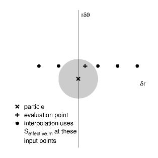
Figure 2: This figure shows our interpolation scheme for computing the 2-dimensional effective source $S_{\text{effective},m}$ near the particle. We never evaluate $S_{\text{effective},m}$ at a Euclidean distance ${}<D_{\min}$ from the particle, i.e., within the region shown as the shaded disk. Instead, for an evaluation point within this region we interpolate $S_{\text{effective},m}$ using $S_{\text{effective},m}$ values computed at more distant points.

II.9 Boundary conditions

We implement boundary conditions using finite-differencing ghost zones which lie immediately adjacent to, but outside, the nominal problem domain. At each RHS-evaluation time we first use the boundary conditions to compute $\varphi_{\text{num},m}$ and $\Pi_{\text{num},m}$ at all ghost-zone grid points. We then evaluate the RHS (and use this to time-integrate the evolution equations) at all grid points in the nominal problem domain.

II.9.1 Physical boundary conditions

We use pure outflow boundary conditions at the event horizon and ${\mathcal{J}^{+}}$, i.e., we apply the interior evolution equations at these grid points, using (conceptually) 1-sided finite difference molecules for radial derivatives.

II.9.2 $z$ axis symmetry boundary conditions

As discussed by (Barack and Golbourn, 2007, section IV.C), the $z$ axis symmetry boundary conditions for $\varphi_{\text{num},m}$ (and hence also $\Pi_{\text{num},m}$) depend on $m$.

$m=0$

In this case $\varphi_{\text{num},m}$ is even across the $z$ axis, i.e., $\partial_{\theta}\varphi_{\text{num},m}=\partial_{\theta}\Pi_{\text{num},m}=0$. The $m^{2}/\sin^{2}\theta$ term in (42) vanishes identically because $m=0$, and L’Hopital’s rule gives the other singular term as $\lim_{\theta\to 0}\cot\theta\,\partial_{\theta}\varphi_{\text{num},m}=\partial_{\theta\theta}\varphi_{\text{num},m}$.

$m\neq 0$

In this case $\varphi_{\text{num},m}$ is odd across the $z$ axis so that $\varphi_{\text{num},m}=\Pi_{\text{num},m}=0$ there. To implement this we specify zero initial data on the $z$ axis and replace our evolution equations by $\partial_{t}\varphi_{\text{num},m}=\partial_{t}\Pi_{\text{num},m}=0$ there.

II.9.3 Equatorial reflection symmetry boundary conditions

If the particle orbit is equatorial (as is the case for all the numerical computations discussed here), then the entire physical system has equatorial reflection symmetry, i.e., all fields must be even across the equator ($\theta=\pi/2$).

II.10 Initial data

The correct initial data for (25) are unknown (they would represent the equilibrium field configuration around the particle, which is what we are trying to compute). Instead, we follow the usual practice in time-domain self-force computations (e.g., Dolan and Barack (2011)) and specify arbitrary (zero) initial data $\varphi_{\text{num},m}=\Pi_{\text{num},m}=0$ on our initial slice. This initial data is not a solution of the sourced evolution equation (25), but we find that the “junk” (the deviation of the field configuration from (25)) quickly radiates away towards the inner and outer boundaries, so that after sufficient time $\varphi_{\text{num},m}$ relaxes to a solution of (25) throughout an (expanding) neighborhood of the worldtube. We see no sign of the persistent (non-radiative) “Jost junk solutions” described by Field et al. (2010a); Jaramillo et al. (2011). This is to be expected for at least two reasons: (i) the source for our field equations does not contain the derivative of a Dirac delta function, and (ii) we are using a second-order-in-space, rather than first-order-in-space formulation of the field equations.

II.11 Computing the self-force from the evolved fields

Because the physical scalar fields $\Phi$, $\Phi_{\text{puncture}}$, and $\Phi_{\text{residual}}$ are real, the Fourier inversion (15) implies that $\varphi_{-m}=\mathop{\text{conj}}\left[\varphi_{m}\right]$, and similarly for the other $m$-mode fields. Hence we only need to (numerically) compute the $m$-modes $m\geq 0$.

We thus have

$$\Phi_{\text{residual}}(t,r,\theta,\phi)=\sum_{m=0}^{\infty}\Upsilon^{(\Phi)}_{\text{residual},m}(t,r,\theta,\phi),$$ (56)

where the (real) field $\Upsilon^{(\Phi)}_{\text{residual},m}$ is given in a neighborhood of the particle by

$$\Upsilon^{(\Phi)}_{\text{residual},m} (t,r,\theta,\phi):=$$

$$\begin{cases}2\,\mathop{\text{Re}}\left[\dfrac{e^{im\tilde{\phi}}}{r}\varphi_{\text{num},m}(t,r,\theta)\right]&\text{if $m\neq 0$}\\ \dfrac{1}{r}\varphi_{\text{num},m}(t,r,\theta)&\text{if $m=0$}.\end{cases}$$ (57)

We compute the self-force by substituting (56) into (9) and differentiating at the particle position. A straightforward calculation gives

$$F_{a}=q\sum_{m=0}^{\infty}\biggl{.}\left(\Upsilon^{(\partial_{a}\Phi)}_{\text{residual},m}\right)\biggr{|}_{\text{particle}},$$ (58)

where the “self-force modes” $\Upsilon^{(\partial_{a}\Phi)}_{\text{residual},m}=\Upsilon^{(\partial_{a}\Phi)}_{\text{residual},m}(t,r,\theta)$ are defined in a neighborhood of the particle by

$$\Upsilon^{(\partial_{t}\Phi)}_{\text{residual},m} =\begin{cases}2\,\mathop{\text{Re}}\left[\dfrac{e^{im\tilde{\phi}}}{r}\Pi_{\text{num},m}\right]&\text{if $m\neq 0$}\\ \dfrac{1}{r}\Pi_{\text{num},m}&\text{if $m=0$},\end{cases}$$ (59a)

$$\Upsilon^{(\partial_{s}\Phi)}_{\text{residual},m} =\partial_{s}\Upsilon^{(\Phi)}_{\text{residual},m},$$ (59b)

$$\Upsilon^{(\partial_{\phi}\Phi)}_{\text{residual},m} =\begin{cases}-2m\,\mathop{\text{Im}}\left[\dfrac{e^{im\tilde{\phi}}}{r}\varphi_{\text{num},m}\right]&\text{if $m\neq 0$}\\ 0&\text{if $m=0$}.\end{cases}$$ (59c)

We compute each self-force mode at the particle by first computing it in a finite-difference-molecule–sized region about the particle, then interpolating it to the particle position using the “C2” interpolating function described in Appendix B.10. (For $\Upsilon^{(\partial_{s}\Phi)}_{\text{residual},m}$, an alternative would be to apply a “differentiating interpolator” directly to $\Upsilon^{(\Phi)}_{\text{residual},m}$. This would be more elegant and efficient than interpolating a molecule-sized $\Upsilon^{(\partial_{s}\Phi)}_{\text{residual},m}$ grid function. However, the cost of even the interpolate-a-molecule-size-grid-function scheme is still only a minute fraction of the overall self-force computation, so we did not bother with the additional software complexity of the differentiating interpolator.)

II.12 The tail series

In practice we can only numerically compute a finite number of $m$-modes $0\leq m\leq m_{\text{num},\max}$. We thus partition each of the infinite sums in (56) and (58) into a finite “numerical sum” plus an infinite “tail sum”,

$$\sum_{m=0}^{\infty}=\sum_{m=0}^{m_{\text{num},\max}}+\sum_{m=m_{\text{num},\max}{+}1}^{\infty},$$ (60)

and account for the tail sum in much the same way as is done in the mode-sum regularization scheme.

To estimate the tail sum for the self-force computation (58), we use the fact that the modes have a known power-law behavior that can be attributed to the non-smoothness of the residual field. Explicitly, the behavior of the modes of the residual field is given by

$$\biggl{.}\left(\Upsilon^{(\Phi)}_{\text{residual},m}\right) \biggr{|}_{\text{particle}}=$$

$$\sum_{\begin{subarray}{c}\alpha\geq n\\ \text{$\alpha$ even}\end{subarray}}k^{(\Phi)}_{\alpha}f^{(\Phi)}_{\alpha,m}+\left(\Upsilon^{(\Phi)}_{\text{regular},m}\right)\biggr{|}_{\text{particle}},$$ (61)

where $\Upsilon^{(\Phi)}_{\text{regular},m}$ comes from the $C^{\infty}$ regular field and falls off faster than any power of $m$; it can therefore be ignored for $m_{\text{num},\max}$ sufficiently large. The remaining piece of the tail sum is effectively an even power series in $1/m$, starting at an order, $m^{-n}$, that is determined by the order of the puncture field. In our case $n=4$, the basis functions $f$ for the $m$-dependence are given by

$$f^{(\Phi)}_{4,m} =\frac{1}{(m-\frac{3}{2})(m-\frac{1}{2})(m+\frac{1}{2})(m+\frac{3}{2})}$$

$$f^{(\Phi)}_{6,m} =\frac{1}{(m-\frac{5}{2})(m-\frac{3}{2})(m-\frac{1}{2})(m+\frac{1}{2})(m+\frac{3}{2})(m+\frac{5}{2})}$$

$$f^{(\Phi)}_{8,m} =\frac{1}{(m-\frac{7}{2})(m-\frac{5}{2})(m-\frac{3}{2})(m-\frac{1}{2})(m+\frac{1}{2})(m+\frac{3}{2})(m+\frac{5}{2})(m+\frac{7}{2})}$$

$$\vdots$$

$$f^{(\Phi)}_{\alpha,m} =\frac{1}{\Big{(}m-\tfrac{\alpha-1}{2}\Big{)}_{\alpha}},$$ (62)

and the coefficient functions, $k$, are given by the $m$-mode decomposition of higher-order terms (i.e., those that have not been included in the definition of the puncture field) in the series expansion of the Detweiler-Whiting singular field Heffernan et al. (2014).

Derivatives of the field behave in a similar manner, so that in addition to using this approach for $\Upsilon^{(\Phi)}_{\text{residual},m}$, we may also use it for the fields $\Upsilon^{(X)}_{\text{residual},m}$, where $X$ is one of $\partial_{s}\Phi$, $\partial_{t}\Phi$ or $\partial_{\phi}\Phi$. The only caveat is that the $m$-dependence is slightly modified: the $\phi$ derivative introduces a factor of $m^{2}$, so $f^{(\partial_{\phi}\Phi)}_{\alpha,m}=m^{2}f^{(\Phi)}_{\alpha,m}$. The $t$ derivative of the Detweiler-Whiting singular field can be written in terms of $r$ and $\phi$ derivatives, so $f^{(\partial_{t}\Phi)}_{\alpha,m}$ has both kinds of terms present.

For any given $X$, $\alpha$ and $m_{\text{num},\max}$, the infinite sum

$$S^{(X)}_{\alpha,m_{\text{num},\max}{+}1}:=\sum_{m=m_{\text{num},\max}{+}1}^{\infty}f^{(X)}_{\alpha,m}$$ (63)

can be computed exactly. Using the facts that

$$\sum_{m=-\infty}^{\infty}\Big{(}m-\tfrac{\alpha-1}{2}\Big{)}_{\alpha}=0 \qquad\text{for even $\alpha\geq 2$},$$ (64)

$$\sum_{m=-\infty}^{\infty}m^{2}\Big{(}m-\tfrac{\alpha-1}{2}\Big{)}_{\alpha}=0 \qquad\text{for even $\alpha\geq 4$},$$ (65)

we obtain

$$S^{(\Phi)}_{\alpha,m_{\text{num},\max}{+}1} =\frac{1}{(\alpha-1)\Big{(}m_{\text{num},\max}-\tfrac{\alpha-3}{2}\Big{)}_{\alpha-1}},$$ (66)

$$S^{(\partial_{\phi}\Phi)}_{\alpha,m_{\text{num},\max}{+}1} =\frac{m_{\text{num},\max}(m_{\text{num},\max}+1)}{(\alpha-3)\Big{(}m_{\text{num},\max}-\tfrac{\alpha-3}{2}\Big{)}_{\alpha-1}}.$$ (67)

Analytical expressions for the $k^{(X)}_{4}$ coefficients (in this context known as “$m$-mode regularization parameters”) compatible with our choice of puncture field were given in Heffernan et al. (2014). As they are extremely lengthy we will not repeat them here; a Mathematica notebook for computing them is included in the online supplemental materials which accompany this paper.

While the higher-order coefficients could be analytically determined in a similar manner, we choose instead an alternative approach. To estimate some finite set $\alpha\in\alpha_{\text{tail-set}}$ of the remaining $k^{(X)}_{\alpha}$ coefficients, we first truncate the series (61) to only the terms $\alpha=4$ and $\alpha\in\alpha_{\text{tail-set}}$,

$$\biggl{.}\left(\Upsilon^{(X)}_{\text{residual},m}\right)\biggr{|}_{\text{particle}}\approx k^{(X)}_{4}f^{(X)}_{4,m}+\sum_{\begin{subarray}{c}\text{$\alpha$ even}\\ \alpha\in\alpha_{\text{tail-set}}\end{subarray}}k^{(X)}_{\alpha}f^{(X)}_{\alpha,m}.$$ (68)

For a specified particle position, we then estimate the corresponding set of $k^{(X)}_{\alpha}$ by least-squares fitting the numerically-computed $\biggl{.}\left(\Upsilon^{(X)}_{\text{residual},m}\right)\biggr{|}_{\text{particle}}$ with $m_{\mathop{\text{fit}},\min}\leq m\leq m_{\mathop{\text{fit}},\max}$ to the truncated series (68). For all analyses reported in this paper we take $\alpha_{\text{tail-set}}$ to be either empty (no tail fit) or $\{6,8\}$. Table 3 gives $m_{\mathop{\text{fit}},\min}$ and $m_{\mathop{\text{fit}},\max}$ for each of our configurations where a tail fit is done.

Finally, we compute (estimate) each self-force component $F_{a}$ at each of these times by substituting (60), (61), and (63) into (58), giving

$$\frac{F_{a}}{q}={} \sum_{m=0}^{m_{\text{num},\max}}\biggl{.}\left(\Upsilon^{(X)}_{\text{residual},m}\right)\biggr{|}_{\text{particle}}$$

$${}+k^{(X)}_{4}S^{(X)}_{4,m_{\text{num},\max}{+}1}$$

$${}+\sum_{\begin{subarray}{c}\text{$\alpha$ even}\\ \alpha\in\alpha_{\text{tail-set}}\end{subarray}}k^{(X)}_{\alpha}S^{(X)}_{\alpha,m_{\text{num},\max}{+}1}.$$ (69)

II.13 Selecting the time interval for analysis within an evolution

Our discussion in sections II.11 and II.12 assumed that a time series of the self-force modes $\Upsilon^{(\partial_{a}\Phi)}_{\text{residual},m}$ is available at a suitable set of points around the orbit for each $m=0$, $1$, $2$, …, $m_{\text{num},\max}$. However, as described in section II.10, the initial part of each such time series is contaminated by “junk” radiation. Here we describe how we determine when this junk radiation has decayed to a negligible level (below our numerical noise level).

The key fact which underlies our algorithm for making this determination is that since the particle orbit is periodic, the self-force modes should also be periodic with the orbital period $T_{r}$..

Given a time series of some numerically-computed self-force mode $\Upsilon^{(\partial_{a}\Phi)}_{\text{residual},m}$, we define its “orbit difference” time series by

$$\Delta\left[\Upsilon^{(\partial_{a}\Phi)}_{\text{residual},m}\right]\!(t):=\left|\Upsilon^{(\partial_{a}\Phi)}_{\text{residual},m}(t+T_{r})-\Upsilon^{(\partial_{a}\Phi)}_{\text{residual},m}(t)\right|.$$ (70)

The orbit-difference time series is one orbit shorter in duration than the original time series.

Because of the initial junk radiation, the orbit difference is initially large. As the junk radiation radiates away from the particle and worldtube, the orbit difference decays until it eventually becomes roughly constant (at a nonzero value due to finite differencing and other numerical errors) or, in some cases, varying with the orbital period (since the numerical errors are similarly periodic). (This behavior can be seen in Fig. 3.)

It is thus quite easy to determine the time when the junk radiation has decayed to a negligible level by visually inspecting a graph of the orbit difference as a function of time. Although this process could probably be automated by searching backwards in the orbit-difference time series for a sustained rise (in fact, we implemented such an algorithm), we find that the visual inspection is valuable for detecting a variety of other numerical problems which might occur, so we have chosen not to routinely use an automated algorithm here.

II.14 Selecting a “low-noise” subset of times within an evolution

Because of the interaction between finite differencing and the limited differentiability of $\varphi_{\text{num}}$ at the particle, as well as other numerical errors, there is numerical noise in the self-force modes $\Upsilon^{(\partial_{a}\Phi)}_{\text{residual},m}$. For highly eccentric orbits, we find that the higher-$m$ modes may be completely dominated by numerical noise in the outer parts of the orbit. (This can be seen in, for example, Figs. 4 and 5.)

Including these modes in the self-force sum (69) would add significant numerical noise to the computed self-force while (in many cases) not adding any significant “signal”. Therefore, it is useful (again, in many although not all cases) to omit the noisy modes from the self-force sum (69), effectively treating these modes/times as missing data.

To estimate the noise level at any point in an $\Upsilon^{(\partial_{a}\Phi)}_{\text{residual},m}$ time series, we first define a smoothed time series $\mathcal{S}\left[\Upsilon^{(\partial_{a}\Phi)}_{\text{residual},m}\right]$ using Savitzky-Golay moving-window smoothing Savitzky and Golay (1964), (Press et al., 2007, section 14.8). For all analyses reported in this paper we use a 6th-degree polynomial over a $\text{current position}\pm 10$-sample moving window in the time series.

We then define the (absolute) noise time series as

$$\text{noise}\left[\Upsilon^{(\partial_{a}\Phi)}_{\text{residual},m}\right]\!(t):=$$

$$\qquad\mathop{\text{RMS}}_{\text{SG window}(t)}\biggl{\{}\Upsilon^{(\partial_{a}\Phi)}_{\text{residual},m}-\mathcal{S}\left[\Upsilon^{(\partial_{a}\Phi)}_{\text{residual},m}\right]\biggr{\}}$$ (71)

and the “relative noise” time series as

$$\text{relative\_noise}\left[\Upsilon^{(\partial_{a}\Phi)}_{\text{residual},m}\right]\!(t):=$$

$$\qquad\text{noise}\left[\Upsilon^{(\partial_{a}\Phi)}_{\text{residual},m}\right]\!(t)\Bigg{/}\mathop{\text{RMS}}_{\text{SG window}(t)}\Bigl{\{}\Upsilon^{(\partial_{a}\Phi)}_{\text{residual},m}\Bigr{\}},$$ (72)

where $\displaystyle\mathop{\text{RMS}}_{\text{SG window}(t)}\bigl{\{}\cdots\bigr{\}}$ is the root-mean-square value over the Savitzky-Golay smoothing window.

Using these definitions we select a “low-noise” subset of the time samples by omitting those samples from the $\Upsilon^{(\partial_{a}\Phi)}_{\text{residual},m}$ time series which have $m\geq m_{\text{noise},\min}$ and $\text{relative\_noise}\left[\Upsilon^{(\partial_{a}\Phi)}_{\text{residual},m}\right]>\varepsilon_{\text{relative},\max}$, where $m_{\text{noise},\min}$ is a parameter chosen so that time intervals immediately around zero-crossings in lower-$m$ modes are not falsely excluded, and where $\varepsilon_{\text{relative},\max}$ is a parameter chosen to tune the tolerable level of numerical noise. Table 3 gives $m_{\text{noise},\min}$ and $\varepsilon_{\text{relative},\max}$ for each of our configurations where smoothing is done.

II.15 Dissipative and conservative parts of the self-force

As well as calculating the overall self-force, it is useful to split the self-force into dissipative and conservative contributions Mino (2003); Hinderer and Flanagan (2008); Diaz-Rivera et al. (2004); Barack and Sago (2009); Vega et al. (2013): the dissipative part affects the $\mathcal{O}(\mu)$ orbital evolution while the conservative part only affects the orbital evolution at $\mathcal{O}(\mu^{2})$. As discussed by (Barack, 2009, section 8.1), for equatorial orbits these can be computed from the even-in-time and odd-in-time parts of the self-force,

$$F_{\text{diss},t} =F_{\text{even},t} F_{\text{cons},t} =F_{\text{odd},t}$$ (73a)

$$F_{\text{diss},r} =F_{\text{odd},r} F_{\text{cons},r} =F_{\text{even},r}$$ (73b)

$$F_{\text{diss},\phi} =F_{\text{even},\phi} F_{\text{cons},\phi} =F_{\text{odd},\phi}$$ (73c)

where

$$F_{\text{even},a}(t) =\tfrac{1}{2}\bigl{[}F_{a}(t)+F_{a}(T_{r}-t)\bigr{]}$$ (74a)

$$F_{\text{odd},a}(t) =\tfrac{1}{2}\bigl{[}F_{a}(t)-F_{a}(T_{r}-t)\bigr{]}$$ (74b)

with $t$ being the modulo time.

To allow this computation without requiring time interpolation, we always choose our self-force computation times to be uniformly spaced in coordinate time $t$, with a spacing $\Delta t_{\text{sample}}$ which integrally divides the orbital period $T_{r}$.

II.16 Summary of computation and data analysis

To summarize, our overall computational and data-analysis scheme involves a sequence of operations:

• For each $m$, we perform a numerical evolution of the 1st-order-in-time evolution system described in section II.6. Our evolution code writes out time series of each self-force mode $\Upsilon^{(\partial_{a}\Phi)}_{\text{residual},m}$, sampled at uniform coordinate-time intervals. We always choose the sampling time $\Delta t_{\text{sample}}$ to be the same for each $m$ and (as noted in section II.15) to integrally divide the period $T_{r}$ of the particle’s radial motion.

• For each $m$, we use the orbit-differences algorithm described in section II.13 to select a point in each of the self-force modes’ time series when the initial junk radiation has decayed to a level below our numerical noise level. For all our further data analysis we use only the modes from times $\geq$ this “self-force computation start time” for each $m$.

• For most configurations, for each $m$ we use the noise-estimation and low-noise–selection algorithms described in section II.14 to select a subset of the self-force mode $\Upsilon^{(\partial_{a}\Phi)}_{\text{residual},m}$ time series which has relatively low numerical noise.

• For each modulo time for which we have self-force modes (at times $\geq$ the self-force computation start time, and with sufficiently low estimated noise), we compute the $t$, $r$, and $\phi$ components of the self-force using the mode summation and tail-fitting algorithms described in sections II.11 and II.12.

III Numerical results

III.1 Configurations and parameters

Tables 1–8 summarize the main physical and computational parameters for the configurations presented here. These configurations fall into four (overlapping) families:

• The ns5, n-55, n95, ze4, and e8b configurations are ones which have also been calculated by other researchers, allowing us to validate our code against their results (both published and unpublished).

• The e8, e8b, e9, and e95 configurations are (non–zoom-whirl) highly eccentric orbits.

• The ze4, ze9, zze9, and ze98 configurations are zoom-whirl orbits; of these the ze4 configuration is of moderate eccentricity while the ze9, zze9, and ze98 configurations are highly eccentric.

• The circ-ze4, circ-ze9, circ-zze9, and circ-ze98 configurations are circular-orbit configurations with orbital radii matching the periastrons of the corresponding zoom-whirl configurations.

								Orbital period			$\delta\phi$ per
						min $r$	max $r$	Radial		Azimuthal	orbit
Name	$\tilde{a}$	$p$	$e$	$\mathcal{E}$ ($M$)	$\mathcal{L}$ ($M^{2}$)	($M$)	($M$)	$T_{r}$ ($M$)	$\tau_{r}$ ($M$)	$T_{\phi}$ ($M$)	(orbits)
ns5	$0.0$	$7.2$	$0.5$	0.956 876	3.622 713	$4.8$	$14.4$	$405.662$	$317.366$	$134.285$	$3.021$
n-55	$-0.5$	$10.0$	$0.5$	0.967 896	4.100 631	$6.667$	$20.0$	$505.428$	$434.465$	$249.488$	$2.026$
n95	$0.9$	$10.0$	$0.5$	0.963 778	3.489 553	$6.667$	$20.0$	$378.408$	$333.027$	$293.070$	$1.291$
e8	$0.6$	$8.0$	$0.8$	0.978 270	3.405 897	$4.444$	$40.000$	$771.968$	$709.796$	$502.435$	$1.536$
e8b	$0.8$	$8.0$	$0.8$	0.978 056	3.292 113	$4.444$	$40.000$	$756.641$	$697.570$	$527.812$	$1.434$
e9	$0.99$	$7.0$	$0.9$	0.986 565	3.052 860	$3.684$	$70.000$	$1513.855$	$1442.724$	$1060.526$	$1.427$
e95	$0.99$	$5.0$	$0.95$	0.990 315	2.699 644	$2.564$	$100.000$	$2436.050$	$2349.870$	$1445.400$	$1.685$
ze4	$0.2$	$6.15$	$0.4$	0.945 536	3.366 468	$4.393$	$10.25$	$354.628$	$255.966$	$95.799$	$3.702$
ze9	$0.0$	$7.800\,1$	$0.9$	0.988 333	3.904 885	$4.105$	$78.001$	$2112.079$	$1913.402$	$339.855$	$6.215$
zze9	$0.0$	$7.800\,001$	$0.9$	0.988 332	3.904 884	$4.105$	$78.000$	$2224.815$	$1971.883$	$265.734$	$8.372$
ze98	$0.99$	$2.4$	$0.98$	0.991 798	2.180 959	$1.212$	$120.000$	$3304.620$	$3021.480$	$215.851$	$15.310$
circ-ze4	$0.2$	$4.392\,857$	$0.0$	0.943 384	3.346 263	$4.392\,857$	$4.392\,857$			$59.106$
circ-ze9	$0.0$	$4.105\,316$	$0.0$	0.988 327	3.904 841	$4.105\,316$	$4.105\,316$			$52.264$
circ-zze9	$0.0$	$4.105\,264$	$0.0$	0.988 332	3.904 884	$4.105\,264$	$4.105\,264$			$52.263$
circ-ze98	$0.99$	$1.212\,121$	$0.0$	0.984 732	2.164 538	$1.212\,121$	$1.212\,121$			$14.605$

Table 1: This table summarizes the main physical parameters for the configurations presented in this paper. $(\tilde{a},p,e)$ uniquely characterize the spacetime and the particle orbit. $\mathcal{E}$ and $\mathcal{L}$ are the particle’s specific energy and angular momentum, respectively. “min $r$” and “max $r$” are the particle’s periastron and apoastron coordinate radii, respectively. The orbital period is given in three forms: the coordinate time $T_{r}$ and proper time along the particle orbit $\tau_{r}$ of the radial motion, and the long-term mean coordinate-time period $T_{\phi}$ of the azimuthal ($\phi$) motion (i.e., the mean coordinate time $t$ during which $\phi$ advances by $2\pi$). “$\delta\phi$ per orbit” denotes the advance in $\phi$ (in units of $2\pi$) during one period of the orbit’s radial motion (i.e., during a coordinate time $T_{r}$); this is given by $T_{r}/T_{\phi}$ and is $\gg 1$ orbit for a zoom-whirl orbit.

					Self-force computation start time					Evolution end time
		$\Delta t_{\text{sample}}$		$t_{\text{initial}}$	$m=0$	$m=1$	$m=2$	$m=3$	$m\geq 4$	$m=0$	$m=1$	$m=2$	$m=3$	$m\geq 4$
Name	$N_{\text{sample}}$	($M$)	$m_{\text{num},\max}$	($M$)	($M$)	($M$)	($M$)	($M$)	($M$)	($M$)	($M$)	($M$)	($M$)	($M$)
ns5	00 406	0.999	20	143	8 000	2 000	700	365	310	11 990	6 994	3 997	1 349	1 349
n-55	00 506	0.999	20	183	7 200	2 700	900	480	420	10 291	5 237	3 721	1 348	1 348
n95	00 378	1.001	20	116	5 115	2 850	890	400	350	12 013	8 009	4 004	1 251	1 251
e8	00 770	1.003	20	324	7 000	2 600	1 300	800	650	11 903	6 500	4 184	2 506	2 506
e8b	00 760	0.996	20	289	8 700	4 200	1 900	1 025	820	11 728	7 945	5 675	3 405	3 405
e9	1 514	1.000	20	680	10 000	5 300	2 450	1 300	1 180	15 818	8 249	5 221	3 300	3 300
e95	2 436	1.000	20	1 090	7 000	4 700	2 550	2 200	1 950	13 270	8 398	5 962	5 400	5 400
ze4	00 360	0.985	20	111	8 000	2 000	550	400	360	11 821	6 896	3 940	1 182	1 182
ze9	2 112	1.000	20	920	12 888	7 888	2 500	1 600	1 600	15 001	10 000	8 000	4 800	4 800
zze9	2 224	1.000	20	1 005	10 000	5 550	3 350	1 700	1 575	22 361	14 461	12 236	7 787	7 787
ze98	13 216	0.250	12	1 448	11 600	8 250	4 950	4 950	4 950	18 093	14 871	14 871	13 218	10 623
circ-ze4	00 060	0.982	20	0	6 000	2 000	450	315	300	6 154	4 000	940	700	600
circ-ze9	00 052	1.005	20	0	10 000	1 630	410	325	335	10 453	1 980	950	685	425
circ-zze9	00 052	1.005	20	0	10 000	1 630	410	325	335	10 453	1 980	950	685	425

Table 2: For each configuration, this table gives the number of self-force output samples per orbit (more precisely, per radial orbital period for the eccentric-orbit configurations, and per azimuthal orbital period for the circular-orbit configurations), the sampling interval, the maximum $m$ of the numerically-computed modes in the self-force sum (69), the time at which the self-force computation begins (after the initial transients have decayed), and the time at which the numerical evolution ends (or at which the self-force computation ends, if this is earlier). All times are coordinate times in units of $M$ and (except for $\Delta t_{\text{sample}}$) are rounded to the nearest integer. For some configurations (footnoted), some large-$m$ evolutions use earlier starting and/or ending times (chosen to select low–numerical-noise sections of data and/or limited by machine failures or queue-time limits). For the eccentric-orbit configurations there is always at least one orbital period between the starting and ending times; for the circular-orbit configurations the self-force is time-independent so there is no need for an extended self-force computation interval. The circ-ze98 configuration is omitted because we were unable to obtain stable evolutions for it for $m\geq 6$.

	low-noise selection
	parameters		tail-fit parameters
Name	$m_{\text{noise},\min}$	$\varepsilon_{\text{relative},\max}$	$m_{\mathop{\text{fit}},\min}$	$m_{\mathop{\text{fit}},\max}$
ns5	10	0.05	09	18
n-55	10	0.05	09	18
n95	10	0.05	09	18
e8	04	0.30	12	20
e8b	04	0.30	12	20
e9	03	0.30	12	20
e95	02	0.30	12	20
ze4	10	0.05	08	18
ze9	02	0.30	12	20
zze9	02	0.30	12	20
ze98	no low-noise selection		— no tail fit —
circ-ze4	no low-noise selection		12	20
circ-ze9	no low-noise selection		12	20
circ-zze9	no low-noise selection		12	20

Table 3: This table shows the low-noise–selection and tail-fit parameters used for computing the self-force for each configuration presented in this paper. The circ-ze98 configuration is omitted because we were unable to obtain stable evolutions for it for $m\geq 6$.

	Numerical grid
	dro4-32	dro6-48	dro6-48	dro8-64	dro10-80
Name	normal	normal	variant	normal	normal
ns5	✓	✓		✓
n-55	✓	✓
n95	✓	✓		✓
e8	✓	✓		✓
e8b	✓	✓
e9	✓	✓	✓	✓	✓
e95	✓	✓		✓
ze4	✓	✓
ze9	✓	✓
zze9	✓	✓		✓
ze98	✓	✓		✓	✓
circ-ze4	✓			✓
circ-ze9	✓			✓
circ-zze9	✓			✓
circ-ze98	✓			✓

Table 4: This table shows which numerical grids were used in simulating the configurations presented in this paper. See tables 5 and 6 for details of these grids.

		base grid		finest grid
		$R_{*}$	$\theta$	$R_{*}$	$\theta$
		($M$)	(radians)	($M$)	(radians)
dro4-32	normal	$1/4$	$\pi/72\phantom{0}$	$1/32$	$\pi/576\phantom{0}$
dro6-48	normal	$1/6$	$\pi/108$	$1/48$	$\pi/864\phantom{0}$
dro6-48	variant	$1/6$	$\pi/96\phantom{0}$	$1/48$	$\pi/768\phantom{0}$
dro8-64	normal	$1/8$	$\pi/144$	$1/64$	$\pi/1152$
dro10-80	normal	$1/1\hbox to0.0pt{0\hss}$	$\pi/180$	$1/80$	$\pi/1440$

Table 5: This table shows the range of grid resolutions used for each of our standard grid structures. Each grid structure has a base grid and 3 refined grids, with a 2:1 refinement ratio between adjacent refinement levels. See table 6 for the sizes and shapes of each refinement level.

			$R_{*}$		$\theta$
	refinement	moves with	min	max	min	max
grid type	level	worldtube?			(radians)	(radians)
normal	0	no	$R_{*}^{h}$	$R_{*}^{\mathcal{J}^{+}}$	$0$	$\pi/2$
	1	yes	$\texttt{WT\_center}-30\,M$	$\texttt{WT\_center}+30\,M$	$0$	$\pi/2$
	2	yes	$\texttt{WT\_center}-15\,M$	$\texttt{WT\_center}+15\,M$	$\pi/4$	$\pi/2$
	3	yes	$\texttt{WT\_center}-\phantom{0}{}8\,M$	$\texttt{WT\_center}+\phantom{0}{}8\,M$	$\pi/3$	$\pi/2$
variant	0	no	$R_{*}^{h}$	$R_{*}^{\mathcal{J}^{+}}$	$0$	$\pi/2$
	1	yes	$\texttt{WT\_center}-35\phantom{.0}\,M$	$\texttt{WT\_center}+40\phantom{.0}\,M$	$0$	$\pi/2$
	2	yes	$\texttt{WT\_center}-18\phantom{.0}\,M$	$\texttt{WT\_center}+18\phantom{.0}\,M$	$5\pi/24$	$\pi/2$
	3	yes	$\texttt{WT\_center}-\phantom{0}{}6.5\,M$	$\texttt{WT\_center}+\phantom{0}{}7.5\,M$	$5\pi/16$	$\pi/2$

Table 6: This table shows the size and shape of each refinement level in our numerical grids. WT_center is the $R_{*}$ coordinate of the worldtube center. See table 5 for the grid resolutions.

Initial startup
initial time ($t_{\text{initial}}$)	$323.825$	$M$
particle $R_{*}$ at initial time	$45.016$	$M$
particle apoastron time	$385.984$	$M$
particle $R_{*}$ at apoastron	$45.889$	$M$
time of first worldtube move ($m=2$)	$448.706$	$M$
particle $R_{*}$ at time of first worldtube move	$45.000$	$M$
time interval from initial time to first worldtube move ($m=2$)	$124.881$	$M$
Worldtube
$R_{*}$ (radial) radius (WT_radius)	$5.0$	$M$
$\theta$ (angular) radius	$\pi/8$	radians
initial value of worldtube center $R_{*}$ (WT_center)	$45.5$	$M$
worldtube center $\theta$	$\pi/2$	radians
move worldtube if $\bigl{|}\text{particle $R_{*}$}-\texttt{WT\_center}\bigr{|}>f_{\text{move}}\times\texttt{WT\_radius}$, where $f_{\text{move}}=\dots$
initial startup	$0.10$
main evolution	$0.05$
when moving worldtube, place new worldtube center ahead of particle $R_{*}$
(where “ahead” is defined based on sign of particle $R_{*}$ 3-velocity)
by $f_{\text{ahead}}\times f_{\text{move}}\times\texttt{WT\_radius}$, where $f_{\text{ahead}}=\dots$	$0.9$
$\text{maximum $R_{*}$ distance to move worldtube at any one time}=f_{\text{max-move}}\times\texttt{WT\_radius}$, where $f_{\text{max-move}}=\dots$	$0.1$
minimum time interval between worldtube moves	$1.0$	$M$
Overall evolution
number of worldtube moves per orbit	$164$

Table 7: This table summarizes miscellaneous computational parameters for the e8 runs.

	particle motion		compactification
Name	$\min$ $R_{*}$	$\max$ $R_{*}$	$R_{*}^{h}$	$R_{*}^{-}$	$R_{*}^{+}$	$R_{*}^{\mathcal{J}^{+}}$
	($M$)	($M$)	($M$)	($M$)	($M$)	($M$)
ns5	$4.8$	$14.4$	-70	-45	+70	+95
n-55	$8.370$	$24.395$	-70	-45	+75	+100
n95	$8.390$	$24.397$	-70	-45	+75	+100
e8	$4.884$	$45.889$	-75	-50	+125	+150
e8b	$4.884$	$45.889$	-75	-50	+125	+150
e9	$3.524$	$77.053$	-75	-50	+160	+185
e95	$0.782$	$107.784$	-75	-50	+190	+215
ze4	$4.756$	$13.085$	-70	-45	+65	+90
ze9	$4.208$	$85.276$	-75	-50	+135	+160
zze9	$4.208$	$85.275$	-75	-50	+135	+160
ze98	$-15.227$	$120.000$	-90	-65	+180	+205
circ-ze4	$4.756$	$4.756$	-70	-45	+55	+80
circ-ze9	$4.208$	$4.208$	-70	-45	+55	+80
circ-zze9	$4.208$	$4.208$	-70	-45	+55	+80
circ-ze98	$-15.227$	$-15.227$	-90	-65	+50	+75

Table 8: This table summarizes the compactification parameters for the configurations presented in this paper.

III.2 Example of data analysis

Here we give an example of the data analysis “pipeline” described in section II.16, for the e8 configuration, which has $(\tilde{a},p,e)=(0.6,8,0.8)$.

Figure 3 shows a selection of the modes $\Upsilon^{(\partial_{r}\Phi)}_{\text{residual},m}$ and their orbit differences $\Delta\left[\Upsilon^{(\partial_{r}\Phi)}_{\text{residual},m}\right]$ for the entire time span of each $m$’s evolution. Figure 4 shows all of the $\Upsilon^{(\partial_{r}\Phi)}_{\text{residual},m}$ for the last $2.85$ orbital periods for each $m\in[0,20]$ for the e8 configuration. Figure 5 shows a selection of the modes $\Upsilon^{(\partial_{a}\Phi)}_{\text{residual},m}$ in more detail as a function of modulo time.

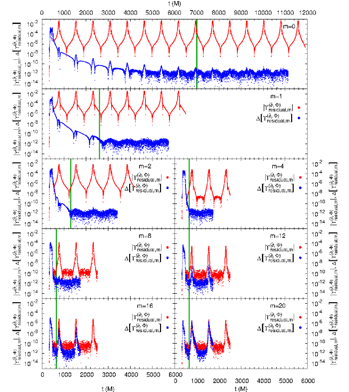
Figure 3: This figure shows some of the self-force modes $\Upsilon^{(\partial_{r}\Phi)}_{\text{residual},m}$ and their orbit differences $\Delta\left[\Upsilon^{(\partial_{r}\Phi)}_{\text{residual},m}\right]$ for the e8 configuration, which has $(\tilde{a},p,e)=(0.6,8,0.8)$. In each subplot the green vertical line marks the self-force computation starting time (when the orbit differences have decayed to the numerical noise level). For each $m$ the orbit differences are only defined for a time interval that is one orbital period shorter than the self-force mode. As $m$ increases the initial junk decays faster, so the self-force computation starting time can be earlier in the evolution. Correspondingly, we choose shorter numerical evolutions for larger $m$.

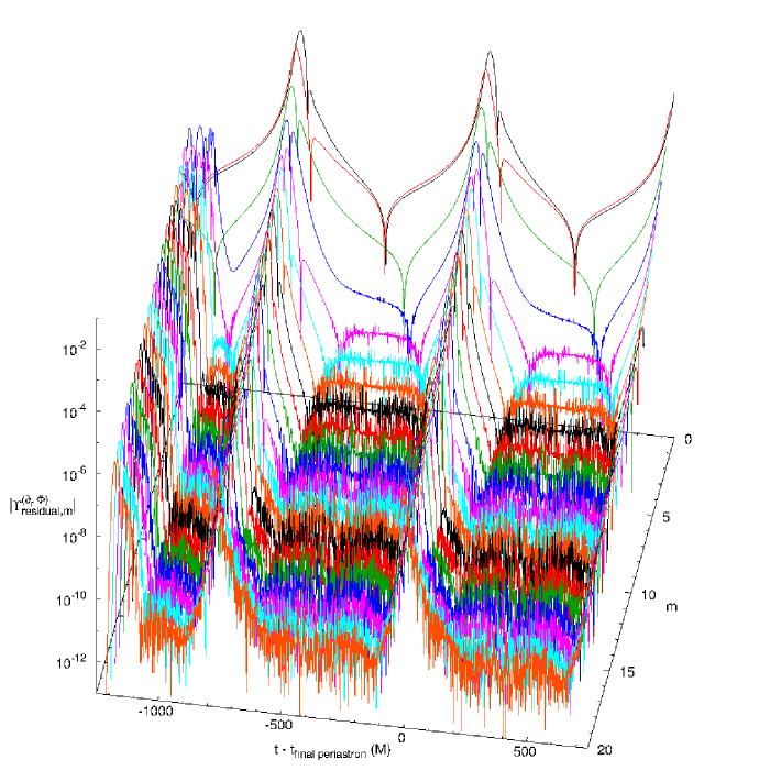
Figure 4: This figure shows all of our numerically-computed self-force modes $\Upsilon^{(\partial_{r}\Phi)}_{\text{residual},m}$ for the last $2.6$ orbital periods for each $m\in[0,20]$ for the e8 configuration, which has $(\tilde{a},p,e)=(0.6,8,0.8)$. Compare these with the “low-noise” subset of modes shown in Fig. 6.

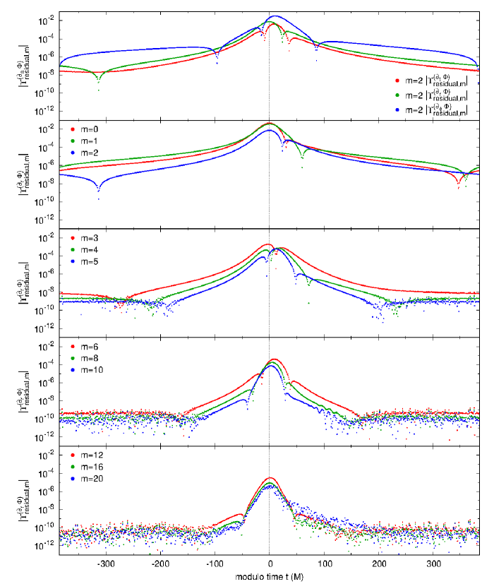
Figure 5: This figure shows some of the self-force modes $\Upsilon^{(\partial_{a}\Phi)}_{\text{residual},m}$ for the e8 configuration, which has $(\tilde{a},p,e)=(0.6,8,0.8)$. The figure shows only data for the final orbit simulated for each $m$. Compare these modes with the “low-noise” subset of modes shown in Fig. 7.

After applying the “low-noise” selection criteria described in section II.14, Fig. 6 shows the resulting “low-noise” subset of the $\Upsilon^{(\partial_{r}\Phi)}_{\text{residual},m}$ for the last $2.6$ orbital periods for each $m\in[0,20]$ for the e8 configuration, and Fig. 7 shows a selection of the low-noise modes $\Upsilon^{(\partial_{a}\Phi)}_{\text{residual},m}$ in more detail as a function of modulo time. We use these modes to compute the self-force using the mode summation and tail-fitting algorithms described in sections II.11 and II.12.

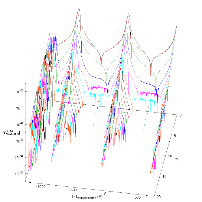
Figure 6: This figure shows the “low-noise” numerically-computed self-force modes $\Upsilon^{(\partial_{r}\Phi)}_{\text{residual},m}$ for the last $2.6$ orbital periods for each $m\in[0,20]$ for the e8 configuration, which has $(\tilde{a},p,e)=(0.6,8,0.8)$. Compare these with the full set of modes shown in Fig. 4.

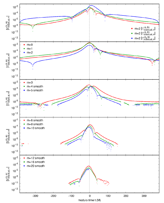
Figure 7: This figure shows some of the “low-noise” self-force modes $\Upsilon^{(\partial_{a}\Phi)}_{\text{residual},m}$ for the final orbit for each $m$ for the e8 configuration, which has $(\tilde{a},p,e)=(0.6,8,0.8)$. Compare these modes with the full set of modes shown in Fig. 5.

Figure 8 shows some example tail fits of the low-noise modes $\Upsilon^{(\partial_{r}\Phi)}_{\text{residual},m}$ to the tail series (69) for the n95 and e8 configurations.

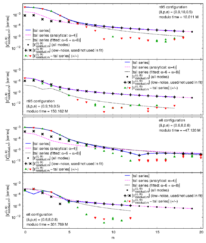
Figure 8: This figure shows sample fits of the numerically computed $\Upsilon^{(\partial_{r}\Phi)}_{\text{residual},m}$ to the tail series (69) for selected times in the n95 and e8 configurations. The tail series, fitted tail series, and tail series difference $\bigl{|}\Upsilon^{(\partial_{a}\Phi)}_{\text{residual},m}-\text{tail series}\bigr{|}$ are only shown for the low-noise modes. For this difference, $\blacktriangle$ or $\blacktriangledown$ means $\Upsilon^{(\partial_{a}\Phi)}_{\text{residual},m}-\text{tail series}>0$ or $<0$, respectively.

III.3 Convergence of results with numerical resolution

When numerically solving partial differential equations, the results should (must!) converge to a continuum limit. More precisely (for finite-difference computations), as the grid is refined, at each event the results should in general be convergent with the correct convergence order for the finite differencing scheme Choptuik (1991). However, our numerical scheme is an exception: as the particle moves through the grid, the limited differentiability of our numerical fields at the particle position introduces finite differencing errors which fluctuate in a “bump function” manner (Thornburg, 1999, appendix F) from one particle position to another. Moreover, these fluctuations are typically not coherent between different-resolution evolutions. Correspondingly, we expect the convergence of our numerical results to fluctuate from one modulo-time (orbital position) sample to the next.

Figure 9 illustrates this fluctuating convergence for the n95 and e9 configurations. As expected, the self-force difference norms $\bigl{\|}F_{a}^{(\text{low})}\,{-}\,F_{a}^{(\text{high})}\bigr{\|}_{+}$ and the convergence ratio $\bigl{\|}F_{a}^{(\text{low})}\,{-}\,F_{a}^{(\text{medium})}\bigr{\|}_{+}\Big{/}\bigl{\|}F_{a}^{(\text{medium})}\,{-}\,F_{a}^{(\text{high})}\bigr{\|}_{+}$ fluctuate strongly (typically by an order of magnitude or more) from one sample to the next. This makes it difficult to accurately estimate an overall order of convergence. However, several conclusions can be drawn:

• For both configurations there is no systematic difference in the convergence ratio between the ingoing and outgoing legs of the orbit at any given radius $r$.

• For the n95 configuration the convergence order is roughly similar everywhere in the orbit, averaging somewhat better than 2nd order.

• For the e9 configuration the convergence averages much better than 4th order for $r\lesssim 10\,M$, somewhat worse than 2nd order for $10\,M\lesssim r\lesssim 20\,M$, and roughly 4th order for $r\gtrsim 25\,M$.

  We have not yet been able to determine the reason for this somewhat peculiar convergence behavior. However, since our overall finite differencing scheme is 4th order accurate (in both space and time) in the bulk, achieving an average convergence higher than this implies that one or more of the (e9) evolutions must have insufficient resolution to be in the asymptotic-convergence regime.

  Our grid structure for these evolutions (Tab. 6) moves the finest 3 refinement levels with the worldtube, which in turn moves so that its center is always very close to the particle. Thus, if the particle is at a sufficiently large radius the strong-field region close to the black hole will not be covered by the finest grid. For example, if the particle is at $r\,{=}\,R\,{=}\,10\,M$ ($R_{*}=12.8\,M$) then the finest grid extends inward only as far as $r\,{=}\,R\,{=}\,4.4\,M$ ($R_{*}\,{=}\,4.8\,M$). For phenomena nearer the black hole than this, the local grid resolution is lower. As we discuss in section IV.2.3, an adaptive mesh-refinement scheme might well provide improved accuracy – and convergence – in this situation.

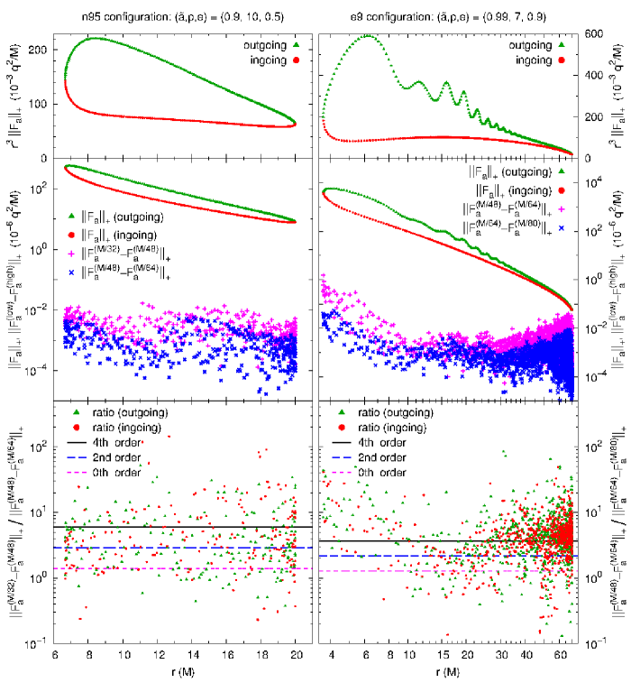
Figure 9: This figure shows the convergence of the self-force with numerical resolution for the n95 and e9 configurations. For the n95 configuration the convergence is calculated using the dro4-32, dro6-48, and dro8-64 numerical grids (labelled by their finest $\Delta R_{*}$ of $M/32$, $M/48$, and $M/64$ respectively), while for the e9 configuration the convergence is calculated using the dro6-48, dro8-64, and dro10-80 numerical grids (labelled by their finest $\Delta R_{*}$ of $M/48$, $M/64$, and $M/80$ respectively). The top subplots in each column shows the configuration’s self-force loop for the positive-definite pointwise norm of the self-force, $\|F_{a}\|_{+}$. The middle subplots show the difference norms $\bigl{\|}F_{a}^{(\text{low})}\,{-}\,F_{a}^{(\text{medium})}\bigr{\|}_{+}$ and $\bigl{\|}F_{a}^{(\text{medium})}\,{-}\,F_{a}^{(\text{high})}\bigr{\|}_{+}$. The bottom subplots show the convergence ratios $\bigl{\|}F_{a}^{(\text{low})}\,{-}\,F_{a}^{(\text{medium})}\bigr{\|}_{+}\Big{/}\bigl{\|}F_{a}^{(\text{medium})}\,{-}\,F_{a}^{(\text{high})}\bigr{\|}_{+}$ (plotted separately for the ingoing and outgoing legs of the orbit), along with the theoretical values of this ratio for 0th, 2nd, and 4th order convergence. Notice that there is no systematic difference in the convergence ratios between the ingoing (red symbols) and outgoing (green symbols) legs of the orbit.

On a more qualitative level, figure 23 shows visually that the difference between our highest and 2nd-highest resolution results is very small for the near-periastron parts of the ze4, ze9, and zze9 orbits.

III.4 Verification that results are independent of the choice of worldtube and other numerical parameters

As discussed in section II.3, our numerically computed self-force should be independent of the choice of the worldtube. To test this independence numerically, we compare results for the e9 configuration computed using the normal and variant dro6-48 numerical grids (these are described in detail in tables 5 and 6). As well as varying the sizes and positions of each refined grid, these computations also use different $\Delta R_{*}\big{/}\Delta\theta$ grid aspect ratios (table 5), different worldtube sizes, and different worldtube-moving parameters $f_{\text{move}}$ and max_move_distance (these parameters are defined in figure 26). Figure 10 shows a numerical comparison of the self-force between these computations. It is apparent that changing these parameters changes the computed self-force by only a very small amount (similar in size to the change induced by a factor-of-$1.5$ change in numerical resolution).

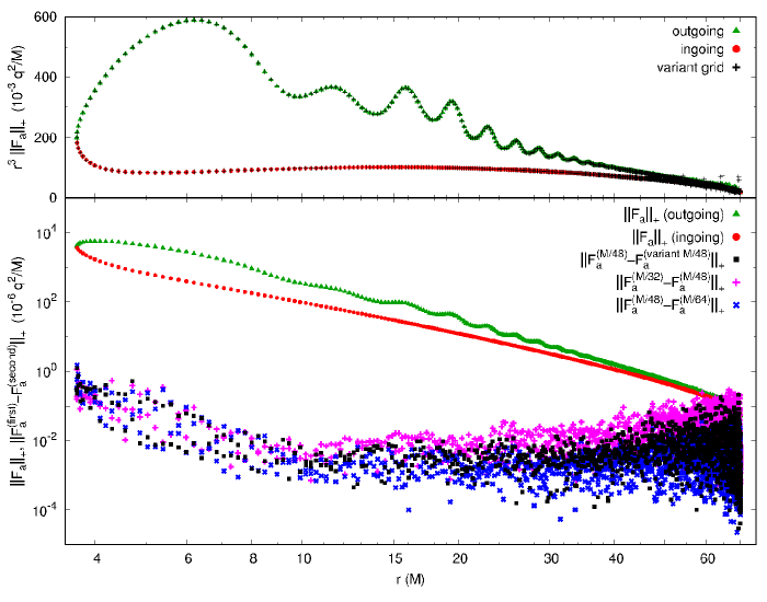
Figure 10: This figure shows a numerical verification that our computed self-force is (approximately) independent of the choice of worldtube and other numerical parameters, for the e9 configuration (which has $(\tilde{a},p,e)=(0.99,7,0.9)$). The top subplot shows the self-force loop for the positive-definite pointwise norm of the self-force, $\|F_{a}\|_{+}$, with computations using the dro6-48 and variant dro6-48 worldtube/grids overplotted. The points all coincide visually to high accuracy. The bottom subplot shows a quantitative assessment, the norm of the change in the self-force between the dro6-48 and variant dro6-48 worldtube/grid computations, $\bigl{\|}F_{a}^{(M/48)}\,{-}\,F_{a}^{(\text{variant $M/48$})}\bigr{\|}_{+}$, together with the change-in-resolution difference norms $\bigl{\|}F_{a}^{(M/32)}\,{-}\,F_{a}^{(M/48)}\bigr{\|}_{+}$ and $\bigl{\|}F_{a}^{(M/48)}\,{-}\,F_{a}^{(M/64)}\bigr{\|}_{+}$ for comparison. Notice that the variant-grid change in the self-force is very small, similar in magnitude to the change-in-resolutions change in the self-force.

III.5 Comparison with other researchers’ results

As an external check on the accuracy of our results, we compare these against results computed using Warburton and Barack’s frequency-domain code Warburton and Barack (2011). Figure 11 shows this comparison for the ns5, n-55, n95, ze4, and e8b configurations. These span a considerable range of of black hole spins and particle orbits, including both prograde and retrograde orbits, eccentricities ranging up to $e=0.8$ (the e8b configuration), a zoom-whirl orbit (the ze4 configuration), and an occurrence of “wiggles” (the e8b configuration).

For all but the e8b configuration, the two codes agree everywhere around the orbit to within approximately one part in $10^{5}$ (dissipative part) or one part in $10^{4}$ (conservative part). The e8b configuration has a highly eccentric orbit ($e=0.8$) that is difficult for the frequency-domain code to compute accurately, so the somewhat lower accuracy is expected. The strong peaks in the e8b difference norms in the region $8M\lesssim r\lesssim 15M$, and also the similar but less prominent peaks in the ns5 and ze4 configurations near $r=9M$ and $7M\lesssim r\lesssim 8M$ respectively, are probably due to the frequency-domain code switching between “inner” and “outer” approximants Warburton (2016).

Overall, the agreement between the two codes is excellent, particularly given that that they use different regularizations (effective-source versus mode-sum), different evolution formulations (time-domain versus frequency-domain), and were/are independently programmed by disjoint sets of researchers. This agreement gives quite high confidence that both codes are in fact computing correct solutions to the $\mathcal{O}(\mu)$-perturbed scalar-field equations.

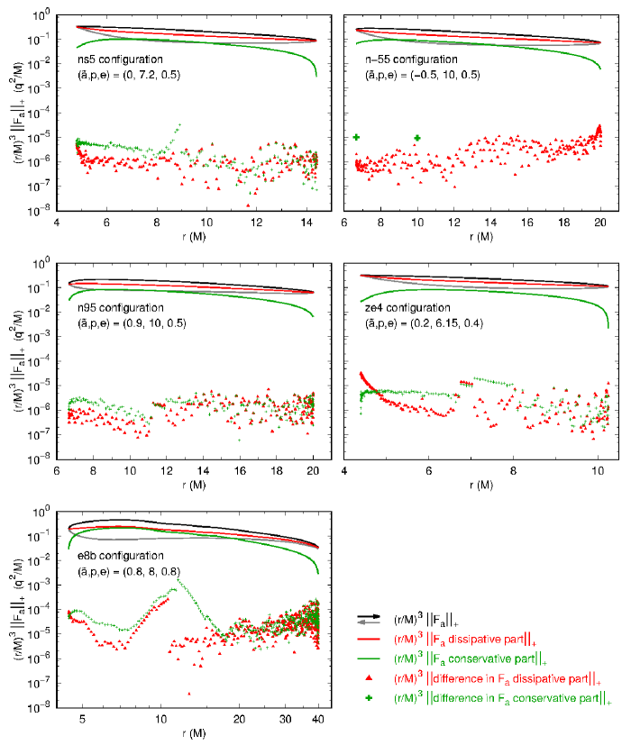
Figure 11: This figure shows the pointwise norms $\|\cdot\|_{+}$ of the differences between our computed self-force dissipative and conservative parts and values computed using Warburton and Barack’s frequency-domain code Warburton and Barack (2011). For the n-55 configuration the conservative part is compared with data for $\chi=0$ and $\chi=\pi/2$ from (Warburton and Barack, 2011, table II); all other comparisons are with unpublished results kindly provided by Warburton.

III.6 Overview of self-forces

Figures 12–22 give an overview of the computed self-forces for all our configurations. To facilitate comparison between the different configurations, these figures all use a common format (with one exception noted below):

• The top row of each figure shows auxiliary information; the lower three rows show (respectively) $F_{t}$, $F_{r}$, and $F_{\phi}$.

• In the top row, the left plot shows $r$ and $\phi$ as functions of the coordinate time $t$, while the right plot shows a plan view of the orbit, i.e., a parametric plot with $x=r(t)\cos\bigl{(}\phi(t)\bigr{)}$ and $y=r(t)\sin\bigl{(}\phi(t)\bigr{)}$.

• The coordinate-time scale always runs from $-\tfrac{1}{2}T_{r}$ to $+\tfrac{1}{2}T_{r}$, with $t=0$ corresponding to periastron. (That is, this “coordinate time” is in fact identical to the modulo time.)

• In the lower three rows of each figure, the left column of plots shows each $F_{i}$ (in units of $10^{-6}q^{2}/M$) as a function of coordinate time $t$. For the ze4, ze9, and zze9 zoom-whirl configurations, these plots also show the self-force for the circular-orbit configurations (circ-ze4, circ-ze9, and circ-zze9, respectively) with orbital radius equal to the zoom-whirl configurations’ periastron radius.

• In the lower three rows of each figure, the center and right columns of plots each show the scaled self-force $(r/M)^{3}F_{i}$ (in units of $10^{-3}q^{2}/M$). The center column of plots show $(r/M)^{3}F_{i}$ as a a function of coordinate time $t$. The right column of plots show $(r/M)^{3}F_{i}$ as a function of $r$, forming self-force “loops” plots of the type introduced by Vega et al. (2013).

• In each self-force plot (except the ze98 $r^{3}F_{i}$ plots) the total self-force is shown in black and labeled “total”, the dissipative part of the self-force is shown in red and labeled “diss”, and the conservative part of the self-force is shown in green and labeled “cons”. The dissipative and conservative parts are omitted in the ze98 $r^{3}F_{i}$ plots to reduce clutter.

• In each self-force plot the outgoing half of the orbit ($t\geq 0$) is shown in fully-saturated color (black, red, or green), while the ingoing half of the orbit ($t\leq 0$) is shown in partially-saturated color (grey, red, or green).

• In the self-force loop plots (the right column) the loops are labelled with arrows to show the particle’s direction of motion. The dissipative part of $F_{t}$, the conservative part of $F_{r}$, and the dissipative part of $F_{\phi}$ are each independent of the direction of motion. The conservative part of $F_{t}$, the dissipative part of $F_{r}$, and the conservative part of $F_{\phi}$ typically differ between ingoing (pre-periastron, $t<0$) and outgoing (post-periastron, $t>0$) motion, forming visible loops.

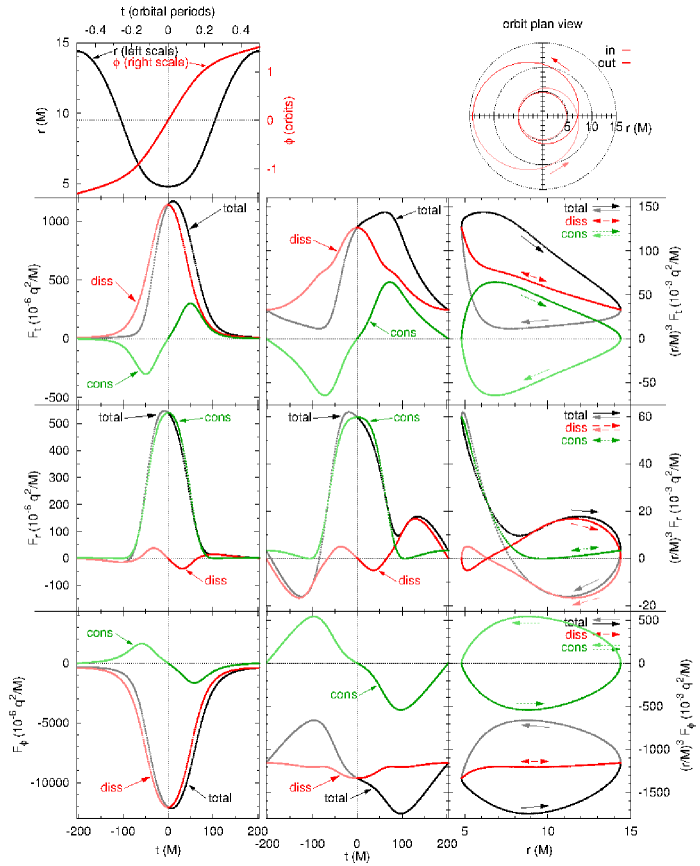
Figure 12: This figure shows the self-force for the ns5 configuration, which has $(\tilde{a},p,e)=(0,7.2,0.5)$.

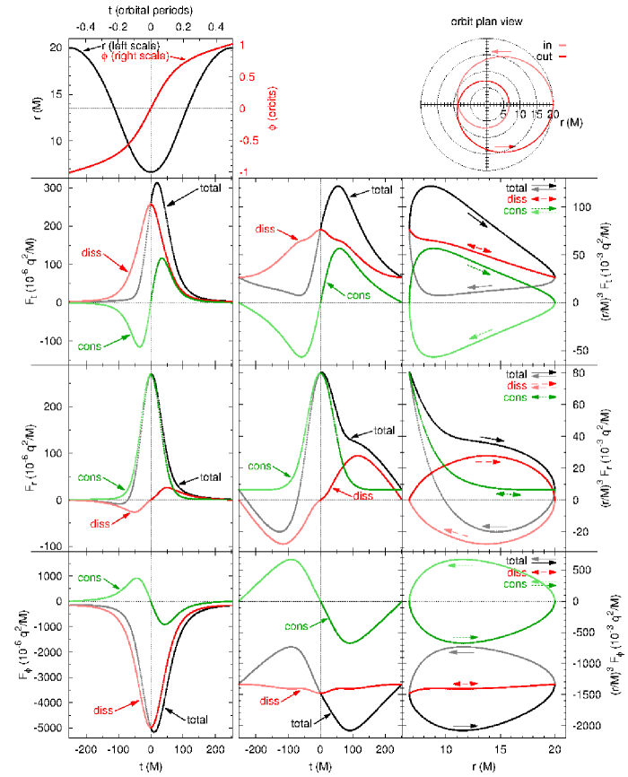
Figure 13: This figure shows the self-force for the n-55 configuration, which has $(\tilde{a},p,e)=(-0.5,10,0.5)$.

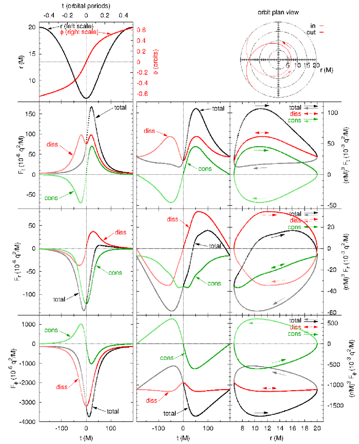
Figure 14: This figure shows the self-force for the n95 configuration, which has $(\tilde{a},p,e)=(0.9,10,0.5)$.

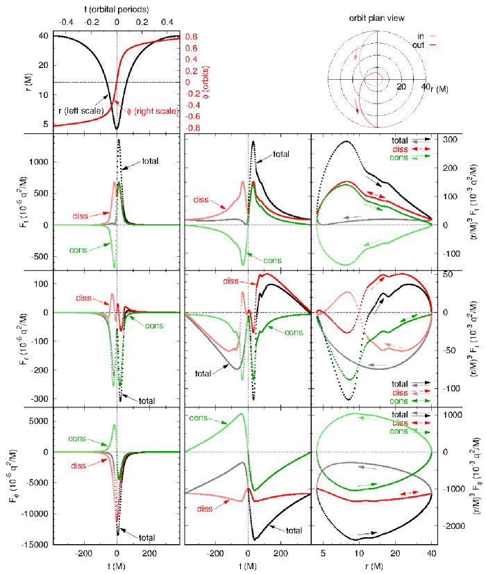
Figure 15: This figure shows the self-force for the e8 configuration, which has $(\tilde{a},p,e)=(0.6,8,0.8)$. The self-force loops (right column) are plotted using a logarithmic radial scale. Notice the wiggle in the self-force on the outgoing leg of the orbit, near $t=100\,M$ past periastron, at $r\approx 16\,M$; we discuss this in section III.9. Because the dissipative-conservative decomposition (73) and (74) is non-local, the dissipative and conservative parts of the self-force also show wiggles before periastron.

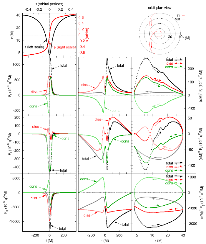
Figure 16: This figure shows the self-force for the e8b configuration, which has $(\tilde{a},p,e)=(0.8,8,0.8)$. The self-force loops (right column) are plotted using a logarithmic radial scale. Notice the wiggles in the self-force on the outgoing leg of the orbit, between $t\approx 50\,M$ and $100\,M$ past periastron, at $r\approx 15\,M$; we discuss this in section III.9. Because the dissipative-conservative decomposition (73) and (74) is non-local, the dissipative and conservative parts of the self-force also show wiggles before periastron.

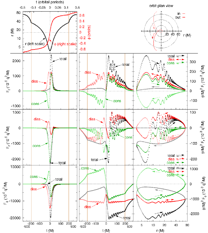
Figure 17: This figure shows the self-force for the e9 configuration, which has $(\tilde{a},p,e)=(0.99,7,0.9)$. In the time-domain plots (left and center columns) the central $|t|\leq 175\,M$ around periastron (marked by the vertical lines) is plotted at an expanded horizontal scale. The self-force loops (right column) are plotted using a logarithmic radial scale. Notice the many wiggles in the self-force on the outgoing leg of the orbit; we discuss these in section III.9. Because the dissipative-conservative decomposition (73) and (74) is non-local, the dissipative and conservative parts of the self-force also show wiggles before periastron.

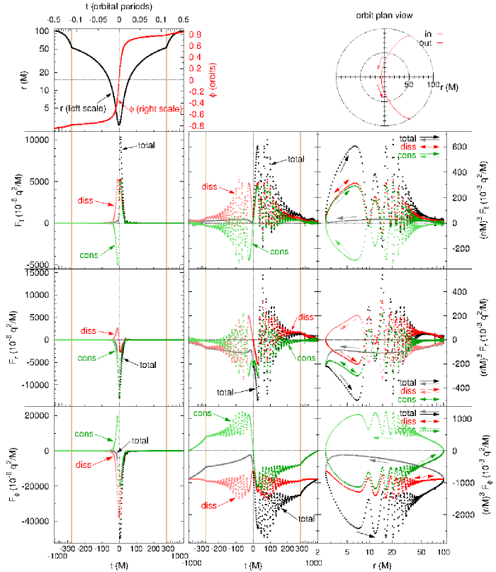
Figure 18: This figure shows the self-force for the e95 configuration, which has $(\tilde{a},p,e)=(0.99,5,0.95)$. In the time-domain plots (left and center columns) the central $|t|\leq 275\,M$ (marked by the vertical lines) is plotted at an expanded horizontal scale. The self-force loops (right column) are plotted using a logarithmic radial scale. Notice the many wiggles in the self-force on the outgoing leg of the orbit; we discuss these in section III.9. Because the dissipative-conservative decomposition (73) and (74) is non-local, the dissipative and conservative parts of the self-force also show wiggles before periastron.

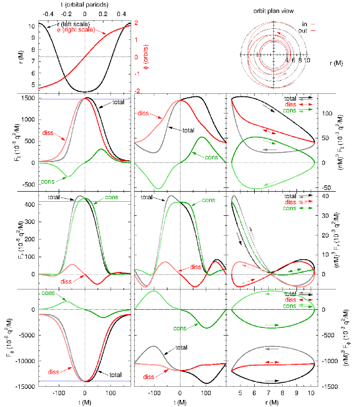
Figure 19: This figure shows the self-force for the ze4 configuration, which has $(\tilde{a},p,e)=(0.2,6.15,0.4)$. This is a mild zoom-whirl orbit; the particle completes about $2$ orbits at $r\approx 4.5\,M$ during the approximately $125\,M$ of the whirl phase. In the left column, the horizontal blue line in each self-force subplot shows the self-force for the circ-ze4 circular-orbit configuration; this configuration has the same orbital radius as the ze4 configuration’s periastron radius. The self-force near to and during the whirl phase is shown at an expanded scale in Fig 23.

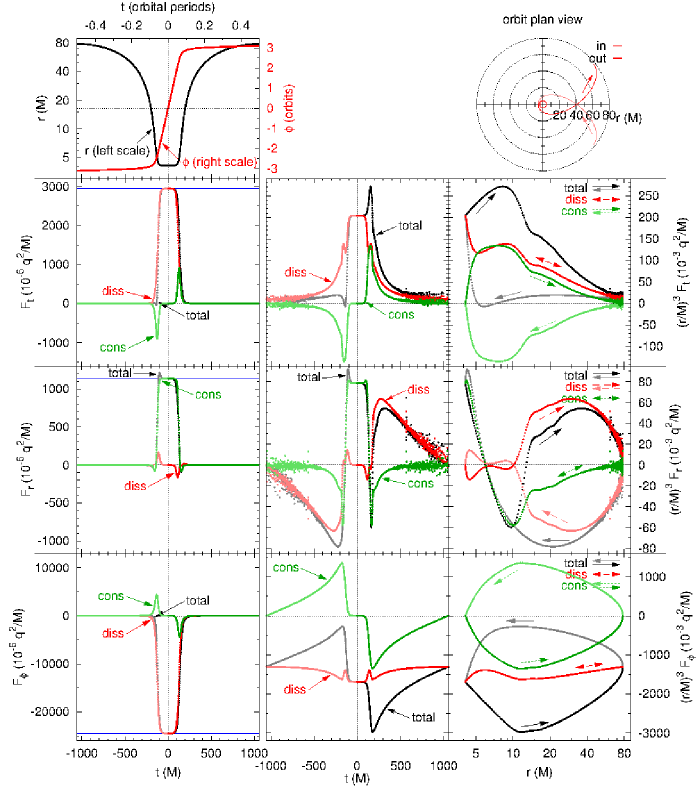
Figure 20: This figure shows the self-force for the ze9 configuration, which has $(\tilde{a},p,e)=(0.0,7.8001,0.9)$. This is a strong zoom-whirl orbit; the particle completes about $5\tfrac{1}{3}$ orbits at $r\approx 4.1\,M$ during the approximately $300\,M$ of the whirl phase. During the whirl phase the self-force is large and nearly constant; there are also “spikes” in $F_{r}$ at this phase’s entry and exit. In the left column, the horizontal blue line in each self-force subplot shows the self-force for the circ-ze9 circular-orbit configuration; this configuration has the same orbital radius as the ze9 configuration’s periastron radius. The self-force loops (right column) are plotted using a logarithmic radial scale. The self-force near to and during the whirl phase is shown at an expanded scale in Fig. 23.

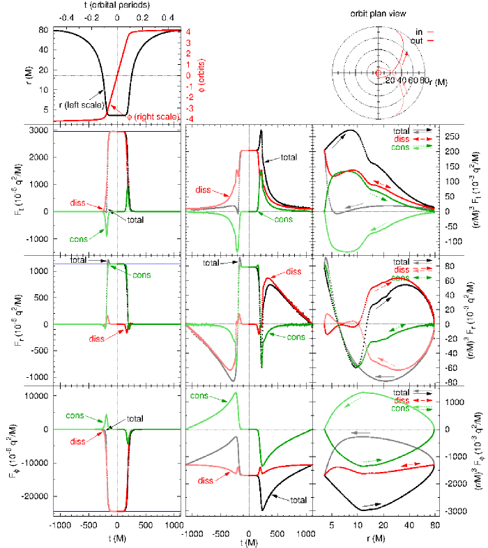
Figure 21: This figure shows the self-force for the zze9 configuration, which has $(\tilde{a},p,e)=(0.0,7.800\,001,0.9)$. This is a very strong zoom-whirl orbit; the particle completes about $7\tfrac{3}{4}$ orbits at $r\approx 4.1\,M$ during the approximately $450\,M$ of the whirl phase. During the whirl phase the self-force is large and nearly constant; there are also “spikes” in $F_{r}$ at this phase’s entry and exit. In the left column, the horizontal blue line in each self-force subplot shows the self-force for the circ-zze9 circular-orbit configuration; this configuration has the same orbital radius as the zze9 configuration’s periastron radius. The self-force loops (right column) are plotted using a logarithmic radial scale. The self-force near to and during the whirl phase is shown at an expanded scale in Fig. 23.

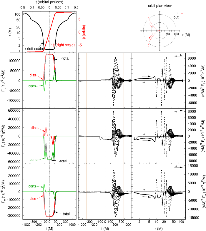
Figure 22: This figure shows the self-force for the ze98 configuration, which has $(\tilde{a},p,e)=(0.99,2.4,0.98)$. This is an extreme zoom-whirl orbit; the particle completes about $15$ orbits at $r\approx 1.2\,M$ during the approximately $220\,M$ of the whirl phase. The self-force loops (right column) are plotted using a logarithmic radial scale. During the whirl phase the self-force is very large (more than $40$ times the peak self-force of any other configuration in this study) and shows a variety of complicated phenomenology; we discuss this in section III.8. Notice the many wiggles in the self-force on the outgoing leg of the orbit; we discuss these in section III.9. The self-force near to and during the whirl phase is shown at an expanded scale in Fig. 24.

III.7 High-eccentricity orbits

Figures 15–18 show our computed self-force for the e8, e8b, e9, and e95 high-eccentricity configurations, respectively.

For these configurations the self-force is strongly localized around the periastron passage. Even though the particle spends most of its time at large radii, the $\sim r^{-3}$ far-field scaling of the self-force with radius implies that the orbital evolution will also be dominated by the periastron passage.

These configurations also show strong oscillations (“wiggles”) in the self-force shortly after the periastron passage; we discuss these in section III.9.

III.8 Zoom-whirl orbits

Figures 19–22 give an overview of our computed self-force for the ze4, ze9, zze9, and ze98 zoom-whirl configurations, respectively. Figures 23 and 24 show the self-force during the whirl phase in more detail for these configurations.

Although the self-force is strictly speaking non-local, influenced by the particle’s entire past trajectory, in practice the influence of distant times is usually small, i.e., the self-force is usually dominated by the effects of the particle’s immediate past. We thus expect that if the whirl phase of a zoom-whirl orbit is sufficiently long, the self-force should be very close to that of a circular orbit at the same radius. Figure 23 shows a numerical test of this hypothesis for the ze4, ze9, and zze9 configurations, comparing their whirl-phase self-forces to those of the corresponding circ-ze4, circ-ze9, and circ-zze9 circular-orbit configurations, respectively. For the ze4 configuration the agreement is only modest, presumably because of the relatively short whirl phase. For the ze9 and zze9 configurations the agreement is excellent.

A close examination of Figs. 20 and 21 shows small “spikes” in $F_{r}$ at the entry/exit to the ze9 and zze9 configurations’ whirl phases. These can be seen at an expanded scale in Fig. 23. At the whirl-phase entry these configurations’ $F_{r}$ first becomes slightly negative, then rises to slightly overshoot its whirl-phase value (this is the “spike” visible in Figs. 20 and 21), then decreases slightly to reach the whirl-phase value. At the whirl-phase exit $F_{r}$ decreases smoothly to a slightly negative value, then rises slightly to its post-whirl (near-zero) value. Haas (Haas, 2007, figure 17) has calculated the self-force for our ze9 configuration and finds similar overshooting behavior. Barack Barack (2016) suggests that the underlying cause of this behavior is the particle’s strong radial acceleration when entering/leaving the whirl phase, but so far as we know no quantitative explanation is known.

For the ze98 configuration (an extreme zoom-whirl orbit), Fig. 24 shows quite complicated phenomenology.

• At the entrance to the whirl phase (times $-110\,M\lesssim t\lesssim-40\,M$), $F_{r}$ shows small high-frequency oscillations superimposed on a larger lower-frequency oscillation; these oscillations last for approximately $60\,M$ (about $1/4$ of the entire whirl phase’s duration). $F_{t}$ and $F_{\phi}$ show small overshoots of their whirl-phase values, but no visible high-frequency oscillations.

• Well before the exit from the whirl phase (times $30\,M\lesssim t\lesssim 75\,M$), while the particle is still very close to a circular orbit, $F_{r}$ increases in amplitude by ${\sim}\,5\%$ (becoming more negative). Unfortunately, while our highest and 2nd-highest-resolution results agree on the overall sign of this change, they differ by roughly a factor of $2$ in its magnitude. (This is the only time at which these results differ significantly.) This suggests that higher-resolution data is needed to reliably quantify this feature.

• In this same time period (times $30\,M\lesssim t\lesssim 75\,M$) $F_{t}$ and $F_{\phi}$ both decrease in amplitude.

• Shortly before the exit from the whirl phase (times $75\,M\lesssim t\lesssim 110\,M$), when the particle is significantly departing from a near-circular orbit, all components of $F_{a}$ decrease in magnitude towards their post-whirl (small) values. None of the components shows any visible overshoot.

• All components of $F_{a}$ are significantly time-asymmetric about the periastron passage.

This phenomenology is generally consistent between the dro10-80 and dro8-64 numerical resolutions. However, this configuration is a very difficult one for our numerical evolution scheme and it remains possible that some of these features are numerical artifacts. We will need to obtain higher-resolution data to resolve this question.

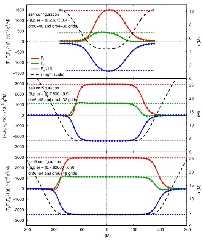
Figure 23: This figure shows the self-force during the whirl phase for the ze4, ze9, and zze9 zoom-whirl configurations. For each configuration the solid lines show the highest-resolution data, while the dots show the lower-resolution data (sampled approximately every $10\,M$); these are visually identical. The horizontal short-dashed lines show the self-force for the corresponding circular-orbit configurations (circ-ze4, circ-ze9, and circ-zze9, respectively); these have the same orbit radii as the zoom-whirl configurations’ periastrons.

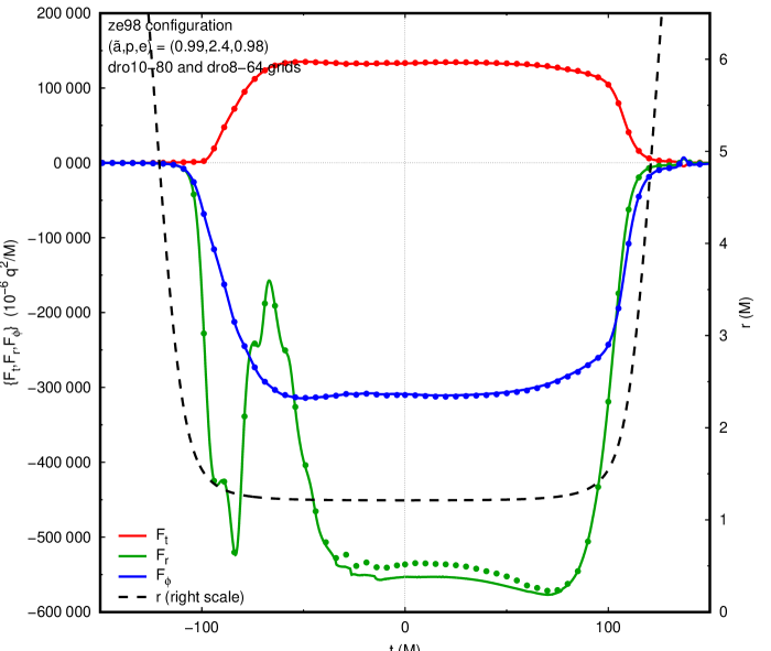
Figure 24: This figure shows the self-force during the whirl phase for the ze98 zoom-whirl configuration. The solid lines show the highest-resolution data (dro10-80 grids), while the dots show the lower-resolution data (dro8-64 grids, sampled approximately every $5\,M$); these are visually almost identical except for a $\lesssim 3.5\%$ difference in $F_{r}$ at times $-35\,M\lesssim t\lesssim 80\,M$.

III.9 Wiggles

In the configurations which combine a highly-spinning black hole and a prograde high-eccentricity orbit (the e9, e95, and ze98 configurations, shown in Figs. 17, 18, and 22 respectively), there are prominent and rapid oscillations (“wiggles”) in $r^{3}F_{a}$ shortly after periastron. These oscillations are also visible to a lesser extent in the configurations with moderate black hole spins and prograde moderate-eccentricity orbits, the e8 and e8b configurations (shown in Figs. 15 and 16 respectively). Figure 25 shows the wiggles for the e9, e95, and ze98 configurations at an expanded scale.

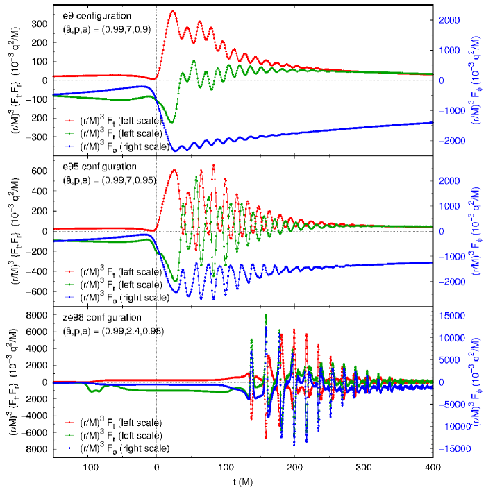
Figure 25: This figure shows the “wiggle” oscillations in $(r/M)^{3}F_{a}$ for the e9, e95, and ze98 configurations. Notice that wiggles are present only after the particle’s periastron passage ($t=0$). Notice also that for the e95 and ze98 configurations the individual wiggles are often non-sinusoidal, with shapes differing between different wiggles (this is particularly evident in the e95 $(r/M)^{3}F_{\phi}$ wiggles). The wiggles’ shapes also differ between different $F_{a}$ components.

Notice that (except for the ze98 configuration, discussed in section III.8) the self-force varies relatively smoothly prior to periastron – wiggles occur only after the particle’s periastron passage ($t=0$). This suggests that the wiggles are in some way caused by the particle’s close passage by the large black hole. We will discuss wiggles’ phenomenology and causal mechanisms in a following publication.

IV Discussion

IV.1 Overall assessment

Our computational scheme combines a number of ingredients:

• the initial formulation of the scalar-field toy model for the $\mathcal{O}(\mu)$-perturbed scalar-field equations, using a point-particle source,

• the Barack-Golbourn-Vega-Detweiler effective-source regularization,

• our specific choice for the puncture field,

• the $m$-mode Fourier decomposition, and the corresponding formulation of the puncture field and effective source in terms of elliptic integrals,

• the introduction of a worldtube, which moves in $(r,\theta)$ to follow the particle’s motion around the orbit,

• the Zenginoğlu compactification and hyperboloidal slices, and

• a finite-difference numerical evolution using Berger-Oliger mesh refinement and OpenMP-based parallelization.

The initial $\mathcal{O}(\mu)$ perturbation formulation with a point-particle source is clearly a reasonable starting point for the scalar–self-force problem. We discuss possible extensions to this in section IV.2.4.

The Barack-Golbourn-Vega-Detweiler effective-source regularization scheme works well. It involves no approximations (a solution of the regularized equation (7) is an exact solution of the $\mathcal{O}(\mu)$ field equations), the analytical computation of the singular field and effective source can be done with symbolic algebra software, and the resulting regularized equation is computationally tractable.

In this work, we use a 4th order puncture for equatorial orbits in Kerr spacetime. While higher-order, smoother punctures are available Heffernan et al. (2012, 2014), we (like other researchers Vega et al. (2009); Dolan et al. (2011); Wardell et al. (2012b); Vega et al. (2013)) find that 4th order represents a good “sweet spot” compromise between a high-order puncture — which enables high numerical accuracy and fast convergence at the cost of a having a complicated and expensive-to-evaluate source — and a low-order puncture, which is simple and fast to evaluate, but yields poor convergence and numerical accuracy. However, the computation of the effective source is still computationally expensive. Further optimization of this computation would be very useful.

The $m$-mode Fourier decomposition works very well: it provides some parallelism “for free” (each $m$-mode evolution can be performed independently), it reduces the dimensionality and hence the maximum CPU and memory usage of each individual evolution, and – perhaps most importantly – it allows different numerical techniques and/or parameters to be used for different modes’ evolutions. This last advantage may be of great importance in extending our work to the gravitational case, where Dolan and Barack Dolan and Barack (2013) found that the $m=0$ and $m=1$ modes suffer from gauge instabilities (they were able to control the $m=0$ gauge modes, but not the $m=1$ modes), while the $m\geq 2$ modes are stable.

The moving-worldtube scheme works well, allowing highly eccentric orbits to be simulated while only requiring the (expensive) effective source computation in a relatively small region of spacetime. We found the implementation of the worldtube at a finite-differencing level to be straightforward (cf. Appendix B.6) once the Boolean predicates for where to use adjusted finite differencing and where to (pre)compute the puncture field were defined correctly (cf. appendices B.7 and B.8). For orbits of low to moderate eccentricity, the alternative of using a smooth blending “window” function Vega et al. (2011, 2013) is also known to work well. However, extending this to highly eccentric orbits may require making the window function time-dependent, which would introduce additional terms into the evolution equations.

Like other researchers (e.g., Vega et al. (2011)), we find the Zenginoğlu compactification and hyperboloidal slices to work very well. They are easy to implement and provide slices which span the entire spacetime outside the event horizon, allowing stable and highly accurate horizon and $\mathcal{J}^{+}$ outgoing boundary conditions. Slices which reach $\mathcal{J}^{+}$ also allow a direct computation of the emitted radiation reaching $\mathcal{J}^{+}$, although for simplicity we have not done so here.

Our numerical evolution uses finite-differencing and Berger-Oliger mesh refinement techniques which are now standard in numerical relativity. However, there are three main complications which combine to make the use of standard adaptive-mesh-refinement frameworks such as Cactus Allen et al. (1999); Goodale et al. (2003); Cactus developers more difficult and less advantageous than would be the case in many other numerical-relativity calculations:

• Our use of a worldtube, and the associated (time-dependent) jump discontinuity in the evolved field $\varphi_{m}$, means that interpolation and restriction operators must “adjust” the field variables when crossing the worldtube boundary (cf. Appendix B.6). This means that standard mesh-refinement software requires modification to accommodate the worldtube scheme.

• The effective source is expensive to compute, but is only needed inside the worldtube, so the overall cost of integrating our equations at a single grid point is much larger inside the worldtube than outside. The default domain-decomposition parallelization heuristics used by Cactus and many other adaptive-mesh-refinement toolkits assume a roughly uniform level of computational cost per grid point across the problem domain, and thus would give relatively poor parallel performance on our computation.

• The non-smoothness of the evolved field $\varphi_{m}$ at the puncture (particle) position limits the finite-differencing order of accuracy attainable there. For our 4th order puncture, the accuracy is limited to at best $\mathcal{O}\bigl{(}(\Delta R_{*})^{2},(\Delta\theta)^{2}\bigr{)}$ because our evolution equation (25) is 2nd order in space. This reduces the benefits gained from high-order finite differencing schemes (which are now provided by many mesh-refinement software libraries).

IV.2 Possible improvements

There are a number of ways in which our results might plausibly be improved. While there is an accuracy/performance tradeoff in almost any finite difference computation, computational improvements can still usefully be categorized into those which would improve the accuracy of the self-force computation for a given finest-grid-resolution, versus those which would improve the efficiency of computing results using essentially the same numerical scheme, versus those which would improve both accuracy and efficiency.

IV.2.1 Computational improvements: accuracy

There are several ways in which our computational scheme might be improved so as to provide more accurate results for the same finest-grid-resolution.

As noted in section II.8, our interpolation scheme for computing the effective source close to the particle uses an interpolation molecule which crosses the particle position in some cases, reducing the interpolation accuracy. An improved interpolation scheme might improve the overall accuracy of the computation.

As the particle moves through the grid, the limited differentiability of $\varphi_{m}$ at the puncture effectively introduces noise into the evolution and prevents us from obtaining proper (in our case 4th order) finite differencing convergence of our results with grid resolution Choptuik (1991). One way to eliminate this noise and obtain proper finite differencing convergence would be to use finite difference operators which specifically “know” the actual functional form of $\varphi_{m}$ near the puncture. We have experimented with several finite differencing schemes of this type, but so far with only limited success. At present our code uses the “C2” scheme described in Appendix B.10. We find that this lowers the noise level in the computed self-force by roughly a factor of $3$, but our results remain quite noisy and their overall convergence order with respect to grid resolution is still much lower than we would like. Further research on finite difference operators which incorporate more of the puncture’s actual singularity structure would be useful. (We mention one possible finite differencing scheme of this type in Appendix B.10, but we were not able to obtain stable evolutions with this scheme.)

As noted in section III.3, for the e9 configuration we find poor convergence at small radii ($r\lesssim 10M$). We do not yet know the cause of this poor convergence, but fixing it would obviously be highly desirable.

Another possible route to more accurate finite differencing near the puncture might be to use many mesh-refinement levels of small grids in the puncture’s immediate neighborhood, so as to obtain very high resolutions at the puncture. Given a Berger-Oliger–style mesh-refinement infrastructure, this is not difficult. However, the interpolations of the fine-grid boundary values from the coarser grids might limit the accuracy improvement, even if buffer zones Schnetter et al. (2004) are used. Further experimentation with this type of grid structure would be useful.

Raising the order of the puncture would improve the smoothness of $\varphi_{m}$ at the puncture, improving the finite-differencing accuracy there. However, a higher-order puncture would also yield a much more complicated and expensive-to-compute effective source. Our current choice of a 4th order puncture seems to be a good compromise between smoothness and computational expense.

IV.2.2 Computational improvements: efficiency

There are a number of ways in which our computational scheme might be made more efficient.

At present our code computes the puncture field and effective source anew at each right-hand-side evaluation whose time coordinate differs from that of the previous evaluation (this happens 50% of the time for the classical 4th-order Runge-Kutta time integration scheme we currently use). For periodic orbits (including all equatorial orbits) the puncture field and effective source are the same (at a given time-past-periastron) from one orbit to the next, so a much more efficient choice would be to cache the effective source in memory, reusing cached values for all of the evolution after the first orbit. However, such a cache would use a very large amount of memory and would give no benefit for non-periodic orbits (including almost all non-equatorial orbits).

Simulations of this type are computationally expensive. Our code is currently only partially parallelized, using OpenMP to spread the computation of the singular field, effective source, and evolution-equation right-hand-side across multiple cores of a single processor. This is easy to implement and typically gives a wall-clock speedup of a factor of $12$ to $13$ using $16$ cores. Grid-based parallelism (ultimately based on message-passing) is an obvious and widely used way of achieving higher parallelism, and is now well-supported by numerical-relativity adaptive-mesh-refinement toolkits such as Cactus Allen et al. (1999); Goodale et al. (2003); Cactus developers and the Einstein toolkit Löffler et al. (2012); EinsteinToolkit . However, Cactus and many other adaptive-mesh-refinement toolkits generally assume that the cost of computing a grid point is roughly constant across the problem domain. Our worldtube scheme strongly violates that assumption: points inside the worldtube require computing the effective source and thus cost much more than points outside the worldtube. This means that without significant changes to the domain-decomposition heuristics, standard toolkits would give only limited parallel speedup for our worldtube scheme. One possible way to sidestep this issue is to use a domain decomposition for the calculation of the effective source that is independent of the normal domain decomposition of the full computational grid; such a method was used (without mesh refinement), for example, in Vega et al. (2013). Similarly, it might be that other parallelization techniques such as the task-based model used by the SpECTRE code Kidder et al. (2016) would yield better parallel speedup.

IV.2.3 Computational improvements: accuracy and efficiency

At present our computational scheme uses finite differencing with Berger-Oliger mesh refinement. A discontinuous Galerkin method Hesthaven and Warburton (2008) might give spectral (i.e., much better) accuracy/efficiency even with the limited differentiability of $\varphi_{\text{num}}$ at the particle. These methods have been used successfully in other numerical-relativity and self-force computations by a number of researchers, e.g., Field et al. (2009, 2010b); Brown et al. (2012), as well as in other areas of computational physics involving non-smooth solutions, e.g., Fan et al. (2008); Kidder et al. (2016).

Within the general framework of finite differencing and Berger-Oliger mesh refinement, there are a number of ways in which our computational scheme might be enhanced to better adjust the computations to the solution dynamics, yielding both improved accuracy (higher effective grid resolution) and efficiency (fewer high-resolution grid points “wasted” on regions of spacetime where $\varphi_{m}$ is relatively slowly-varying):

• At present our mesh-refinement scheme moves the finer grids with the worldtube but does not otherwise adapt to the solution’s dynamics. For an orbit with substantial eccentricity, the field dynamics near the particle are quite different between the particle’s periastron and apoastron. It seems likely that an adaptive mesh-refinement scheme (of the type now widely used in fully-nonlinear binary-black-hole simulations) for varying the grid structure around the orbit would substantially improve the computation’s overall accuracy/efficiency.

• At present our computational scheme keeps the worldtube size and shape fixed throughout the evolution. An adaptive scheme to adjust (optimize) these around the orbit could significantly improve the code’s accuracy and efficiency. However, unlike the case for adaptive mesh-refinement, there are no existing algorithms for making this adjustment. Further research in this area would be valuable.

• For a highly eccentric orbit, many of the higher-$m$ self-force modes are below our code’s noise level during much of the orbit. (This can be seen, for example, in Figs. 4 and 5.) The overall efficiency of the computation could be greatly improved by not computing these modes at times when they are essentially purely noise. This would require some means of estimating the time intervals in question, and changes to our initial-worldtube-setup scheme (described in section B.5) to accommodate (re)starting the computation of these modes at a time when the particle is moving much faster than near apoastron.

IV.2.4 Extensions to more general physical systems

In this work we focus on computing the instantaneous scalar self-force acting on the small body. One straightforward extension to this is to also compute the scalar field at the particle, using the method suggested in footnote 12. Another straightforward extension would be to also compute the scalar field radiated to infinity ($\mathcal{J}^{+}$). Given our use of asymptotically hyperboloidal slices which reach $\mathcal{J}^{+}$, this information is readily available. We have preliminary implementations of both of these extensions; we will discuss their results in a following publication.

Our present results are limited to (bound, geodesic) equatorial particle orbits. Apart from the computational complexity of computing the effective source (which is probably manageable with some reorganization of the Mathematica-generated C code), there appears to be no fundamental obstacle to allowing non-equatorial orbits, and this would be a very useful extension. In particular, this would allow direct exploration of transient $\theta$-$\phi$ resonances Éanna É. Flanagan and Hinderer (2012); Brink et al. (2015).

Our present results are limited to the “toy model” of a scalar-field particle. Extending these results to a point mass and its gravitational field perturbations would be very interesting but also challenging. While the basic effective-source regularization scheme is already known to be valid for the gravitational case, Dolan and Barack Dolan and Barack (2013) found that the $m=1$ evolutions suffered from linearly-growing-in-time Lorenz gauge modes which they were not able to control. Stabilizing these modes, and more generally achieving long-time-stable evolutions for all $m$, is an important area for further research.

Our present results are also limited to $\mathcal{O}(\mu)$ perturbations of the (Kerr) background spacetime. LISA could benefit from EMRI waveform templates with $\sim 10^{-8}$ or better fractional orbital-phase accuracy (Thornburg, 2011, section 4), which would require the inclusion of both $\mathcal{O}(\mu^{2})$ terms and “extended-body” effects caused by the finite size and (in general) nonzero spin of the small body (see, for example, Vines et al. (2016) and references therein).

In the longer term, it will also be essential to extend self-force calculations to include orbital evolution. This is conceptually straightforward (though computationally demanding) if the osculating-geodesic approximation is retained (as was done by Warburton et al. Warburton et al. (2012) in their pioneering calculation of gravitational inspiral in Schwarzschild spacetime over a time span of more than $75\,000$ orbits). However, going beyond the osculating-geodesic approximation is more difficult. Diener et al. Diener et al. (2012) have demonstrated that this can be done for a scalar-field particle in Schwarzschild spacetime, but they were only able to attain relatively modest accuracies and integration time spans ($\sim 20$ orbits). Extending their work to higher accuracies and longer integrations is an important area for further research.

Author Contributions

JT developed the numerical evolution and tail-fitting/mode-sum codes, performed the numerical evolutions, and did the main data analysis. BW developed the algorithms and symbolic-algebra code for computing the puncture field and effective source, and for machine-generating the C code for this computation. Both authors contributed to the preparation of this manuscript.

Appendix A $\tilde{\phi}$ derivatives

Clearly $d\tilde{\phi}=d\phi$ if $dr=0$, so for any scalar quantity $Q$ we have

$$\left.\frac{\partial Q}{\partial\phi}\right|_{r}=\left.\frac{\partial Q}{\partial\tilde{\phi}}\right|_{r},$$ (75)

i.e., (since $Q$ is arbitrary),

$$\left.\frac{\partial}{\partial\phi}\right|_{r}=\left.\frac{\partial}{\partial\tilde{\phi}}\right|_{r}.$$ (76)

To relate $\bigl{.}\partial\big{/}\partial_{r}\bigr{|}_{\phi}$ and $\bigl{.}\partial\big{/}\partial_{r}\bigr{|}_{\tilde{\phi}}$, consider two infinitesimally-separated events $X$ and $Y$, with coordinates

$$\begin{array}[]{ll@{\qquad}l@{\qquad}l}X:&r=r_{X},&\phi=\phi_{X},&\tilde{\phi}=\tilde{\phi}_{X};\\ Y:&r=r_{X}+dr,&\phi=\phi_{X}.&\end{array}$$ (77)

Since $\phi$ is the same for events $X$ and $Y$, the definition (11) of $\tilde{\phi}$ implies that $\tilde{\phi}_{Y}=\tilde{\phi}_{X}+d\tilde{\phi}$ with

$$d\tilde{\phi}=\frac{M\tilde{a}}{\Delta}dr.$$ (78)

Thus for any scalar quantity $Q$ we have (using the chain rule in $(r,\phi)$ coordinates)

$$Q_{Y}-Q_{X}=dr\cdot\left.\frac{\partial Q}{\partial r}\right|_{\phi}\qquad\text{since $d\phi=0$}.$$ (79)

Using the chain rule in $(r,\tilde{\phi})$ coordinates, we also have

$$Q_{Y}-Q_{X} =dr\cdot\left.\frac{\partial Q}{\partial r}\right|_{\tilde{\phi}}+d\tilde{\phi}\cdot\left.\frac{\partial Q}{\partial\tilde{\phi}}\right|_{r}$$ (80)

$$=dr\cdot\left.\frac{\partial Q}{\partial r}\right|_{\tilde{\phi}}+\frac{M\tilde{a}}{\Delta}dr\cdot\left.\frac{\partial Q}{\partial\tilde{\phi}}\right|_{r}\quad\text{via~{}\eqref{eqn:dphi-tilde}},$$ (81)

so that (comparing (79) and (81)) we have

$$\left.\frac{\partial Q}{\partial r}\right|_{\phi}=\left.\frac{\partial Q}{\partial r}\right|_{\tilde{\phi}}+\frac{M\tilde{a}}{\Delta}\left.\frac{\partial Q}{\partial\tilde{\phi}}\right|_{r},$$ (82)

i.e., (since $Q$ is arbitrary),

$$\left.\frac{\partial}{\partial r}\right|_{\phi}=\left.\frac{\partial}{\partial r}\right|_{\tilde{\phi}}+\frac{M\tilde{a}}{\Delta}\left.\frac{\partial}{\partial\tilde{\phi}}\right|_{r}.$$ (83)

Appendix B Details of our computational scheme

B.1 Computing $r(r_{*})$

Our computational scheme uses grids which are locally uniform in $(R_{*},\theta)$. However, the coefficients in many of our equations are given as explicit functions of $r$, so the code needs to know the $r$ coordinate of each grid point. Since $r_{*}(R)$ is given explicitly by the compactification (29) and (30), it only remains to compute $r(r_{*})$.

Given an input value $r_{*}^{\text{(input)}}$, the corresponding $r^{\text{(input)}}$ could be found by using Newton’s method to solve the equation $r_{*}(r)=r_{*}^{\text{(input)}}$ using the definition (18). However, for positions just outside the event horizon ($r_{*}\ll 0$) the near-cancellation in computing $r-r_{+}$ would make this algorithm numerically inaccurate.

Instead, we define a new radial coordinate $y$ by

$$y=\ln\left(\frac{r-r_{+}}{2M}\right)$$ (84)

so that

$$r=r_{+}+2Me^{y}.$$ (85)

The definition (18) can then be rewritten as

$$r_{*}=r+2M\frac{r_{+}}{r_{+}-r_{-}}y-2M\frac{r_{-}}{r_{+}-r_{-}}\ln\left(\frac{r_{+}-r_{-}}{2M}+e^{y}\right).$$ (86)

Given an input value $r_{*}^{\text{(input)}}$, we first find the corresponding $y^{\text{(input)}}$ by using Newton’s method to solve the equation

$$r_{*}(y)=r_{*}^{\text{(input)}}$$ (87)

for $y=y^{\text{(input)}}$, then computing $r^{\text{(input)}}$ via (85).

Newton’s method requires an initial guess $y^{(\text{initial})}$. If $r_{*}^{\text{(input)}}>r_{+}$ we guess $r^{(\text{initial})}=r_{*}$ and use (84) to compute $y^{(\text{initial})}$. Otherwise, we approximate the right hand side of (86) by its first two terms only, so that

$$y^{(\text{initial})}=\frac{r_{+}-r_{-}}{2M}\left(\frac{r_{*}^{\text{(input)}}}{r_{+}}-1\right).$$ (88)

The Newton’s-method solution is moderately expensive for a computation which (logically) is needed at each grid point: it typically requires $3$–$10$ iterations, with each iteration needing an exp() and a log() computation as well as $\sim 10$ floating-point arithmetic operations. Our code therefore precomputes and caches $r$ for each radial grid point.

B.2 Integrating Kerr geodesics

We use the Glampedakis-Kennefick formulation Glampedakis and Kennefick (2002) to integrate the Kerr geodesic equations. This parameterizes the radial motion as

$$r=\frac{pM}{1+e\cos\chi},$$ (89)

where $p$ is the dimensionless semi-latus rectum and $e$ the eccentricity. To solve for the particle position we numerically integrate the ODEs

$$\frac{dt}{d\chi} =\textsf{RHS\_t}(\chi)$$ (90a)

$$\frac{d\phi}{d\chi} =\textsf{RHS\_$\phi$}(\chi)$$ (90b)

$$\frac{d\tau}{d\chi} =\frac{(dr/d\chi)\big{/}(e\sin\chi)}{(dr/d\tau)\big{/}(e\sin\chi)}$$ (90c)

using $\chi$ is the independent variable. The right-hand-side functions RHS_t and RHS_$\phi$ are given by Glampedakis and Kennefick’s equations (17) and (16) respectively, while the right hand side of (90c) is computed using

$$\frac{dr/d\chi}{e\sin\chi} =\frac{pM}{(1+e\cos\chi)^{2}}$$ (91a)

$$\frac{dr/d\tau}{e\sin\chi} =\frac{1}{p}\sqrt{\tilde{V}_{r}(\chi)}$$ (91b)

with $\tilde{V}_{r}(\chi)$ given by Glampedakis and Kennefick’s equation (18). With this formalism the equations are non-singular at the radial turning points, and all square roots have their principal values (i.e., there are no $\pm$ sign ambiguities). However, integrating to a specified coordinate time $t$ requires either an explicit root-finding loop around the ODE integration or using an ODE integrator with built-in root-finding capabilities.

We use the ODEPACK ODE integrator Hindmarsh (1983); Radhakrishnan and Hindmarsh (1993), whose DLSODAR subroutine provides ODE integration with built-in root-finding. We typically set both the DLSODAR relative and absolute error tolerances to $100\varepsilon$, where $\varepsilon$ is the floating-point “machine epsilon”. We set the DLSODAR MXSTEP parameter (the maximum number of internal integration steps per DLSODAR call) to $10^{5}$. This allows DLSODAR to integrate a full orbit (and hence determine the orbital period) of an extreme zoom-whirl orbit like our ze98 configuration in a single call.

The ODEPACK library is written in Fortran 77, which makes its use somewhat awkward in our context. Notably, ODEPACK keeps internal state in static storage arrays and Fortran common blocks. In the context of Berger-Oliger mesh refinement it is natural to use a separate (concurrent) integration for each refinement level; in our code this requires explicitly saving and restoring the integrator state to multiplex the multiple concurrent integrations onto the single-threaded ODEPACK.

The next-generation version of ODEPACK, now known as SUNDIALS Hindmarsh et al. (2005), is written in C and (along with other algorithmic and computational improvements) directly supports multiple concurrent integrations. This should make it easier to use than the Fortran version.

B.3 Gradual turnon of the effective source

Because of the jump discontinuity in the right hand side of (25), the process of radiating away the initial junk generates high-spatial-frequency noise in $\varphi_{\text{num},m}$ in and near to the worldtube, leading to high noise levels in the computed self-force time series. Therefore, we use a gradual turn-on of the effective source, replacing (25) with

$$\Box_{m}\varphi_{\text{num},m}=\begin{cases}f(t)\,S_{\text{effective},m}&\text{inside the worldtube}\\ 0&\text{outside the worldtube}\end{cases},$$ (92)

where $f$ is a smooth function which is very small (ideally $0$) at the initial time of an evolution and increases to asymptote to $1$ at late times. We use

$$f(x)=\tfrac{1}{2}\bigl{(}1+\mathop{\text{erf}}(x)\bigr{)},$$ (93a)

where the scaled time coordinate $$x$$ is defined by

$$x(t)=A+\frac{t-t_{\text{initial}}}{B},$$ (93b)

where $$t_{\text{initial}} A=-5 B=10\,M$$ is the initial time of the time evolution, and , and .

This gives $f(t_{\text{initial}})\approx 8\,{\times}\,10^{-13}$ (sufficiently small that the noise due to $f$ being nonzero is below our code’s overall numerical noise level from other sources) and $f>0.999999$ for $t>t_{\text{initial}}+83.6\,M$ (so that our evolution equation (92) approximates (25) to within one part per million for all later times).

Using the gradual turnon of the effective source, we find that $\varphi_{\text{num},m}$ is smooth throughout a neighborhood of the worldtube (apart from being only $C^{2}$ at the particle and having the jump discontinuity (24) across the worldtube boundary) once the gradual turnon is complete and the field configuration has had time to adjust. In practice this initial startup phase has a duration of $\delta t_{\text{startup}}\sim 100\,M$ to $150\,M$.

B.4 Moving the worldtube

Figure 26 gives our worldtube-moving algorithm in detail. The algorithm is run at each base-grid time step, and has two parts: determining whether or not the worldtube should be moved at the current time and, if it should be moved, determining the new worldtube position. Table 7 gives the parameters for this algorithm (among others). In practice, we find that our computed results are quite insensitive to the precise values of these parameters (cf. Sec. III.4).

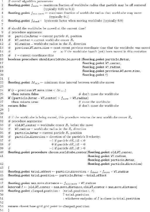
Figure 26: This figure shows our algorithm for moving the worldtube. The procedure should_worldtube_be_moved() is run at each base-grid time step to determine whether or not the worldtube should be moved at the current time, and if so, the procedure choose_worldtube_center() determines the new worldtube position.

B.5 Constraints on moving the worldtube early in the evolution

When moving the worldtube, the grid-function adjustments (26) implicitly assume that $\varphi_{\text{num}}$ has the jump discontinuity (24) across the worldtube boundary. While this is true once the field is in its equilibrium configuration, it is not true for our initial data ($\varphi_{\text{num},m}=\Pi_{\text{num},m}=0$, cf. section II.10). When the evolution begins, it takes some time (in practice $\sim 100$ to $150\,M$) for the gradual turnon of the effective source (section B.3) to be essentially complete and for the field to relax to an equilibrium configuration where the worldtube-boundary jump condition (24) is satisfied.

During this initial “startup” phase of the computation we do not know the actual jump conditions satisfied by $\varphi_{\text{num}}$, so the worldtube can not be moved. This in turn means that the initial worldtube must encompass the entire range of motion of the particle in $(R_{*},\theta)$ during the startup phase. We use the following strategy to ensure this (for a equatorial geodesic or near-geodesic particle orbit) without requiring an excessively-large worldtube:

• We first choose a particle apoastron time $t_{\text{apoastron}}$. Notice that the particle position $R_{*}=R_{*}(t)$ is locally symmetric about an (any) apoastron time.

• We then choose the startup time interval to be symmetric about $t_{\text{apoastron}}$. That is, given an estimate for the startup time interval’s duration $\delta t_{\text{startup}}$ (typically $100\,M$ to $150\,M$), we begin the numerical evolution at $t=t_{\text{initial}}=t_{\text{apoastron}}-\frac{1}{2}\delta t_{\text{startup}}$, so that the startup phase lasts until $t=t_{\text{startup}\to\text{main}}=t_{\text{apoastron}}+\frac{1}{2}\delta t_{\text{startup}}$. During the startup time interval the particle first moves outwards, then moves back inwards, reaching its initial radius again at $t_{\text{startup}\to\text{main}}$.

• We initially center the worldtube in $(R_{*},\theta)$ at (the base-grid point nearest) the average of $x^{i}_{\text{particle}}(t_{\text{initial}})$ and $x^{i}_{\text{particle}}(t_{\text{apoastron}})$, and choose the worldtube-moving parameters so that the worldtube will not be moved during the startup phase.

• At the end of the startup phase at $t_{\text{startup}\to\text{main}}$ (when the particle returns to its initial position, now moving inwards), we change the worldtube-moving parameters to values which keep the worldtube’s coordinate center within approximately half a coarse-grid spacing of the particle for the remainder of the evolution. The first worldtube move generally occurs immediately after the new parameters take effect.

B.6 Finite differencing across the worldtube boundary

We numerically implement the jump condition (24) on the worldtube boundary in the same manner as Barack and Golbourn Barack and Golbourn (2007) and Dolan and Barack Dolan and Barack (2011). That is, suppose we are finite differencing the equations at an “evaluation” grid point which is inside (outside) the worldtube, using a finite difference molecule which has a non-empty set $S$ of input grid points which are outside (inside) the worldtube. Then instead of applying the finite difference molecule to the $\varphi_{\text{num},m}$ grid function in the usual manner, we instead copy $\varphi_{\text{num},m}$ at all the molecule input points to a (molecule-sized) temporary grid function $\varphi_{\text{num},m}^{\text{temp}}$, then adjust the values of that temporary grid function to have the same inside/outside-the-worldtube semantics as the evaluation point via

$$\varphi_{\text{num},m}^{\text{temp}}\leftarrow\varphi_{\text{num},m}^{\text{temp}}\mp\varphi_{\text{puncture},m}$$ (94)

at each grid point in the set $S$, then finally apply the usual finite difference molecule to the adjusted values.

Notice that this “adjusted finite differencing” need only be used for (roughly) those grid points which are within a finite-difference molecule radius of the worldtube boundary. (We discuss the precise choice of those grid points in the following section.) Because these comprise only a tiny fraction of all grid points, the adjusted finite differencing does not itself significantly slow the code. Rather, its main computational cost is the test – at each spatial grid point at each time the evolution equations are evaluated by the time integrator – for whether or not adjusted finite differencing should be used. As discussed further in the following section, this test costs only $\sim 10$ arithmetic and logical operations, which is easily tolerable.

B.7 Computing the set of grid points where adjusted finite differencing is needed

In developing our numerical code we found that it was (is) much more difficult than might be expected to compute the precise set of grid points where adjusted finite differencing should be done. As noted in the previous section, this is approximately the set of all grid points within a finite-difference molecule radius of the worldtube boundary. However, in the presence of equatorial reflection symmetry (cf. section II.9.3) this set is not quite correct: there are certain grid points points near the intersection of the worldtube boundary with the $\theta=\pi/2$ equatorial-reflection symmetry plane which are within a finite-difference molecule radius of the worldtube boundary, but where adjusted finite differencing should (must) not be used. Figure 27 shows an example of this.

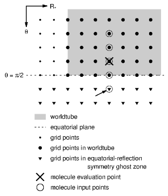
Figure 27: This figure shows an example where the naive algorithm “use adjusted finite differencing at all grid points within a finite-difference molecule radius of the worldtube boundary” would give incorrect results. The worldtube is shown by the shaded region; the worldtube boundary of interest is the “equator” $\theta=\pi/2$ (shown by the dashed line). The molecules being considered are 5-point centered molecules in the $\theta$ direction, as would be used to approximate $\partial_{\theta}$ or $\partial_{\theta\theta}$; these molecules have radius $2$ in the $\pm\theta$ directions. The molecule evaluation point shown as $\mathbf{\times}$ is only 1 grid point away from the worldtube boundary, so the naive algorithm would say that adjusted finite differencing should be used for this molecule. However, the arrowed point is actually within the equatorial-reflection symmetry ghost zone’s “reflection” of the worldtube, so in terms of the adjustment (94) this point has inside-the-worldtube semantics, and hence adjusted finite differencing should not be used for this molecule.

The technique we eventually adopted involves two parts:

1. We build up the “should this finite difference operator be adjusted via (94) at this grid point?” predicate in stages via Boolean and set operations on sets of grid points. Figure 28 shows the resulting algorithm. With this approach, the semantics of each individual function are very clear, which allowed us to develop an extensive test suite to help validate the algorithm.

2. When using equatorial-reflection symmetry, we use a numerical grid which spans only the “northern hemisphere” $0\leq\theta\leq\pi/2$ radians, but we still consider the worldtube to be the full region that it would have occupied in the absence of equatorial-reflection symmetry, i.e., (assuming an equatorial particle orbit) we take the worldtube to be symmetric about the equatorial plane.

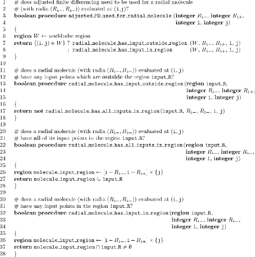
Figure 28: This figure shows our algorithm for computing the “should this finite difference operator be adjusted via (94) at this grid point?” predicate. Only the procedures for radial finite difference molecules are shown; those for angular molecules are analogous.

B.8 Computing the set of grid points where the puncture field is needed

Given that the adjustment (94) is to be applied, there remains the problem of computing $\varphi_{\text{puncture},m}$ at each finite difference molecule input point.

In our evolution scheme there are (for 5-point centered molecules) typically 9 molecule input points per evaluation point, so there is a significant performance boost from computing $\varphi_{\text{puncture},m}$ only once at each grid point where it is needed, rather than 9 times if it were (re)computed each time it is used at a molecule input point.

[Notice that – even apart from any performance cost – we can not simply compute $\varphi_{\text{puncture},m}$ at all spatial grid points (at each evaluation time), because (a) $\varphi_{\text{puncture},m}$ diverges at the particle, and (b) our series expansions for $\varphi_{\text{puncture},m}$ may be ill-behaved (e.g., they may involve division by zero) sufficiently far from the particle (outside the worldtube).]

There are two plausible ways of ensuring that $\varphi_{\text{puncture},m}$ is computed at the desired set of grid points without trying to compute it at any point where the computation would blow up:

• $\varphi_{\text{puncture},m}$ could be stored as a “smart grid function”, comprising a standard grid function of complex numbers ($\varphi_{\text{puncture},m}$ values) together with an auxiliary grid function of Boolean “valid” flags recording whether or not $\varphi_{\text{puncture},m}$ has already been computed at the corresponding grid point at the current time. On each access to the grid function, the Boolean flag would be checked, and if $\varphi_{\text{puncture},m}$ had not already been computed at that grid point at the current time, it would be computed, stored (cached) in the corresponding grid function, and the corresponding Boolean flag would be set to record that this grid-function value was now valid, so that future access could use the cached value.

• Alternatively, we could use a standard complex grid function to store $\varphi_{\text{puncture},m}$ and precompute (i.e., compute before starting to compute the adjustment (94)) $\varphi_{\text{puncture},m}$ at all the grid points where it will be needed, storing it in the grid function. (At grid points where $\varphi_{\text{puncture},m}$ will not be needed, the grid function can either be left uninitialized or be set to dummy values – these will not affect the result of any finite differencing operation.) The adjustment (94) can then use the stored $\varphi_{\text{puncture},m}$ values with no further validity checking needed.

We have chosen the second option as likely being simpler and more efficient.

The precomputation algorithm does not actually require an exact computation of the “is $\varphi_{\text{puncture},m}$ needed at this grid point?” predicate: no harm is done if we precompute $\varphi_{\text{puncture},m}$ at some points where it will not actually be used, so the predicate need only return true at a (possibly proper) superset of the actual set of grid points where $\varphi_{\text{puncture},m}$ is needed. This suggests that the naive algorithm of precomputing $\varphi_{\text{puncture},m}$ at every grid point that is within a finite-difference molecule radius of the worldtube boundary might well yield correct results.

However, for consistency and to maximize our confidence that equatorial-reflection symmetry cases like the one shown in Fig. 27 are handled correctly, we choose instead to build up the “is $\varphi_{\text{puncture},m}$ needed at this grid point?” predicate in stages using Boolean and set operations on sets of grid points, in a manner very similar to our construction of the “should adjusted finite differencing be used at this grid point?” algorithm (Fig. 28). Figure 29 shows the resulting algorithm for determining where $\varphi_{\text{puncture},m}$ is needed. Like the adjusted–finite-differencing algorithm, this algorithm has very clear semantics for each individual function, which allowed us to develop an extensive test suite to help validate the algorithm.

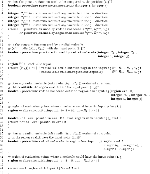
Figure 29: This figure shows our algorithm for computing the “is $\varphi_{\text{puncture},m}$ needed at this grid point?” predicate. Apart from puncture_fn_used_at_ij(), only the procedures for radial finite difference molecules are shown; those for angular molecules are analogous.

B.9 Numerical time-evolution

We numerically solve the evolution system (41) and (42) using the method of lines, with locally-uniform spatial grids in $(R_{*},\theta)$. We discretize all spatial derivatives using (5-point) 4th-order centered finite differencing, except that within a few grid points of the particle we use the “C2” finite differencing scheme described in Appendix B.10. For all results reported here, we use the classical 4th-order Runge-Kutta method for the time evolution.

We use Berger-Oliger mesh refinement (Berger (1982); Berger and Oliger (1984); Berger (1986); Berger and Colella (1989)) with a 2:1 refinement ratio, full subcycling in time, and buffer zones Schnetter et al. (2004). We use 5th-order (6-point) Lagrange polynomial interpolation in space and time for the coarse-to-fine Berger-Oliger interpolations. (This requires keeping 6 time levels for all but the finest refinement level; the latter needs only a single time level.) For the results reported here we use 4 refinement levels with the finest 3 refinement levels moved to follow the worldtube (section II.4 and table 6). In the terminology of Berger-Oliger mesh refinement our grid placement is “non-adaptive”, in that it does not depend on the values of the field variables.

While our evolution scheme is stable on moderate time scales, we find that long-time evolutions can be made much less noisy by adding 6th-order Kreiss-Oliger dissipation in the form

$$\partial_{t}\varphi_{\text{num},m} \rightarrow\partial_{t}\varphi_{\text{num},m}+\varepsilon\bigl{(}\mathsf{D}_{R_{*}}(\varphi_{\text{num},m})+\mathsf{D}_{\theta}(\varphi_{\text{num},m})\bigr{)},$$ (95a)

$$\partial_{t}\Pi_{\text{num},m} \rightarrow\partial_{t}\Pi_{\text{num},m}+\varepsilon\bigl{(}\mathsf{D}_{R_{*}}(\Pi_{\text{num},m})+\mathsf{D}_{\theta}(\Pi_{\text{num},m})\bigr{)},$$ (95b)

where

$$\bigl{(}\mathsf{D}(g)\bigr{)}_{i} =\frac{1}{64}(\Delta x)^{5}\bigl{(}D_{+}^{3}D_{-}^{3}g\bigr{)}_{i}$$

$$=\frac{1}{64\,\Delta x}(g_{i-3}-6g_{i-2}+15g_{i-1}-20g_{i}+15g_{i+1}-6g_{i+2}+g_{i+3}).$$ (96)

To obtain stable evolutions we found it crucial to add dissipation only at those grid points where the following 3 conditions are satisfied:

• The dissipation molecule does not cross the particle, i.e., the the closest grid point to the particle is not one of the points $i{-}3$ through $i{+}3$ inclusive in the expression 96.

• The dissipation molecule does not cross the worldtube boundary, i.e., it does not have input points both inside and outside the worldtube.

• The dissipation molecule does not have any input points outside the union of the nominal grid and any symmetry ghost zones. In practice this prevents dissipation from being added close to mesh-refinement boundaries or close to the horizon or $\mathcal{J}^{+}$ grid boundaries.

We use $\varepsilon=0.1$ for the evolutions reported here.

Table 9 shows the empirically determined Courant-Friedrichs-Lewy (CFL) stability limit $\nu_{\max}$ Courant et al. (1928, 1967) of our evolution scheme as a function of $m$. Our code chooses the base-grid time step $\Delta t$ by first computing $\Delta t^{(\text{preliminary})}=\kappa\nu_{\max}\,\Delta R_{*}$ (where $\kappa=0.9$ is a safety-factor parameter), then choosing $\Delta t$ to be the largest value $\leq\Delta t^{(\text{preliminary})}$ which integrally divides the output sampling time. The time steps for all refined grids are defined by the Berger-Oliger mesh refinement scheme.

It is clear from table 9 that at large $m$ our evolution scheme has a very restrictive CFL stability limit (small $\nu_{\max}$ and hence small $\Delta t$), making the evolution quite inefficient. As discussed in Appendix B.11, we have experimented with an implicit-explicit (IMEX) time evolution scheme in an attempt to alleviate the large-$m$ CFL restriction, but thus far these experiments have not yielded larger stable Courant numbers. This remains a topic for further research.

$m$	$\nu_{\max}$
0	0.630
1	0.650
2	0.590
3	0.480
4	0.390
5	0.330
6	0.283
7	0.246
8	0.217
9	0.195
10	0.176
11	0.160
12	0.147
13	0.136
14	0.127
15	0.118
16	0.111
17	0.105
18	0.099
19	0.094
20	0.089

Table 9: For each $m\in[0,20]$, this table shows the largest Courant number $\nu=\Delta t/\Delta R_{*}$ for which we obtain a stable evolution. For these stability tests we use a dissipation coefficient of $\varepsilon=0.01$ and a 2-refinement-level grid with base resolution $\Delta R_{*}=M/4$; the stability limit depends only weakly on these parameters.

B.10 Finite differencing near the particle

Because $\varphi_{m}$ is only $C^{2}$ at the particle, standard finite difference molecules do not attain their full order of accuracy near (within roughly a molecule radius of) the particle. One way to view this problem is to conceptualize a finite difference molecule as being derived by fitting a local (sliding-window) Lagrange interpolating polynomial to the operand grid function, then differentiating that interpolating polynomial. This suggests that one way to obtain more accurate finite differencing near the particle might be to use a more general interpolating function that better represents the actual behavior of $\varphi_{m}$ near the particle.

To this end, without loss of generality, we consider the finite differencing of a (real or complex) function $g$ which is defined on a suitable neighborhood of the origin on the real line, using a 1-dimensional numerical grid with grid points at integer coordinates. Without loss of generality, we assume the particle to be at the (known) position $p\in[0,\tfrac{1}{2}]$. We consider the piecewise-polynomial interpolating function

$$I(x)={} a_{0}+a_{1}(x-p)+a_{2}(x-p)^{2}$$

$$+\begin{cases}b_{3}(x-p)^{3}+b_{4}(x-p)^{4}+b_{5}(x-p)^{5}&\\ &\text{if $x\leq 0$}\\ c_{3}(x-p)^{3}+c_{4}(x-p)^{4}+c_{5}(x-p)^{5}&\\ &\text{if $x>0$}.\end{cases}$$ (97)

The 9 coefficients $\{a_{0},a_{1},a_{2},\,b_{3},b_{4},b_{5},\,c_{3},c_{4},c_{5}\}$ can be uniquely determined (as functions of the parameter $p$) by requiring $I$ to match the specified function $g$ at the 9 adjacent grid points in the range $-4\leq x\leq 4$. $I$, $dI/dx$, and $d^{2}I/dx^{2}$ can then be evaluated at any desired position to obtain finite difference approximations to $g$, $dg/dx$, and $d^{2}g/dx^{2}$ respectively. Using a symbolic algebra system, these finite-difference operators can be written as linear combinations of the values of $g$ at the grid points, with coefficients depending only on $p$ and the evaluation position.

Figure 30 shows how we use these “C2” finite-difference operators at various grid points near the particle. In the present work the particle is always in the background Kerr spacetime’s equatorial plane, and we always place a $\theta=\text{constant}$ row of grid points on the equatorial plane. Considering the numerical grid in 2 dimensions $(R_{*},\theta)$, with corresponding integer grid coordinates $(\textsf{i},\textsf{j})$, suppose that the closest grid point to the particle is at $(\textsf{i}_{\text{particle}},\textsf{j}_{\text{equator}})$. Then we use the C2 scheme for $\partial_{R_{*}}$ and $\partial_{R_{*}R_{*}}$ derivatives evaluated at grid points on the equator (i.e., for grid points with $\textsf{j}=\textsf{j}_{\text{equator}}$) and i near $\textsf{i}_{\text{particle}}$, in the manner shown in the figure. We also use this scheme in the j direction for $\partial_{\theta}$ and $\partial_{\theta\theta}$ derivatives evaluated at grid points with $\textsf{i}=\textsf{i}_{\text{particle}}$ and j near the equator. We use standard (5-point) centered 4th-order molecules at all other grid points.

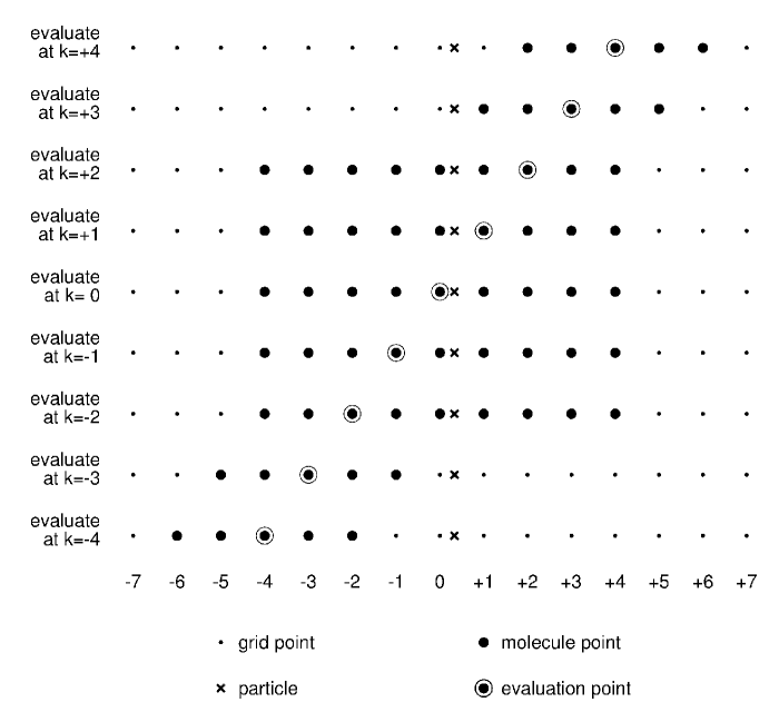
Figure 30: This figure shows our “C2” spatial finite differencing scheme for use near the particle. Each row of the diagram shows the finite difference molecule used for a different evaluation point. “k” refers to the integer grid coordinate in the $x$ direction, with the origin set so that $\textsf{k}\,{=}\,0$ is the grid point closest to the particle. We use molecules based on the piecewise-polynomial interpolating function (97) for evaluations points $-2\leq\textsf{k}\leq+2$ and standard (5-point) centered 4th-order molecules at all other evaluation points.

As discussed in section II.11, we also use the interpolating function $I$ directly in computing the self-force.

Overall, we find that switching from using 4th-order centered spatial finite differencing everywhere to using the C2 finite-difference operators near the particle reduces the noise level in the computed self-force by about a factor of $2$ to $3$.

We also experimented with a more general interpolating function

$$I(x)=a_{0}+a_{1}(x-p)+a_{2}(x-p)^{2}+\begin{cases}\phantom{+}b_{3}(x-p)^{3}+b_{3\ell}(x-p)^{3}\log\bigl{(}K(x-p)^{2}\bigr{)}&\\ +b_{4}(x-p)^{4}+b_{4\ell}(x-p)^{4}\log\bigl{(}K(x-p)^{2}\bigr{)}&\\ +b_{5}(x-p)^{5}+b_{5\ell}(x-p)^{5}\log\bigl{(}K(x-p)^{2}\bigr{)}&\text{if $x\leq 0$}\\[4.30554pt] \phantom{+}c_{3}(x-p)^{3}+c_{3\ell}(x-p)^{3}\log\bigl{(}K(x-p)^{2}\bigr{)}&\\ +c_{4}(x-p)^{4}+c_{4\ell}(x-p)^{4}\log\bigl{(}K(x-p)^{2}\bigr{)}&\\ +c_{5}(x-p)^{5}+c_{5\ell}(x-p)^{5}\log\bigl{(}K(x-p)^{2}\bigr{)}&\text{if $x>0$,}\end{cases}$$ (98)

where $K$ is a scaling constant and the 15 coefficients $\{a_{i},b_{i},b_{i\ell},c_{i},c_{i\ell}\}$ are determined by solving a system of 15 linear equations using the values of $g$ at 15 adjacent grid points. (A purely symbolic solution to this linear system proved impractical, but it is easy to solve numerically. This needs to be done once for each choice of the grid spacing and $K$.) However, we were not able to obtain stable evolutions with this scheme.

B.11 Implicit-explicit (IMEX) evolution schemes

As discussed in Appendix B.9, when using an explicit (Runge-Kutta) time evolution scheme we find that the CFL stability limit Courant et al. (1928, 1967) is very restrictive for large $m$, with the largest stable Courant number being approximately proportional to $1/m$. Examination of the derivative structure of our evolution system, together with an eigenvalue analysis kindly performed by I. Hinder, suggests that $m^{2}$ coefficient in the $\varphi$ term in the scalar wave operator (22) may be a major contributor to the large-$m$ time-step restriction.

We thus consider the use of an implicit time evolution scheme. More precisely, we consider the the use of an implicit-explicit (IMEX) time evolution scheme. There is a large literature on these schemes; see, for example, Ascher et al. (1995, 1997); Pareschi and Russo (2000, 2005); Boscarino (2007, 2009); Boscarino and Russo (2009). The basic concept of an IMEX scheme is to partition the right-hand-side function into explicit and implicit parts,

$$\dot{\mathsf{u}}=\mathsf{F}(\mathsf{u},t)+\mathsf{G}(\mathsf{u},t),$$ (99)

where $\mathsf{u}$ is the state vector, then treat $\mathsf{F}$ explicitly and $\mathsf{G}$ implicitly. For our application, we will place all the spatial derivatives into the explicit term, thus avoiding having to solve an elliptic system at each time step.

We have chosen the scheme proposed by Boscarino Boscarino (2009) (in particular, his BHR(5,5,3) scheme, variant 2) as being efficient, relatively easy to implement, and having good accuracy (3rd order overall) without the “order reduction” problems of many other schemes.

We write a generic implicit-explicit Runge-Kutta scheme for the ODE (99) as

$$\mathsf{u}^{(n+1)}=\mathsf{u}^{(n)}+h\sum_{i=1}^{s}b_{i}\mathsf{k}_{i}+h\sum_{i=1}^{\tilde{s}}\tilde{b}_{i}\tilde{\mathsf{k}}_{i},$$ (101)

where $h$ is the time step, superscripts ⁽ⁿ⁾ and ⁽ⁿ⁺¹⁾ refer to time levels, subscripts refer to Runge-Kutta stages numbered $1,\dots,s$, and the Runge-Kutta stages are given by

$$\mathsf{k}_{i} =F(\mathsf{u}_{i},t^{(n)}+hc_{i}),$$ (102a)

$$\tilde{\mathsf{k}}_{i} =G(\mathsf{u}_{i},t^{(n)}+hc_{i}),$$ (102b)

$$\mathsf{u}_{i} =\mathsf{u}^{(n)}+h\sum_{j<i}d_{ij}\mathsf{k}_{j}+h\sum_{j\leq i}\tilde{d}_{ij}\tilde{\mathsf{k}}_{j},$$ (102c)

with the coefficients $\{b_{i}\}$, $\{\tilde{b}_{i}\}$, $\{c_{i}\}$, $\{d_{ij}\}$, and $\{\tilde{d}_{ij}\}$

For example (eliding the evaluation times for clarity), the first few stages are

$$\mathsf{u}_{1} =\mathsf{u}^{(n)}+h\tilde{d}_{11}\mathsf{G}(\mathsf{u}_{1}),$$ (103a)

$$\mathsf{u}_{2} =\mathsf{u}^{(n)}+hd_{21}\mathsf{F}(\mathsf{u}_{1})+h\tilde{d}_{21}\mathsf{G}(\mathsf{u}_{1})+h\tilde{d}_{22}\mathsf{G}(\mathsf{u}_{2}),$$ (103b)

$$\mathsf{u}_{3} =\mathsf{u}^{(n)}+hd_{31}\mathsf{F}(\mathsf{u}_{1})+hd_{32}\mathsf{F}(\mathsf{u}_{2})$$

$$\qquad+h\tilde{d}_{31}\mathsf{G}(\mathsf{u}_{1})+h\tilde{d}_{32}\mathsf{G}(\mathsf{u}_{2})+h\tilde{d}_{33}\mathsf{G}(\mathsf{u}_{3}).$$ (103c)

To solve the implicit equations (102), we observe that our state vector $\mathsf{u}$ is of the form

$$\mathsf{u}=\left(\begin{array}[]{c}\varphi\\ \Pi\end{array}\right),$$ (104)

so we can write

$$\mathsf{F}\left(\begin{array}[]{c}\varphi\\ \Pi\end{array}\right)=\left(\begin{array}[]{c}y(\varphi,\Pi)\\ z(\varphi,\Pi)\end{array}\right)$$ (105)

and

$$\mathsf{G}\left(\begin{array}[]{c}\varphi\\ \Pi\end{array}\right)=\left(\begin{array}[]{c}0\\ \tilde{z}(\varphi,\Pi)\end{array}\right)=\left(\begin{array}[]{c}0\\ \alpha\varphi+\beta\Pi\end{array}\right)$$ (106)

with known coefficients $\alpha$ and $\beta$. (This use of $\alpha$ is unrelated to its use as a tail-series exponent in section II.12.)

The 2-component $\mathsf{F}$ function (105) includes all the main evolution equations (41), (42), and (95), as well as all spatial boundary conditions. Evaluating $F$ requires computing (or retrieving from a cache) the 2-D puncture field and effective source.

We have considered a number of possible choices for precisely which terms from the main evolution equation (42) should be treated implicitly (i.e., put into $G$). Conceptually, we have $\alpha=\alpha_{1}+\alpha_{2}+\alpha_{3}$, where

$$\alpha_{1} =\text{$0$ or $\displaystyle-\frac{2\Delta}{r(r^{2}+M^{2}\tilde{a}^{2})^{2}}\left(M-\frac{M^{2}\tilde{a}^{2}}{r}\right)$},$$ (107a)

$$\alpha_{2} =\text{$0$ or $\displaystyle-\frac{m^{2}\Delta}{(r^{2}+M^{2}\tilde{a}^{2})^{2}\sin^{2}\theta}$},$$ (107b)

$$\alpha_{3} =\text{$0$ or $\displaystyle-i\frac{2mM\tilde{a}\Delta}{r(r^{2}+M^{2}\tilde{a}^{2})^{2}}$},$$ (107c)

and

$$\beta =\text{$0$ or $\displaystyle-i\frac{4mM^{2}\tilde{a}r}{(r^{2}+M^{2}\tilde{a}^{2})^{2}}$}$$ (107d)

modified by the compactification transformation (37), together with the spatial boundary conditions. This gives 16 possible variant schemes, depending on which subset of $\{\alpha_{1},\alpha_{2},\alpha_{3},\beta\}$ is nonzero (treated implicitly). For each of these variants,

• $\mathsf{G}$ is linear in $\varphi$ and $\Pi$ at each grid point,

• $\mathsf{G}$ may be evaluated independently at each grid point, and

• this evaluation does not require computing the 2-D puncture field or effective source.

Together, these properties make the scheme efficient and relatively easy to implement.

Substituting the 2-component $\mathsf{u}$, $\mathsf{F}$, and $\mathsf{G}$ functions (104), (105), and (106) into the implicit Runge-Kutta equations (102), we have

$$\mathsf{u}_{i}=\left(\begin{array}[]{c}\varphi_{i}\\ \Pi_{i}\end{array}\right) =\left(\begin{array}[]{c}\varphi^{(n)}\\ \Pi^{(n)}\end{array}\right)+h\sum_{j<i}d_{ij}\left(\begin{array}[]{c}y_{j}\\ z_{j}\end{array}\right)$$ (114)

$$+h\sum_{j<i}\tilde{d}_{ij}\left(\begin{array}[]{c}0\\ \tilde{z}_{j}\end{array}\right)+h\tilde{d}_{ii}\left(\begin{array}[]{c}0\\ \alpha\varphi_{i}+\beta\Pi_{i}\end{array}\right).$$ (119)

We solve this equation at each Runge-Kutta stage by first computing

$$\varphi_{i}=\varphi^{(n)}+h\sum_{j<i}d_{ij}y_{j}$$ (120a)

and then computing

$$\Pi_{i}=\frac{\displaystyle\Pi^{(n)}+h\sum_{j<i}d_{ij}z_{j}+h\sum_{j<i}\tilde{d}_{ij}\tilde{z}_{j}+h\tilde{d}_{ii}\alpha\varphi_{i}}{1-h\tilde{d}_{ii}\beta}.$$ (120b)

We have implemented these 16 variant schemes, but unfortunately we find that all of them have CFL stability limits which are (to within the $\sim 1\%$ accuracy of our trial-and-error estimation of the stability limit on test problems) identical to those of the classical RK4 scheme (table 9). Since the RK4 scheme is simpler and offers a factor-of-two overall speedup by caching and reusing the effective source at repated evaluation times, we use it for all the computations presented in this paper. We hope to further investigate different partitionings of the right-hand-side function between $\mathsf{F}$ and $\mathsf{G}$ in the future in the hopes of alleviating the large-$m$ time-step restriction.

References

- Gair et al. (2004) J. R. Gair, L. Barack, T. Creighton, C. Cutler, S. L. Larson, E. S. Phinney, and M. Vallisneri, Class. Quant. Grav. 21, S1595 (2004), gr-qc/0405137 .
- Barack and Cutler (2004) L. Barack and C. Cutler, Phys. Rev. D 69, 082005 (2004), gr-qc/0310125 .
- Amaro-Seoane et al. (2007) P. Amaro-Seoane, J. R. Gair, M. Freitag, M. C. Miller, I. Mandel, C. J. Cutler, and S. Babak, Class. Quant. Grav. 24, R113 (2007), astro-ph/0703495 .
- Gair (2009) J. R. Gair, Class. Quant. Grav. 26, 094034 (2009), arXiv:0811.0188 .
- Damour (1987) T. Damour, in Three Hundred Years of Gravitation, edited by S. W. Hawking and W. Israel (Cambridge University Press, Cambridge, England, 1987) Chap. 6, pp. 128–198.
- Blanchet (2014) L. Blanchet, Living Reviews in Relativity 17, 2 (2014).
- Futamase and Itoh (2007) T. Futamase and Y. Itoh, Living Reviews in Relativity 10, 2 (2007).
- Blanchet (2011) L. Blanchet, in Mass and Motion in General Relativity, Fundamental Theories of Physics, Vol. 162, edited by L. Blanchet, A. Spallicci, and B. F. Whiting (Springer-Verlag, Berlin, 2011) pp. 125–166, arXiv:0907.3596 .
- Schäfer (2011) G. Schäfer, in Mass and Motion in General Relativity, Fundamental Theories of Physics, Vol. 162, edited by L. Blanchet, A. Spallicci, and B. F. Whiting (Springer-Verlag, Berlin, 2011) pp. 167–210, arXiv:0910.2857 .
- Pretorius (2007) F. Pretorius, in Relativistic Objects in Compact Binaries: From Birth to Coalescence, edited by M. Colpi (Springer-Verlag, 2007) arXiv:0710.1338 .
- Hannam et al. (2009) M. Hannam, S. Husa, J. G. Baker, M. Boyle, B. Brügmann, T. Chu, N. Dorband, F. Herrmann, I. Hinder, B. J. Kelly, L. E. Kidder, P. Laguna, K. D. Matthews, J. R. van Meter, H. P. Pfeiffer, D. Pollney, C. Reisswig, M. A. Scheel, and D. Shoemaker, Phys. Rev. D 79, 084025 (2009), arXiv:0901.2437 .
- Hannam (2009) M. Hannam, Class. Quant. Grav. 26, 114001 (2009), arXiv:0901.2931 .
- Hannam and Hawke (2011) M. Hannam and I. Hawke, General Relativity and Gravitation 43, 465 (2011), arXiv:0908.3139 .
- Campanelli et al. (2010) M. Campanelli, C. O. Lousto, B. C. Mundim, H. Nakano, Y. Zlochower, and H.-P. Bischof, Class. Quant. Grav. 27, 084034 (2010), arXiv:1001.3834 .
- Bishop et al. (2003) N. T. Bishop, R. Gómez, S. Husa, L. Lehner, and J. Winicour, Phys. Rev. D 68, 084015 (2003), gr-qc/0301060 .
- Bishop et al. (2005) N. T. Bishop, R. Gómez, L. Lehner, M. Maharaj, and J. Winicour, Phys. Rev. D 72, 024002 (2005), gr-qc/0412080 .
- Sopuerta et al. (2006) C. F. Sopuerta, P. Sun, P. Laguna, and J. Xu, Class. Quant. Grav. 23, 251 (2006), gr-qc/0507112 .
- Sopuerta and Laguna (2006) C. F. Sopuerta and P. Laguna, Phys. Rev. D 73, 044028 (2006), gr-qc/0512028 .
- Lousto et al. (2010) C. O. Lousto, H. Nakano, Y. Zlochower, and M. Campanelli, Phys. Rev. Lett. 104, 211101 (2010), arXiv:1001.2316 .
- Lousto and Zlochower (2011) C. O. Lousto and Y. Zlochower, Phys. Rev. Lett. 106, 041101 (2011), arXiv:1009.0292 .
- Poisson et al. (2011) E. Poisson, A. Pound, and I. Vega, Living Reviews in Relativity 14, 7 (2011).
- Geroch and Traschen (1987) R. Geroch and J. Traschen, Phys. Rev. D 36, 1017 (1987).
- Steinbauer and Vickers (2006) R. Steinbauer and J. A. Vickers, Class. Quant. Grav. 23, R91 (2006), gr-qc/0603078v2 .
- Mino et al. (1997) Y. Mino, M. Sasaki, and T. Tanaka, Phys. Rev. D 55, 3457 (1997), gr-qc/9606018 .
- Quinn and Wald (1997) T. C. Quinn and R. M. Wald, Phys. Rev. D 56, 3381 (1997), gr-qc/9610053 .
- Detweiler (2001) S. Detweiler, Phys. Rev. Lett. 86, 1931 (2001), gr-qc/0011039 .
- Gralla and Wald (2008) S. E. Gralla and R. M. Wald, Class. Quant. Grav. 25, 205009 (2008), arXiv:0806.3293 .
- Gralla et al. (2009) S. E. Gralla, A. I. Harte, and R. M. Wald, Phys. Rev. D 80, 024031 (2009), arXiv:0905.2391 .
- Detweiler (2005) S. Detweiler, Class. Quant. Grav. 22, S681 (2005), gr-qc/0501004 .
- Barack (2009) L. Barack, Class. Quant. Grav. 26, 213001 (2009), arXiv:0908.1664 .
- Barack (2011) L. Barack, in Mass and Motion in General Relativity, Fundamental Theories of Physics, Vol. 162, edited by L. Blanchet, A. Spallicci, and B. F. Whiting (Springer-Verlag, Berlin, 2011) pp. 327–366.
- Burko (2011) L. M. Burko, in Mass and Motion in General Relativity, Fundamental Theories of Physics, Vol. 162, edited by L. Blanchet, A. Spallicci, and B. F. Whiting (Springer-Verlag, Berlin, 2011) pp. 395–414.
- Detweiler (2011) S. Detweiler, in Mass and Motion in General Relativity, Fundamental Theories of Physics, Vol. 162, edited by L. Blanchet, A. Spallicci, and B. F. Whiting (Springer-Verlag, Berlin, 2011) pp. 271–307, arXiv:0908.4363 .
- Poisson (2011) E. Poisson, in Mass and Motion in General Relativity, Fundamental Theories of Physics, Vol. 162, edited by L. Blanchet, A. Spallicci, and B. F. Whiting (Springer-Verlag, Berlin, 2011) pp. 309–325, arXiv:0909.2994 .
- Wald (2011) R. M. Wald, in Mass and Motion in General Relativity, Fundamental Theories of Physics, Vol. 162, edited by L. Blanchet, A. Spallicci, and B. F. Whiting (Springer-Verlag, Berlin, 2011) pp. 253–262, arXiv:0907.0412 .
- Sago et al. (2008) N. Sago, L. Barack, and S. Detweiler, Phys. Rev. D 78, 124024 (2008), arXiv:0810.2530 .
- Barack and Ori (2000) L. Barack and A. Ori, Phys. Rev. D 61, 061502(R) (2000), gr-qc/9912010 .
- Barack (2000) L. Barack, Phys. Rev. D 62, 084027 (2000), gr-qc/0005042 .
- Barack et al. (2002) L. Barack, Y. Mino, H. Nakano, A. Ori, and M. Sasaki, Phys. Rev. Lett. 88, 091101 (2002), gr-qc/0111001 .
- Barack and Ori (2002) L. Barack and A. Ori, Phys. Rev. D 66, 084022 (2002), gr-qc/0204093 .
- Barack and Ori (2003) L. Barack and A. Ori, Phys. Rev. D 67, 024029 (2003), gr-qc/0209072 .
- Detweiler and Whiting (2003) S. Detweiler and B. F. Whiting, Phys. Rev. D 67, 024025 (2003), gr-qc/0202086 .
- Detweiler et al. (2003) S. Detweiler, E. Messaritaki, and B. F. Whiting, Phys. Rev. D 67, 104016 (2003), gr-qc/0205079 .
- Haas and Poisson (2006) R. Haas and E. Poisson, Phys. Rev. D 74, 044009 (2006), gr-qc/0605077 .
- Anderson and Wiseman (2005) W. G. Anderson and A. G. Wiseman, Class. Quant. Grav. 22, S783 (2005), arXiv:gr-qc/0506136 [gr-qc] .
- Casals et al. (2009) M. Casals, S. R. Dolan, A. C. Ottewill, and B. Wardell, Phys. Rev. D79, 124043 (2009), arXiv:0903.0395 [gr-qc] .
- Casals et al. (2013) M. Casals, S. Dolan, A. C. Ottewill, and B. Wardell, Phys. Rev. D88, 044022 (2013), arXiv:1306.0884 [gr-qc] .
- Wardell et al. (2014) B. Wardell, C. R. Galley, A. Zenginoğlu, M. Casals, S. R. Dolan, and A. C. Ottewill, Phys. Rev. D 89, 084021 (2014), http://arxiv.org/abs/1401.1506 .
- Barack and Golbourn (2007) L. Barack and D. A. Golbourn, Phys. Rev. D 76, 044020 (2007), arXiv:0705.3620 .
- Vega and Detweiler (2008) I. Vega and S. Detweiler, Phys. Rev. D 77, 084008 (2008), arXiv:0712.4405 .
- Wardell (2015) B. Wardell, in Equations of Motion in Relativistic Gravity, Fundamental Theories of Physics, Vol. 179, edited by D. Puetzfeld, C. Lämmerzahl, and B. Schutz (Springer International Publishing, 2015) pp. 487–522, arXiv:1501.07322 .
- Warburton and Barack (2011) N. Warburton and L. Barack, Phys. Rev. D 83, 124038 (2011), arXiv:1103.0287 .
- Wardell et al. (2012a) B. Wardell, I. Vega, J. Thornburg, and P. Diener, Phys.Rev. D85, 104044 (2012a), arXiv:1112.6355 [gr-qc] .
- Blanchet et al. (2010) L. Blanchet, S. Detweiler, A. Le Tiec, and B. F. Whiting, Phys. Rev. D 81, 064004 (2010), arXiv:0910.0207 .
- Shah et al. (2011) A. G. Shah, T. S. Keidl, J. L. F. D.-H. Kim, and L. R. Price, Phys. Rev. D 83, 064018 (2011), arXiv:1009.4876 .
- Heffernan et al. (2012) A. Heffernan, A. Ottewill, and B. Wardell, Phys.Rev. D86, 104023 (2012), arXiv:1204.0794 [gr-qc] .
- Johnson-McDaniel et al. (2015) N. K. Johnson-McDaniel, A. G. Shah, and B. F. Whiting, Phys. Rev. D 92, 044007 (2015), arXiv:1503.02638 .
- Glampedakis and Kennefick (2002) K. Glampedakis and D. Kennefick, Phys. Rev. D 66, 044002 (2002).
- Barack and Lousto (2005) L. Barack and C. O. Lousto, Phys. Rev. D 72, 104026 (2005), gr-qc/0510019 .
- Barack et al. (2008) L. Barack, A. Ori, and N. Sago, Phys. Rev. D 78, 084021 (2008), arXiv:0808.2315 .
- Barton et al. (2008) J. L. Barton, D. J. Lazar, D. J. Kennefick, G. Khanna, and L. M. Burko, Phys. Rev. D 78, 064042 (2008), arXiv:0804.1075 .
- Haas (2007) R. Haas, Phys. Rev. D 75, 124011 (2007), arXiv:0704.0797 .
- Barack and Sago (2010) L. Barack and N. Sago, Phys. Rev. D 81, 084021 (2010), arXiv:1002.2386 .
- Hopman and Alexander (2005) C. Hopman and T. Alexander, The Astrophysical Journal 629, 362 (2005), astro-ph/0503672 .
- Wald (1984) R. M. Wald, General relativity (The University of Chicago Press, Chicago, 1984).
- Brill et al. (1972) D. R. Brill, P. L. Chrzanowski, C. M. Pereira, E. D. Fackerell, and J. R. Ipser, Phys. Rev. D 5, 1913 (1972).
- Teukolsky (1973) S. A. Teukolsky, Astrophys. J. 185, 635 (1973).
- Vega et al. (2011) I. Vega, B. Wardell, and P. Diener, Class. Quant. Grav. 28, 134010 (2011), arXiv:1101.2925 .
- Vega et al. (2009) I. Vega, P. Diener, W. Tichy, and S. Detweiler, Phys. Rev. D 80, 084021 (2009), arXiv:0908.2138 .
- Diener et al. (2012) P. Diener, I. Vega, B. Wardell, and S. Detweiler, Phys. Rev. Lett. 108, 191102 (2012), arXiv:1112.4821 .
- Vega et al. (2013) I. Vega, B. Wardell, P. Diener, S. Cupp, and R. Haas, Phys. Rev. D 88, 084021 (2013), arXiv:1307.3476 .
- Barack et al. (2007) L. Barack, D. A. Golbourn, and N. Sago, Phys. Rev. D 76, 124036 (2007), arXiv:0709.4588 .
- Dolan and Barack (2011) S. R. Dolan and L. Barack, Phys. Rev. D 83, 024019 (2011), arXiv:1010.5255 .
- Dolan et al. (2011) S. R. Dolan, B. Wardell, and L. Barack, Phys. Rev. D 84, 084001 (2011), arXiv:1010.5255 .
- Dolan and Barack (2013) S. R. Dolan and L. Barack, Phys. Rev. D 87, 084066 (2013), arXiv:1211.4586 .
- Krivan et al. (1996) W. Krivan, P. Laguna, and P. Papadopoulos, Phys. Rev. D 54, 4728 (1996), gr-qc/9606003 .
- Sundararajan et al. (2007) P. A. Sundararajan, G. Khanna, and S. A. Hughes, Phys. Rev. D 76, 104005 (2007), gr-qc/0703028 .
- Zenginoğlu (2008a) A. Zenginoğlu, Class. Quant. Grav. 25, 145002 (2008a), arXiv:0712.4333 .
- Zenginoğlu (2008b) A. Zenginoğlu, Class. Quant. Grav. 25, 195025 (2008b), arXiv:0808.0810 .
- Zenginoğlu (2011) A. Zenginoğlu, J. Comp. Phys. 230, 2286 (2011), arXiv:1008.3809 .
- Zenginoğlu and Khanna (2011) A. Zenginoğlu and G. Khanna, Phys. Rev. X 1, 021017 (2011), arXiv:1108.1816 .
- Zenginoğlu and Kidder (2010) A. Zenginoğlu and L. E. Kidder, Phys. Rev. D 81, 124010 (2010), arXiv:1004.0760 .
- Zenginoğlu and Tiglio (2009) A. Zenginoğlu and M. Tiglio, Phys. Rev. D 80, 024044 (2009), arXiv:0906.3342 .
- Bernuzzi et al. (2011) S. Bernuzzi, A. Nagar, and A. Zenginoğlu, Phys. Rev. D 84, 084026 (2011), arXiv:1107.5402 .
- Bernuzzi et al. (2012) S. Bernuzzi, A. Nagar, and A. Zenginoğlu, Phys. Rev. D 86, 104038 (2012), arXiv:1207.0769 .
- Char et al. (1983) B. Char, K. O. Geddes, W. M. Gentleman, and G. H. Gonnet, in Lecture Notes in Computer Science 162: Computer Algebra, edited by J. A. van Hulzen (Springer-Verlag, 1983) pp. 101–115.
- Heffernan et al. (2014) A. Heffernan, A. Ottewill, and B. Wardell, Phys.Rev. D89, 024030 (2014), arXiv:1211.6446 [gr-qc] .
- Wardell et al. (2012b) B. Wardell, I. Vega, J. Thornburg, and P. Diener, Phys. Rev. D 85, 104044 (2012b), arXiv:1112.6355 .
- Mino et al. (2002) Y. Mino, H. Nakano, and M. Sasaki, Prog.Theor.Phys. 108, 1039 (2002), arXiv:gr-qc/0111074 [gr-qc] .
- Prudnikov et al. (1986) A. P. Prudnikov, Y. A. Brychkov, and O. I. Marichev, Integrals and Series, Vol. 1 (Gordon and Breach, 1986).
- Field et al. (2010a) S. E. Field, J. S. Hesthaven, and S. R. Lau, Phys. Rev. D 81, 124030 (2010a), arXiv:1001.2578 .
- Jaramillo et al. (2011) J. L. Jaramillo, C. F. Sopuerta, and P. Canizares, Phys. Rev. D 83, 061503 (2011), arXiv:1101.2324 .
- Thornburg (2010) J. Thornburg, “Highly accurate and efficient self-force computation using time-domain methods: Error estimates, validation, and optimization,” (2010), arXiv:1006.3788, arXiv:1006.3788 .
- Savitzky and Golay (1964) A. Savitzky and M. J. E. Golay, Analytical Chemistry 36, 1627 (1964).
- Press et al. (2007) W. H. Press, S. A. Teukolsky, W. T. Vetterling, and B. P. Flannery, Numerical Recipes, 3rd ed. (Cambridge University Press, 2007).
- Mino (2003) Y. Mino, Phys. Rev. D 67, 084027 (2003), gr-qc/0302075 .
- Hinderer and Flanagan (2008) T. Hinderer and E. E. Flanagan, Phys. Rev. D 78, 064028 (2008), arXiv:0805.3337 .
- Diaz-Rivera et al. (2004) L. M. Diaz-Rivera, E. Messaritaki, B. F. Whiting, and S. Detweiler, Phys. Rev. D 70, 124018 (2004).
- Barack and Sago (2009) L. Barack and N. Sago, Phys. Rev. Lett. 102, 191101 (2009), arXiv:0902.0573 .
- Choptuik (1991) M. W. Choptuik, Phys. Rev. D 44, 3124 (1991).
- Thornburg (1999) J. Thornburg, Phys. Rev. D 59, 104007 (1999), gr-qc/9801087 .
- Warburton (2016) N. Warburton, “personal communication,” (2016).
- Barack (2016) L. Barack, “personal communication,” (2016).
- Allen et al. (1999) G. Allen, T. Goodale, and E. Seidel, in 7th Symposium on the Frontiers of Massively Parallel Computation-Frontiers 99 (IEEE, New York, 1999).
- Goodale et al. (2003) T. Goodale, G. Allen, G. Lanfermann, J. Massó, T. Radke, E. Seidel, and J. Shalf, in Vector and Parallel Processing – VECPAR’2002, 5th International Conference, Lecture Notes in Computer Science (Springer, Berlin, 2003).
- (106) Cactus developers, “Cactus Computational Toolkit,” .
- Dubey et al. (2014) A. Dubey, A. Almgren, J. Bell, M. Berzins, S. Brandt, G. Bryan, P. Colella, D. Graves, M. Lijewski, F. Löffler, B. O’Shea, E. Schnetter, B. V. Straalen, and K. Weide, J. Parallel Distrib. Comput. 74, 3217 (2014), http://cdmbuntu.lib.utah.edu/utils/getfile/collection/uspace/id/10677/filename/10677.pdf .
- Schnetter et al. (2004) E. Schnetter, S. H. Hawley, and I. Hawke, Class. Quant. Grav. 21, 1465 (2004), gr-qc/0310042 .
- Löffler et al. (2012) F. Löffler, J. Faber, E. Bentivegna, T. Bode, P. Diener, R. Haas, I. Hinder, B. C. Mundim, C. D. Ott, E. Schnetter, G. Allen, M. Campanelli, and P. Laguna, Class. Quantum Grav. 29, 115001 (2012), arXiv:1111.3344 [gr-qc] .
- (110) EinsteinToolkit, “Einstein Toolkit: Open software for relativistic astrophysics,” .
- Kidder et al. (2016) L. E. Kidder, S. E. Field, F. Foucart, E. Schnetter, S. A. Teukolsky, A. Bohn, N. Deppe, P. Diener, F. Hébert, J. Lippuner, J. Miller, C. D. Ott, M. A. Scheel, and T. Vincent, “SpECTRE: A task-based discontinuous Galerkin code for relativistic astrophysics,” (2016), 1609.00098, 1609.00098 .
- Hesthaven and Warburton (2008) J. S. Hesthaven and T. Warburton, Nodal discontinuous Galerkin methods: algorithms, analysis, and applications, Texts in applied mathematics (Springer, New York, London, 2008).
- Field et al. (2009) S. E. Field, J. S. Hesthaven, and S. R. Lau, Classical and Quantum Gravity 26, 165010 (2009), arXiv:0902.1287 .
- Field et al. (2010b) S. E. Field, J. S. Hesthaven, S. R. Lau, and A. H. Mroue, Phys. Rev. D 82, 104051 (2010b), arXiv:1008.1820 .
- Brown et al. (2012) J. D. Brown, P. Diener, S. E. Field, J. S. Hesthaven, F. Herrmann, A. H. Mroué, O. Sarbach, E. Schnetter, M. Tiglio, and M. Wagman, Phys. Rev. D 85, 084004 (2012), arXiv:1202.1038 .
- Fan et al. (2008) K. Fan, W. Cai, and X. Ji, J. Comput. Phys. 227, 2387 (2008).
- Éanna É. Flanagan and Hinderer (2012) Éanna É. Flanagan and T. Hinderer, Phys. Rev. Lett. 109, 071102 (2012), arXiv:1009.4923 .
- Brink et al. (2015) J. Brink, M. Geyer, and T. Hinderer, Phys. Rev. D 91, 083001 (2015), arXiv:1501.07728 .
- Thornburg (2011) J. Thornburg, GW Notes 5, 3 (2011), arXiv:1102.2857 .
- Vines et al. (2016) J. Vines, D. Kunst, J. Steinhoff, and T. Hinderer, Phys. Rev. D 93, 103008 (2016), arXiv:1601.07529 .
- Warburton et al. (2012) N. Warburton, S. Akcay, L. Barack, J. R. Gair, and N. Sago, Phys. Rev. D 85, 061501R (2012), arXiv:1111.6908 .
- Hindmarsh (1983) A. C. Hindmarsh, Scientific Computing, IMACS Transactions on Scientific Computing 1, 55 (1983), article also available at http://www.llnl.gov/CASC/nsde/pubs/u88007.pdf.
- Radhakrishnan and Hindmarsh (1993) K. Radhakrishnan and A. C. Hindmarsh, Description and Use of LSODE, the Livermore Solver for Ordinary Differential Equations, Tech. Rep. UCRL-ID-113855 (Lawrence Livermore National Laboratory, 1993) NASA Reference Publication 1327.
- Goldberg (1991) D. Goldberg, ACM Computing Surveys 23, 5 (1991).
- Hindmarsh et al. (2005) A. C. Hindmarsh, P. N. Brown, K. E. Grant, S. L. Lee, R. Serban, D. E. Shumaker, and C. S. Woodward, ACM Trans. Math. Softw. 31, 363 (2005).
- Berger (1982) M. J. Berger, Adaptive Mesh Refinement for Hyperbolic Partial Differential Equations, Ph.D. thesis, Stanford University (1982), University Microfilms #DA 83-01196.
- Berger and Oliger (1984) M. J. Berger and J. Oliger, J. Comput. Phys. 53, 484 (1984).
- Berger (1986) M. J. Berger, SIAM Journal of Scientific and Statistical Computing 7, 904 (1986).
- Berger and Colella (1989) M. J. Berger and P. Colella, J. Comput. Phys. 82, 64 (1989).
- Courant et al. (1928) R. Courant, K. Friedrichs, and H. Lewy, Mathematische Annalen 100, 32 (1928), (English translation in Courant et al. (1967)).
- Courant et al. (1967) R. Courant, K. Friedrichs, and H. Lewy, IBM Journal of Research and Development 11, 215 (1967), (English translation of Courant et al. (1928)).
- Ascher et al. (1995) U. M. Ascher, S. J. Ruuth, and B. T. R. Wetton, SIAM J. Numerical Analysis 32, 797 (1995).
- Ascher et al. (1997) U. M. Ascher, S. J. Ruuth, and R. J. Spiteri, Applied Numerical Mathematics 25, 151 (1997).
- Pareschi and Russo (2000) L. Pareschi and G. Russo, Recent Trends in Numerical Analysis 3, 269 (2000).
- Pareschi and Russo (2005) L. Pareschi and G. Russo, Journal of Scientific Computing 25, 129 (2005), arXiv:1009.2757 .
- Boscarino (2007) S. Boscarino, SIAM J. Numerical Analysis 45, 1600 (2007).
- Boscarino (2009) S. Boscarino, Applied Numerical Mathematics 59, 1515 (2009).
- Boscarino and Russo (2009) S. Boscarino and G. Russo, SIAM J. Scientific Computing 31, 1926 (2009).